Analytical studies of the complex Langevin equation with a Gaussian Ansatz and multiple solutions in the unstable region

Abstract

We investigate a simple model using the numerical simulation in the complex Langevin equation (CLE) and the analytical approximation with the Gaussian Ansatz. We find that the Gaussian Ansatz captures the essential and even quantitative features of the CLE results quite well including unwanted behavior in the unstable region where the CLE converges to a wrong answer. The Gaussian Ansatz is therefore useful for looking into this convergence problem and we find that the exact answer in the unstable region is nicely reproduced by another solution that is naively excluded from the stability condition. We consider the Gaussian probability distributions corresponding to multiple solutions along the Lefschetz thimble to discuss the stability and the locality. Our results suggest a prescription to improve the convergence of the CLE simulation to the exact answer.

I Introduction

Functional integration in quantum field theories shares the same theoretical structure with the partition function in statistical mechanics and the Monte-Carlo algorithm is the most useful for both cases as long as the integrand is positive semi-definite. However, such an algorithm based on importance sampling in general breaks down for the integrand having an oscillating complex phase. This is the notorious sign problem and it unfortunately appears in many interesting physical environments such as quantum chromodynamics (QCD) at finite baryon chemical potential, QCD with a $\theta$-term, Hubbard model away from the half filling, imbalanced or frustrated spin systems, etc. As found in reviews on the sign problem LGSWSS90 ; Muroya:2003qs ; Ejiri:2008nv ; Fukushima:2010bq ; deForcrand:2010ys ; Aarts:2013lcm , many ideas have been proposed and tested, but no solution is established yet. For finite-density QCD, introductory lectures are available at Ref. Aarts:2015tyj .

It would be a natural idea to seek for an alternative quantization scheme that is suitable for numerical simulations and does not rely on importance sample. One of the most promising candidates is the so-called stochastic quantization using the Langevin equation or the Fokker-Planck equation. A comprehensive review is found in Ref. Damgaard:1987rr . An extension of the stochastic quantization procedure to a theory with complex terms is specifically referred to as the method of the complex Langevin equation (CLE), for the Langevin variables are complexified then (for the early pioneering attempt, see Ref. Karsch:1985cb ). The potential of the CLE has been recently revisited as a theoretical tool to evade the sign problem in finite-density QCD (see Ref. Aarts:2013uxa for a modern review). It was also expected that the CLE approach would be capable of describing real-time dynamics Berges:2005yt , but it was reported that the long-time numerical simulation falls into a wrong solution Berges:2005yt ; Anzaki:2014hba (see also Ref. Fukushima:2014iqa for another real-time subtlety to define the retarded and the advanced propagators with the CLE.) To identify the subtleties in the convergence problem in the CLE method, toy models have been quite useful to provide us with insights about the validity, which include low-dimensional models Pawlowski:2013pje ; Nagata:2015uga , (chiral) matrix models Nagata:2015uga ; Mollgaard:2013qra , and also even simple 1-dimensional (or called 0-dimensional in the field-theory context) integrals Nagata:2015uga ; Aarts:2010gr ; Aarts:2012ft ; Aarts:2013uza ; Nishimura:2015pba ; Hayata:2015lzj , some of which are motivated by the sign problem for the Bose gas at finite chemical potential Aarts:2008wh ; Aarts:2009hn .

The breakthrough that triggered successful QCD (or gauge theory more generally) simulations such as pioneering Refs. Sexty:2013ica ; Aarts:2014bwa and more recent Refs. Fodor:2015doa ; Aarts:2016qrv was the recognition of the technique called the gauge cooling, which was introduced to make the probability distribution not spread in the complexified direction Seiler:2012wz (see also Ref. Aarts:2008rr for successful U(1) and SU(3) link model studies before the invention of the gauge cooling machinery), which may also cure the problem caused by the drift term singularity Nagata:2015uga . On the formal level the (sufficient) convergence criteria to the correct physical answer are known Aarts:2013uza ; Aarts:2009uq , which requires analyticity (holomorphicity) of the theory and the locality of the probability distribution.

It is sometimes quite instructive to consider the CLE method from the point of view of a similar complexified approach known as the Lefschetz thimble method as discussed in Refs. Hayata:2015lzj ; Aarts:2013fpa ; Aarts:2014nxa ; Fukushima:2015qza ; Tsutsui:2015tua . The Lefschetz thimble is a higher-dimensional extension of the steepest descent path in complex analysis and the most important property is that the complex phase is constant along this path or thimble (see Refs. Witten:2010cx for mathematical foundation and also Refs. Cristoforetti:2012uv ; Scorzato:2015qts for recent reviews). The method has been implemented for quantum field theory Fujii:2013sra ; Cristoforetti:2012su and tested in low-dimensional models Tanizaki:2014tua ; Fujii:2015bua (see also Ref. Mukherjee:2014hsa for a condensed matter application). The important insight obtained from the Lefschetz thimble method is that the Stokes phenomenon makes the structure of the theory complicated Kanazawa:2014qma , which is the case near the phase transition or in the real-time formalism Fukushima:2015qza . Another interesting observation is that there may appear multiple saddle-points that have complex phases and their destructive interference Hayata:2015lzj ; Tanizaki:2015rda is indispensable to understand some non-trivial phenomenon like the Silver Blaze puzzle Cohen:2003kd ; Splittorff:2006fu . The strong advantage in the Lefschetz thimble method is that the analytical investigations are possible, which also leads to a new discovery of hidden theoretical structures Behtash:2015kna .

The objective of this work is to explore some analytical aspects in the CLE approach. As compared to the Lefschetz thimble especially for the 1-dimensional integral models, the CLE studies more often rely on numerical simulations. As closely discussed in Ref. Aarts:2013uza the probability distribution function can be constructed perturbatively, but to reveal the full profile, the numerical calculations are unavoidable, which is of course useful to deepen our understanding, but it would be desirable if we have analytical formulas from which we can somehow infer detailed information on the theory. To this end, we would propose a Gaussian Ansatz in the present paper. This is a generalization of the mean-field treatment to the CLE framework. The idea can be traced back to a variational approach to stochastic quantization Amundsen:1983tg , and it was reported that an analytical evaluation with one variational parameter (corresponding to the dynamical mass) agrees quite well with the full numerical result for a 1-dimensional $N$-component model. Within this variational approach the $1/N$ expansion has been also discussed in Ref. Grandati:1992hj . Such a mean-field treatment has been generalized to the CLE with a complex action for the relativistic Bose gas at finite chemical potential Aarts:2009hn . This direction of extension should be quite intriguing; for example, a comparison between the mean-field results and the CLE results in the Polyakov loop model has provided us with a useful hint on the breakdown of the CLE with a branch-cut crossing problem Greensite:2014cxa , and the more direct mean-field treatment of the CLE method itself would give us a further analytical insight into the subtlety of the convergence, as we will discuss. (For the Lefschetz thimble version of the comparison to the mean-field Polyakov loop model, see Ref. Tanizaki:2015pua that has justified the mean-field treatment in Ref. Fukushima:2006uv ).

This paper is organized as follows. In Sec. II basic equations of the CLE method are summarized for convenience of readers and the Gaussian Ansatz is introduced with two variational parameters as a generalization of the free two-point function. Section III is devoted to detailed explanations of the properties of the 1-dimensional quartic model, followed by the main part of this paper in Sec. IV in which a comparison between the Gaussian Ansatz results and the exact answer is made for three distinct regions of the model parameters. Conclusion is finally given in Sec. V.

II Formalism

We briefly look over the general formalism of the complex Langevin method and its equivalent representation using the Fokker-Planck equation. Then, we introduce our idea of the Gaussian Ansatz as an approximate solution of the Fokker-Planck equation. Here we will present expressions for a scalar field theory only, but the generalization for other field theories should be straightforward.

The fundamental ingredient in the complex Langevin method is a complexified extension of the Langevin equation with a fictitious time $\tau$, which reads,

$$\frac{\partial\phi(x,\tau)}{\partial\tau}=-\frac{\delta S[\phi]}{\delta\phi(x,\tau)}+\eta(x,\tau)\;,$$ (1)

where $\eta(x,\tau)$ represents stochastic noise satisfying $\langle\eta(x,\tau)\eta(x^{\prime},\tau^{\prime})\rangle=2\delta^{(d)}(x-x^{\prime})\delta(\tau-\tau^{\prime})$. If the action $S$ takes a complex value, as is the case for fermions with a finite chemical potential or general real-time dynamics, $\phi$ should be also complexified as $\phi=\phi_{R}+i\phi_{I}$ with $\phi_{R},\phi_{I}\in\mathbb{R}$. For analytical purposes it is often more convenient to deal with a different but equivalent representation of the quantization procedure using the Fokker Planck equation, that is expressed as

$$\begin{split}\frac{dP[\phi]}{d\tau}&=\int d^{d}x\,\biggl{\{}\frac{\delta}{\delta\phi_{R}}\biggl{[}\mathrm{Re}\,\biggl{(}\frac{\delta S}{\delta\phi}\biggr{)}P[\phi]\biggr{]}\\ &\qquad\qquad+\frac{\delta^{2}P}{\delta\phi_{R}^{2}}+\frac{\delta}{\delta\phi_{I}}\biggl{[}\mathrm{Im}\,\biggl{(}\frac{\delta S}{\delta\phi}\biggr{)}P[\phi]\biggr{]}\biggr{\}}\;.\end{split}$$ (2)

For sign-problem free field theories in Euclidean space-time, the action $S$ is a real functional of real $\phi$ and the solution of Eq. (2) approaches $P[\phi]\propto e^{-S[\phi]}$. In Minkowskian space-time, on the other hand, the action is complex (and another simple but useful example of a complex action is the Bose gas at finite chemical potential Aarts:2008wh ; Aarts:2009hn ). In a free real-time scalar theory, for an explicit example, $S$ in momentum space is complex as

$$S[\phi]=i\int\frac{d^{d}p}{(2\pi)^{d}}\,\phi(-p)(-p^{2}+m^{2}-i\epsilon)\phi(p)\;,$$ (3)

where a small real part is necessary for convergence in the $i\epsilon$ prescription. Obviously a real valued $P[\phi]$ cannot approach a standard form of the functional integral weight $\sim e^{-S[\phi]}$ because the weight is complex then. It is quite instructive that an analytical solution of the Fokker-Planck equation (2) is known for this example of Eq. (3) as Damgaard:1987rr

$$P[\phi]=N\exp\biggl{\{} -\int\frac{d^{d}p}{(2\pi)^{d}}\,\epsilon\biggl{[}\phi_{R}(-p)\phi_{R}(p)$$

$$+\biggl{(}1+\frac{2\epsilon^{2}}{(p^{2}-m^{2})^{2}}\biggr{)}\phi_{I}(-p)\phi_{I}(p)$$

$$-\frac{2\epsilon}{p^{2}-m^{2}}\phi_{R}(-p)\phi_{I}(p)\ \biggr{]}\biggr{\}}\;.$$ (4)

It is just a straightforward calculation to confirm that we can recover a correct expression for the propagator from this real probability weight, i.e.

$$\int\mathcal{D}\phi_{R}\,\mathcal{D}\phi_{I}\,P[\phi]\,\phi(-p)\phi(p)=\frac{i}{p^{2}-m^{2}+i\epsilon}\,.$$ (5)

We should note that the imaginary part in the right-hand side in Eq. (5) arises from not the weight $P[\phi]$ but complexified $\phi(p)$ in the left-hand side. Therefore, in such complexified representation of theory, the sign problem is evaded but the operator generally acquires residual complex phase.

The prescription we would propose in this work is a Gaussian Ansatz as an extension of Eq. (4), namely,

$$\epsilon\to A(p)\;,\qquad p^{2}-m^{2}\to-B(p)$$ (6)

for interacting field theories. Here, real-valued $A$ and $B$ are to be regarded as “renormalized” width and mass including interaction effects and should be determined by the stationary condition of the Fokker-Planck equation, that is; $dP/d\tau=0$. Conceptually, the above Ansatz should correspond to a Gaussian truncation with “mean-field” variables $A$ and $B$ optimized by the variational principle. Although this Ansatz introduces an approximation, a fully analytical treatment is feasible then and it should be useful to understand how the complex Langevin equation converges to a false solution (which has been understood from power-decay behavior of the probability distribution Aarts:2013uza but we will shed light from a different perspective) and where we can find a correct answer (for successful applications of the mean-field treatment, see Ref. Aarts:2009hn ).

III Quartic Model

Here, a simplest 1-dimensional (or in the field-theory context, it is commonly called “0-dimensional” counting the number of spacetime) example should suffice for our present purpose to demonstrate how useful the Gaussian Ansatz is to get an analytical insight.

III.1 Definition

We define the “theory” by the following integral KP1984 ;

$$\begin{split}&Z(\alpha,\beta)=\int d\phi\,e^{-S(\phi;\alpha,\beta)}\;,\\ &S(\phi;\alpha,\beta)=\frac{1}{2}\alpha\phi^{2}+\frac{1}{4}\beta\phi^{4}\;,\end{split}$$ (7)

where $\alpha=a+ib$ ($a,b\in\mathbb{R}$) and $\beta=c+id$ ($c,d\in\mathbb{R}$) are complex coefficients and $\phi$ is a real integration variable. After the $\phi$ integration we can find the exact result in terms of the modified Bessel function as

$$Z(\alpha,\beta)=\sqrt{\frac{\alpha}{2\beta}}\;e^{\alpha^{2}/(8\beta)}K_{1/4}\biggl{(}\frac{\alpha^{2}}{8\beta}\biggr{)}$$ (8)

for $\mathrm{Re}\,\alpha>0$ and $\mathrm{Re}\,\beta>0$. For $\mathrm{Re}\,\alpha<0$ the Bessel function in the above expression should be replaced with $I_{\pm 1/4}\bigl{(}\frac{\alpha^{2}}{8\beta}\bigr{)}$. For the validity check of the method, we will refer to the exact answer that we can obtain from these analytical expressions or from the direct numerical integration of Eq. (7).

This theory has interesting features similar to phase structures. To see them let us consider a two-point function, that is,

$$\langle\phi^{2}\rangle_{\text{exact}} =\frac{\int d\phi\,\phi^{2}e^{-S}}{\int d\phi\,e^{-S}}$$

$$=\frac{\alpha}{4\beta}\frac{K_{-3/4}\bigl{(}\frac{\alpha^{2}}{8\beta}\bigr{)}+K_{5/4}\bigl{(}\frac{\alpha^{2}}{8\beta}\bigr{)}}{K_{1/4}\bigl{(}\frac{\alpha^{2}}{8\beta}\bigr{)}}-\frac{\alpha}{2\beta}-\frac{1}{\alpha}$$ (9)

for $\mathrm{Re}\,\alpha>0$ and $\mathrm{Re}\,\beta>0$. Again, it is not difficult to carry out the direct numerical integration as long as $\mathrm{Re}\,\beta>0$. Now we see $\langle\phi^{2}\rangle_{\text{exact}}$ as a function of $a=\mathrm{Re}\,\alpha$ and $b=\mathrm{Im}\,\alpha$ while keeping $\beta=1$. Such a choice does not loose the generality because we can always rescale $\phi$ (after complexifying the theory) so that $\beta=1$.

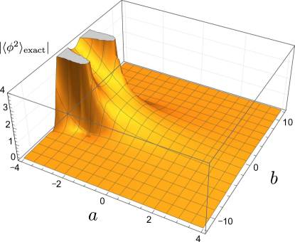
Figure 1: Absolute value of the exact answer of $\langle\phi^{2}\rangle_{\text{exact}}$ as a function of the real part $a$ and the imaginary part $b$ of the quadratic coefficient $\alpha$.

Figure 1 shows $|\langle\phi^{2}\rangle_{\text{exact}}|$ as a function of $a$ and $b$. It is clear to see that the expectation value increases in the region for $a<0$, which is reminiscent of the spontaneous symmetry breaking. Of course, the present model does not have infinite degrees of freedom and, strictly speaking, the spontaneous symmetry breaking is impossible, i.e. $\langle\phi\rangle_{\text{exact}}=0$ always holds for any $a$. Nevertheless, we can understand that a situation similar to the spontaneous symmetry breaking occurs in the following sense. The integration (7) is dominated around the minima (saddle-points) of $S$ as obtained from $dS/d\phi=0$. For the present theory there are three saddle-points,

$$\bar{\phi}_{0}=0\;,\qquad\bar{\phi}_{\pm}=\pm\sqrt{-\alpha/\beta}\;.$$ (10)

Clearly $S=S_{0}=0$ at $\phi=\bar{\phi}_{0}$ and $S=S_{\pm}=-\alpha^{2}/4$ at $\phi=\bar{\phi}_{\pm}$. Therefore, as long as $\mathrm{Re}\,S_{\pm}<\mathrm{Re}\,S_{0}$, the integration is dominated around $\bar{\phi}_{\pm}$ and $\langle\phi^{2}\rangle_{\text{exact}}$ should behave like $-\alpha/\beta$ in the first approximation. There is no phase transition in a strict sense, but we may well identify this situation physically as an analogue of the ordered state.

The qualitative behavior, however, changes drastically at $|b|\simeq|a|$ with $a<0$ and, so to speak, the broken symmetry is restored in the region for $|b|>|a|$. The reason for this change is easy to understand from the above consideration. For $|b|>|a|$ we explicitly see $\mathrm{Re}\,S_{\pm}=-a^{2}+b^{2}>\mathrm{Re}\,S_{0}=0$, and so the integration is again dominated around $\bar{\phi}_{0}$ and the non-zero expectation values at $\bar{\phi}_{\pm}$ become irrelevant in effect. Thus, we may say that the ordered state is hindered by attenuation effects caused by large $b$.

In summary this theory has three characteristic and qualitatively distinct states depending on $a$ and $b$ as follows:

$a>0$ :		Normal State
$a<0,\;\;a^{2}\gtrsim b^{2}$ :		Ordered State
$a<0,\;\;b^{2}\gtrsim a^{2}$ :		Attenuated State

It is known that the CLE fails in the attenuated state for $a<0$ and $b^{2}\gtrsim a^{2}$, which we will closely investigate analytically using the Gaussian Ansatz. Also, it would be worth while mentioning that the convergence of the CLE simulation to the exact answer is proven in the region with $a>0$ and $b^{2}<3a^{2}$, while the CLE simulation may not work for higher order expectation values, $\langle\phi^{n}\rangle$ $(n\geq 4)$, in the region with $a>0$ and $b^{2}>3a^{2}$ even in the normal state Aarts:2013uza . For the moment we will focus on $\langle\phi^{2}\rangle$ and will test our method for $\langle\phi^{4}\rangle$ later.

III.2 Results from the CLE

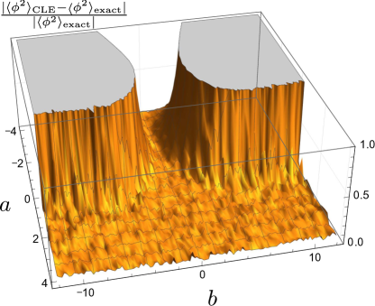
Figure 2: Comparison between the CLE results and the exact answer.

Here, we briefly discuss the results from the CLE to show where the CLE fails (for the two-point function). We numerically solved Eq. (1) for the action (7) with discretization $dt=5\times 10^{-3}$ and updated the fictitious time evolution by $10^{5}$ steps and average the numerical outputs over time. When we detected a runaway trajectory, we took $10^{3}$ steps back to avoid divergence.

We show the difference between the CLE results and the exact answer in Fig. 2. From this comparison we see that the CLE works good for $a>0$ generally (there may be a failure for the higher order functions Aarts:2013uza and we will come to this point in the end of this paper), and also it works in the ordered state with $a<0$ as long as $a^{2}>b^{2}$. We just note that in this theory the Stokes phenomenon occurs at $a=0$, and so the onset of the Stokes phenomenon does not necessarily coincide with the breakdown of the CLE simulation. As we mentioned before, the most problematic region for the CLE calculation in this theory is $a<0$ and $b^{2}\gtrsim a^{2}$, which we call the attenuated state throughout this present work.

IV Analysis with the Gaussian Ansatz

Because the Gaussian Ansatz is not an exact solution of the Fokker-Planck equation (2) for $\beta\neq 0$ in general, there is some ambiguity in the determination of $A$ and $B$ associated with the choice of what we optimize. A prescription we adopt here is an equilibrium condition for a two-point function, that is,

$$\int d\phi_{R}\,d\phi_{I}\,\phi^{2}\,\frac{dP[\phi]}{d\tau}=0\;,$$ (11)

which naturally must hold when $dP[\phi]/d\tau=0$ is reached. From the real and the imaginary parts of the above condition, we can get two equations to solve $A$ and $B$ as functions of $a$ and $b$. It should be noted that this condition has similarity to the “criteria for correctness” of the second order as discussed in Ref. Aarts:2013uza . Thus our condition naturally leads to a sort of gap equation in a sense that the $n$-th order “criteria for correctness” is equivalent to the Schwinger-Dyson equation of $n$-point function.

IV.1 Normal State

Plugging the action (7) into the Fokker-Planck equation (2), we can express $dP/d\tau$ and substitute it for Eq. (11). We can explicitly perform the Gaussian integrations with respect to $\phi_{R}$ and $\phi_{I}$ and after simplifying terms, we can find a set of equations to fix $A(\alpha,\beta)$ and $B(\alpha,\beta)$ as

$$A-a =\frac{3}{A^{2}+B^{2}}(cA+dB)\;,$$ (12)

$$B-b =\frac{3}{A^{2}+B^{2}}(dA-cB)\;.$$ (13)

It is easy to confirm that the non-interacting limit at $\beta=0$ (i.e. $c=d=0$) immediately leads to $A(\alpha,0)=a$ and $B(\alpha,0)=b$ as it should (and this free solution is nothing but the lowest order solution discussed in Ref. Aarts:2013uza ).

There are four independent branches of solutions for Eq. (13). For our present choice of $\beta=1$ (i.e. $c=1$ and $d=0$) the above set of equations leads to two complex and two real solutions. The real solution with $A>0$, which is required for the stability of the Gaussian integration, is uniquely determined as

$$A =\frac{a}{2}+\frac{1}{2\sqrt{2}}\sqrt{\!\sqrt{48a^{2}+(a^{2}\!+\!b^{2}\!-\!12)^{2}}+a^{2}\!-\!b^{2}\!+\!12}\;,$$ (14)

$$B =\frac{b}{2}+\frac{\text{sgn}(ab)}{2\sqrt{2}}\sqrt{\!\sqrt{48a^{2}+(a^{2}\!+\!b^{2}\!-\!12)^{2}}-a^{2}\!+\!b^{2}\!-\!12}\;.$$ (15)

It is clear that we can give an estimate for the two-point function using the Gaussian Ansatz in the following way,

$$\langle\phi^{2}\rangle_{\text{Gauss}}=\frac{\int d\phi_{R}\,d\phi_{I}\,\phi^{2}P[\phi]}{\int d\phi_{R}\,d\phi_{I}\,P[\phi]}=\frac{1}{A(\alpha,\beta)+iB(\alpha,\beta)}\;.$$ (16)

This final result from the Gaussian Ansatz is so simple in the analytical structure as compared to the exact answer, but we can confirm that this gives a good approximation in the normal state.

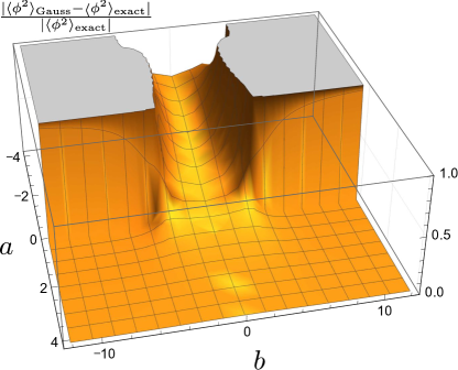
Figure 3: Comparison between the Gaussian Ansatz results and the exact answer for the quadratic operator.

To quantify how good the Gaussian Ansatz is, let us make a plot in a way similar to Fig. 2, with $\langle\phi^{2}\rangle_{\text{CLE}}$ replaced with $\langle\phi^{2}\rangle_{\text{Gauss}}$, which is presented in Fig. 3. It is very interesting to see that Fig. 3 has a remarkable similarity to Fig. 2. In particular the Gaussian Ansatz works excellently to show good agreement with the exact answer in the region with $a\geq 0$ for any $b$.

Our Gaussian Ansatz takes care of fluctuations around $\phi=\bar{\phi}_{0}$ and implicitly neglects the contributions from other saddle-points at $\phi=\bar{\phi}_{\pm}$. In terms of the Lefschetz thimble method, such an approximated treatment is justified by the fact that only the thimble attached to $\bar{\phi}_{0}$ makes a finite contribution for $a>0$. There is, however, a sudden change in the thimble structure at $a=0$, which is commonly called the Stokes phenomenon, and eventually all three thimbles attached to $\bar{\phi}_{0}$ and $\bar{\phi}_{\pm}$ come to make a finite contribution for $a<0$. This sudden change partially explains the sudden breakdown of the Gaussian Ansatz estimate around $a=0$.

One might have an impression that the Gaussian Ansatz may still work in the ordered state in view of Fig. 3 but some cautions are needed. In the region with $a^{2}>b^{2}$ and $a<0$, as $|a|$ grows up (and so the “condensate” grows up), the agreement gets worse. For example, at $a=-4$ and $b=0$ as shown in Fig. 3, $|\langle\phi^{2}\rangle_{\text{Gauss}}-\langle\phi^{2}\rangle_{\text{exact}}|/|\langle\phi^{2}\rangle_{\text{exact}}|\approx 0.5$ and the deviations would be larger with increasing $|a|$ in the negative direction. However, as we see from Fig. 2, the CLE should describe the physics correctly also in this region of the ordered state.

IV.2 Ordered State

In many physical examples the Stokes phenomenon makes the difficulty even more difficult. However, the CLE is capable of going beyond the Stokes phenomenon from the normal state to the ordered state except for the onset region. Although the most interesting question is what should be happening in the attenuated state as we will address later, let us clarify how the Gaussian Ansatz can capture the correct physics in the ordered state too.

In this region the contributions around $\bar{\phi}_{\pm}$ should be dominant, and so the Gaussian Ansatz must be formulated also around $\bar{\phi}_{\pm}$. In the mean-field type calculations it is a common technique to consider fluctuations around a shifted vacuum that is self-consistently determined by the energy minimization condition. Therefore, the probability weight should be changed as $P[\phi]\to P_{\pm}[\phi]=P[\phi+\bar{\phi}_{\pm}]$ with $A_{\pm}$ and $B_{\pm}$. Then, the two-point function should be approximated as

$$\langle\phi^{2}\rangle_{\text{Gauss}}=\frac{1}{A_{\pm}+iB_{\pm}}-\frac{\alpha}{\beta}\;,$$ (17)

where the last term represents the contribution by $\bar{\phi}_{\pm}^{2}=-\alpha/\beta$. The set of equations to fix $A_{\pm}$ and $B_{\pm}$ is slightly changed from Eq. (13) by $\bar{\phi}_{\pm}^{2}$ as

$$A_{\pm}+2a =\frac{3}{A_{\pm}^{2}+B_{\pm}^{2}}(cA_{\pm}+dB_{\pm})\;,$$ (18)

$$B_{\pm}+2b =\frac{3}{A_{\pm}^{2}+B_{\pm}^{2}}(dA_{\pm}-cB_{\pm})\;.$$ (19)

We can solve the above easily to find the analytical expressions again.

Here, let us make a remark on the convergence to the right solution. Generally speaking, beyond the Stokes phenomenon, multiple saddle-points take part in the integration; all of $\bar{\phi}_{0}$ and $\bar{\phi}_{\pm}$ in the present case. In physical applications it is often the case that one of them dominates the physics. The spontaneous symmetry breaking is such a phenomenon that can be correctly described by one saddle-point property. Because our 1-dimensional theory does not have such symmetry breaking, we have to sum up both contributions from $\bar{\phi}_{\pm}$ to have $\langle\phi\rangle=0$, but with infinite degrees of freedom only one contribution is spontaneously chosen, and thus the CLE method should work better then. Some other special examples are known to be more problematic. The mixed phase associated with a first-order phase transition should be one of the most typical examples. In such a situation contributions from different saddle-points are equally important, and also missing of a relative complex phase may cause a further problem of falling into a wrong answer Hayata:2015lzj . Another famous example is the Silver Blaze problem for which relative phases from infinite saddle-points make destructive interference Tanizaki:2015rda . For these problems, to formulate the Gaussian Ansatz to work, we need to take a proper superposition of $P_{0}[\phi]$ centered at $\bar{\phi}_{0}$ and $P_{\pm}[\phi]$ centered at $\bar{\phi}_{\pm}$ with relative weights including complex phase factors.

IV.3 Attenuated State

The most interesting and non-trivial question is why the CLE simulation and also the Gaussian Ansatz do not work in the attenuated state with $a<0$ and $b^{2}\gtrsim a^{2}$. This is beyond the Stokes phenomenon, but because of the real weight, $e^{-\mathrm{Re}\,S}=e^{-(b^{2}-a^{2})/4}\ll 1$, we can safely neglect these contributions from $\bar{\phi}_{\pm}$ for $b^{2}\gg a^{2}$ and the integration should be well approximated by the fluctuations around $\bar{\phi}_{0}$ only. Thus, it is very likely that the CLE simulation and the Gaussian Ansatz should be valid descriptions, but they fail in practice. Because the Gaussian Ansatz enables us to cope with the problem with simple analytical formulas, we can relatively easily identify the source of the problem.

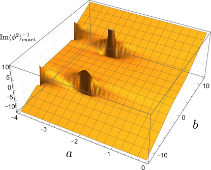
Figure 4: Counter part of $B$ inferred from $\langle\phi^{2}\rangle_{\text{exact}}$ as a function of $a$ and $b$ in the region for $a<0$.

It is already apparent from Eq. (15) how the Gaussian Ansatz leads to unphysical behavior. Let us consider expected behavior of $B$ for asymptotically large $b$. Naturally, we would immediately anticipate $B\simeq b$ for large enough $b$ from our physical intuition, and Eq. (15) indeed predicts $B\to b$ for $|b|\gg a$ as long as $a>0$, while it gives $B\to 0$ for $|b|\gg|a|$ once the system enters $a<0$. This is a very clear manifestation of where the wrong answer is picked up. Actually, the exact answer certainly exhibits the behavior of $B\simeq b$ even in the $a<0$ region, as checked in Fig. 4 where a counter part of $B$ defined by $\mathrm{Im}\,\langle\phi^{2}\rangle_{\text{exact}}^{-1}$ is plotted as a function of $a$ and $b$. Apart from the ordered state for $a<0$, $a^{2}>b^{2}$ and some spiky structures near the phase border, $\mathrm{Im}\,\langle\phi^{2}\rangle_{\text{exact}}^{-1}$ clearly scales as $\sim b$ in a way consistent with our intuition.

We already pointed out that there is another real solution of the set of equations (13), whose explicit forms are

$$\tilde{A} =\frac{a}{2}-\frac{1}{2\sqrt{2}}\sqrt{\!\sqrt{48a^{2}+(a^{2}\!+\!b^{2}\!-\!12)^{2}}+a^{2}\!-\!b^{2}\!+\!12}\;,$$ (20)

$$\tilde{B} =\frac{b}{2}-\frac{\text{sgn}(ab)}{2\sqrt{2}}\sqrt{\!\sqrt{48a^{2}+(a^{2}\!+\!b^{2}\!-\!12)^{2}}-a^{2}\!+\!b^{2}\!-\!12}\;.$$ (21)

The problem of this solution is that the integration with the Gaussian probability is not well-defined due to $\tilde{A}<0$ and we should usually exclude this branch of the solution.

Figure 5: Comparison in the $a<0$ region between the Gaussian Ansatz results with the unstable branch of solution and the exact answer.

For the moment let us postpone discussions on the stability but simply adopt the above branch of solution to evaluate new $\langle\tilde{\phi}^{2}\rangle_{\text{Gauss}}=1/(\tilde{A}+i\tilde{B})$ in the $a<0$ region. We show the comparison between $\langle\tilde{\phi}^{2}\rangle_{\text{Gauss}}$ and the exact answer in Fig. 5 and it is clear from this comparison that this new $\langle\tilde{\phi}^{2}\rangle_{\text{Gauss}}$ gives a very good approximation in the region with $a<0$ and $b^{2}>a^{2}$ (if sufficiently away from the phase boundary; see also the structure in Fig. 4). The important observation is that we take the difference between $\langle\tilde{\phi}^{2}\rangle_{\text{Gauss}}$ and $\langle\phi^{2}\rangle_{\text{exact}}$ before computing its absolute value, and so the good agreement seen in Fig. 5 includes the information on the complex phase. This means that, even though $\tilde{A}<0$ seems to be not allowed for convergence of the Gaussian integral, the exact answer indicates that this seemingly unstable $\tilde{A}<0$ is actually the right physical branch of solution.

Then, two questions arise. One is how such an unstable branch of solution can be the physical choice. Another one is what principle determines which branch of solution describes physically the correct behavior of the theory. These questions cannot be answered within the framework of the CLE or the Gaussian Ansatz of the CLE but we need more inputs from different approaches. Here, let us consider these questions by means of the Lefschetz thimble method. Figure 6 is a typical example of the thimble structures in the attenuated state for $a<0$ and $b^{2}\gg a^{2}$, and to draw Fig. 6 we chose $a=-0.1$ and $b=10$. From this we understand that the integration path along the thimble or the steepest descendent path is tilted from the real axis by $-\pi/4$ around $\bar{\phi}_{0}=0$ if $a<0$ and $b^{2}\gg a^{2}$.

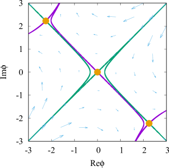
Figure 6: Steepest descendent paths (Lefschetz thimbles) shown by purple lines and steepest ascendent paths shown by green lines around three saddle-points shown by orange dots. Parameters are chosen as $a=-0.1$ and $b=10$.

Because we already know that the integral is dominated by the contribution near $\bar{\phi}_{0}$ only, we shall change the integration variable along the integration path as

$$\phi\;\longrightarrow\;\phi^{\prime}=e^{i\pi/4}\phi\;.$$ (22)

Let us point out that such a U(1) rotation makes sense only in the complexified description and this kind of transformation may be linked to the gauge cooling in the gauge theory. Then, the action (7) near $\bar{\phi}_{0}$ is expressed as

$$S\simeq\frac{1}{2}(-i\alpha)\phi^{\prime 2}=\frac{1}{2}(b-ia)\phi^{\prime 2}\;,$$ (23)

which implies that the roles of $a$ and $b$ should be switched to each other along this path. Needless to say, such a variable change causes another convergence problem from the $\phi^{4}$ term in the definition of the theory, but we are focusing only on the local properties around $\bar{\phi}_{0}$. Such a treatment shall be self-consistently justified if the probability distribution is localized well around $\bar{\phi}_{0}$. Now, because of Eq. (23), the probability distribution in the Gaussian Ansatz should be parametrized by $B^{\prime}$ instead of $A$ and $-A^{\prime}$ instead of $B$. Equations (13) should be also replaced as

$$B^{\prime}-b =\frac{3}{A^{\prime 2}+B^{\prime 2}}\cdot(-B^{\prime})\;,$$ (24)

$$-A^{\prime}+a =\frac{3}{A^{\prime 2}+B^{\prime 2}}(-A^{\prime})\;,$$ (25)

where $c=-1$ (after the change of $\phi\to\phi^{\prime}$) and $d=0$ are plugged in. Then, the above equations are completely identical to the original equations (13) having the same solutions of Eqs. (14), (15), and Eqs. (20), (21). Even though the solutions are just the same, this argument tells us an important implication – for the integration with the Gaussian Ansatz to converge around $\bar{\phi}_{0}$, what we need is $B>0$ and the sign of $A$ does not matter! In this way, the first question is answered now. Both branches of $A$, $B$ and $\tilde{A}$, $\tilde{B}$ are possible; Eqs. (15) and (21) lead to $B>0$ and $\tilde{B}>0$ for $b>0$. We note that the thimble would be tilted in the opposite direction for $b<0$ and then the convergence would require $B<0$ and $\tilde{B}<0$ which are also satisfied in Eqs. (15) and (21).

The second question is a little more non-trivial; both solutions seem to be equally possible from the integration stability condition. Besides, in the $a>0$ region, we have chosen Eqs. (14) and (15) from the condition of $A>0$ in the previous discussion, but even in this $A>0$ case, once we consider the path deformation along the Lefschetz thimble, the convergence condition around $\bar{\phi}_{0}$ is only the realness of $A$ and $B$. Hence, regardless of the sign of $A$, both solutions, Eqs. (14), (15) and Eqs. (20), (21), are possible.

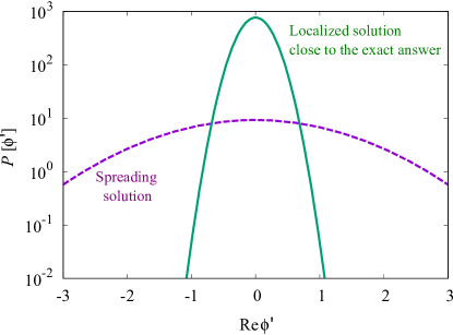
Figure 7: Gaussian profiles along the thimble near $\bar{\phi}_{0}$ corresponding to Eqs. (14), (15) (spreading solution by the dotted line) and Eqs. (20), (21) (localized solution by the solid line) for $a=-0.1$ and $b=10$.

For the self-consistent justification, the Gaussian width must be small. The Gaussian width along the thimble near $\bar{\phi}_{0}$ is determined by $\sqrt{A^{2}+B^{2}}$, and interestingly, we can readily find from Eqs. (14), (15), and Eqs. (20), (21) that

$$\begin{split}&\sqrt{A^{2}+B^{2}}\gg\sqrt{\tilde{A}^{2}+\tilde{B}^{2}}\quad\text{ for }\quad a>0\;,\\ &\sqrt{\tilde{A}^{2}+\tilde{B}^{2}}\gg\sqrt{A^{2}+B^{2}}\quad\text{ for }\quad a<0\;.\end{split}$$ (26)

This observation nicely explains which branch of solution should be picked up to describe the correct physics. For the demonstration purpose to visualize how the probability distributions spread, we plot $P[\phi^{\prime}]$ along the thimble in terms of $\phi^{\prime}$ in Fig. 7 and from this plot we see that the spreading distribution with Eqs. (14), (15) is not very well localized around $\bar{\phi}_{0}$ but it is stretched to the regions around $\bar{\phi}_{\pm}$, which already signals for falling into a wrong answer.

An interesting question is what then happens if we implement the CLE simulation after performing a rotation like Eq. (23) or more generally: $S[\phi^{\prime}]=\frac{1}{2}|\alpha|\phi^{\prime 2}+\frac{1}{4}\beta\,e^{-2i\theta}\phi^{\prime 4}$ where $\theta$ is an argument of a complex number $\alpha$ and $\phi^{\prime}=e^{i\theta/2}\phi$. Such a deformation of the theory might make the existence of the theory questionable, but we should remember that the existence of the theory is already subtle as soon as it is complexified because the complexified stochastic processes may always hit diverging rays on the complex plane; for the existence of the theory due to the cancellation of divergences, see discussions in Sec. 11.5 in Ref. Damgaard:1987rr . We may also say that we could have put a small $\phi^{\prime 4}$ term in the probability distribution that guarantees the convergence, which is dropped in the Gaussian Ansatz.

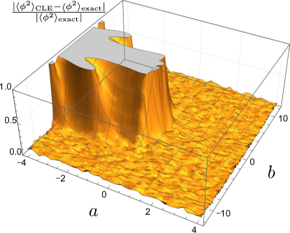
Figure 8: Comparison between the CLE results along the Lefschetz thimble and the exact answer for the quadratic operator.

Figure 8 shows our CLE results along the tilted path in terms of $\phi^{\prime}$. The structure for $a<0$ is surprisingly similar to the results in the Gaussian Ansatz with $\tilde{A}$ and $\tilde{B}$ presented in Fig. 5. This is a very clear numerical evidence about such a close relation between the CLE and the Gaussian Ansatz results. Summarizing our findings, the failure of the CLE simulation in the attenuated state as seen in Fig. 2 is attributed to the seemingly more stable but unphysically spreading solution, and if the CLE simulation is performed along the Lefschetz thimble without phase oscillation, the physical well-localized solution is correctly picked up to recover the exact answer. Again, we would emphasize that our proposed simple treatment of the Gaussian Ansatz is so powerful to explain all the good and bad behavior of the CLE simulations.

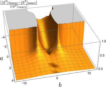
Figure 9: Comparison between the Gaussian Ansatz results and the exact answer for the quartic operator.

Another interesting and important question is whether the Gaussian Ansatz works for higher order operators or not. It has been argued in Ref. Aarts:2013uza that $\langle\phi^{4}\rangle$ cannot converge to the physical answer for $b^{2}>3a^{2}$ even in the $a>0$ region, while $\langle\phi^{2}\rangle$ can. Our optimistic guess is that the Gaussian Ansatz should be a valid description for higher order operators because the probability distribution is exponentially localized by construction. It is quite easy to check it by a generalization of Eq. (16), i.e.

$$\langle\phi^{4}\rangle_{\text{Gauss}}=\frac{3}{[A(\alpha,\beta)+iB(\alpha,\beta)]^{2}}\;.$$ (27)

Then, the comparison to the exact answer is shown in Fig. 9, which looks just like the comparison for $\langle\phi^{2}\rangle$ in Fig. 3. From this explicit comparison it is obvious that the Gaussian Ansatz definitely remains as a good approximation even for higher order operators in the region with $a>0$ and $b^{2}>3a^{2}$.

Now, a natural question is what happens in the numerical CLE simulation for $\langle\phi^{4}\rangle$. If the original action is put into the CLE simulation, we can indeed see sizable deviations of $\langle\phi^{4}\rangle_{\text{CLE}}$ from the exact answer even at $a>0$ in the $b^{2}\gg a^{2}$ region. If the simulation goes to higher and higher order operators, the failure region expands toward $b^{2}>3a^{2}$ gradually. Now, the most interesting question is whether the transformation from $\phi$ to $\phi^{\prime}$ can help the CLE simulation with approaching the exact answer. Figure 10 shows such a comparison. Surprisingly, it is evident that the convergence problem in the $a>0$ region has been completely resolved.

Figure 10: Comparison between the CLE results along the Lefschetz thimble and the exact answer for the quartic operator.

V Conclusion

We have exploited an approximation scheme using the Gaussian Ansatz to solve the Fokker-Planck equation and made quantitative comparisons between the complex Langevin equation, CLE, results and the Gaussian Ansatz results. Although the gap equations in the Gaussian Ansatz are so simple, we have confirmed that multiple solutions from them capture all the essential features of the CLE simulation not only for the successful regions but also for the unsuccessful regions.

Our most striking finding is that in the unsuccessful parameter regions one branch of solutions that is poorly localized is picked up by the Gaussian Ansatz and the CLE simulation, but another branch of solutions corresponds to the correct physical answer. To pick the correct one up, if the theory is reexpressed in terms of the variable along the Lefschetz thimble, the branch of solution that describes a more localized probability distribution can be picked up, which has been revealed by multiple solution structures in the Gaussian Ansatz. The idea has been tested in the CLE simulation also, and we have verified the consistency between the thimble-guided CLE simulation and the physical branch of solutions in the Gaussian Ansatz.

Our analysis implies a positive prospect in favor of the CLE simulation. Even when the convergence property is not sufficiently good leading to unphysical results, it does not necessarily mean the complete breakdown of the method itself. When it occurs, the CLE simulation may have multiple fixed points and it simply falls into where it should not fall into, though one of other fixed points may still correspond to the correct physics. This is very nice, because a minimal change in the treatment like the deformation of the integration path could help us with digging out the correct branch of solutions (see also the results in Refs. Aarts:2012ft ; Tsutsui:2015tua for other minimal changes to improve the correct convergence). This observation might have something to do with recently proposed ideas on the gauge cooling for the singular-drift problem Nagata:2015uga . It would be the most exciting challenge to apply our method of the Gaussian Ansatz to another theory like $S=-(\beta\cos\theta+i\theta)$ Ambjorn:1985iw which is the simplest integral that emulates the symmetry properties of lattice gauge theories.

- (1) E. Y. Loh, J. E. Gubernatis, R. T. Scalettar, S. R. White, D. J. Scalapino and R. L. Sugar, Phys. Rev. B41, 9301 (1990).
- (2) S. Muroya, A. Nakamura, C. Nonaka and T. Takaishi, Prog. Theor. Phys. 110, 615 (2003) [hep-lat/0306031].
- (3) S. Ejiri, PoS LATTICE 2008, 002 (2008) [arXiv:0812.1534 [hep-lat]].
- (4) K. Fukushima and T. Hatsuda, Rept. Prog. Phys. 74, 014001 (2011) [arXiv:1005.4814 [hep-ph]].
- (5) P. de Forcrand, PoS LAT 2009, 010 (2009) [arXiv:1005.0539 [hep-lat]].
- (6) G. Aarts, PoS LATTICE 2012, 017 (2012) [arXiv:1302.3028 [hep-lat]].
- (7) G. Aarts, J. Phys. Conf. Ser. 706, no. 2, 022004 (2016) [arXiv:1512.05145 [hep-lat]].
- (8) P. H. Damgaard and H. Huffel, Phys. Rept. 152, 227 (1987).
- (9) F. Karsch and H. W. Wyld, Phys. Rev. Lett. 55, 2242 (1985).
- (10) G. Aarts, L. Bongiovanni, E. Seiler, D. Sexty and I. O. Stamatescu, Eur. Phys. J. A 49, 89 (2013) [arXiv:1303.6425 [hep-lat]].
- (11) J. Berges and I.-O. Stamatescu, Phys. Rev. Lett. 95, 202003 (2005) [hep-lat/0508030]; J. Berges, S. Borsanyi, D. Sexty and I.-O. Stamatescu, Phys. Rev. D 75, 045007 (2007) [hep-lat/0609058]; J. Berges and D. Sexty, Nucl. Phys. B 799, 306 (2008) [arXiv:0708.0779 [hep-lat]].
- (12) R. Anzaki, K. Fukushima, Y. Hidaka and T. Oka, Annals Phys. 353, 107 (2015) [arXiv:1405.3154 [hep-ph]].
- (13) K. Fukushima and T. Hayata, Phys. Lett. B 735, 371 (2014) [arXiv:1403.4177 [hep-th]].
- (14) J. M. Pawlowski and C. Zielinski, Phys. Rev. D 87, no. 9, 094503 (2013) [arXiv:1302.1622 [hep-lat]]; Phys. Rev. D 87, no. 9, 094509 (2013) [arXiv:1302.2249 [hep-lat]].
- (15) K. Nagata, J. Nishimura and S. Shimasaki, PTEP 2016, no. 1, 013B01 (2016) [arXiv:1508.02377 [hep-lat]]; K. Nagata, J. Nishimura and S. Shimasaki, arXiv:1604.07717 [hep-lat]; arXiv:1606.07627 [hep-lat].
- (16) A. Mollgaard and K. Splittorff, Phys. Rev. D 88, no. 11, 116007 (2013) [arXiv:1309.4335 [hep-lat]]; Phys. Rev. D 91, no. 3, 036007 (2015) [arXiv:1412.2729 [hep-lat]].
- (17) G. Aarts and K. Splittorff, JHEP 1008, 017 (2010) [arXiv:1006.0332 [hep-lat]].
- (18) G. Aarts, F. A. James, J. M. Pawlowski, E. Seiler, D. Sexty and I. O. Stamatescu, JHEP 1303, 073 (2013) [arXiv:1212.5231 [hep-lat]].
- (19) G. Aarts, P. Giudice and E. Seiler, Annals Phys. 337, 238 (2013) [arXiv:1306.3075 [hep-lat]].
- (20) J. Nishimura and S. Shimasaki, Phys. Rev. D 92, no. 1, 011501 (2015) [arXiv:1504.08359 [hep-lat]].
- (21) T. Hayata, Y. Hidaka and Y. Tanizaki, arXiv:1511.02437 [hep-lat].
- (22) G. Aarts, Phys. Rev. Lett. 102, 131601 (2009) [arXiv:0810.2089 [hep-lat]].
- (23) G. Aarts, JHEP 0905, 052 (2009) [arXiv:0902.4686 [hep-lat]].
- (24) D. Sexty, Phys. Lett. B 729, 108 (2014) [arXiv:1307.7748 [hep-lat]].
- (25) G. Aarts, E. Seiler, D. Sexty and I. O. Stamatescu, Phys. Rev. D 90, no. 11, 114505 (2014) [arXiv:1408.3770 [hep-lat]].
- (26) Z. Fodor, S. D. Katz, D. Sexty and C. Torok, Phys. Rev. D 92, no. 9, 094516 (2015) [arXiv:1508.05260 [hep-lat]].
- (27) G. Aarts, F. Attanasio, B. Jaeger and D. Sexty, arXiv:1606.05561 [hep-lat].
- (28) E. Seiler, D. Sexty and I. O. Stamatescu, Phys. Lett. B 723, 213 (2013) [arXiv:1211.3709 [hep-lat]].
- (29) G. Aarts and I. O. Stamatescu, JHEP 0809, 018 (2008) [arXiv:0807.1597 [hep-lat]].
- (30) G. Aarts, E. Seiler and I. O. Stamatescu, Phys. Rev. D 81, 054508 (2010) doi:10.1103/PhysRevD.81.054508 [arXiv:0912.3360 [hep-lat]].
- (31) G. Aarts, Phys. Rev. D 88, no. 9, 094501 (2013) [arXiv:1308.4811 [hep-lat]].
- (32) G. Aarts, L. Bongiovanni, E. Seiler and D. Sexty, JHEP 1410, 159 (2014) [arXiv:1407.2090 [hep-lat]].
- (33) K. Fukushima and Y. Tanizaki, PTEP 2015, no. 11, 111A01 (2015) [arXiv:1507.07351 [hep-th]].
- (34) S. Tsutsui and T. M. Doi, arXiv:1508.04231 [hep-lat].
- (35) E. Witten, AMS/IP Stud. Adv. Math. 50, 347 (2011) [arXiv:1001.2933 [hep-th]]; arXiv:1009.6032 [hep-th].
- (36) M. Cristoforetti, L. Scorzato and F. Di Renzo, J. Phys. Conf. Ser. 432, 012025 (2013) [arXiv:1210.8026 [hep-lat]].
- (37) L. Scorzato, arXiv:1512.08039 [hep-lat].
- (38) H. Fujii, D. Honda, M. Kato, Y. Kikukawa, S. Komatsu and T. Sano, JHEP 1310, 147 (2013) [arXiv:1309.4371 [hep-lat]].
- (39) M. Cristoforetti et al. [AuroraScience Collaboration], Phys. Rev. D 86, 074506 (2012) [arXiv:1205.3996 [hep-lat]].
- (40) Y. Tanizaki, Phys. Rev. D 91, no. 3, 036002 (2015) [arXiv:1412.1891 [hep-th]].
- (41) H. Fujii, S. Kamata and Y. Kikukawa, JHEP 1511, 078 (2015) Erratum: [JHEP 1602, 036 (2016)] [arXiv:1509.08176 [hep-lat]]; JHEP 1512, 125 (2015) [arXiv:1509.09141 [hep-lat]].
- (42) A. Mukherjee and M. Cristoforetti, Phys. Rev. B 90, no. 3, 035134 (2014) [arXiv:1403.5680 [cond-mat.str-el]].
- (43) T. Kanazawa and Y. Tanizaki, JHEP 1503, 044 (2015) [arXiv:1412.2802 [hep-th]].
- (44) Y. Tanizaki, Y. Hidaka and T. Hayata, New J. Phys. 18, no. 3, 033002 (2016) [arXiv:1509.07146 [hep-th]].
- (45) T. D. Cohen, Phys. Rev. Lett. 91, 222001 (2003) [hep-ph/0307089].
- (46) K. Splittorff and J. J. M. Verbaarschot, Phys. Rev. Lett. 98, 031601 (2007) [hep-lat/0609076].
- (47) A. Behtash, T. Sulejmanpasic, T. Schaefer and M. Unsal, Phys. Rev. Lett. 115, no. 4, 041601 (2015) [arXiv:1502.06624 [hep-th]].
- (48) P. A. Amundsen and P. H. Damgaard, Phys. Rev. D 29, 323 (1984).
- (49) Y. Grandati, A. Berard and P. Grange, Phys. Lett. B 276, 141 (1992); Phys. Lett. B 304, 298 (1993).
- (50) J. Greensite, Phys. Rev. D 90, no. 11, 114507 (2014) [arXiv:1406.4558 [hep-lat]].
- (51) Y. Tanizaki, H. Nishimura and K. Kashiwa, Phys. Rev. D 91, no. 10, 101701 (2015) [arXiv:1504.02979 [hep-th]].
- (52) K. Fukushima and Y. Hidaka, Phys. Rev. D 75, 036002 (2007) [hep-ph/0610323].
- (53) J. R. Klauder and W. P. Petersen, J. Stat. Phys. 39, 53 (1985).
- (54) J. Ambjorn and S. K. Yang, Phys. Lett. B 165, 140 (1985).