Towards Analytics Aware Ontology Based Access
to Static and Streaming Data
(Extended Version)

Abstract

Real-time analytics that requires integration and aggregation of heterogeneous and distributed streaming and static data is a typical task in many industrial scenarios such as diagnostics of turbines in Siemens. OBDA approach has a great potential to facilitate such tasks; however, it has a number of limitations in dealing with analytics that restrict its use in important industrial applications. Based on our experience with Siemens, we argue that in order to overcome those limitations OBDA should be extended and become analytics, source, and cost aware. In this work we propose such an extension. In particular, we propose an ontology, mapping, and query language for OBDA, where aggregate and other analytical functions are first class citizens. Moreover, we develop query optimisation techniques that allow to efficiently process analytical tasks over static and streaming data. We implement our approach in a system and evaluate our system with Siemens turbine data.

1 Introduction

Ontology Based Data Access (OBDA) [1] is an approach to access information stored in multiple datasources via an abstraction layer that mediates between the datasources and data consumers. This layer uses an ontology to provide a uniform conceptual schema that describes the problem domain of the underlying data independently of how and where the data is stored, and declarative mappings to specify how the ontology is related to the data by relating elements of the ontology to queries over datasources. The ontology and mappings are used to transform queries over ontologies, i.e., ontological queries, into data queries over datasources. As well as abstracting away from details of data storage and access, the ontology and mappings provide a declarative, modular and query-independent specification of both the conceptual model and its relationship to the data sources; this simplifies development and maintenance and allows for easy integration with existing data management infrastructure.

A number of systems that at least partially implement OBDA have been recently developed; they include D2RQ [2], Mastro [3], morph-RDB [4], Ontop [5], OntoQF [6], Ultrawrap [7], Virtuoso, Spyder, and others [8, 9]. Some of them were successfully used in various applications including cultural heritage [10], governmental organisations [11], and industry [12, 13]. Despite their success, OBDA systems, however, are not tailored towards analytical tasks that are naturally based on data aggregation and correlation. Moreover, they offer a limited or no support for queries that combine streaming and static data. A typical scenario that requires both analytics and access to static and streaming data is diagnostics and monitoring of turbines in Siemens.

Siemens has several service centres dedicated to diagnostics of thousands of power-generation appliances located across the globe [13]. One typical task of such a centre is to detect in real-time potential faults of a turbine caused by, e.g., an undesirable pattern in temperature’s behaviour within various components of the turbine. Consider a (simplified) example of such a task:

In a given turbine report all temperature sensors that are reliable, i.e., with the average score of validation tests at least 90%, and whose measurements within the last 10 min were similar, i.e., Pearson correlated by at least 0.75, to measurements reported last year by a reference sensor that had been functioning in a critical mode.

This task requires to extract, aggregate, and correlate static data about the turbine’s structure, streaming data produced by up to 2,000 sensors installed in different parts of the turbine, and historical operational data of the reference sensor stored in multiple datasources. Accomplishing such a task currently requires to pose a collection of hundreds of queries, the majority of which are semantically the same (they ask about temperature), but syntactically differ (they are over different schemata). Formulating and executing so many queries and then assembling the computed answers take up to 80% of the overall diagnostic time that Siemens engineers typically have to spend [13]. The use of ODBA, however, would allow to save a lot of this time since ontologies can help to ‘hide’ the technical details of how the data is produced, represented, and stored in data sources, and to show only what this data is about. Thus, one would be able to formulate this diagnostic task using only one ontological query instead of a collection of hundreds data queries that today have to be written or configured by IT specialists. Clearly, this collection of queries does not disappear: the OBDA query tranformation will automatically compute them from the the high-level ontological query using the ontology and mappings.

Siemens analytical tasks as the one in the example scenario typically make heavy use of aggregation and correlation functions as well as arithmetic operations. In our running example, the aggregation function ${\sf{min}}$ and the comparison operator $\geq$ are used to specify what makes a sensor reliable and to define a threshold for similarity. Performing such operations only in ontological queries, or only in data queries specified in the mappings is not satisfactory. In the case of ontological queries, all relevant values should be retrieved prior to performing grouping and arithmetic operations. This can be highly inefficient, as it fails to exploit source capabilities (e.g., access to pre-computed averages), and value retrieval may be slow and/or costly, e.g., when relevant values are stored remotely. Moreover, it adds to the complexity of application queries, and thus limits the benefits of the abstraction layer. In the case of source queries, aggregation functions and comparison operators may be used in mapping queries. This is brittle and inflexible, as values such as 90% and 0.75, which are used to define ‘reliable sensor’ and ‘similarity’, cannot be specified in the ontological query, but must be ‘hard-wired’ in the mappings, unless an appropriate extension to the query language or the ontology are developed. In order to address these issues, OBDA should become

analytics-aware by supporting declarative representations of basic analytics operations and using these to efficiently answer higher level queries.

In practice this requires enhancing OBDA technology with ontologies, mappings, and query languages capable of capturing operations used in analytics, but also extensive modification of OBDA query preprocessing components, i.e., reasoning and query transformation, to support these enhanced languages.

Moreover, analytical tasks as in the example scenario should typically be executed continuously in data intensive and highly distributed environments of streaming and static data. Efficiency of such execution requires non-trivial query optimisation. However, optimisations in existing OBDA systems are usually limited to minimisation of the textual size of the generated queries, e.g. [14], with little support for distributed query processing, and no support for optimisation for continuous queries over sequences of numerical data and, in particular, computation of data correlation and aggregation across static and streaming data. In order to address these issues, OBDA should become

source and cost aware by supporting both static and streaming data sources and offering a robust query planning component and indexing that can estimate the cost of different plans, and use such estimates to produce low-cost plans.

Note that the existence of materialised and pre-computed subqueries relevant to analytics within sources and archived historical data that should be correlated with current streaming data implies that there is a range of query plans which can differ dramatically with respect to data transfer and query execution time.

In this paper we make the first step to extend OBDA systems towards becoming analytics, source, and cost aware and thus meeting Siemens requirements for turbine diagnostics tasks. In particular, our contributions are the following:

• We proposed analytics-aware OBDA components, i.e., (i) ontology language $\textit{DL-Lite}_{\cal A}^{\sf agg}$ that extends $\textit{DL-Lite}_{\cal A}$ with aggregate functions as first class citizens, (ii) query language STARQL over ontologies that combine streaming and static data, and (iii) a mapping language relating $\textit{DL-Lite}_{\cal A}^{\sf agg}$ vocabulary and STARQL constructs with relational queries over static and streaming data.

• We developed efficient query transformation techniques that allow to turn STARQL queries over $\textit{DL-Lite}_{\cal A}^{\sf agg}$ ontologies, into data queries using our mappings.

• We developed source and cost aware (i) optimisation techniques for processing complex analytics on both static and streaming data, including adaptive indexing schemes and pre-computation of frequent aggregates on user queries, and (ii) elastic infrastructure that automatically distributes analytical computations and data over a computational cloud for fastet query execution.

• We implemented (i) a highly optimised engine ExaStream capable of handling complex streaming and static queries in real time, (ii) a dedicated STARQL2SQL^⊕ translator that transforms STARQL queries into queries over static and streaming data, (iii) an integrated OBDA system that relies on our and third party components.

• We conducted a performance evaluation of our OBDA system with large scale Siemens simulated data using analytical tasks.

The paper is organised as follows: Sec. 2 presents our analytics-aware ontology, query, and mapping languages as well as query optimisation techniques; Sec. 3 and 4 discuss implementation of our system and presents experiments; Sec. 5 discusses related work.

2 Analytics Aware OBDA for Static and Streaming Data

In this section we first introduce our analytics-aware ontology language $\textit{DL-Lite}_{\cal A}^{\sf agg}$ (Sec. 2.1) for capturing static aspects of the domain of interest. In $\textit{DL-Lite}_{\cal A}^{\sf agg}$ ontologies, aggregate functions are treated as first class citizens. Then, in Sec 2.2 we will introduce a query language STARQL that allows to combine static conjunctive queries over $\textit{DL-Lite}_{\cal A}^{\sf agg}$ with continuous diagnostic queries that involve simple combinations of time aware data attributes, time windows, and functions, e.g., correlations over streams of attribute values. Using STARQL queries one can retrieve entities, e.g., sensors, that pass two ‘filters’: static and continuous. In our running example a static ‘filter’ checks whether a sensor is reliable, while a continuous ‘filter’ checks whether the measurements of the sensor are Pearson correlated with the measurements of reference sensor. In Sec. 2.3 we will explain how to translate STARQL queries into data queries by mapping $\textit{DL-Lite}_{\cal A}^{\sf agg}$ concepts, properties, and attributes occurring in queries to database schemata and by mapping functions and constructs of STARQL continuous ‘filters’ into corresponding functions and constructs over databases. Finally, in Sec. 2.4 we discuss how to optimise resulting data queries.

2.1 Ontology Language

Our ontology language, $\textit{DL-Lite}_{\cal A}^{\sf agg}$, is an extension of $\textit{DL-Lite}_{\cal A}$ [1] with concepts that are based on aggregation of attribute values. The semantics for such concepts adapts the closed-world semantics [15]. The main reason why we rely on this semantics is to avoid the problem of empty answers for aggregate queries under the certain answers semantics [16, 17]. In $\textit{DL-Lite}_{\cal A}^{\sf agg}$ we distinguish between individuals and data values from countable sets $\Delta$ and $D$ that intuitively correspond to the datatypes of RDF. We also distinguish between atomic roles $P$ that denote binary relations between pairs of individuals, and attributes $F$ that denote binary relations between individuals and data values. For simplicity of presentation we assume that $D$ is the set of rational numbers. Let ${\sf{agg}}$ be an aggregate function, e.g., ${\sf{min}}$, ${\sf{max}}$, ${\sf{count}}$, ${\sf{countd}}$, ${\sf{sum}}$, or ${\sf{avg}}$, and let $\circ$ be a comparison predicate on rational numbers, e.g., $\geq,\leq,<,>,=,$ or $\neq$.

2.1.1 $\textit{DL-Lite}_{\cal A}^{\sf agg}$ Syntax.

The grammar for concepts and roles in $\textit{DL-Lite}_{\cal A}^{\sf agg}$ is as follows:

$$B\rightarrow A\mid\exists R,\quad C\rightarrow B\mid\exists F,\quad E\rightarrow\circ_{r}({\sf{agg}}\ F),\quad R\rightarrow P\mid P^{-},$$

where $F$, $P$, ${\sf{agg}}$, and $\circ$ are as above, $r$ is a rational number, $A$, $B$, $C$ and $E$ are atomic, basic, extended and aggregate concepts, respectively, and $R$ is a basic role.

A $\textit{DL-Lite}_{\cal A}^{\sf agg}$ ontology $\mathcal{O}$ is a finite set of axioms. We consider two types of axioms: aggregate axioms of the form $E\sqsubseteq B$ and regular axioms that take one of the following forms: (i) inclusionsof the form $C\sqsubseteq B$, $R_{1}\sqsubseteq R_{2}$, and $F_{1}\sqsubseteq F_{2}$, (ii) functionalityaxioms $({\sf funct}\ R)$ and $({\sf funct}\ F),$ (iii) or denials of the form $B_{1}\sqcap B_{2}\sqsubseteq\bot$, $R_{1}\sqcap R_{2}\sqsubseteq\bot$, and $F_{1}\sqcap F_{2}\sqsubseteq\bot$. As in $\textit{DL-Lite}_{\cal A}$, a $\textit{DL-Lite}_{\cal A}^{\sf agg}$ dataset $\mathcal{D}$ is a finite set of assertions of the form: $A(a)$, $R(a,b)$, and $F(a,v)$.

We require that if $({\sf funct}\ R)$ (resp., $({\sf funct}\ F)$) is in $\mathcal{O}$, then $R^{\prime}\sqsubseteq R$ (resp., $F^{\prime}\sqsubseteq F$) is not in $\mathcal{O}$ for any $R^{\prime}$ (resp., $F^{\prime}$). This syntactic condition, as wel as the fact that we do not allow concepts of the form $\exists F$ and aggregate concepts to appear on the right-hand side of inclusions ensure good computational properties of $\textit{DL-Lite}_{\cal A}^{\sf agg}$. The former is inherited from $\textit{DL-Lite}_{\cal A}$, while the latter can be shown using techniques of [15].

Consider the ontology capturing the reliability of sensors as in our running example:

$$\mathit{precisionScore}\sqsubseteq\mathit{testScore},\quad\geq_{0.9}({\sf{min}}\ \mathit{testScore})\sqsubseteq\sf\mathit{Reliable},$$ (1)

where $\mathit{Reliable}$ is a concept, $precisionScore$ and $\mathit{testScore}$ are attributes, and finally $\geq_{0.9}\sf(min\ \mathit{testScore})$ is an aggregate concept that captures individuals with one or more $\mathit{testScore}$ values whose minimum is at least $0.9$.

2.1.2 $\textit{DL-Lite}_{\cal A}^{\sf agg}$ Semantics.

We define the semantics of $\textit{DL-Lite}_{\cal A}^{\sf agg}$ in terms of first-order interpretations over the union of the countable domains $\Delta$ and $D$. We assume the unique name assumption and that constants are interpreted as themselves, i.e., $a^{\mathcal{I}}=a$ for each constant $a$; moreover, interpretations of regular concepts, roles, and attributes are defined as usual (see [1] for details) and for aggregate concepts as follows:

$$(\circ_{r}({\sf{agg}}\ F))^{\mathcal{I}}=\{a\in\Delta\mid{\sf{agg}}\{|v\in D\mid(a,v)\in F^{\mathcal{I}}|\}\circ r\}.$$

Here $\{|\cdot|\}$ denotes a multi-set. Similarly to [15], we say that an interpretation $\mathcal{I}$ is a model of $\mathcal{O}\cup\mathcal{D}$ if two conditions hold: (i) $\mathcal{I}\models\mathcal{O}\cup\mathcal{D}$, i.e., $\mathcal{I}$ is a first-order model of $\mathcal{O}\cup\mathcal{D}$ and (ii) $F^{\mathcal{I}}=\{(a,v)\mid F(a,v)\text{ is in the deductive closure of }\mathcal{D}\text{ with }\mathcal{O}\}$for each attribute $F$. Here, by deductive closure of $\mathcal{D}$ with $\mathcal{O}$ we assume a dataset that can be obtained from $\mathcal{D}$ using the chasing procedure with $\mathcal{O}$, as described in [1]. One can show that for $\textit{DL-Lite}_{\cal A}^{\sf agg}$ satisfiability of $\mathcal{O}\cup\mathcal{D}$ can be checked in time polynomial in $|\mathcal{O}\cup\mathcal{D}|$.

As an example consider a dataset consisting of assertions: $\mathit{precisionScore}(s_{1},0.9)$, $\mathit{testScore}(s_{2},0.95)$, and $\mathit{testScore}(s_{3},0.5)$. Then, for every model $\mathcal{I}$ of these assertions and the axioms in Eq. (1), it holds that $(\geq_{0.9}({\sf{min}}\ \mathit{precisionScore}))^{\mathcal{I}}=\{s_{1}\}$, $(\geq_{0.9}({\sf{min}}\ \mathit{testScore}))^{\mathcal{I}}=\{s_{1},s_{2}\}$, and thus $\{s_{1},s_{2}\}\subseteq\mathit{Reliable}^{\mathcal{I}}$.

2.1.3 Query Answering.

Let $\mathcal{Q}$ be the class of conjunctive queries over concepts, roles, and attributes, i.e., each query $q\in\mathcal{Q}$ is an expression of the form: $q(\vec{x})\text{ :- }{\sf conj}(\vec{x}),$ where $q$ is of arity $k$, ${\sf conj}$ is a conjunction of atoms $A(u)$, $E(v)$, $R(w,z)$, or $F(w,z)$, and $u$, $v$, $w$, $z$ are from $\vec{x}$. Following the standard approach for ontologies, we adapt certain answers semantics for query answering:

$${\sf cert}(q,\mathcal{O},\mathcal{D})=\{\vec{t}\in(\Delta\cup D)^{k}\mid\mathcal{I}\models{\sf conj}(\vec{t})\text{ for each model }\mathcal{I}\text{ of }\mathcal{O}\cup\mathcal{D}\}.$$

Continuing with our example, consider the query: $q(x)\text{ :- }\mathit{Reliable}(x)$ that asks for reliable sensors. The set of certain answers ${\sf cert}(q,\mathcal{O},\mathcal{D})$ for this $q$ over the example ontology and dataset is $\{s_{1},s_{2}\}$.

By relying on Theorem 1 of [15] and the fact that each aggregate concept behaves like a DL-Lite closed predicate of [15], in the sense that its interpretation—given an ontology $\mathcal{O}$ and dataset $\mathcal{D}$—is determined and fixed by $\mathcal{D}$, one can show that conjunctive query answering in $\textit{DL-Lite}_{\cal A}^{\sf agg}$ is tractable, assuming that computation of aggregate functions can be done in time polynomial in the size of the data. This can be shown by reducing conjunctive query answering over ontologies with aggregates to the one over aggregate free ontologies of [15]. Indeed, consider a DL-Lite ontology $\mathcal{O}^{\prime}$ and dataset $\mathcal{D}^{\prime}$ constructed as follows: $\mathcal{O}^{\prime}$ is obtained from $\mathcal{O}$ by replacing all aggregate concepts of the form $\circ_{r}({\sf{agg}}\ F)$ with a fresh closed predicate $U$ in every $\mathcal{O}$’s axiom containing $\circ_{r}({\sf{agg}}\ F)$; $\mathcal{D}^{\prime}$ extends $\mathcal{D}$ with the set of assertions $\{F(a,v)\mid F^{\prime}(a,v)\in\mathcal{D}\text{ and }\mathcal{O}\models F^{\prime}\sqsubseteq F\}$ and, $\{U(a)\mid{\sf{agg}}\{|d\mid F(a,v)\in\mathcal{D}^{\prime}|\}\circ r\}$. Observe that $\mathcal{O}^{\prime}$ is safe according to [15] and, hence, conjunctive query answering is tractable. Now, let $Q$ be a conjunctive query over $\mathcal{O}\cup\mathcal{D}$. Then, one can easily show that evaluation of a conjunctive query $Q$ over $\mathcal{O}\cup\mathcal{D}$ gives the same result as evaluation of $Q^{\prime}$, where each atom of the form $(\circ_{r}({\sf{agg}}\ F))(x)$ is replaced with $U(x)$, over $\mathcal{O}^{\prime}\cup\mathcal{D}^{\prime}$. Moreover, one can show that the standard query rewriting algorithm of [1] proposed for $\textit{DL-Lite}_{\cal A}$ as a part of query transformation procedure (with an extension discussed in Section 2.3) also works for $\textit{DL-Lite}_{\cal A}^{\sf agg}$ and SQL.

2.1.4 Discussion.

Note that our aggregate concepts can be encoded as aggregate queries over attributes as soon as the latter are interpreted under the closed-world semantics. Indeed, given $E=\circ_{r}({\sf{agg}}\ F)$, certain answers for the atomic query $q(x)\text{ :- }E(x)$ over this aggregate concept would be the same as for the following aggregate query over $F$:

$$Q_{E}(x)={\sf SELECT}\ \ x\ \ {\sf FROM}\ \ F(x,y)\ \ {\sf GROUP\ BY}\ \ x\ \ {\sf HAVING}\ \ {\sf{agg}}(y)\circ r.$$

Thus, one can reduce conjunctive query answering over our analytics aware $\textit{DL-Lite}_{\cal A}^{\sf agg}$ ontologies to aggregate query answering over classical $\textit{DL-Lite}_{\cal A}$ ontologies as soon as the closed-world semantics is exploited for the interpretation of data attributes. At the same time, we argue that in a number of applications, such as monitoring and diagnostics at Siemens [13], explicit aggregate concepts of $\textit{DL-Lite}_{\cal A}^{\sf agg}$ give us significant modelling and query formulation advantages over $\textit{DL-Lite}_{\cal A}$ since in such applications concepts are naturally based on aggregate values of potentially many different attributes. For instance, in Siemens the notion of reliability is naturally based on aggregation over various attributes, i.e., it should be modelled as $E_{i}\sqsubseteq\mathit{Reliable}$ for many dfferent aggregate concepts $E_{i}$, and reliability is also commonly exploited in diagnostic queries. In the case of $\textit{DL-Lite}_{\cal A}^{\sf agg}$, in all such diagnostic queries it suffices to use only one atom $\mathit{Reliable}(x)$. In contrast, in the case of $\textit{DL-Lite}_{\cal A}$, each such diagnostic query would have to contain the whole union $\mathit{Reliable}(x)\cup_{i}Q_{E_{i}}(x)$. (Alternatively, aggregation can be encoded in mappings as discussed in Section 2.3 and possibly adresseds with the help of materialised views which is a part of our future work—see the end of Section 6.) Thus, Siemens diagnostics queries over $\textit{DL-Lite}_{\cal A}$ would be much more complex than the ones over $\textit{DL-Lite}_{\cal A}^{\sf agg}$. Moreover, in the case of $\textit{DL-Lite}_{\cal A}$, $Q_{E_{i}}(x)$s in such diagnostics queries will have to be adjusted each time the notion of reliability is modified, while, in the case of $\textit{DL-Lite}_{\cal A}^{\sf agg}$, only the ontology and not the queries should be adjusted.

2.2 Query Language

STARQL is a query language over ontologies that allows to query both streaming and static data and supports not only standard aggregates such as count, avg, etc but also more advanced aggregation functions from our backend system such as Pearson correlation. In this section we will give an overview of the main language constructs and semantics of STARQL, and illustrate it on our running example (see [18] for more details on its semantics).

Each STARQL query takes as input a static $\textit{DL-Lite}_{\cal A}^{\sf agg}$ ontology and dataset as well as a set of live and historic streams. The output of the query is a stream of timestamped data assertions about objects that occur in the static input data and satisfy two kinds of filters: (i) a conjunctive query over the input static ontology and data and (ii) a diagnostic query over the input streaming data—which can be live and archived (i.e., static)— that may involve typical mathematical, statistical, and event pattern features needed in real-time diagnostic scenarios. The syntax of STARQL is inspired by the W3C standardised SPARQL query language; it also allows for nesting of queries. Moreover, STARQL has a formal semantics that combines open and closed-world reasoning and extends snapshot semantics for window operators [19] with sequencing semantics that can handle integrity constraints such as functionality assertions.

In Fig. 1 we present a STARQL query that captures the diagnostic task from our running example and uses concepts, roles, and attributes from our Siemens ontology [13, 20, 21, 22, 23, 24, 25] and Eq. (1). The query has three parts: declaration of the output stream (Lines 5 and 6), sub-query over the static data (Lines 8 and 9) that in the running example corresponds to ‘return all temperature sensors that are reliable, i.e., with the average score of validation tests at least 90%’ and sub-query over the streaming data (Lines 11–17) that in the running example corresponds to ‘whose measurements within the last 10 min Pearson correlate by at least 0.75 to measurements reported by a reference sensor last year’. Moreover, in Line 1 there is declarations of the namespace that is used in the sub-queries, i.e., the URI of the Siemens ontology, and in Line 3 there is a declaration of the pulse of the streaming sub-query. We now enumerate the main clauses of STARQL and illustrate them using the query in Fig. 1:

keywordstyle=, basicstyle=, language=sql, morekeywords=CREATE, STREAM, CONSTRUCT, GRAPH, NOW, SEQUENCE, STATIC, ABOX, TBOX, ONTOLOGY, DATA, EXISTS, FORALL, MAX, AGGREGATE, IF, THEN, STREAM, PULSE, PREFIX, WITH, START, FREQUENCY, sec, numbers=left, numberstyle=, numbersep=4pt, breaklines=true, frame=lines, rulecolor=, framerule=0.5pt, backgroundcolor=, aboveskip=1em, belowskip=1em, showstringspaces=false, tabsize=3, framesep=1em

⬇

PREFIX ex : <http://www.siemens.com/onto/gasturbine/>

CREATE PULSE examplePulse WITH START = NOW, FREQUENCY = 1min

CREATE STREAM StreamOfSensorsInCriticalMode AS

CONSTRUCT GRAPH NOW { ?sensor a :InCriticalMode }

FROM STATIC ONTOLOGY ex:sensorOntology, DATA ex:sensorStaticData

WHERE { ?sensor a ex:Reliable }

FROM STREAM sensorMeasurements [NOW - 1min, NOW]-> 1sec

referenceSensorMeasurements 1year <-[NOW - 1min, NOW]-> 1sec,

USING PULSE examplePulse

SEQUENCE BY StandardSequencing AS MergedSequenceOfMeasurementes

HAVING EXISTS i IN MergedSequenceOfMeasurementes

(GRAPH i { ?sensor ex:hasValue ?y. ex:refSensor ex:hasValue ?z })

HAVING PearsonCorrelation(?y, ?z) > 0.75

Figure 1: Running example query expressed in STARQL

1. clause declares the name of the output stream. In our example the output stream is called StreamOfSensorsInCriticalMode.

2. clause defines how the output stream declared in the previous clause should be formed. STARQL allows for two types of output: the SELECT clause forms the output as simply the lists of variable bindings, and the CONSTRUCT clause defines the output as an RDF graph that further can be stored in an RDF datastore or sent as input to another STARQL query. In our example, we form the output as a set of data assertion of the form $A(b)$, thus making an RDF graph consisting of all sensors (i.e., ?sensor) that function in a critical mode (i.e, ex:InCriticalMode) and are determined by the two sub-queries.

3. clause declares input static ontology and data and defines streaming data with window parameters using the start and end value, e.g., ‘[NOW - 1min, NOW]’, as well as a slide parameter, e.g., ‘-> 1sec’. In our example, we have the static ontology ex:sensorOntology and data DATA ex:sensorStaticData and two streams: sensorMeasurements of live sensor measurements and also referenceSensorMeasurements of recorded measurements of the reference sensor. Note that the recorded sensor uses a set back time of one year, that is, values from one year ago are correlated to a live stream.

4. clause defines the periodic pulse for the input streams, given by an execution frequency, e.g., 1min and its absolute start and/or end time, e.g., NOW.

5. clause declares a static conjunctive query expressed as a SPARQL graph pattern. The output variables of this query identify possible answers over the static data. In our example, the query is $\mathit{Reliable(x)}$ where $x$ corresponds to ?sensor in the graph pattern ‘?sensor a ex:Reliable’.

6. clause defines how the input streams should be merged into one and gives a name to the resulting merged stream.

7. clause declares a streaming query. It can contain various constructs, including a conjunctive query expressed as a graph pattern, applied over all elements of the merged stream that have a specific timestamp identified by an index. In our example the query ‘?sensor ex:hasValue ?y. ex:refSensor ex:hasValue ?z’ which is applied at the index point ‘i’ of the merged stream and retrieves all measurements values of the candidate sensor (i.e., ?sensor) and the reference sensor (i.e., ex:refSensor). In the HAVING clause one can do more than referring to specific timepoints: one can also compare them by evaluating graph patterns on each of the states or just return variables mentioned in the graph pattern, while restricting them by logical conditions or correlations, like the Pearson correlation in our example, where we verify that the live values ?y of the candidate sensor are Pearson correlated with the archived values ?z of the reference sensor.

STARQL has more features than what we have described above. In particular, it distinguishes between two kinds of variables that correspond to either points of time and their arrangement in the temporal sequence, or to the actual values defined by graph patterns of the HAVING or WHERE clause. Variables of different kinds cannot be mixed and points in time cannot be part of the output. Note that the state based relations of the HAVING clause are safe in the first-order logic sense and can be arranged by filter conditions on the state variables. This safety condition guarantees HAVING clauses are domain independent and thus can be smoothly transformed into domain independent queries in the languages of CQL [19] and SQL^⊕, which is our extension of SQL for stream handling (see Sec. 3 for more details).

Regarding the semantics of STARQL, it combines open and closed-world reasoning and extends snapshot semantics for window operators [19] with sequencing semantics that can handle integrity constraints such as functionality assertions. In particular, the window operator in combination with the sequencing operator provides a sequence of datasets on which temporal (state-based) reasoning can be applied. Every temporal dataset frequently produced by the window operator is converted to a sequence of (pure) datasets. The sequence strategy determines how the timestamped assertions are sequenced into datasets. In the case of the presented example in Fig. 1, the chosen sequencing method is standard sequencing assertions with the same timestamp are grouped into the same dataset. So, at every time point, one has a sequence of datasets on which temporal (state-based) reasoning can be applied. This is realised in STARQL by a sorted first-order logic template in which state stamped graph patterns are embedded. For evaluation of the time sequence, the graph patterns of the static WHERE clause are mixed into each state to join static and streamed data. Note that STARQL uses semantics with a real temporal dimension, where time is treated in a non-reified manner as an additional ontological dimension and not as ordinary attribute as, e.g., in SPARQLStream [8].

2.3 Mapping Language and Query Transformation

In this section we present how ontological STARQL queries, $Q_{\sf starql}$, are transformed into semantically equivalent continuous queries, $Q_{\sf sql^{\varoplus}}$, in the language SQL^⊕. The latter language is an expressive extension of SQL with the appropriate operators for registering continuous queries against streams and updatable relations. The language’s operators for handling temporal and streaming information are presented in Sec. 3.

As schematically illustrated in Eq. (2.3) below, during the transformation process the static conjunctive $Q_{\sf{StatCQ}}$ and streaming $Q_{\sf{Stream}}$ parts of $Q_{\sf starql}$, are first independently rewritten using the ‘${\sf rewrite}$’ procedure that relies on the input ontology $\mathcal{O}$ into the union of static conjunctive queries $Q^{\prime}_{\sf{StatUCQ}}$ and a new streaming query $Q^{\prime}_{\sf{Stream}}$, and then unfolded using the ‘${\sf unfold}$’ procedure that relies on the input mappings $\mathcal{M}$ into an aggregate SQL query $Q^{\prime\prime}_{\sf{AggSQL}}$ and a streaming SQL^⊕ query $Q^{\prime\prime}_{\sf{Stream}}$ that together give an SQL^⊕ query $Q_{\sf sql^{\varoplus}}$, i.e., $Q_{\sf sql^{\varoplus}}={\sf unfold}({\sf rewrite}(Q_{\sf starql}))$:

$$Q_{\sf starql}\approx Q_{\sf{StatCQ}}\wedge Q_{\sf{Stream}} \xrightarrow[\mathcal{O}]{\sf rewrite}Q^{\prime}_{\sf{StatUCQ}}\wedge Q^{\prime}_{\sf{Stream}}$$

$$\xrightarrow[\mathcal{M}]{\sf unfold}Q^{\prime\prime}_{\sf{AggSQL}}\wedge Q^{\prime\prime}_{\sf{Stream}}\approx Q_{\sf sql^{\varoplus}}.$$ (2)

In this process we use the rewriting procedure of [1], while the unfolding relies on mappings of three kinds: (i) classical: from concepts, roles, and attributes to SQL queries over relational schemas of static, streaming, or historical data, (ii) aggregate: from aggregate concepts to aggregate SQL queries over static data, and (iii) streaming: from the constructs of the streaming queries of STARQL into SQL^⊕ queries over streaming and historical data. Our mapping language extends the one presented in [1] for the classical OBDA setting that allows only for the classical mappings.

We now illustrate our mappings as well as the whole query transformation procedure.

2.3.1 Transformation of Static Queries.

We first show the transformation of the example static query that asks for reliable sensors. The rewriting of this query with the example ontology axioms from Equation (1) is the following query:

$${\sf rewrite}(\mathit{Reliable}(x))=\mathit{Reliable}(x)\lor(\geq_{0.9}({\sf{min}}\ \mathit{testScore}))(x).$$

In order to unfold ‘${\sf rewrite}(\mathit{Reliable}(x))$’ we need both classical and aggregate mappings. Consider four classical mappings: one for the concept ‘$\mathit{Reliable}$’ and three for the attributes ‘$\mathit{testScore}$’ and ‘$\mathit{precisionScore}$’, where ${\sf sql}_{i}$ are some SQL queries:

$$\mathit{Reliable}(x) \leftarrow{\sf sql}_{1}(x),\quad \mathit{testScore}(x,y) \leftarrow{\sf sql}_{3}(x,y),$$

$$\mathit{precisionScore}(x,y) \leftarrow{\sf sql}_{2}(x,y),\quad \mathit{testScore}(x,y) \leftarrow{\sf sql}_{4}(x,y).$$

We define an aggregate mapping for a concept $E=\circ_{r}({\sf{agg}}\ F)$ as $E(x)\leftarrow{\sf sql}_{E}(x)$, where ${\sf sql}_{E}(x)$ is an SQL query defined as

$$\mbox{}{\sf sql}_{E}(x)={\sf SELECT}\ \ x\ \ {\sf FROM}\ \ {\sf SQL}_{F}(x,y)\ \ {\sf GROUP\ BY}\ \ x\ \ {\sf HAVING}\ \ {\sf{agg}}(y)\circ r$$ (3)

where ${\sf SQL}_{F}(x,y)={\sf unfold}({\sf rewrite}(F(x,y)))$, i.e., the SQL query obtained as the rewriting and unfolding of the attribute $F$. Thus, a mapping for our example aggregate concept $E=(\geq_{0.9}\sf(min\ \mathit{testScore}))$ is

$${\sf sql}_{E}(x)= {\sf SELECT} x {\sf FROM} {\sf SQL}_{\textit{t}estScore}(x,y) {\sf GROUP\ BY} x {\sf HAVING} {\sf{min}}(y)\geq 0.9$$

where ${\sf SQL}_{testScore}(x,y)={\sf sql}_{2}(x,y)\ {\sf UNION}\ {\sf sql}_{3}(x,y)\ {\sf UNION}\ {\sf sql}_{4}(x,y)$.

Finally, we obtain

$${\sf unfold}({\sf rewrite}(\mathit{Reliable}(x)))={\sf sql}_{1}(x)\ \mbox{\sf UNION}\ {\sf sql}_{E}(x).$$

2.3.2 Discussion.

Note that one can encode $\textit{DL-Lite}_{\cal A}^{\sf agg}$ aggregate concepts as standard $\textit{DL-Lite}_{\cal A}$ concepts using mappings. Indeed, one can introduce a new atomic concept $A_{E}$ for each concept $E=\circ_{r}({\sf{agg}}\ F)$ and a corresponding mapping $A_{E}(x)\leftarrow{\sf sql}_{E}(x)$, where ${\sf sql}_{E}(x)$ is as in Eq. (3). One can show that certain answers to the query $Q(x)\text{ :- }E(x)$ are the same as for the query $Q(x)\text{ :- }A_{E}(x)$. We argue, however, that this encoding has practical disadvantages compared to our approach with aggregate concepts. Indeed, in the case of aggregate concepts, the SQL query ${\sf sql}_{E}$ that maps $E$ to data is computed on the fly during query transformation by ‘composing’ the mapping for the rewritten and unfolded attribute $F$ and the mapping for the ‘aggregate context’ of $F$, $\circ_{r}({\sf{agg}}\ \star)$, in $E$. Thus, ${\sf sql}_{E}$ is not actually stored by the query transformation system as it depends on the definition of $F$ in the ontology and some relevant mappings and may change when the ontology or mappings are modified. At the same time, if one encodes $E$ with a fresh concept $A_{E}$ and a mapping $A_{E}(x)\leftarrow{\sf sql}_{E}(x)$ and stores them, then one would have to ensure that each further modification in the ontology and mappings relevant to $F$ are propagated in ${\sf sql}_{E}(x)$. Another benefit of using aggregate concepts instead of aggregate queries in mappings is that the former approach offers more modelling flexibility. Indeed, consider a data property HasTemperature. One can map it to datasources with potentially many non-aggregate mappings and then a knowledge engineer can define various aggregate concepts required by applications (i.e., with avg or max temperatures) over this property using only ontological terms. This approach does not require to write mappings with complex SQL queries for each new aggregation required by applications. Nevertheless, both the use of aggregate functions in mappings and in the ontology have their benefits that depend on a concrete application at hand and thus comparison between the two approaches require further investigation.

2.3.3 Transformation of Streaming Queries.

The streaming part of a STARQL query may involve static concepts and roles such as Rotor and testRotor that are mapped into static data, and dynamic ones such as hasValue that are mapped into streaming data. Mappings for the static ontological vocabulary are classical and discussed above. Mappings for the dynamic vocabulary are composed from the mappings for attributes and the mapping schemata for STARQL query clauses and constructs. The mapping schemata rely on user defined functions of SQL^⊕ and involve windows and sequencing parameters specified in a given STARQL query which make them dependent on time-based relations and temporal states. Note that the latter kind of mappings is not supported by traditional OBDA systems.

For instance, a mapping schema for the ‘GRAPH i’ STARQL construct (see Line 16, Fig. 1) can be defined based on the following classical mapping that relates a dynamic attribute $\mathit{ex:hasVal}$ to the table Msmt about measurements that among others has attributes sid and sval for storing sensor IDs and measurement values:

$$\mathit{ex:hasVal}(\mathit{Msmt.sid,Msmt.sval})\leftarrow{\sf SELECT}\ \mathit{Msmt.sid,Msmt.sval}\ \ {\sf FROM}\ \mathit{Msmt}.$$

The actual mapping schema for ‘GRAPH i’ extends this mapping as following:

$${\sf GRAPH}\ \ i\ \ \{\mathit{?sensor}\ \ \mathit{ex:hasVal}\ \ ?y\}\leftarrow\ {\sf SELECT}\ \ \mathit{sid}\ \ \mathit{as}\ \ \mathit{?sensor},\ \ \mathit{sval}\ \ \mathit{as}\ \ ?y$$

$${\sf FROM}\ \ {\sf Slice}(\mathit{Msmt},i,r,\mathit{sl},\mathit{st}),$$

where the left part of the schema contains an indexed graph triple pattern and the right part extends the mapping for $\mathit{ex:hasVal}$ by applying a function $\mathit{Slice}$ that describes the relevant finite slice of the stream $\mathit{Msmt}$ from which the triples in the $i^{th}$ RDF graph in the sequence are produced and uses the parameters such as the window range $r$, the slide $sl$, the sequencing strategy $st$ and the index $i$. (See [26] for further details.)

2.4 Query Optimisation

Since a STARQL query consists of analytical static and streaming parts, the result of its transformation by the rewrite and unfold procedures is an analytical data query that also consists of two parts and accesses information from both live streams and static data sources. A special form of static data are archived-streams that, though static in nature, accommodate temporal information that represents the evolution of a stream in time. Therefore, our analytical operations can be classified as: (i) live-stream operationsthat refer to analytical tasks involving exclusively live streams; (ii) static-data operationsthat refer to analytical tasks involving exclusively static information; (iii) hybrid operationsthat refer to analytical tasks involving live-streams and static data that usually originate from archived stream measurements. For static-data operations we rely on standard database optimisation techniques for aggregate functions. For live-stream and hybrid operations we developed a number of optimisation techniques and execution strategies.

A straightforward evaluation strategy on complex continuous queries containing static-data operations is for the query planner to compute the static analytical tasks ahead of the live-stream operations. The result on the static-data analysis will subsequently be used as a filter on the remaining streaming part of the query. A live-stream optimisation that has been embedded into our backend system is adaptive indexing. Using this technique our system collects statistics during query execution and adaptively decides to build main-memory indexes on batches of cached stream tuples. These indices are used to expedite query processing during a complex operation. For example, when joining two stream sources, we can use the values of the first stream to probe the main-memory indexed windows of the second stream. Such optimisations have a significant impact on low-selectivity joins, since they allow us to skip significant portions of the live stream.

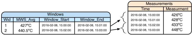
Figure 2: Schema for storing archived streams and MWSs

We will now discuss, using an example, the Materialised Window Signatures technique for hybrid operations. Consider the relational schema depicted in Fig. 2 which is adopted for storing archived streams and performing hybrid operations on them. The relational table Measurements represents the archived part of the stream and stores the temporal identifier (Time) of each measurement and the actual values (attribute Measurement). The relational table Windows identifies the windows that have appeared up till now based on the existing window-mechanism. It contains a unique identifier for each window (Wid) and the attributes that determine its starting and ending points (Window_Start, Window_End). The necessary indices that will facilitate the complex analytic computations are materialised. The depicted schema is flexible to query changes since it separates the windowing mechanism —which is query dependent— from the actual measurements.

In order to accelerate analytical tasks that include hybrid operations over archived streams, we facilitate precompution of frequently requested aggregates on each archived window. We name these precomputed summarisations as Materialised Window Signatures (MWSs). These MWSs are calculated when past windows are stored in the backend and are later utilised while performing complex calculations between these windows and a live stream. The summarisation values are determined by the analytics under consideration. E.g., for the computation of the Pearson correlation, we precompute the average value and standard deviation on each archived window measurements; for the cosine similarity, we precompute the Euclidean norm of each archived window; for finding the absolute difference between the average values of the current and the archived windows, we precompute the average value, etc.

The selected MWSs are stored in the Windows relation with the use of additional columns. In Fig. 2 we see the MWS summary for the $\mathtt{avg}$ aggregate function being included in the relation as an attribute termed $\mathtt{MWS\_Avg}$. The application can easily modify the schema of this relation in order to add or drop MWSs, depending on the analytical workload.

When performing hybrid operations between the current and archived windows, some analytic operations can be directly computed based on their MWS values with no need to access the actual archived measurements. This provides significant benefits as it removes the need to perform a costly join operation between the live stream and the, potentially very large, Measurements relation. On the opposite, for calculations such as the Pearson correlation coefficient and the cosine similarity measures, we need to perform calculations that require the archived measurements as well, e.g., for computing cross-correlations or inner-products. Nevertheless, the MWS approach allows us to avoid recomputing some of the information on each archived window such as its avg value and deviation for the Pearson correlation coefficient, and the Euclidean norm of each archived window for the cosine similarity measure. Moreover, in case when there is a selective additional filter on the query (such as the avg value exceeds a threshold), by creating an index on the $\mathtt{MWS}$ attributes, we can often exclude large portions of the archived measurements from consideration, by taking advantage of the underlying index.

3 Implementation

In this section we discuss our system that implements the OBDA extensions proposed in Sec. 2. In Fig. 3 (Left), we present a general architecture of our system. On the application level one can formulate STARQL queries over analytics-aware ontologies and pass them to the query compilation module that performs query rewriting, unfolding, and optimisation. Query compilation components can access relevant information in the ontology for query rewriting, mappings for query unfolding, and source specifications for optimisation of data queries. Compiled data queries are sent to a query execution layer that performs distributed query evaluation over streaming and static data, post-processes query answers, and sends them back to applications. In the following we will discuss two main components of the system, namely, our dedicated STARQL2SQL^⊕ translator that turns STARQL queries to SQL^⊕ queries, and our native data-stream management system ExaStream that is in charge of data query optimisation and distributed query evaluation.

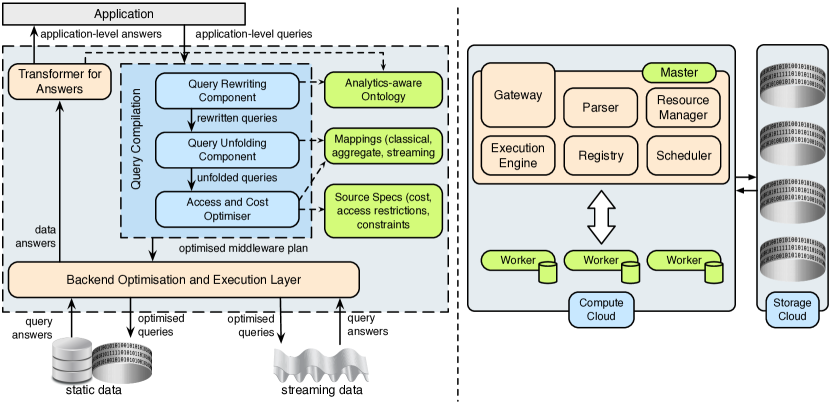
Figure 3: (Left) General architecture. (Right) Distributed stream engine of ExaStream

3.0.1 STARQL to SQL^⊕ Translator.

Our translator consists of several modules for transformation of various query components and we now give some highlights on how it works. The translator starts by turning the window operator of the input STARQL query and this results in a slidingWindowView on the backend system that consists of columns for defining windowID (as in Fig. 2) and dataGraphID based on the incoming data tuples. Our underlying data-stream management system ExaStream already provides user defined functions (UDFs) that automatically create the desired streaming views, e.g., the timeSlidingWindow function as discussed below in the ExaStream part of the section.

The second important transformation step that we implemented is the transformation of the STARQL HAVING clause. In particular, we normalise the HAVING clause into a relational algebra normal form (RANF) and apply the described slicing technique illustrated in Sec. 2.3.3, where we unfold each state of the temporal sequence into slices of the slidingWindowView. For the rewriting and unfolding of each slice, we make use of available tools using the OBDA paradigm in the static case, i.e., the Ontop framework [5]. After unfolding, we join all states together based on their temporal relations given in the HAVING sequence.

3.0.2 ExaStream Data-Stream Management System.

Data queries produced by the STARQL2SQL^⊕ translation, are handled by ExaStream which is embedded in Exareme, a system for elastic large-scale dataflow processing in the cloud [27, 28].

ExaStream is built as a streaming extension of the SQLite database engine, taking advantage of existing Database Management technologies and optimisations. It provides the declarative language SQL^⊕ for querying data streams and relations. SQL^⊕ extends SQL with UDFs that incorporate the algorithmic logic for transforming SQLite into a Data Stream Management Systems (DSMS). E.g., the timeSlidingWindow operator groups tuples from the same time window and associates them with a unique window id. In contrast to other DSMSs, the user does not need to consider low-level details of query execution. Instead, the system’s query planner is responsible for choosing an optimal plan depending on the query, the available stream/static data sources, and the execution environment.

ExaStream system exploits parallelism in order to accelerate the process of analytical tasks over thousands of stream and static sources. It manages an elastic cloud infrastructure and dynamically distributes queries and data (including both streams and static tables) to multiple worker nodes that process them in parallel. The architecture of ExaStream’s distributed stream engine is presented in Fig. 3 (Right). One can see that queries are registered through the Asynchronous Gateway Server. Each registered query passes through the ExaStream parser and then is fed to the Scheduler module. The Scheduler places the stream and relational operators on worker nodes based on the node’s load. These operators are executed by a Stream Engine instance running on each node.

4 Evaluation

The aim of our evaluation is to study how the MWS technique and query distribution to multiple workers accelerate the overall execution time of analytic queries that correlate a live stream with multiple archived stream records.

4.0.1 Evaluation Setting.

We deployed our system to the Okeanos Cloud Infrastructure (www.okeanos.grnet.gr/) and used up to $16$ virtual machines (VMs) each having a 2.66 GHz processor with 4GB of main memory. We used streaming and static data that contains measurements produced by $100,000$ thermocouple sensors installed in 950 Siemens power generating turbines. For our experiments, we used three test queries calculating the similarity between the current live stream window and 100,000 archived ones. In each of the test queries we fixed the window size to 1 hour which corresponds to 60 tuples of measurements per window. The first query is based on the one from our running example (see Fig. 1) which we modified so that it can correlate a live stream with a varying number of archived streams. Recall that this query evaluates window measurements similarity based on the Pearson correlation. The other two queries are variations of the first one where, instead of the Pearson correlation, they compute similarity based on either the average or the minimum values within a window. We defined such similarities between vectors (of measurements) $\vec{w}$ and $\vec{v}$ as follows: $|\text{avg}(\vec{w})-\text{avg}(\vec{v})|<10^{\circ}C$ and $|\text{min}(\vec{w})-\text{min}(\vec{v})|<10^{\circ}C$. The archived streams windows are stored in the Measurements relation, against which the current stream is compared.

4.0.2 MWS Optimisation.

This set of experiments is devised to show how the MWS optimisation affects the query’s response time. We executed each of the three test queries on a single VM-worker with and without the MWS optimisation. In Fig. 4 (Left) we present the results of our experiments. The reported time is the average of 15 consecutive live-stream execution cycles. The horizontal axis displays the three test queries with and without the MWS optimisation, while the vertical axis measures the time it takes to process 1 live-stream window against all the archived ones. This time is divided to the time it takes to join the live stream and the Measurements relation and the time it takes to perform the actual computations. Observe that the MWS optimisation reduces the time for the Pearson query by 8.18%. This is attributed to the fact that some computations (such as the avg and standard deviation values) are already available in the Winodws relation and are, thus, omitted. Nevertheless, the join operation between the live stream and the very large Measurements relation that takes 69.58% of the overall query execution time can not be avoided. For the other two queries, we not only reduce the CPU overhead of the query, but the optimiser further prunes this join from the query plan as it is no longer necessary. Thus, for these queries, the benefits of the MWS technique are substantial.

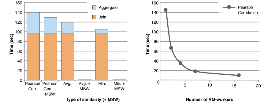
Figure 4: (Left) Effect of MWS optimisation (Right) Effect of intra-query parallelism

4.0.3 Intra-query Parallelism.

Since the MWS optimisation substantially accelerates query execution for the two test queries that rely on average and minimum similarities, query distribution would not offer extra benefit, and thus these queries were not used in the second experiment. For complex analytics such as the Pearson correlation that necessitates access to the archived windows, the ExaStream backend permits us to accelerate queries by distributing the load among multiple worker nodes. In the second experiment we use the same setting as before for the Pearson computation without the MWS technique, but we vary this time the number of available workers from 1 to 16. In Fig. 4 (Right), one can observe a significant decrease in the overall query execution time as the number of VM-workers increases. ExaStream distributes the Measurements relation between different worker nodes. Each node computes the Pearson coefficient between its subset of archived measurements and the live stream. As the number of archived windows is much greater than the number of available workers, intra-query parallelism results is significant decrease to the time required to perform the join operation.

To conclude this section, we note that MWSs gave us significant improvements of query execution time for all test queries and parallelism would be essential in the cases where MWSs do not help in avoiding the high cost of query joins since it allows to run the join computation in parallel. Due to space limitations, we do not include an experiment examining the query execution times w.r.t. the number of archived windows. Nevertheless, based on our observations, scaling up the number of archived windows by a factor of $n$ has about the same effect as scaling down the number of workers by $\nicefrac{{1}}{{n}}$.

5 Related Work

5.0.1 OBDA System.

Our proposed approach extends existing OBDA systems since they either assume that data is in (static) relational DBs, e.g [11, 5], or streaming, e.g., [8, 9], but not of both kinds. Moreover, we are different from existing solutions for unified processing of streaming and static semantic data e.g. [29], since they assume that data is natively in RDF while we assume that the data is relational and mapped to RDF.

5.0.2 Ontology language.

The semantic similarities of $\textit{DL-Lite}_{\cal A}^{\sf agg}$ to other works have been covered in Sec. 2. Syntactically, the aggregate concepts of $\textit{DL-Lite}_{\cal A}^{\sf agg}$ have counterpart concepts, named local range restrictions (denoted by $\forall F.T$) in $\textit{DL-Lite}_{\cal A}$ [30]. However, for purposes of rewritability, these concepts are not allowed on the left-hand side of inclusion axioms as we have done for $\textit{DL-Lite}_{\cal A}^{\sf agg}$, but only in a very restrictive semantic/syntactic way. The semantics of $\textit{DL-Lite}_{\cal A}^{\sf agg}$ for aggregate concepts is very similar to the epistemic semantics proposed in [16] for evaluating conjunctive queries involving aggregate functions. A different semantics based on minimality has been considered in [17]. Concepts based on aggregates functions were considered in [31] for languages $\cal ALC$ and $\cal EL$ with concrete domains, but they did not study the problem of query answering.

5.0.3 Query language.

While already several approaches for RDF stream reasoning engines do exist, e.g., CSPARQL [32], RSP-QL [33] or CQELS [34], only one of them supports an ontology based data access approach, namely SPARQLstream [8]. In comparison to this approach, which also uses a native inclusion of aggregation functions, STARQL offers more advanced user defined functions from the backend system like Pearson correlation.

5.0.4 Data Stream Management System.

One of the leading edges in database management systems is to extend the relational model to support for continuous queries based on declarative languages analogous to SQL. Following this approach, systems such as TelegraphCQ [35], STREAM [36], and Aurora [37] take advantage of existing Database Management technologies, optimisations, and implementations developed over 30 years of research. In the era of big data and cloud computing, a different class of DSMS has emerged. Systems such as Storm and Flink offer an API that allows the user to submit dataflows of user defined operators. ExaStream unifies these two different approaches by allowing to describe in a declarative way complex dataflows of (possibly user-defined) operators. Moreover, the Materialised Window Signature summarisation, implemented in ExaStream, is inspired from data warehousing techniques for maintaining selected aggregates on stored datasets [38, gray1997data]. We adjusted these technique for complex analytics that blend streaming with static data.

6 Conclusion, Lessons Learned, and Future Work

We see our work as a first step towards the development of a solid theory and new full-fledged systems in the space of analytics-aware ontology-based access to data that is stored in different formats such as static relational, streaming, etc. To this end we proposed ontology, query, and mapping languages that are capable of supporting analytical tasks common for Siemens turbine diagnostics. Moreover, we developed a number of backend optimisation techniques that allow such tasks to be accomplished in reasonable time as we have demonstrated on large scale Siemens data.

The lessons we have learned so far are the encouraging evaluation results over the Siemens turbine data (presented in Section 4). Since our work is a part of an ongoing project that involves Siemens, we plan to continue implementation and then deployment of our solution in Siemens. This will give us an opportunity to do further performance evaluation as well as to conduct user studies.

Finally, there is a number of important further research directions that we plan to explore. On the side of analytics-aware ontologies, since bag semantics is natural and important in analytical tasks, we see a need in exploring bag instead of set semantics for ontologies. On the side of analytics-aware queries, an important further direction is to align them with the terminology of the W3C RDF Data Cube Vocabulary and to provide additional optimisations after the alignment. As for query optimisation techniques, exploring approximation algorithms for fast computation of complex analytics between live and archived streams is particularly important. That is because these algorithms usually provide quality guarantees about the results and in the average case require much less computation. Thus, we intend to examine their effectiveness in combination with the MWS approach. Another interesting backend optimisation relates to the pre-computation of the appropriate structures that will accelerate the aggregate-query execution, e.g. materialised views and database indexes. We intend to examine refined optimisation techniques that combine information on the OBDA layer with building of the appropriate structures on our DSMS (or database engine).

References

- [1] Calvanese, D., Giacomo, G., Lembo, D.: Ontologies and Databases: The DL-Lite Approach. In: Reas. Web. (2009)
- [2] Bizer, C., Seaborne, A.: D2RQ-Treating Non-RDF Databases as Virtual RDF Graphs. In: ISWC. (2004)
- [3] Calvanese, D., De Giacomo, G., Lembo, D., Lenzerini, M., Poggi, A., Rodriguez-Muro, M., Rosati, R., Ruzzi, M., Savo, D.F.: The MASTRO System for Ontology-Based Data Access. Semantic Web 2(1) (2011) 43–53
- [4] Priyatna, F., Corcho, O., Sequeda, J.: Formalisation and Experiences of R2RML-Based SPARQL to SQL Query Translation Using Morph. In: WWW. (2014) 479–490
- [5] Rodriguez-Muro, M., Kontchakov, R., Zakharyaschev, M.: Ontology-Based Data Access: Ontop of Databases. In: ISWC. (2013) 558–573
- [6] Munir, K., Odeh, M., McClatchey, R.: Ontology-Driven Relational Query Formulation Using the Semantic and Assertional Capabilities of OWL-DL. Knowl.-Based Syst. 35 (2012) 144–159
- [7] Sequeda, J., Miranker, D.P.: Ultrawrap: SPARQL Execution on Relational Data. JWS 22 (2013) 19–39
- [8] Calbimonte, J., Corcho, Ó., Gray, A.J.G.: Enabling ontology-based access to streaming data sources. In: ISWC. (2010) 96–111
- [9] Fischer, L., Scharrenbach, T., Bernstein, A.: Scalable linked data stream processing via network-aware workload scheduling. In: SSWKBS@ISWC. (2013) 81–96
- [10] Calvanese, D., Liuzzo, P., Mosca, A., Remesal, J., Rezk, M., Rull, G.: Ontology-based Data Integration in EPNet: Production and Distribution of Food During the Roman Empire. Eng. Appl. of AI 51 (2016) 212–229
- [11] Civili, C., Console, M., De Giacomo, G., Lembo, D., Lenzerini, M., Lepore, L., Mancini, R., Poggi, A., Rosati, R., Ruzzi, M., Santarelli, V., Savo, D.F.: MASTRO STUDIO: managing ontology-based data access applications. PVLDB 6(12) (2013) 1314–1317
- [12] Kharlamov, E., Hovland, D., Jiménez-Ruiz, E., Pinkel, D.L.C., Rezk, M., Skjæveland, M.G., Thorstensen, E., Xiao, G., Zheleznyakov, D., Bjørge, E., Horrocks, I.: Enabling Ontology Based Access at an Oil and Gas Company Statoil. In: ISWC. (2015)
- [13] Kharlamov, E., Solomakhina, N., Özçep, Ö.L., Zheleznyakov, D., Hubauer, T., Lamparter, S., Roshchin, M., Soylu, A., Watson, S.: How Semantic Technologies Can Enhance Data Access at Siemens Energy. In: ISWC. (2014)
- [14] Rodrıguez-Muro, M., Calvanese, D.: High Performance Query Answering Over DL-Lite Ontologies. In: KR. (2012)
- [15] Lutz, C., Seylan, I., Wolter, F.: Mixing Open and Closed World Assumption in Ontology-Based Data Access: Non-Uniform Data Complexity. In: DL. (2012)
- [16] Calvanese, D., Kharlamov, E., Nutt, W., Thorne, C.: Aggregate Queries Over Ontologies. In: ONISW. (2008) 97–104
- [17] Kostylev, E.V., Reutter, J.L.: Complexity of Answering Counting Aggregate Queries Over DL-Lite. J. of Web Sem. 33 (2015) 94–111
- [18] Özçep, Özgür., Möller, R., Neuenstadt, C.: A Stream-Temporal Query Language for Ontology Based Data Access. In: KI. (2014) 183–194
- [19] Arasu, A., Babu, S., Widom, J.: The cql continuous query language: Semantic foundations and query execution. VLDBJ 15(2) (2006) 121–142
- [20] Kharlamov, E., Brandt, S., Giese, M., Jiménez-Ruiz, E., Kotidis, Y., Lamparter, S., Mailis, T., Neuenstadt, C., Özçep, Ö.L., Pinkel, C., Soylu, A., Svingos, C., Zheleznyakov, D., Horrocks, I., Ioannidis, Y.E., Möller, R., Waaler, A.: Enabling semantic access to static and streaming distributed data with optique: demo. In: DEBS Demo. (2016) 350–353
- [21] Kharlamov, E., Brandt, S., Jimenez-Ruiz, E., Kotidis, Y., Lamparter, S., Mailis, T., Neuenstadt, C., Özçep, O., Pinkel, C., Svingos, C., Zheleznyakov, D., Horrocks, I., Ioannidis, Y., Möller, R.: Ontology-Based Integration of Streaming and Static Relational Data with Optique. SIGMOD demo (2016)
- [22] Kharlamov, E., Brandt, S., Giese, M., Jiménez-Ruiz, E., Lamparter, S., Neuenstadt, C., Özçep, Ö.L., Pinkel, C., Soylu, A., Zheleznyakov, D., Roshchin, M., Watson, S., Horrocks, I.: Semantic access to siemens streaming data: the optique way. In: ISWC. (2015)
- [23] Kharlamov, E., Jiménez-Ruiz, E., Pinkel, C., Rezk, M., Skjæveland, M.G., Soylu, A., Xiao, G., Zheleznyakov, D., Giese, M., Horrocks, I., Waaler, A.: Optique: Ontology-based data access platform. In: ISWC P&D. (2015)
- [24] Kharlamov, E., Jiménez-Ruiz, E., Zheleznyakov, D., Bilidas, D., Giese, M., Haase, P., Horrocks, I., Kllapi, H., Koubarakis, M., Özçep, Ö.L., Rodriguez-Muro, M., Rosati, R., Schmidt, M., Schlatte, R., Soylu, A., Waaler, A.: Optique: Towards OBDA Systems for Industry. In: ESWC (Selected Papers). (2013) 125–140
- [25] Kharlamov, E., Giese, M., Jiménez-Ruiz, E., Skjæveland, M.G., Soylu, A., Zheleznyakov, D., Bagosi, T., Console, M., Haase, P., Horrocks, I., Marciuska, S., Pinkel, C., Rodriguez-Muro, M., Ruzzi, M., Santarelli, V., Savo, D.F., Sengupta, K., Schmidt, M., Thorstensen, E., Trame, J., Waaler, A.: Optique 1.0: Semantic Access to Big Data: The Case of Norwegian Petroleum Directorate FactPages. In: ISWC Posters & Demos. (2013)
- [26] Neuenstadt, C., Möller, R., Özçep, Özgür.L.: OBDA for Temporal Querying and Streams with STARQL. In: HiDeSt. (2015)
- [27] Tsangaris, M.M., Kakaletris, G., Kllapi, H., Papanikos, G., Pentaris, F., Polydoras, P., Sitaridi, E., Stoumpos, V., Ioannidis, Y.E.: Dataflow Processing and Optimization on Grid and Cloud Infrastructures. IEEE Data Eng. Bull. 32(1) (2009) 67–74
- [28] Kllapi, H., Sakkos, P., Delis, A., Gunopulos, D., Ioannidis, Y.: Elastic Processing of Analytical Query Workloads on IaaS Clouds. In: arXiv. (2015)
- [29] Phuoc, D.L., Dao-Tran, M., Parreira, J.X., Hauswirth, M.: A Native and Adaptive Approach for Unified Processing of Linked Streams and Linked Data. In: ISWC. (2011) 370–388
- [30] Artale, A., Ryzhikov, V., Kontchakov, R.: DL-Lite with Attributes and Datatypes. In: ECAI. (2012) 61–66
- [31] Baader, F., Sattler, U.: Description logics with aggregates and concrete domains. IS 28(8) (2003) 979–1004
- [32] Barbieri, D.F., Braga, D., Ceri, S., Valle, E.D., Grossniklaus, M.: C-SPARQL: A Continuous Query Language for RDF Data Streams. Int. J. Sem. Computing 4(1) (2010) 3–25
- [33] Aglio, D.D., Valle, E.D., Calbimonte, J.P., Corcho, O.: RSp-ql semantics: A unifying query model to explain heterogeneity of rdf stream processing systems. IJSWIS 10(4) (2015)
- [34] Le-Phuoc, D., Dao-Tran, M., Pham, M.D., Boncz, P., Eiter, T., Fink, M.: Linked Stream Data Processing Engines: Facts and Figures. In: ISWC. (2012) 300–312
- [35] Chandrasekaran, S., Cooper, O., Deshpande, A., Franklin, M.J., Hellerstein, J.M., Hong, W., Krishnamurthy, S., Madden, S.R., Reiss, F., Shah, M.A.: TelegraphCQ: Continuous Dataflow Processing. In: SIGMOD. (2003) 668–668
- [36] Arasu, A., Babcock, B., Babu, S., Datar, M., Ito, K., Nishizawa, I., Rosenstein, J., Widom, J.: STREAM: the stanford stream data manager. In: SIGMOD. (2003) 665
- [37] Abadi, D., Carney, D., Cetintemel, U., Cherniack, M., Convey, C., Erwin, C., Galvez, E., Hatoun, M., Maskey, A., Rasin, A., et al.: Aurora: A Data Stream Management System. In: SIGMOD. (2003) 666–666
- [38] Kotidis, Y., Roussopoulos, N.: DynaMat: A Dynamic View Management System for Data Warehouses. In: SIGMOD. (1999) 371–382