Adiabatic regularization of power spectra in nonminimally coupled chaotic inflation

Abstract

We investigate the effect of adiabatic regularization on both the tensor- and scalar-perturbation power spectra in nonminimally coupled chaotic inflation. Similar to that of the minimally coupled general single-field inflation, we find that the subtraction term is suppressed by an exponentially decaying factor involving the number of $e$-folds. By following the subtraction term long enough beyond horizon crossing, the regularized power spectrum tends to the “bare” power spectrum. This study justifies the use of the unregularized (“bare”) power spectrum in standard calculations.

1 Introduction

Cosmic inflation [1, 2, 3, 4, 5, 6] found its place in modern cosmology as a solution to the horizon and flatness problems and an explanation for the origin of primordial cosmological perturbations [7, 8] that served as seeds for the large-scale structures (e.g., galaxies and clusters of galaxies) nowadays constituting the Universe. Like any other system of ideas intended to explain nature or a part thereof, this theory has to satisfy at least the two-pronged requirement of science namely, self consistency and agreement with experiment. The latter requires a theory to explain existing measurement results before its inception and predict values of physical observables (e.g., in the case of inflation, non-Gaussianity, tensor-to-scalar ratio, spectral tilt, etc. [9, 10]). On the other hand, self-consistency ensures that pathways of ideas within the framework of the theory do not lead to illogical contradiction and problematic calculation results such as those involving non-removable divergences. On this side, inflation must pass checks involving loop corrections [11, 12], divergences in predicted physical observables [13], and the more general question of renormalization (e.g., see Ref. [14]).

In this work, we focus on the side of self-consistency and investigate the effect of removing infinities from the two-point functions of scalar and tensor perturbations, on their power spectra. In particular, we consider the adiabatic regularization [13, 15, 16, 17] of the power spectra for the perturbations in nonminimally coupled single-field inflation [18, 19, 20, 21, 22] (see Sec. 2 for the details of the setup). It is an extension/generalization of the work of Urakawa and Starobinsky [23] involving the adiabatic regularization of the power spectra in the canonical single-field inflation. In our previous work [24], we performed the extension/generalization of their study along a different pathway including cases where the speed of sound $c_{s}^{2},$ is not constant (that is, general single-field inflation, or, as usually referred to in the literature, k-inflation,) but maintained the minimal-coupling aspect of the theory (see Fig. 1). This time, adding a nonminimal coupling term on top of the canonical case ($c_{s}^{2}=1$), we wish to determine if adiabatic regularization will significantly modify the power spectrum contrary to what was found by Urakawa and Starobinsky and in our extension to the general single-field inflation of their study.

Figure 1: Generalizations of the canonical inflation. The canonical case involves the Lagrangian $\mathcal{L}=\frac{1}{2}M_{\text{Pl}}^{2}R+X-V(\phi)$, where $M_{\text{Pl}},\,R,\,X,$ and $V$ are the Planck mass, Ricci scalar, kinetic term, and potential term respectively. On the one hand, nonminimally coupled chaotic inflation (right hand most box) involves the addition of nonminimal coupling (N.M.C.) term to the canonical case. On the other hand, $k$-inflation involves a Lagrangian that is a general functional of $X$ and $\phi$; that is, $P(X,\phi)$.

Before we proceed with the calculation to fulfill this aim, it is good to shed some light on adiabatic regularization in the context of the problem we are dealing in this work. The two-point function of the gauge-invariant scalar perturbation $\mathcal{R}$ [25] can be written as

$$\langle\mathcal{R}(\tau,\mathbf{x})\mathcal{R}(\tau,\mathbf{y})\rangle =\int\frac{\text{d}k}{k}\frac{\sin(k|\mathbf{x}-\mathbf{y}|)}{k|\mathbf{x}-\mathbf{y}|}\Delta^{2}_{\mathcal{R}}(k,\tau),$$ (1.1)

where $\tau$ is the conformal time, $(\mathbf{x},\mathbf{y})$ are pairs of position vectors, $k$ is the wavenumber, and $\Delta^{2}_{\mathcal{R}}$ is the dimensionless power spectrum given by

$$\Delta_{\mathcal{R}}^{2}(k,\tau)=\frac{k^{3}}{2\pi^{2}}\big{|}\mathcal{R}_{k}(\tau)\big{|}^{2},$$ (1.2)

with the subscript $k$ in $\mathcal{R}_{k}$ indicating momentum space. (Similar expression holds for the tensor perturbation.) The adiabatic condition [13, 26] tells us that $|\mathcal{R}_{k}(\tau)|$ scales as $1/k$ for large $k$ leading to $\Delta^{2}_{\mathcal{R}}\sim k^{2}$. It follows that in the coincidence limit, $\mathbf{x}\,\rightarrow\,\mathbf{y}$, the integral diverges. As applied to this scenario, adiabatic regularization is a method of systematically subtracting out terms in the integrand to yield a finite two-point function, subject to the assumption that the adiabatic condition holds. Such a subtraction scheme is correspondingly reflected in the power spectrum. One may then see that the physical power spectrum is the difference between the “bare” and the corresponding subtraction term.

There is a disagreement about this viewpoint. Parker and his collaborators [27, 28, 29] advocate the need for adiabatic regularization and claim that it could significantly modify the power spectrum (with both the “bare” and the subtraction term evaluated before or at the moment of horizon crossing), producing expressions not in accord with the “bare” power spectrum used in standard calculations. Some other people casted some doubt on the necessity of this subtraction scheme based on the claims that (a) the regularised power spectrum can become negative when one goes beyond the minimal subtraction scheme [30] and (b) in the far infrared regime, the adiabatic expansion is no longer valid [31]. Moreover, in the review paper of Bastero-Gil et al. [32], the authors argued that the cosmic microwave background (CMB) anisotropy variable $C_{l}$ depends on the inflaton two-point function evaluated at $\mathbf{x}\neq\mathbf{y}$; thus, practically avoiding the divergence in (1.1).

We adopt a position that adiabatic regularization may be necessary and its application to calculation of physical observables produces physically consistent result. In so taking this position, we wish not to devote this paper as an argumentative defense of such position. What we do here is leave some words in favor of our chosen side and focus on the main subject of this work; that is, the application of adiabatic regularization to the calculation of power spectra. First, the coincidence limit $\mathbf{x}\,\rightarrow\,\mathbf{y}$ is a mathematical possibility that cannot be avoided by the mere existence of physical circumstances where such a limit may not hold. Furthermore, when one considers potentials involving self interaction or the energy-momentum tensor, the divergences are certainly inevitable. Second, the adiabatic regularization includes as its prescription that the subtraction scheme be minimal; rather informally, those terms producing infinity should be the only subjects of regularization to remove them. Since the adiabatic expansion say, of $\mathcal{R}$, is in general, not convergent but only asymptotic [13], such a prescription prevents a given quantity—one whose mathematical sickness we want to cure in the first place—from becoming unphysical or ill-behaved (e.g., power spectrum becoming negative). Third and last, determining the definite cut on the value of the spectrum of $k$ as to when adiabatic regularization should be or should not be performed would seem to introduce an unnecessary complication to this method whenever quantities in momentum space are considered. If only to tame the doubts casted by Durrer et al. [31] that the adiabatic expansion may not be valid in the far infrared limit, we note that there are good indications that the subtraction term becomes negligible for the quantities involving superhorizon modes (see for instance, Refs. [23, 24]).

In this work as in our previous work [24], we follow the track laid down by Urakawa and Starobinsky [23]. We perform adiabatic regularization using the minimal subtraction scheme and follow the subtraction term long after the first horizon crossing during inflation. As what they found out, the subtraction term exponentially decays with the number of $e$-folds, resulting to the standard expression; i.e., the regularized power spectrum tends to the “bare” power spectrum. As already mentioned above, we have done the same for the extension to the minimally coupled general single-field inflation. This study showed that apart from cases that may significantly deviate from the condition of scale invariance, the subtraction “leads to no difference in the power spectrum” [24]. It is then our aim in this investigation to see if the same holds for the case of nonminimally coupled inflation.

This paper is organized as follows. In Sec. 2, we provide the setup for nonminimally coupled chaotic inflation. In so doing, we state the action and the background equations necessary for our analysis and calculations. In Sec. 3, perturbations are introduced about the FLRW metric and the “bare” power spectra for these perturbations (scalar and tensor) are calculated up to first order in the slow-roll parameters. After this, we compute the subtraction terms (also up to first order in the slow-roll parameters) and perform adiabatic regularization of the power spectra in Sec. 4. Following this, we justify the use of both the Einstein and Jordan frames in our calculation in Sec. 5. In the last section, we state our conclusion and future prospects about further generalizing this work to cases involving non-constant speed of sound, higher-order corrections to the power spectrum, and gravity beyond general relativity.

2 Set up: Nonminimal Chaotic Inflation

Nonminimal chaotic inflation was proposed by Fakir and Unruh [18] (see also, Ref. [19]) to avoid the fine-tuning problem associated with the coupling constant $\lambda$ in chaotic inflation involving the potential $\lambda\phi^{4},$ where $\phi$ is the inflaton field. Since its conception in 1988, several other papers followed covering (a) a rigorous evaluation of the density perturbation amplitude (1991) [20], (b) constraints on physical observables such as the tensor-to-scalar ratio and spectral tilt (1999) [21], (c) loop corrections (2010, 2015) [34, 35], (d) observational consequences with the addition of a quadratic potential term (2011) [33], and (e) non-Gaussianity (2011) [36], among others. It is thus, an intensively studied model consistent with the current observational constraints [9, 10].

We consider in this work the action given by

$$S =\frac{1}{2}\int\sqrt{-g}\,\text{d}^{4}x\Big{[}M_{\text{Pl}}^{2}f(\phi)R-g^{\mu\nu}\nabla_{\mu}\phi\nabla_{\nu}\phi-2V(\phi)\Big{]},$$ (2.1)

where $g_{\mu\nu}$ is the metric, $R$ is the Ricci scalar, $V(\phi)$ is the potential, and $f(\phi)\equiv 1+h(\phi)$ with $M_{\text{Pl}}^{2}$ as the Planck mass (squared) that from hereon, take as unity for brevity. Furthermore, given $\xi$ as the nonminimal coupling parameter, we take

$$h(\phi)=\frac{\xi\phi^{2}}{M_{\text{Pl}}^{2}}=\xi\phi^{2}\quad\text{and}\quad V(\phi)=\frac{\lambda}{4}\phi^{4},$$ (2.2)

corresponding to the nonminimal chaotic inflation model well-investigated in the references cited above and the references therein. This choice allows us to have a fixed model with well-known characteristics that we can exploit in our analysis. However, as it may be beneficial for future study of a more general case, we keep the symbol $h(\phi)$ and $V(\phi)$ in our calculations. The limit to the specific case given by (2.2) is considered in the final expression for the regularized power spectrum and in the discussion of some other quantities where there may be a need to have a fixed model.

For the Friedmann-Lemaître-Robertson-Walker (FLRW) metric describing the background spacetime for the action above,

$$\text{d}s^{2}=-\text{d}t^{2}+a^{2}(t)\delta_{ij}\text{d}x^{i}\text{d}x^{j},$$ (2.3)

where $a(t)$ is the scale factor, the equation of motion (EOM) for $\phi$ reads

$$\ddot{\phi}+3H\dot{\phi}+\bigg{(}1+\frac{3}{2}\frac{h_{\phi}^{2}}{f}\bigg{)}^{-1}V_{\phi}+\frac{1}{2}\frac{h_{\phi}}{f}(1+3h_{\phi\phi})\bigg{(}1+\frac{3}{2}\frac{h_{\phi}^{2}}{f}\bigg{)}^{-1}\dot{\phi}^{2}$$

$$\qquad-\,\frac{2h_{\phi}}{f}\bigg{(}1+\frac{3}{2}\frac{h_{\phi}^{2}}{f}\bigg{)}^{-1}V=0,$$ (2.4)

where the overdot means differentiation with respect to the coordinate time $t$, and the subscript $\phi$ denotes derivative with respect to $\phi$. It is straightforward to verify that this equation reduces to the EOM for $\phi$ given in the paper of Komatsu and Futamase [21] for the case specified in (2.2). In addition to this, the Friedmann equation derived from the Einstein equation reads

$$H^{2}=\frac{\rho}{3}=\frac{1}{3f}\Big{(}\tfrac{1}{2}\,\dot{\phi}^{2}+V-3\dot{h}H\Big{)},$$ (2.5)

where $H\equiv\dot{a}/a$, is the Hubble parameter.

The variation of the action with respect to $g_{\mu\nu}$ leads to the expression for the conserved energy-momentum tensor $T^{\mu}{}_{\nu}=\text{diag}(-\rho,p,p,p)$, with $\rho$ and $p$ being the background energy density and pressure respectively.

$$\rho =\frac{1}{f}\Big{(}\tfrac{1}{2}\,\dot{\phi}^{2}+V-3\dot{h}H\Big{)},$$

$$p =\frac{1}{f}\Big{(}\tfrac{1}{2}\,\dot{\phi}^{2}-V+2\dot{h}H+\ddot{h}\Big{)}.$$ (2.6)

Since $\dot{H}=-\frac{1}{2}(\rho+p)$ and the slow-roll parameter $\epsilon=-\dot{H}/H^{2}$ by definition, we find

$$\epsilon=\frac{1}{f}\bigg{(}\frac{\dot{\phi}^{2}}{2H^{2}}-\frac{\dot{h}}{2H}+\frac{\ddot{h}}{2H^{2}}\bigg{)}.$$ (2.7)

For the slow-roll (chaotic) inflation that we assume in this article, $|\epsilon|\ll 1$, implying the conditions $\dot{\phi}^{2}/fH^{2},\,|\dot{h}/fH|,$ $|\ddot{h}/fH^{2}|\ll 1$. These inequalities are satisfied by the inflationary solution in the case where $h(\phi)=\xi\phi^{2}$ and $V(\phi)=(\lambda/4)\phi^{4}$, with $h\gg 1$. In particular, the Friedmann equation reads [18, 21],

$$H^{2}=\frac{\lambda h}{12\xi^{2}},\quad\text{with}\quad\frac{\dot{h}}{H}=-\frac{8\xi}{1+6\xi},$$ (2.8)

as a consequence of standard slow-roll assumption, the condition $h\gg 1$, and the equation of motion for $\phi$. Inflation ends when $\epsilon=1$ corresponding to $h=\xi\phi^{2}\sim\mathcal{O}(1)$ [18].

3 The “bare” Power Spectrum

With the background equations in place, we now consider the perturbations and proceed to calculate their power spectra. In our calculations, we use the comoving gauge where the inflaton fluctuation vanishes ($\delta\phi=0$) and the three-dimensional metric takes the form

$$g_{ij} =a^{2}(t)e^{2\mathcal{R}(\mathbf{x},t)}\left(e^{\gamma(\mathbf{x},t)}\right)_{ij},\quad\partial^{i}\gamma_{ij}=\gamma^{i}{}_{i}=0,$$ (3.1)

where $\mathcal{R}$ is the gauge-invariant (scalar) curvature perturbation and $\gamma_{ij}$ is the transverse traceless tensor perturbation. Including these perturbations about the homogeneous and isotropic spacetime described by the FLRW metric (2.3), the metric in the Arnowitt-Deser-Misner (ADM) formulation (that we use here,) can be written as [38, 39]

$$\text{d}s^{2} =-N^{2}\text{d}t^{2}+g_{ij}(\text{d}x^{i}+N^{i}\text{d}t)(\text{d}x^{j}+N^{j}\text{d}t),$$ (3.2)

where $N$ and $N^{i}$ are the lapse and shift functions respectively.

Using the metric above and the comoving gauge, the computation of the power spectrum for $\mathcal{R}$ proceeds by the decomposition of the action as $S=S^{(0)}+S^{(2)}+S^{(3)}+\cdots,$ where the quantity n in $S^{(n)}$ indicates the order with respect to $\mathcal{R}$ (see for instance, Refs. [40, 36]). The segment $S^{(2)}$ corresponds to the power spectrum. In the minimal case, the EOM called the Mukhanov-Sasaki equation, derived from $\bar{S}^{(2)}$ reads

$$\bar{v}_{k}^{\prime\prime}+\left(k^{2}-\frac{\bar{z}^{\prime\prime}}{\bar{z}}\right)\bar{v}_{k}=0,$$ (3.3)

where the overbar signifies minimal coupling, the subscript $k$ indicates momentum space, the prime symbol means differentiation with respect to the conformal time ($\text{d}\tau\equiv\text{d}t/a$), $\bar{\mathcal{R}}=\bar{v}/\bar{z}$ and $\bar{z}^{2}\equiv 2a^{2}\bar{\epsilon}$. Unfortunately, the decomposition in the nonminimal coupling case is complicated by the presence of the additional term $h(\phi)R$ in the action leading to the more challenging derivation of the Mukhanov-Sasaki equation. Such a complication is remedied by transforming from the current frame of calculation called the Jordan frame, to the Einstein frame.

In the Einstein frame, the action takes the form of the minimal case resulting in greatly simplified calculation. The two frames are related through the metric conformal transformation $\widehat{g}_{\mu\nu}=\Omega^{2}g_{\mu\nu}$, where we take $\Omega^{2}=f(\phi)=1+h(\phi)$ and the hat means a given quantity is evaluated in the Einstein frame. As a consequence,

$$\widehat{a} =\Omega a,\quad\text{d}\widehat{t}=\Omega\text{d}t,$$ (3.4)

and we may define quantities in analogy with those defined in the Jordan frame; e.g.,

$$\widehat{H}=\frac{1}{\widehat{a}}\frac{\text{d}\widehat{a}}{\text{d}\widehat{t}},\quad\widehat{\epsilon}=-\frac{1}{\widehat{H}^{2}}\frac{\text{d}\widehat{H}}{\text{d}\widehat{t}}.$$ (3.5)

The primordial cosmological perturbations are fortunately, frame invariant; that is, $\widehat{\mathcal{R}}=\mathcal{R}$ [20, 18, 41]. Furthermore, the decomposition of the action in the Jordan frame is correspondingly reflected in the Einstein frame as $\widehat{S}=\widehat{S}^{(0)}+\widehat{S}^{(2)}+\widehat{S}^{(3)}+\cdots,$ with $\widehat{S}^{(n)}=S^{(n)}$ [41]. Consequently, the Mukhanov-Sasaki equation can be written as

$$\widehat{v}_{k}^{\prime\prime}+\left(k^{2}-\frac{\widehat{z}^{\prime\prime}}{\widehat{z}}\right)\widehat{v}_{k}=0,\qquad\big{(}\widehat{z}^{2}=2\widehat{a}^{2}\widehat{\epsilon}\big{)}$$ (3.6)

from which one can derive the expression for the curvature perturbation,

$${\mathcal{R}_{k}}=\frac{\widehat{v}_{k}}{\widehat{z}},$$ (3.7)

which in turn, gives us the “bare” power spectrum:

$$\Delta^{2(b)}_{\mathcal{R}}=\frac{k^{3}}{2\pi^{2}}\big{|}\mathcal{R}_{k}\big{|}^{2}\bigg{|}_{k=aH}.$$ (3.8)

It then remains for us to express the potential $\widehat{z}^{\prime\prime}/\widehat{z}$ in terms of the conformal time and the corrections due to the slow-roll parameters and the nonminimal coupling terms, to solve for $\widehat{v}_{k}$ which will give us $\mathcal{R}_{k}$. In our previous work on adiabatic regularization in minimally coupled general single-field inflation [24], we used the result in Ref. [42] based on the promising semi-analytical method of solving the Mukhanov-Sasaki equation called the uniform approximation [44, 45]. But as we showed in Ref. [46], the method as implemented in Refs. [43, 42] utilizing a certain expansion scheme for the slow-roll parameters, for the minimally coupled general single-field inflation, can lead to logarithmic divergences in the expression for the power spectrum. As such, as long as the problem with the implementation of the uniform approximation in relation with the use of suitable expansion scheme for the slow-roll parameters is not properly addressed, other semi-analytic approaches such as Green’s function method [47] and WKB approximation [48, 49] may be preferred. In this work however, we follow the more modest and common approach using the Hankel function approximation in line with Ref. [36] and in combination with the method of frame transformation. For the most part, if only to see the behavior of the regularised power spectrum, we would not be needing an extremely precise expression for the “bare” part and the subtraction term.

To proceed with the calculation of the potential $\widehat{z}^{\prime\prime}/\widehat{z}$, by virtue of (3.4), (3.5), and the relation $\Omega^{2}=1+h$, we express $\widehat{\epsilon}$ as

$$\widehat{\epsilon} =\frac{\bar{\epsilon}}{\Omega^{2}}\bigg{(}1+\frac{\dot{h}}{2H\Omega^{2}}\bigg{)}^{-2}\bigg{(}1+\frac{3}{2}\frac{h_{\phi}^{2}}{\Omega^{2}}\bigg{)}=\frac{\bar{\epsilon}}{\Omega^{2}}\frac{p_{2}}{p_{1}^{2}},$$ (3.9)

where $\bar{\epsilon}$ is the familiar slow-roll parameter in the minimal case ($h=0$). For brevity, we have denoted

$$p_{1}\equiv 1+\beta\quad\text{and}\quad p_{2}\equiv\bigg{(}1+\frac{3}{2}\frac{h_{\phi}^{2}}{\Omega^{2}}\bigg{)},$$ (3.10)

with the other slow-roll parameter $\beta\equiv\dot{h}/2H\Omega^{2}$. (This is the same slow-roll parameter $\beta$ introduced in Ref. [21].) The quantity $\widehat{z}$ can then be written as

$$\widehat{z} =\frac{a\sqrt{2\bar{\epsilon}p_{2}}}{p_{1}},$$ (3.11)

from which follows

$$\frac{\widehat{z}\,^{\prime\prime}}{\widehat{z}} =(aH)^{2}\bigg{[}2-\epsilon+\frac{3}{2}\frac{\dot{\bar{\epsilon}}}{H\bar{\epsilon}}+\frac{\ddot{\bar{\epsilon}}}{2H^{2}\bar{\epsilon}}-\frac{\dot{\bar{\epsilon}}^{2}}{4H^{2}\bar{\epsilon}^{2}}-\bigg{(}\frac{3}{H}+\frac{\dot{\bar{\epsilon}}}{H^{2}\bar{\epsilon}}\bigg{)}\bigg{(}\frac{\dot{p}_{1}}{p_{1}}-\frac{\dot{p}_{2}}{2p_{2}}\bigg{)}$$

$$\qquad\qquad-\,\frac{1}{H^{2}}\bigg{(}\frac{\ddot{p}_{1}}{p_{1}}-\frac{\ddot{p}_{2}}{2p_{2}}\bigg{)}+\frac{1}{H^{2}}\bigg{(}\frac{2\dot{p}_{1}^{2}}{p_{1}^{2}}-\frac{\dot{p}_{1}\dot{p}_{2}}{p_{1}p_{2}}-\frac{\dot{p}_{2}^{2}}{4p_{2}^{2}}\bigg{)}\bigg{]},$$

$$\frac{\widehat{z}\,^{\prime\prime}}{\widehat{z}} =(aH)^{2}\Big{[}2-\epsilon+\tfrac{3}{2}\bar{\epsilon}_{2}+\epsilon_{s}+\mathcal{O}(\epsilon^{2})\Big{]},$$ (3.12)

where $\epsilon_{s}=\epsilon_{s}(p_{1},p_{2},\dot{p}_{1},\dot{p}_{2})$ captures the first order terms due to the nonminimal coupling term, and $\bar{\epsilon}_{2}$ is defined as $\dot{\bar{\epsilon}}=H\bar{\epsilon}\bar{\epsilon}_{2}$. The slow-roll parameter $\bar{\epsilon}_{2}$ is a part of the chain of Hubble flow parameters, $\dot{\bar{\epsilon}}_{n}\equiv H\bar{\epsilon}_{n}\bar{\epsilon}_{n+1},\,n=1,2,3,\cdots$, introduced in Ref. [50].

Since the conformal time can be expressed in terms of $(aH)$ and the slow-roll parameter(s) as [46]

$$\tau =-\frac{1}{a}\sum_{n=0}^{\infty}\left(H^{-1}\frac{\text{d}}{\text{d}t}\right)^{n}H^{-1}=-\frac{1}{aH}(1+\epsilon+\cdots),$$ (3.13)

then together with the last of (3), we can rewrite the Mukhanov-Sasaki equation in a familiar form as

$$\widehat{v}_{k}^{\prime\prime}+\left[k^{2}-\frac{1}{\tau^{2}}\Big{(}2+3\tilde{\epsilon}_{s}+\tfrac{3}{2}\,\bar{\epsilon}_{2}\Big{)}\right]\widehat{v}_{k}=0,$$ (3.14)

where $\tilde{\epsilon}_{s}\equiv\epsilon+\epsilon_{s}/3$. The solution of this differential equation can be written in terms of the Hankel functions the limiting form of which for the superhorizon modes ($k\ll aH$) can be expressed in terms of the gamma function. We find

$$\widehat{v}_{k}\simeq e^{i(2\nu+3)\frac{\pi}{4}}\frac{2^{\nu-\frac{3}{2}}\Gamma(\nu)}{\sqrt{2k}\Gamma(\frac{3}{2})}(1-\epsilon)^{\nu-\frac{1}{2}},$$ (3.15)

where $\nu\equiv\tfrac{3}{2}+\tilde{\epsilon}_{s}+\tfrac{1}{2}\bar{\epsilon}_{2}$.

Expanding the gamma function above and the quantities involving powers of $\nu$, we find the square of the modulus of $\mathcal{R}_{k}$ as

$$|\mathcal{R}_{k*}|^{2}\simeq\frac{1}{4ka_{*}^{2}p_{2*}\bar{\epsilon}_{*}}(1+\delta\epsilon_{s*}),$$ (3.16)

where the symbol ‘*’ signifies evaluation at the horizon crossing and $\delta\epsilon_{s*}=(2\tilde{\epsilon}_{s*}+\bar{\epsilon}_{2*})(2-\gamma-\ln 2)-2\epsilon_{*}+2\beta_{*}$, with $\gamma=0.5772$ being the Euler-Mascheroni constant. The “bare” power spectrum is now straightforward to calculate using these results and the definition (3.8). We have

$$\Delta^{2(b)}_{\mathcal{R}} =\frac{H_{*}^{2}}{8\pi^{2}p_{2*}\bar{\epsilon}_{*}}(1+\delta\epsilon_{s*}).$$ (3.17)

For $h(\phi)=1+\xi\phi^{2}$, this becomes

$$\Delta^{2(b)}_{\mathcal{R}} =\frac{H_{*}^{2}}{8\pi^{2}(1+6\xi)\bar{\epsilon}_{*}}(1+\delta\epsilon_{s*}).$$ (3.18)

The extra factor $(1+6\xi)$ (that seems to have been missed or intentionally omitted in Ref. [22]) signifies the generalization to the nonminimal coupling case. Apart from the correction $\delta\epsilon_{s*}$, it is exactly the same as that obtained by Makino and Sasaki [20] and Komatsu and Futamase [21] through a slightly different method. The more precise calculation in the Jordan frame utilising the Hankel function approximation can be found in Ref. [36]. But as the final expression for the power spectrum involves the evaluation of $\Omega$ at an unusual value of $\tau=-1$ and different parameters, it may not be practical to do the comparison.

The calculation for the “bare” tensor power spectrum follows the same path as that of the scalar perturbation. We have

$$\Delta_{\gamma}^{2(b)} =\frac{k^{3}}{\pi^{2}}|h_{k}|^{2}\bigg{|}_{k=aH},$$ (3.19)

where $h_{k}$ is the amplitude of tensor perturbation. The EOM valid up to first order in $\epsilon$, in the Einstein frame, reads

$$\widehat{\mu}_{k}^{\prime\prime}+\left[k^{2}-\frac{1}{\tau^{2}}(2+3\tilde{\epsilon}_{t})\right]\widehat{\mu}_{k} =0,$$ (3.20)

with $\widehat{h}_{k}=\widehat{\mu}_{k}/\widehat{a},\,\tilde{\epsilon}_{t}=\epsilon+\epsilon_{t}/3$, and

$$\epsilon_{t}=\frac{3\dot{h}}{2H\Omega^{2}}+\frac{\ddot{h}}{2H^{2}\Omega^{2}}-\frac{\dot{h}^{2}}{4H^{2}\Omega^{4}}\,.$$ (3.21)

Solving the differential equation then leads to the sought-for expression for the “bare” tensor power spectrum given by

$$\Delta_{\gamma}^{2(b)}=\frac{2H_{*}^{2}}{\pi^{2}\Omega^{2}_{*}}(1+\delta\epsilon_{t*}),$$ (3.22)

where $\delta\epsilon_{t*}=2\tilde{\epsilon}_{t*}(2-\gamma-\ln 2)-2\epsilon_{*}$. Note the residual term $\Omega_{*}$ in the denominator not present (in the same position) in the power spectrum for the scalar perturbation. Such a term arises from the absence of $\widehat{\epsilon}$ in the amplitude $\widehat{h}_{k}=\widehat{\mu}_{k}/\widehat{a}$ for the tensor perturbation. This is in contrast with that of the scalar perturbation where the amplitude of the perturbation is $\widehat{v}_{k}/(\widehat{a}\sqrt{2\widehat{\epsilon}}\,)$; the quantity $\Omega$ in $\widehat{a}$ exactly cancels that in $\sqrt{\widehat{\epsilon}}$.

4 Adiabatic Regularization of the Power Spectra

In this section we wish to derive the subtraction term and examine the behavior of the regularized power spectrum. Similar to that of the “bare” power spectrum, such a derivation is complicated by the existence of the nonminimal coupling term $h(\phi)R$ in the action. We have dealt with such a complication above by using the frame-invariance of $\mathcal{R}$. It would then be good if such a simple relationship would also hold for the subtraction term. Fortunately, as what we have shown in our previous work [24], in adiabatic regularization, this is indeed the case; i.e., $\widehat{\mathcal{R}}^{(s)}=\mathcal{R}^{(s)}$. Needless to say, the same holds for the tensor perturbation.

In performing adiabatic regularization (see Refs. [13, 26] for the details of the steps that we simply outline here), one may start with the ansatz

$$v_{k}^{(s)}(\tau)=\frac{1}{\sqrt{2W}}e^{-i\int^{\tau}\text{d}\tau^{\prime}W(\tau^{\prime})},$$ (4.1)

whose form is consistent with the short-wavelength limit of $v_{k}^{(b)}(\tau)$, where $\mathcal{R}^{(b)}=v_{k}^{(b)}/z$ and $\mathcal{R}^{(s)}=v_{k}^{(s)}/z$, guaranteed by the Mukhanov-Sasaki equation given by (3.6). The differential equation satisfied by $v_{k}^{(s)}(\tau)$ used in conjunction with the Mukhanov-Sasaki equation gives the working equation needed to solve for $W$ to a certain desired adiabatic order. This then allows us to solve for $\mathcal{R}^{(s)}$ up to an adiabatic order consistent with the prescription of the minimal subtraction scheme; considering the UV divergence(s) in the two-point function of $\mathcal{R}(\tau,\mathbf{x})$, cf. (1.1), for the power spectrum, it is up to second adiabatic order.

The working equation for $W$ in the minimal-coupling case reads

$$W^{2}-\frac{3}{4}\left(\frac{W^{\prime}}{W}\right)^{2}+\frac{1}{2}\frac{W^{\prime\prime}}{W}-\left(k^{2}-\frac{\bar{z}^{\prime\prime}}{\bar{z}}\right)=0.$$ (4.2)

To find $W$, one expands it as $W=\omega_{0}+\omega_{1}+\omega_{2}+\cdots,$ where $n$ in $\omega_{n}$ denotes the adiabatic order, and solve the resulting differential equation order-by-order. As it turns out,

$$\omega_{0} =k,\quad\omega_{1}=0,\quad\omega_{2}=-\frac{1}{2k}\frac{\bar{z}^{\prime\prime}}{\bar{z}}.$$ (4.3)

To deal with the nonminimal-coupling case, we simply have to replace $\bar{z}$ by $\widehat{z}$. Upon performing substitution from the equation for $W$ to the equation for $v_{k}^{(s)}$ and then to the expression for $\widehat{\mathcal{R}}_{k}$, we find

$$\big{|}{\mathcal{R}}^{(s)}_{k}\big{|}^{2} =\big{|}\widehat{\mathcal{R}}^{(s)}_{k}\big{|}^{2}=\frac{1}{2k\widehat{z}^{2}}\left(1+\frac{1}{2k^{2}}\frac{\widehat{z}^{\prime\prime}}{\widehat{z}}\right).$$ (4.4)

The expressions for the quantity $\widehat{z}$ and the potential $\widehat{z}^{\prime\prime}/\widehat{z}$ are given by (3.11) and the second of (3) respectively. Substituting these relations in the last equation above and noting that we are dealing with superhorizon modes ($k\ll aH$), we find the subtraction term (after the multiplication by $k^{3}/2\pi^{2}$) as

$$\Delta^{2(s)}_{\mathcal{R}}=\frac{H^{2}}{8\pi^{2}p_{2}\bar{\epsilon}}(1+\delta\epsilon_{s}),$$ (4.5)

where $\delta\epsilon_{s}=2\beta-\frac{1}{2}\epsilon+\frac{3}{4}\bar{\epsilon}_{2}+\frac{1}{2}\epsilon_{s}$. This expression takes the same form as that of the “bare” power spectrum given by (3.17). What distinguishes these two expressions from the minimal case is the presence of $p_{2}$ and the more general expression for $\delta\epsilon$ that includes $\Omega$ and its derivative.

The difference between the “bare” power spectrum and the subtraction term gives the regularized power spectrum, $\Delta^{2(r)}_{\mathcal{R}}$. We have from (3.17) and (4.5),

$$\Delta^{2(r)}_{\mathcal{R}} =\frac{H_{*}^{2}}{8\pi^{2}p_{2*}\bar{\epsilon}_{*}}\left[(1+\delta\epsilon_{s*})-(1+\delta\epsilon_{s})\frac{H^{2}}{H_{*}^{2}}\frac{\bar{\epsilon}_{*}}{\bar{\epsilon}}\frac{p_{2*}}{p_{2}}\right].$$ (4.6)

In the canonical case, $p_{2}$ is unity and $\delta\epsilon\sim\mathcal{O}(\bar{\epsilon})$; the equation above reduces to the result derived by Urakawa and Starobinsky [23]. In the nonminimal case in hand, $|\delta\epsilon|\sim\mathcal{O}(\epsilon)$ is likewise small so we simply have to mind the behavior of $p_{2},\,H,\,\text{and}\,\bar{\epsilon}$. For $h=\xi\phi^{2}$, inflation starts at some relatively large value of $\xi\phi^{2}$ and ends when $\xi\phi^{2}\sim\mathcal{O}(1)$ [18]. It follows that (see the second of (3.10))

$$p_{2}=\frac{1+\xi\phi^{2}+6\xi^{2}\phi^{2}}{1+\xi\phi^{2}}\quad\rightarrow\quad\sim\,1+3\xi,$$ (4.7)

while $p_{2*}\simeq 1+6\xi$. However, the term involving the Hubble parameter behaves as

$$\frac{H^{2}}{H_{*}^{2}} =e^{-2\int_{N*}^{N}\text{d}N^{\prime}\epsilon(N)},$$ (4.8)

where $N$ is the number of $e$-folds with $\text{d}N\equiv\text{d}\ln a$. The slow-roll parameter $\epsilon$ goes from near zero at the start of inflation, to unity at the end of inflation, resulting in the decay of the factor $H^{2}/H_{*}^{2}$. Likewise, since $\bar{\epsilon}$ increases (at least on average,) as inflation progresses, the factor $\bar{\epsilon}_{*}/\bar{\epsilon}$ decreases with time. Hence, if we follow the the exponentially decaying subtraction term long enough, the regularized power spectrum becomes simply the “bare” power spectrum. This is the same conclusion found in the minimal case [23, 24]. The presence of the nonminimal coupling term in the form of $\xi\phi^{2}R$ does not significantly alter the exponentially decaying behavior of the subtraction term and has no significant effect on the regularized power spectrum of the scalar perturbation.

For tensor perturbations, following the same procedure as that of the scalar perturbation, we find the regularized power spectrum as

$$\Delta^{2(r)}_{\gamma} =\frac{2H_{*}^{2}}{\pi^{2}\Omega_{*}^{2}}\left[1+\delta\epsilon_{t*}-(1+\delta\epsilon_{t})\frac{H^{2}}{H_{*}^{2}}\frac{\Omega_{*}^{2}}{\Omega^{2}}\right],$$ (4.9)

where $\delta\epsilon_{t}=-\frac{1}{2}\epsilon+\frac{3}{2}\beta$. The conformal factor is $\Omega^{2}=1+\xi\phi^{2}$. During inflation, $\xi\phi^{2}$ decreases so the factor $\Omega_{*}^{2}/\Omega^{2}$ increases. However, as is apparent from the previous paragraph, $\Omega^{2}$ is bounded from below with $\xi\phi^{2}\sim\mathcal{O}(1)$ marking the end of inflation. Furthermore, $\xi\phi^{2}\sim N_{t}$, where $N_{t}$ is the total number of $e$-folds at “the time where the scales of astronomical relevance cross outside the Hubble radius” [18]. This gives us an estimate of $\Omega_{*}^{2}/\Omega^{2}\sim\mathcal{O}(N_{t})$ long after horizon crossing. It follows that the decreasing term $\Omega_{*}^{2}/\Omega^{2}$ cannot compete with the exponentially decaying factor $H^{2}/H_{*}^{2}$ in the long run. Hence, as is the case for scalar perturbation, if we follow the subtraction term long enough, the regularized power spectrum tends to the “bare” power spectrum.

5 Remarks on the Use of the Einstein Frame

The entire regularization procedure we have followed in this work involves a flow from the Jordan frame to the Einstein frame and then back to the Jordan frame (see Fig. 2). We started with the Lagrangian for nonminimally coupled inflation given by (2.1). Needless to say, this is within the framework of the Jordan frame where inflation means $\ddot{a}>0$ and $\epsilon$ goes from near zero to unity marking the end of inflation. Then, owing to the difficulty of solving for the perturbations in the Jordan frame, we calculated them in the Einstein frame and exploited the fact that $\mathcal{R}_{k}$ and $\gamma^{ij}_{k}$ are the same in both frames. Finally, we performed the subtraction process for the resulting power spectra (“bare” minus the subtraction term), taking into account the behavior of the subtraction term, in the Jordan frame.

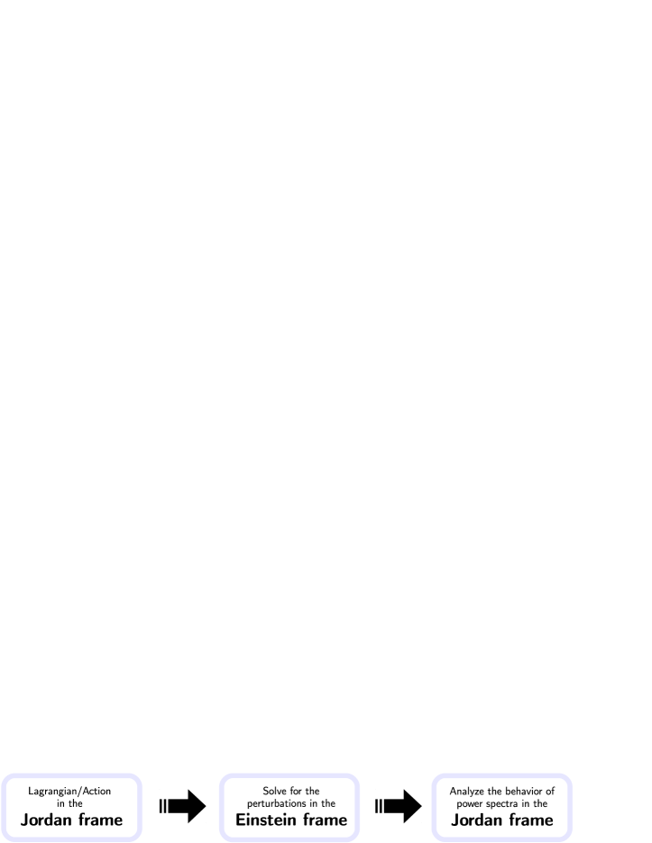
Figure 2: Flow diagram representing the procedure of regularization we followed in this work in relation to the use of the Einstein and Jordan frames.

In doing the final part, we find it extremely helpful if not crucial to do the subtraction process in the Jordan frame. In performing adiabatic regularization of the power spectrum, the knowledge of the behavior of several important parameters ($H,\epsilon$, etc.) from horizon crossing until at least the end of inflation is necessary. The information about these come in handy in the original frame. We know (or at least we can calculate them) that $\epsilon\sim 0\rightarrow 1$ during inflation and so are the behavior of $H$ and other parameters from the time corresponding to $N_{*}$, onwards.

Now suppose we consider the regularization in the Einstein frame. In order to perform the regularization in this frame, we should properly transform the parameters involved in our original model to the Einstein frame. This however, poses some problems. Based on (3.4), $\text{d}^{2}a/\text{d}t^{2}>0$ does not necessarily imply $\text{d}^{2}\widehat{a}/\text{d}\widehat{t}\,^{2}>0$; that is, inflation in the Jordan frame does not necessarily imply inflation in the Einstein frame. Furthermore, by virtue of (3.5),

$$\widehat{\epsilon} =\bigg{(}1+\frac{1}{H}\frac{\dot{\Omega}}{\Omega}\bigg{)}^{-2}\bigg{[}\epsilon+\frac{1}{H}\frac{\dot{\Omega}}{\Omega}+\frac{1}{H^{2}}\bigg{(}2\frac{\dot{\Omega}^{2}}{\Omega^{2}}-\frac{\ddot{\Omega}}{\Omega}\bigg{)}\bigg{]},$$ (5.1)

we know that $\epsilon\sim 0\rightarrow 1$ does not necessarily imply $\widehat{\epsilon}\sim 0\rightarrow 1$, nor is the average monotonically increasing behavior of $\epsilon$ crucial in establishing the exponentially decaying behavior of the Hubble parameter (see the previous section). While we know the behavior of the inflationary parameters in the Jordan frame, the same is not straightforward when we consider the transformed parameters ($H\rightarrow\widehat{H},\epsilon\rightarrow\widehat{\epsilon},N_{*}\rightarrow\widehat{N}_{*}$, etc.) in the Einstein frame. This is further complicated by the difference in the times of horizon crossing in the two frames. It is thus, far more computationally economical to do the final subtraction process in the Jordan frame where we have the original model in place.

The non-trivial mapping of inflationary parameters from the Jordan frame to the Einstein frame also tells us one important point: if the subtraction term in the regularization of the power spectrum tends to zero in the minimal case, this does not necessarily mean that the same holds in the nonminimal case. Although the result of Urakawa and Starobinsky [23] tells us that the regularization of the power spectrum in the canonical inflation yields the “bare” power spectrum, this does not necessarily mean that all corresponding nonminimally coupled inflation transformable to the canonical case through frame transformation should yield the same result. Whereas we take $\epsilon\sim 0\rightarrow\sim 1$ in the canonical case for the subtraction term, we take the same ($\epsilon\sim 0\rightarrow\sim 1$) for the nonminimal case; yet in going from the Jordan frame to the Einstein frame for the nonminimal case, we cannot simply take $\epsilon\sim 0\rightarrow\sim 1$ to $\widehat{\epsilon}\sim 0\rightarrow 1$. This is not to say that the adiabatic regularization in the Jordan and Einstein frames would yield different results. But to emphasize that at least within the framework of adiabatic regularization, the canonical case studied by Urakawa and Starobinsky [23] does not exactly correspond to the Einstein frame of the nonminimal case in this study; the behavior of the inflationary parameters may differ significantly.

With this being said, the foregoing seems to only scratch the surface of subtleties associated with frame transformation from the perspective of adiabatic regularization. It would be interesting to further explore the behavior of the subtraction term in the Einstein frame and how it relates to that in the Jordan frame. But as the nontrivial mapping between the inflationary parameters suggests computational and conceptual complexities requiring more space than we can allot here, we wish not to deviate from the main concern of this work. Looking ahead, this will be another direction along which we can extend this study.

6 Concluding Remarks

Power spectrum is one of the most important quantities in inflationary cosmology. In this work, we investigated the effect of ultraviolet (UV) regularization on the power spectrum within the framework of nonminimally coupled chaotic inflation. Our calculation suggests that the adiabatic regularization leads to no difference between the “bare” and regularized power spectra for both scalar and tensor perturbations. Going beyond the time of horizon crossing, the subtraction term exponentially decays with respect to the number of $e$-folds and becomes insignificant in the long run; the expansion of the Universe essentially erases the subtraction term. This is the same result we obtained for minimally coupled general single-field inflation in our previous study [24]. Thus, for both the minimally coupled and nonminimally coupled cases, the current and the previous studies together with that of Urakawa and Starobinsky [23], justify the use of the “bare” power spectrum in standard calculations.

So far, we have only investigated the area of nonminimally coupled inflation where the speed of sound is constant. It would be interesting to see the effect of varying speed of sound $c_{s}^{2}$, in scenarios where the usual kinetic-plus-potential term is replaced by a general “pressure” function $P(X,\phi)$, where $X\equiv-\frac{1}{2}g^{\mu\nu}\phi_{,\mu}\phi_{,\nu}$. The subtraction term would significantly be more complicated because of the involvement of the time derivatives of $c_{s}^{2}$ and the more complex relationship between the speed of sound in the Jordan and Einstein frames. From a bird’s eye view, three main terms have to be considered namely, those due to (a) the speed of sound, (b) variation of the Hubble parameter, and (c) the effects of the nonminimal coupling term. Beyond this scenario, one may also consider nonminimal inflation beyond Einstein gravity; e.g., instead of $h(\phi)R$, one may consider $h(\phi)f(R)$, where $f(R)$ is a function of the Ricci scalar. In addition to this, we have not addressed the more challenging problems involving interactions and loop corrections. Considering all these problems, we look ahead to establishing a general set of conditions within the framework of general single-field inflation, both minimal and nonminimal, that would guarantee the null effect of adiabatic regularisation on both scalar and tensor power spectra.

References

- [1] A. H. Guth, The Inflationary Universe: A Possible Solution to the Horizon and Flatness Problems, Phys. Rev. D 23 (1981) 347.
- [2] A. A. Starobinsky, A New Type of Isotropic Cosmological Models Without Singularity, Phys. Lett. B 91 (1980) 99. doi:10.1016/0370-2693(80)90670-X
- [3] A. A. Starobinsky, Spectrum of relict gravitational radiation and the early state of the universe, JETP Lett. 30 (1979) 682 [Pisma Zh. Eksp. Teor. Fiz. 30 (1979) 719].
- [4] K. Sato, First Order Phase Transition of a Vacuum and Expansion of the Universe, Mon. Not. Roy. Astron. Soc. 195 (1981) 467.
- [5] A. D. Linde, Chaotic Inflation, Phys. Lett. B 129 (1983) 177. doi:10.1016/0370-2693(83)90837-7
- [6] A. Albrecht and P. J. Steinhardt, Cosmology for Grand Unified Theories with Radiatively Induced Symmetry Breaking, Phys. Rev. Lett. 48 (1982) 1220. doi:10.1103/PhysRevLett.48.1220
- [7] A. R. Liddle, D. H. Lyth, The primordial density perturbation: Cosmology, inflation and the origin of structure, NY, USA: Cambridge Univ. Pr. (2009) 516 p.
- [8] V. Mukhanov, Physical Foundations of Cosmology, NY, USA: Cambridge Univ. Pr. (2005) 421 p.
- [9] P. A. R. Ade et al. [Planck Collaboration], Planck 2013 results. XXII. Constraints on inflation, Astron. Astrophys. 571 (2014) A22 doi:10.1051/0004-6361/201321569 [arXiv:1303.5082 [astro-ph.CO]].
- [10] P. A. R. Ade et al. [Planck Collaboration], Planck 2015 results. XX. Constraints on inflation, arXiv:1502.02114 [astro-ph.CO].
- [11] L. Senatore and M. Zaldarriaga, On Loops in Inflation, JHEP 1012 (2010) 008 doi:10.1007/JHEP12(2010)008 [arXiv:0912.2734 [hep-th]].
- [12] D. Seery, One-loop corrections to a scalar field during inflation, JCAP 0711 (2007) 025 doi:10.1088/1475-7516/2007/11/025 [arXiv:0707.3377 [astro-ph]].
- [13] L. Parker, D. J. Toms Quantum Field Theory in Curved Spacetime, Cambridge, UK: Univ. Pr. (2009) 472 p.
- [14] A. Contillo, M. Hindmarsh and C. Rahmede, Renormalisation group improvement of scalar field inflation, Phys. Rev. D 85 (2012) 043501 doi:10.1103/PhysRevD.85.043501 [arXiv:1108.0422 [gr-qc]].
- [15] L. Parker and S. A. Fulling, Adiabatic regularization of the energy momentum tensor of a quantized field in homogeneous spaces, Phys. Rev. D 9 (1974) 341 .
- [16] S. A. Fulling, L. Parker and B. L. Hu, Conformal energy-momentum tensor in curved spacetime: Adiabatic regularization and renormalization, Phys. Rev. D 10 (1974) 3905 .
- [17] T. S. Bunch, Adiabatic Regularization For Scalar Fields With Arbitrary Coupling To The Scalar Curvature, J. Phys. A 13 (1980) 1297.
- [18] R. Fakir and W. G. Unruh, Improvement on cosmological chaotic inflation through nonminimal coupling, Phys. Rev. D 41 (1990) 1783. doi:10.1103/PhysRevD.41.1783
- [19] T. Futamase and K. Maeda, Chaotic Inflationary Scenario in Models Having Nonminimal Coupling With Curvature, Phys. Rev. D 39 (1989) 399. doi:10.1103/PhysRevD.39.399
- [20] N. Makino and M. Sasaki, The Density perturbation in the chaotic inflation with nonminimal coupling, Prog. Theor. Phys. 86 (1991) 103. doi:10.1143/PTP.86.103
- [21] E. Komatsu and T. Futamase, Complete constraints on a nonminimally coupled chaotic inflationary scenario from the cosmic microwave background, Phys. Rev. D 59 (1999) 064029 doi:10.1103/PhysRevD.59.064029 [astro-ph/9901127].
- [22] K. Nozari and S. Shafizadeh, Non-Minimal Inflation Revisited, Phys. Scripta 82 (2010) 015901 doi:10.1088/0031-8949/82/01/015901 [arXiv:1006.1027 [gr-qc]].
- [23] Y. Urakawa and A. A. Starobinsky, Adiabatic regularization of primordial perturbations generated during inflation, Proc. 19th Workshop in General Relativity and Gravitation in Japan (JGRG19), Tokyo, Japan, pp. 367-371 [http://www2.rikkyo.ac.jp/web/jgrg19/Proceedings/pdf/O25.pdf].
- [24] A. L. Alinea, T. Kubota, Y. Nakanishi and W. Naylor, Adiabatic regularisation of power spectra in -inflation, JCAP 1506 (2015) no.06, 019 doi:10.1088/1475-7516/2015/06/019 [arXiv:1503.08073 [gr-qc]].
- [25] J. M. Bardeen, Gauge Invariant Cosmological Perturbations, Phys. Rev. D 22 (1980) 1882. doi:10.1103/PhysRevD.22.1882
- [26] N. D. Birrell and P. C. W. Davies, Quantum Fields in curved space, Cambridge, Great Britain: Press Syndicate of the University of Cambridge (1982) 352 p.
- [27] L. Parker, Amplitude of Perturbations from Inflation, hep-th/0702216 [HEP-TH].
- [28] I. Agullo, J. Navarro-Salas, G. J. Olmo and L. Parker, Revising the predictions of inflation for the cosmic microwave background anisotropies, Phys. Rev. Lett. 103 (2009) 061301 [arXiv:0901.0439 [astro-ph.CO]].
- [29] I. Agullo, J. Navarro-Salas, G. J. Olmo and L. Parker, Revising the observable consequences of slow-roll inflation, Phys. Rev. D 81 (2010) 043514 [arXiv:0911.0961 [hep-th]].
- [30] F. Finelli, G. Marozzi, G. P. Vacca and G. Venturi, The Impact of ultraviolet regularization on the spectrum of curvature perturbations during inflation, Phys. Rev. D 76 (2007) 103528 [arXiv:0707.1416 [hep-th]].
- [31] R. Durrer, G. Marozzi and M. Rinaldi, On Adiabatic Renormalization of Inflationary Perturbations, Phys. Rev. D 80 (2009) 065024 [arXiv:0906.4772 [astro-ph.CO]].
- [32] M. Bastero-Gil, A. Berera, N. Mahajan and R. Rangarajan, Power spectrum generated during inflation, Phys. Rev. D 87 (2013) 8, 087302 [arXiv:1302.2995 [astro-ph.CO]].
- [33] A. Linde, M. Noorbala and A. Westphal, Observational consequences of chaotic inflation with nonminimal coupling to gravity, JCAP 1103 (2011) 013 doi:10.1088/1475-7516/2011/03/013 [arXiv:1101.2652 [hep-th]].
- [34] M. P. Hertzberg, On Inflation with Non-minimal Coupling, JHEP 1011 (2010) 023 doi:10.1007/JHEP11(2010)023 [arXiv:1002.2995 [hep-ph]].
- [35] T. Inagaki, R. Nakanishi and S. D. Odintsov, Non-Minimal Two-Loop Inflation, Phys. Lett. B 745 (2015) 105 doi:10.1016/j.physletb.2015.04.038 [arXiv:1502.06301 [hep-ph]].
- [36] T. Qiu and K.-C. Yang, Non-Gaussianities of single field inflation with nonminimal coupling, Phys. Rev. D 83 (2011) 084022 [arXiv:1012.1697 [hep-th]].
- [37] E. Elizalde, S. D. Odintsov, E. O. Pozdeeva and S. Y. Vernov, Cosmological attractor inflation from the RG-improved Higgs sector of finite gauge theory, JCAP 1602 (2016) no.02, 025 doi:10.1088/1475-7516/2016/02/025 [arXiv:1509.08817 [gr-qc]].
- [38] R. L. Arnowitt, S. Deser and C. W. Misner, Dynamical Structure and Definition of Energy in General Relativity, Phys. Rev. 116, (1959) 1322.
- [39] E. Gourgoulhon, 3 + 1 Formalism in General Relativity, Berlin, Germany: Springer (2012) 294 p.
- [40] X. Chen, Primordial Non-Gaussianities from Inflation Models, Adv. Astron. 2010 (2010) 638979 doi:10.1155/2010/638979 [arXiv:1002.1416 [astro-ph.CO]].
- [41] T. Kubota, N. Misumi, W. Naylor and N. Okuda, The Conformal Transformation in General Single Field Inflation with Non-Minimal Coupling, JCAP 1202 (2012) 034 [arXiv:1112.5233 [gr-qc]].
- [42] T. Zhu, A. Wang, G. Cleaver, K. Kirsten and Q. Sheng, Power spectra and spectral indices of -inflation: high-order corrections, Phys. Rev. D 90 (2014) no.10, 103517 doi:10.1103/PhysRevD.90.103517 [arXiv:1407.8011 [astro-ph.CO]].
- [43] J. Martin, C. Ringeval and V. Vennin, K-inflationary Power Spectra at Second Order, JCAP 1306 (2013) 021 doi:10.1088/1475-7516/2013/06/021 [arXiv:1303.2120 [astro-ph.CO]].
- [44] S. Habib, K. Heitmann, G. Jungman and C. Molina-Paris, The Inflationary perturbation spectrum, Phys. Rev. Lett. 89 (2002) 281301 doi:10.1103/PhysRevLett.89.281301 [astro-ph/0208443].
- [45] S. Habib, A. Heinen, K. Heitmann, G. Jungman and C. Molina-Paris, Characterizing inflationary perturbations: The Uniform approximation, Phys. Rev. D 70 (2004) 083507 doi:10.1103/PhysRevD.70.083507 [astro-ph/0406134].
- [46] A. L. Alinea, T. Kubota and W. Naylor, Logarithmic divergences in the -inflationary power spectra computed through the uniform approximation, JCAP 1602 (2016) no.02, 028 doi:10.1088/1475-7516/2016/02/028 [arXiv:1506.08344 [gr-qc]].
- [47] J. O. Gong and E. D. Stewart, The Density perturbation power spectrum to second order corrections in the slow roll expansion, Phys. Lett. B 510 (2001) 1 doi:10.1016/S0370-2693(01)00616-5 [astro-ph/0101225].
- [48] J. Martin and D. J. Schwarz, WKB approximation for inflationary cosmological perturbations, Phys. Rev. D 67 (2003) 083512 doi:10.1103/PhysRevD.67.083512 [astro-ph/0210090].
- [49] R. Casadio, F. Finelli, M. Luzzi and G. Venturi, Improved WKB analysis of slow-roll inflation, Phys. Rev. D 72 (2005) 103516 doi:10.1103/PhysRevD.72.103516 [gr-qc/0510103].
- [50] D. J. Schwarz, C. A. Terrero-Escalante and A. A. Garcia, Higher order corrections to primordial spectra from cosmological inflation, Phys. Lett. B 517 (2001) 243 doi:10.1016/S0370-2693(01)01036-X [astro-ph/0106020].
- [51] K. Nozari and N. Rashidi, Testing an Inflation Model with Nonminimal Derivative Coupling in the Light of PLANCK 2015 Data, Adv. High Energy Phys. 2016 (2016) 1252689 doi:10.1155/2016/1252689 [arXiv:1509.06240 [astro-ph.CO]].
- [52] A. Salvio and A. Mazumdar, Classical and Quantum Initial Conditions for Higgs Inflation, Phys. Lett. B 750 (2015) 194 doi:10.1016/j.physletb.2015.09.020 [arXiv:1506.07520 [hep-ph]].
- [53] V. Faraoni and S. Nadeau, The (pseudo)issue of the conformal frame revisited, Phys. Rev. D 75 (2007) 023501 doi:10.1103/PhysRevD.75.023501 [gr-qc/0612075].
- [54] V. Faraoni and E. Gunzig, Einstein frame or Jordan frame?, Int. J. Theor. Phys. 38 (1999) 217 doi:10.1023/A:1026645510351 [astro-ph/9910176].