A nonequilibrium diffusion and capture mechanism ensures tip-localization of regulating proteins on dynamic filaments
Abstract
Diffusive motion of regulatory enzymes on biopolymers with eventual capture at a reaction site is a common feature in cell biology. Using a lattice gas model we study the impact of diffusion and capture for a microtubule polymerase and a depolymerase. Our results show that the capture mechanism localizes the proteins and creates large-scale spatial correlations. We develop an analytic approximation that globally accounts for relevant correlations and yields results that are in excellent agreement with experimental data. Our results show that diffusion and capture operates most efficiently at cellular enzyme concentrations which points to in vivo relevance.
The diffusive motion of proteins on filamentous structures in the cell is vital for several cellular functions such as gene regulation Hippel1989 and cytoskeletal dynamics Cooper2009; Howard2007: To find their target sites, transcription factors are likely to employ one-dimensional diffusion on the DNA and the dynamics of this process largely determine the kinetics of gene regulation Riggs1970; Hammar2012. Similarly, actin and microtubule (MT) binding proteins diffuse on the respective filaments and fulfill regulatory functions primarily at the filament ends. Adam and Delbrück Adam1968 suggested that a reduction in dimensionality of the diffusive motion enhances the effective rate of association of particles with binding sites on the membrane or on DNA and filaments, and this concept has been widely applied and extended Richter1974; *Berg1981; Bintu2005, see also Refs. Mirny2009; *Kolomeisky2011; *Benichou2011; *Sheinman2012 for recent reviews on the topic.
With regard to cytoskeletal architectures, efficient association and localization of enzymes to specific sites is relevant for a variety of cellular processes throughout the cell cycle and for cell motility and dynamics Dos2003; *Akhmanova2008. It was recently shown experimentally that one-dimensional diffusion is utilized Helenius2006; Cooper2009 by two proteins with important roles in the regulation of MT dynamics Tournebize2000; Kinoshita2001; Wilbur2013; Reber2013, MCAK and XMAP215. These proteins strongly localize at their respective reaction sites and show association rates for these sites that are significantly higher than expected for binding via three-dimensional diffusion Helenius2006; Brouhard2008. Both proteins carry out vital tasks, with MCAK acting as depolymerase of tubulin protofilaments Desai1999 and XMAP215 as a poylmerase Brouhard2008 when bound to ends of MTs. Note that similar mechanisms are also assumed to be relevant for actin associated proteins Romero2004; *Vavylonis2006; *Hansen2010; *Mizuno2011. However, diffusive motion on filaments does not lead to a localization and efficient association of proteins per se: As we have shown previously Reithmann2015, it is crucial to include a capturing mechanism at the reaction site, which suppresses the one-dimensional diffusive motion of a protein that reaches this site; without such a capturing mechanism no increase in the effective association rate for the tip occurs. For MCAK and XMAP215 protein capturing is observed in experiments: Diffusive motion stops once the proteins reach the MT tip Brouhard2008; Helenius2006. Yet, the underlying interactions with the MT tip are still elusive and being studied Friel2011; *Ritter2016.
Here we present a theoretical description of enzyme diffusion and capture at MT tips where the enzymes catalyze filament polymerization or depolymerization. Previous studies of similar systems have lacked either a capturing mechanism Klein2005; Schmitt2011 or a dynamic filament Reithmann2015, although both features are critical. To overcome both limitations, we employ a one-dimensional lattice gas Chou2011; Derrida1998 with particle capturing in a dynamic system, in which growth or shrinkage of the filament is triggered by the interactions of particles with the lattice end. Our motivation is twofold: Firstly, we seek for a detailed mathematical understanding of the capturing mechanism. Secondly, based on a fully quantitative model, we wish to elucidate the specific biomolecular mechanisms employed by XMAP215 and MCAK. Our results show that the capturing process induces large-scale spatial correlations in the protein distribution along the filament. We develop a mathematical framework that systematically includes relevant correlations on a global scale. This conceptual advancement allows us to quantitatively explain the results of in vitro experiments with XMAP215 and MCAK Brouhard2008; Cooper2010. We demonstrate that the diffusion and capture mechanism strongly localizes XMAP215 and MCAK at the MT tip and that the process operates optimally under physiological conditions for both proteins, which suggests that it is relevant in vivo.

Model definition.
We consider a one-dimensional lattice with lattice spacing and a semi-infinite geometry which corresponds to one protofilament, as depicted in Fig. 1. In the case of MTs, is the length of a tubulin heterodimer, . The configuration of enzymes on the lattice is described by occupation numbers , taking values for empty, and for occupied sites. The particles symmetrically hop to neighboring sites at rate , and interact via hard-core repulsion. We implement Langmuir kinetics to model a surrounding reservoir of particles with a constant concentration . Particles attach to and detach from the lattice at rates and , respectively Lipowsky2001; Parmeggiani2003; *Parmeggiani2004. Sites are considered as bulk sites. There the dynamics differs from that in the bulk as we implement a protein capturing mechanism: Hopping from site to site is disallowed, as suggested experimentally for MCAK and XMAP215 Helenius2006; Brouhard2008. In this way, detailed balance is broken which leads to strong tip-localization due to a particle flux along the filament; in equilibrium models such a significant localization is absent, see Fig. S1 in the Supporting Material SuppMat. Particles detach from the first lattice site at a distinct off-rate, . We refer to site as a reaction site at which new lattice sites may be added or removed. For the moment, we specify our discussion to polymerases such as XMAP215 Brouhard2008. However, our considerations are largely independent of whether polymerization or depolymerization occurs—an equivalent formulation can also be found for the depolymerase MCAK SuppMat. For XMAP215, we specify that lattice growth is triggered at rate if the protein is bound to the first lattice site. Hence, the average speed of lattice growth for the MT is proportional to the average particle occupation and the XMAP215 polymerization rate: . Here we assume one catalyzing protein per protofilament end at saturating conditions SuppMat. The actual maximum number of catalytically active proteins is unknown; in experimental literature approximately 10 XMAP215 proteins at the MT tip are estimated at XMAP215 Brouhard2008. As shown in recent experiments, XMAP215 acts processively, i.e. one molecule adds multiple tubulin dimers to the growing MT end Brouhard2008. To implement such behavior in our model the particle at the tip is transferred to newly incorporated lattice sites. In our analysis we neglect uncatalyzed tubulin addition or removal as typical corresponding experiments Helenius2006; Cooper2010; Brouhard2008; Widlund2011 were performed under conditions where these processes did not occur with a significant rate. An extension is, however, possible in a straightforward fashion and does not affect tip-localization significantly; see Fig. S5 and S6 in the Supporting Material SuppMat. Therefore we expect validity of our further considerations also with intrinsic MT dynamics, for example as a consequence of hydrolysis of tubulin bound GTP which was studied extensively in previous models Antal2007; *Padinhateeri2012; *Niedermayer2015.
Mathematical analysis.
We set up the equations of motion for the average occupation numbers of the stochastic process defined above. All equations will be formulated in the frame of reference comoving with the dynamic lattice end. In the bulk of the lattice, , we obtain
| (1) | |||||
This equation comprises contributions from hopping while obeying the exclusion principle Derrida2007 (terms proportional to ) and a displacement current due to polymerization (terms proportional to ) as well as particle attachment and detachment (terms proportional to and , respectively). The tip occupations complement these bulk dynamics in the following manner:
| (2) | |||||
Here we have defined the average density, , and the correlation function, . Moreover, since the polymerization process facilitated by XMAP215 is processive, an empty lattice site at is created and site remains occupied each time a new site is added. We fully quantify our model with the experimental data available for XMAP215 Brouhard2008; Widlund2011; see Supporting Material for parameter values SuppMat.
In the first step we test the quality of standard approximation techniques for driven lattice gases against stochastic simulation data obtained from Gillespie’s algorithm Gillespie2007. The set of equations which determines the lattice occupations (Eq. 1 and Eqs. 2) is not closed; the dynamics of the density and the correlation functions are coupled. In fact, there is a hierarchy of equations, which, in general, precludes the derivation of an exact solution for many driven lattice gas systems. A common and often quite successful approximation scheme for exclusion processes is to assume that there are no correlations and that one may factorize all correlation functions, . In this mean-field (MF) approximation one obtains a closed set of differential equations for the particle density which may be solved subject to proper boundary conditions; see Supporting Material for details. Fig. 2 shows the average occupation number of the first site, , as a function of the protein concentration in solution . A comparison with our stochastic simulation data shows that the MF solution strongly overestimates and thus the average polymerization speed .
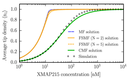
One possible reason for the failure of the MF calculation lies in correlations that arise close to the reaction site. Local correlations can efficiently be accounted for by employing a finite segment mean-field (FSMF) theory Chou2004; Lakatos2005. Here, the idea is to retain all correlations close to the catalytic site by solving the full master equation for the first sites and to use the MF assumption only outside of this segment. The density profile is then obtained by matching the tip solution and the MF solution Klein2005; Nowak2007; see Supporting Material SuppMat. While the results show the right trend towards the numerical data, the improvement over the MF results is insignificant. These observations suggest that correlations extend far beyond the immediate vicinity of the reaction site.
To account for such correlations we extend the MF theory by retaining both the density and the correlation function as dynamic variables. In order to close the set of equations we employ the following factorization scheme: , and for , i.e. we retain correlations with respect to the reaction site but neglect them within the bulk of the lattice. We confirmed this approximation scheme for typical biological parameter values by stochastic simulations; see Fig. S2 in the Supporting Material SuppMat. With the above closure relations one obtains for the bulk dynamics in a continuous description
| (3a) | |||||
| (3b) | |||||
where we defined and with for . We have further introduced the macroscopic diffusion constant and the maximum polymerization speed . Equations 3 can be derived from the discrete equations for the density , Eq. 1, and the correlation function ; for details see the Supporting Material SuppMat. Due to the capturing mechanism a continuous description is not valid at sites , and we retain the local dynamics there, Eqs. 2. These equations constrain the boundary conditions of and at . We further impose that the density equilibrates asymptotically at the Langmuir isotherm, , and that correlations vanish, . Solving the equations of this correlated MF (CMF) theory for the steady state tip density we obtain the results shown in Fig. 2, which are in excellent agreement with the stochastic simulation data. We therefore conclude that there are long-ranged correlations along the MT and that they are essential in explaining the observed average tip density and the ensuing polymerization speed.
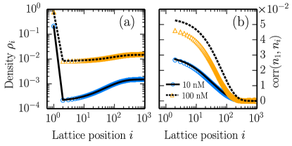
Fig. 3(a) shows the density profile along the lattice obtained by stochastic simulations and the CMF approach. The particle occupation is obtained with high precision within the CMF framework along the whole lattice. The density profiles also agree with recent data from time and ensemble averaged high resolution fluorescence intensity profiles for XMAP215 Maurer2014. Notably, there is a discontinuity at sites , which is due to particle capture and which demonstrates the strong tip-localization of the proteins.
In Figure 3(b), the Pearson product-momentum correlation coefficient
| (4) |
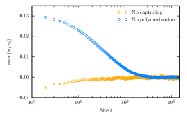
which quantifies the correlations between the tip site and sites in the bulk, is plotted against lattice position. Here , and signify the covariance and the standard deviation, respectively. The correlation coefficient decays very slowly over a broad region at the tip. The capturing mechanism and the resulting particle flux towards the filament tip ensue strong positive correlations with respect to the first lattice site and sites in its vicinity. This effect is antagonized by weak negative correlations caused by the creation of empty lattice sites due to polymerization. With diffusion taking place on a faster time scale than polymerization, the positive correlations dominate. This is confirmed by stochastic simulations where either capturing or growth is switched off: We find anti-correlations if capturing is turned off, and positive correlations if there is no growth of the lattice; see Fig. S3 in the Supporting Material SuppMat. Note that for higher growth rates the correlation profile can also become negative. We conclude that the spatial correlations which emerge over several hundred lattice sites are a direct consequence of protein capture and processive growth. Further, it becomes evident why the MF and the FSMF approaches do not lead to the correct tip density: Correlations extend into the system on a length-scale which exceeds the scope of these and other previous approaches Schmitt2011; Klein2005; Reithmann2015. In contrast the CMF approximation captures and quantifies significant correlations and successfully reproduces simulation data. Note that also higher order correlations of the form and with and , which are neglected in the CMF approximation, might be of relevance when particle interactions become important for lattice diffusion. This explains the deviations in the computed correlation profile, Fig 3(b). As the CMF method is based on a non-perturbative ansatz there is no analytic expression that exactly quantifies its error. However, we observe very good agreement with our Gillespie algorithm based simulations over a very broad parameter range and, importantly, for typical biological parameters, see Fig. S4 in the Supporting Material SuppMat.
Comparison with experimental data.
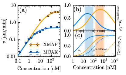
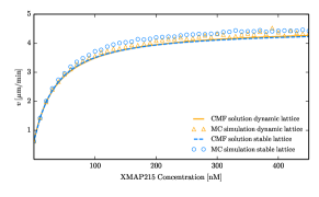
We now turn to a comparison with experimental data for the polymerization velocity Brouhard2008; Widlund2011 and, to supplement the results for XMAP215, we apply our methods to an analogous model for MCAK particles which depolymerize MTs Helenius2006; Cooper2010. In essence, we adapt the above model to account for lattice shrinkage triggered by an occupied reaction site, see Supporting Material for details SuppMat. Similar to the processive polymerization of XMAP215 also MCAK is assumed to depolymerize processively Helenius2006; Cooper2010. The parameters employed in the model are again drawn from available experimental data Cooper2010. For both MCAK and XMAP215, we find excellent quantitative agreement between our theoretical approach and experimentally determined polymerization and depolymerization velocities; see Fig. 4(a). This quantitative agreement is achieved without an adjustable parameter; see Supporting Material SuppMat. We then used the quantified models to investigate the impact of the diffusion and capture process for XMAP215 and MCAK. Fig. 4(b) shows the increase of protein localization at the reaction site due to diffusion and capture on the filament: We plot the difference between tip densities in the presence () and absence of diffusion on filaments (). For both enzymes, diffusive motion and subsequent capturing at the MT lattice strongly increases the occupation density at the tip and therefore constitutes a highly efficient means of increasing the effective attachment rate to the reaction site. Moreover, the ensuing curve shows a pronounced maximum, indicating an optimal concentration range at which the enhancement of tip occupancy due to diffusion on the MT reaches its peak. Strikingly, this maximum coincides with the physiological concentration range for each protein: for XMAP215 Kinoshita2001 and Hunter2003 for MCAK. This strongly supports the importance of diffusion and capture for MCAK and XMAP215 in vivo.
It is interesting to speculate about possible biomolecular mechanisms that could generate particle capturing at the MT tip as such a mechanism would probably require an energy source to drive the system out of equilibrium. Concerning MCAK, it was recently hypothesized, that an ATP is required to stop its diffusive motion at the MT tip Friel2011; Ritter2016 which is consistent with our proposed non-equilibrium model. Since XMAP215 does not bind nucleotides such as ATP or GTP itself Brouhard2008, one might speculate that a non-equilibrium capturing mechanism relies on tubulin polymerization or depolymerization. Possibly, a conformational change of XMAP215 coupled to processes involved in MT depolymerization or polymerization could lead to protein capture.
Summary and Conclusion.
In this work, we studied the regulatory influence of an explicit capture process on the distribution of MT polymerases and depolymerases that are subject to one-dimensional diffusion on MTs. To model these biologically relevant situations we employed a model based on a symmetric simple exclusion process Derrida1998 extended by a detailed balance breaking capturing process at the lattice end, which acts as a biasing mechanism. Our results show that the occupation of the MT tip with a protein spatially correlates with the occupation of the MT lattice. This is a direct consequence of protein capturing which in turn strongly localizes the proteins at the MT tip. Correlations decay slowly along the lattice and have a large impact on the occupation of the MT tip. This is of relevance as the latter quantity determines the velocity of enzyme-dependent MT growth or shrinking. We derive a generalized set of hydrodynamic equations which couple the evolution of the particle density with the evolution of relevant correlations. In that way it is possible to account for those correlations on a global scale. Similar correlations have been identified in two-dimensional diffusive systems Markham2013a; *Markham2013b or in diffusive systems with a small, local drive Sadhu2014.
Our findings are not limited to MTs and their associated enzymes, but might also be applicable to other enzymatic processes with spatial degrees of freedom and, quite generally, non-equilibrium physics.
Acknowledgements.
We thank Linda Wordeman, Gary Brouhard and their respective co-workers for sharing data points of XMAP215 and MCAK induced MT growing and shrinking velocities, respectively, as shown in Fig. 4(a). This research was supported by the German Excellence Initiative via the program “NanoSystems Initiative Munich” (NIM) and the Deutsche Forschungsgemeinschaft (DFG) via project B02 within the Collaborative Research Center (SFB 863) “Forces in Biomolecular Systems”.References
- von Hippel and Berg (1989) P. H. von Hippel and O. G. Berg, J. Biol. Chem. 264, 675 (1989).
- Cooper and Wordeman (2009) J. R. Cooper and L. Wordeman, Curr. Opin. Cell Biol. 21, 68 (2009).
- Howard and Hyman (2007) J. Howard and A. A. Hyman, Curr. Opin. Cell Biol. 19, 31 (2007).
- Riggs et al. (1970) A. D. Riggs, H. Suzuki, and S. Bourgeois, J. Mol. Biol. 48, 67 (1970).
- Hammar et al. (2012) P. Hammar, P. Leroy, A. Mahmutovic, E. G. Marklund, O. G. Berg, and J. Elf, Science 336, 1595 (2012).
- Adam and Delbrück (1968) G. Adam and M. Delbrück, in Structural chemistry and molecular biology (Freeman, 1968) pp. 198–215.
- Richter and Eigen (1974) P. H. Richter and M. Eigen, Biophys. Chem. 2, 255 (1974).
- Berg et al. (1981) O. G. Berg, R. B. Winter, and P. H. Von Hippel, Biochemistry 20, 6929 (1981).
- Bintu et al. (2005) L. Bintu, N. E. Buchler, H. G. Garcia, U. Gerland, T. Hwa, J. Kondev, and R. Phillips, Curr. Opin. Genet. Dev. 15, 116 (2005).
- Mirny et al. (2009) L. Mirny, M. Slutsky, Z. Wunderlich, A. Tafvizi, J. Leith, and A. Kosmrlj, J. Phys. A: Math. Theor. 42, 434013 (2009).
- Kolomeisky (2011) A. B. Kolomeisky, Phys. Chem. Chem. Phys. 13, 2088 (2011).
- Bénichou et al. (2011) O. Bénichou, C. Loverdo, M. Moreau, and R. Voituriez, Rev. Mod. Phys. 83, 81 (2011).
- Sheinman et al. (2012) M. Sheinman, O. Bénichou, Y. Kafri, and R. Voituriez, Rep. Prog. Phys. 75, 026601 (2012).
- Dos Remedios et al. (2003) C. G. Dos Remedios, D. Chhabra, M. Kekic, I. V. Dedova, M. Tsubakihara, D. A. Berry, and N. J. Nosworthy, Physiol. Rev. 83, 433 (2003).
- Akhmanova and Steinmetz (2008) A. Akhmanova and M. O. Steinmetz, Nat. Rev. Mol. Cell Biol. 9, 309 (2008).
- Helenius et al. (2006) J. Helenius, G. J. Brouhard, Y. Kalaidzidis, S. Diez, and J. Howard, Nature 441, 115 (2006).
- Tournebize et al. (2000) R. Tournebize, A. Popov, K. Kinoshita, A. J. Ashford, S. Rybina, A. Pozniakovsky, T. U. Mayer, C. E. Walczak, E. Karsenti, and A. A. Hyman, Nat. Cell Biol. 2, 13 (2000).
- Kinoshita et al. (2001) K. Kinoshita, I. Arnal, A. Desai, D. N. Drechsel, and A. A. Hyman, Science 294, 1340 (2001).
- Wilbur and Heald (2013) J. D. Wilbur and R. Heald, eLife 2, e00290 (2013).
- Reber et al. (2013) S. B. Reber, J. Baumgart, P. O. Widlund, A. Pozniakovsky, J. Howard, A. A. Hyman, and F. Jülicher, Nat. Cell Biol. 15, 1116 (2013).
- Brouhard et al. (2008) G. J. Brouhard, J. H. Stear, T. L. Noetzel, J. Al-Bassam, K. Kinoshita, S. C. Harrison, J. Howard, and A. A. Hyman, Cell 132, 79 (2008).
- Desai et al. (1999) A. Desai, S. Verma, T. J. Mitchison, and C. E. Walczak, Cell 96, 69 (1999).
- Romero et al. (2004) S. Romero, C. Le Clainche, D. Didry, C. Egile, D. Pantaloni, and M.-F. Carlier, Cell 119, 419 (2004).
- Vavylonis et al. (2006) D. Vavylonis, D. R. Kovar, B. O’Shaughnessy, and T. D. Pollard, Mol. Cell 21, 455 (2006).
- Hansen and Mullins (2010) S. D. Hansen and R. D. Mullins, J. Cell Biol. 191, 571 (2010).
- Mizuno et al. (2011) H. Mizuno, C. Higashida, Y. Yuan, T. Ishizaki, S. Narumiya, and N. Watanabe, Science 331, 80 (2011).
- Reithmann et al. (2015) E. Reithmann, L. Reese, and E. Frey, Biophys. J. 108, 787 (2015).
- Friel and Howard (2011) C. T. Friel and J. Howard, EMBO J. 30, 3928 (2011).
- Ritter et al. (2016) A. Ritter, N. Kreis, F. Louwen, L. Wordeman, and J. Yuan, Crit. Rev. Biochem. Mol. Bio. 51, 228 (2016).
- Klein et al. (2005) G. Klein, K. Kruse, G. Cuniberti, and F. Jülicher, Phys. Rev. Lett. 94, 108102 (2005).
- Schmitt and Stark (2011) M. Schmitt and H. Stark, Europhys. Lett. 96, 28001 (2011).
- Chou et al. (2011) T. Chou, K. Mallick, and R. K. P. Zia, Rep. Prog. Phys. 74, 116601 (2011).
- Derrida (1998) B. Derrida, Phys. Rep. 301, 65 (1998).
- Cooper et al. (2010) J. R. Cooper, M. Wagenbach, C. L. Asbury, and L. Wordeman, Nat. Struct. Mol. Biol. 17, 77 (2010).
- (35) See Supplemental Material.
- Lipowsky et al. (2001) R. Lipowsky, S. Klumpp, and T. Nieuwenhuizen, Phys. Rev. Lett. 87, 108101 (2001).
- Parmeggiani et al. (2003) A. Parmeggiani, T. Franosch, and E. Frey, Phys. Rev. Lett. 90, 86601 (2003).
- Parmeggiani et al. (2004) A. Parmeggiani, T. Franosch, and E. Frey, Phys. Rev. E 70, 46101 (2004).
- Widlund et al. (2011) P. O. Widlund, J. H. Stear, A. Pozniakovsky, M. Zanic, S. Reber, G. J. Brouhard, A. A. Hyman, and J. Howard, Proc. Nat. Acad. Sci. USA 108, 2741 (2011).
- Antal et al. (2007) T. Antal, P. L. Krapivsky, S. Redner, M. Mailman, and B. Chakraborty, Phys. Rev. E 76, 041907 (2007).
- Padinhateeri et al. (2012) R. Padinhateeri, A. B. Kolomeisky, and D. Lacoste, Biophys. J. 102, 1274 (2012).
- Niedermayer and Lipowsky (2015) T. Niedermayer and R. Lipowsky, Phys. Rev. E 92, 052137 (2015).
- Derrida (2007) B. Derrida, J. Stat. Mech. Theor. Exp. 2007, P07023 (2007).
- Gillespie (2007) D. T. Gillespie, Annu. Rev. Phys. Chem. 58, 35 (2007).
- Chou and Lakatos (2004) T. Chou and G. Lakatos, Phys. Rev. Lett. 93, 198101 (2004).
- Lakatos et al. (2005) G. Lakatos, T. Chou, and A. Kolomeisky, Phys. Rev. E 71, 011103 (2005).
- Nowak et al. (2007) S. Nowak, P.-W. Fok, and T. Chou, Phys. Rev. E 76, 31135 (2007).
- Maurer et al. (2014) S. P. Maurer, N. I. Cade, G. Bohner, N. Gustafsson, E. Boutant, and T. Surrey, Curr. Biol. 24, 372 (2014).
- Hunter et al. (2003) A. W. Hunter, M. Caplow, D. L. Coy, W. O. Hancock, S. Diez, L. Wordeman, and J. Howard, Mol. Cell 11, 445 (2003).
- Markham et al. (2013a) D. C. Markham, M. J. Simpson, and R. E. Baker, Phys. Rev. E 87, 062702 (2013a).
- Markham et al. (2013b) D. C. Markham, M. J. Simpson, P. K. Maini, E. A. Gaffney, and R. E. Baker, Phys. Rev. E 88, 052713 (2013b).
- Sadhu et al. (2014) T. Sadhu, S. N. Majumdar, and D. Mukamel, Phys. Rev. E 90, 012109 (2014).
Supplemental Material: A nonequilibrium diffusion and capture mechanism ensures tip-localization of regulating proteins on dynamic filaments
Emanuel Reithmann, Louis Reese, and Erwin Frey
Arnold Sommerfeld Center for Theoretical Physics (ASC) and Center for NanoScience (CeNS), Department of Physics, Ludwig-Maximilians-Universität München, Theresienstrasse 37, 80333 München, Germany
I Tip localization due to particle capturing
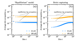
In this work, we investigate a model where the diffusive motion of particles on a filament ceases as soon as they arrive at a reaction site. This feature, which we refer to as particle capturing, is a key element of our model, as it drives the system out of thermal equilibrium. In order to investigate the impact of particle capture on tip localization of particles, we also investigated a model where particles are not captured at the tip, but where a hopping from the tip into the bulk occurs such that detailed balance is not broken. In detail, we introduce a release rate , at which particles hop from site to site . Then, to implement equilibrium conditions for particle hopping (i.e. with respect to a system without lattice growth or shrinkage), we impose . This condition ensures detailed balance in a static system and for a constant on-rate along the lattice. Since we also implement lattice growth, detailed balance is still broken, which manifests itself in a net particle drift away from the tip in the comoving frame of reference. In Fig. S1 we compare density profiles of the hopping-equilibrium model and the one with strict (i.e. irreversible) particle capturing as defined in the main text with parameters as for XMAP215. In the equilibrium model, the density profile is almost constant whereas in the model with capturing a strong tip-localization occurs (1-2 orders of magnitude increase in the tip-density). Although an irreversible capturing is, of course, a simplification, we expect similar effects to occur for release rates much smaller than the equilibrium release rate, . In this case, capturing generates a particle current towards the MT tip which conversely leads to spatial correlations subject of this work.
II Mean-field (MF) approximation
In the mean-field approximation all correlations are neglected; we set . This closes the hierarchy of equations stated in the main text:
| (S1) | |||||
| (S2) | |||||
| (S3) |
Instead of solving the recurrence relation, we use a continuous description for Eq. S1. At sites such an approximation is not valid due to a discontinuity in the density profile. Performing a Taylor expansion for small lattice spacings up to second order we obtain
| (S4) |
In the above equation the continuous labeling is used for . Further, we use that for typical biological systems holds true and neglect the second order term due to the particle drift in the comoving frame, . Since we are only interested in the steady state solution we set the time derivative to zero. As boundary condition, we impose that the density equilibrates at the Langmuir density for large distances to the tip, . The boundary condition at has to be consistent with the solution of Eqs. S2 and S3, . We can use the continuous solution to express and solve Eqs. S2 and S3. This self-consistent solution can be obtained numerically and determines the MF density profile along the whole lattice.
III The finite segment mean-field (FSMF) approximation
The finite segment mean-field approach is based on the idea to account for correlations locally within a small segment. In detail, all correlations within this segment are retained whereas outside the segment correlations are neglected. An efficient implementation is achieved by using the transition matrix corresponding to the master equation for occupations of the segment. Since in our model correlations are strongest close to the tip, we choose to keep correlations with respect to the first sites. For example, for the corresponding transition matrix with reads
Here we introduced . Further, the enumeration of states is chosen such that it corresponds to the respective binary number, e.g. describes transitions from state to state . Note that correlations with respect to are already neglected. The eigenvector of with eigenvalue 0 is then computed, which yields steady state occupations within the segment in dependence of . A self-consistent solution of these occupations and those for sites is obtained in analogous fashion to the MF procedure: We use the continuous MF solution for densities with and the discrete solutions for sites in the segment to express all densities in terms of . The master equation for (given by Eq. S1) is then solved numerically in the steady state to compute the complete density profile. This procedure is, however, strongly limited by the size of the finite segment as the corresponding transition matrix is of size .
IV The correlated mean-field (CMF) approximation
In the following we will show how to perform the CMF approximation for the model presented in the main text. This approach systematically includes the relevant correlations arising due to the capturing mechanism.
The CMF calculations can be separated in three steps: a) Computation of the continuous solution for the density and correlation profile in the bulk, . b) Computation of the discrete solution for . c) Matching of the continuous solution and the discrete solution.
We start with deriving the continuous bulk solutions. The density profile is governed by Eq. 1 of the main text:
| (S5) | |||||
Here, we account for particle hopping with exclusion (terms ), lattice growth (terms ), particle attachment (terms ), and particle detachment (terms ). In the main text we show that it is essential to account for tip-bulk correlations on a large scale. In the CMF approach this is achieved globally by coupling the evolution of the density with the one for tip-bulk correlations. The discrete equation governing the evolution of correlations with respect to the reaction site reads
| (S6) | |||||
The above equation, which follows from the master equation, describes changes of the joint probability for a simultaneous occupation of the first and the -th site: All probabilities for processes that lead to a simultaneous occupation of both lattice sites multiplied with the respective rate are added and all probabilities for processes where one of the two sites is emptied multiplied with the respective rate are subtracted. Again, contributions arise from particle hopping with exclusion (terms ), lattice growth (terms ), particle attachment (terms ), and particle detachment (terms ), respectively. For example, for particle hopping we have contributions from hopping processes with respect to the -th site () as well as the capturing of a particle at the first site (). Note that higher order correlators can be obtained in complete analogy. In order to close the hierarchy of moments, we use the factorization scheme stated in the main text: and for . Fig. S2 shows that this is justified, as the corresponding correlation coefficients are one to two orders of magnitude lower than . In the continuous limit the recurrence relations given by the dynamic equations for and translate into a set of coupled differential equations. Up to a second order Taylor expansion we obtain
| (S7) | |||||
| (S8) | |||||
Here, we used again a continuous labeling and neglected second order terms due to lattice growth () since for typical biological situations. In this work, we are interested in the steady state properties of the system, and . Under this condition, Eqs. S7 and S8 are solved for the continuous solutions and . Further, we impose the following boundary conditions to obtain a meaningful solution: , , and . Note that the solutions depend on the yet unknown variables , and .
In the second step, we solve the equation for the occupancy of the reaction sites, ,
| (S9) |
to express in terms of and .
Lastly, we self-consistently match the discrete and continuous solutions in that we determine the values of and . To this end we employ the “master equations” for the latter variables.
| (S10) | |||||
| (S11) |
We insert the continuous bulk solutions derived in the first step for and . Finally, the discrete solution for is used to express all variables in terms of and . This allows us to solve Eqs. S10 and S11 numerically which, as a consequence, fixes the entire density and correlation profile.
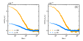
The behavior of correlations is also demonstrated in Fig S3: Without a capturing mechanism, correlations are purely negative due to the creation of empty sites resulting from the processive polymerization scheme. Opposed to that, purely positive correlations arise in a static lattice with capturing.
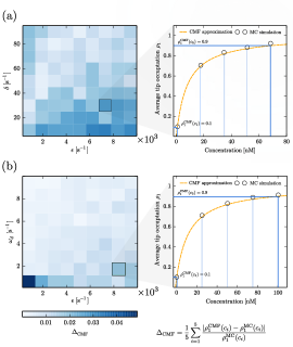
The CMF approach neglects correlations within the diffusive compartment (i.e. we assume and for and ). As this approximation is a non-perturbative ansatz, it is in general not possible to quantify its error. In order to ensure the validity over a broad and biologically relevant parameter range, we performed extensive MC simulations and compared the result with CMF computations. In detail, we performed parameter sweeps for (from ), (from ), (from ) and (for each parameter point at five equidistant values between and , such that and ). The results are shown in Fig. S4. The CMF approximation delivers good results over this very broad parameter range; the maximum relative deviation for over the 1000 different tested parameter sets is 6.5%.
In a previous publication, we derived an effective theory that allows for the calculation of reaction site occupations that are subject to a diffusion and capture mechanism in a static lattice (i.e. without lattice growth or shrinkage) Reithmann2015. While both approaches consider protein diffusion and capture on filaments, they differ significantly on a conceptual level and with respect to the scope of their predictions: Whereas the previous approach is based an on a heuristic theory and a priori only valid in the absence of polymerization and depolymerization, respectively, the CMF approach specifically accounts for lattice growth and shrinkage. Further, the CMF approximation is derived from more conceptual considerations: It assumes that diffusion and capture creates correlations which primarily affect the tip occupation while the diffusive motion of proteins on the MT depends less significantly on mutual correlations Derrida2007. As a consequence, the CMF approach yields density and tip-bulk correlation profiles for protein occupations along the MT, which are beyond the scope of our previous approach. As shown in the main text, the latter quantities are key to a quantitative understanding of tip-localization due to diffusion and capture and related processes.
V Uncatalyzed growth and shrinkage of MTs
The model described in the main text does not account for MT growth or shrinkage in the absence of depolymerziation or polymerization factors like MCAK or XMAP215. The reason for this assumption is twofold: a) In the experiments with XMAP215 Widlund2011 and MCAK Cooper2010 low concentrations of free tubulin were used such that no spontaneous MT growth was observed. Also, the measurements in Widlund et al. Widlund2011 suggest that the rate of tubulin detachment in the corresponding experiments is negligible. b) Concerning MT depolymerization, we aim for a description of protein induced tubulin removal from stabilized MTs in analogy to in vitro experiments with MCAK Cooper2010; Helenius2006. In this way, our model neglects the dynamic instability seen for unstabilized MTs Antal2007; Padinhateeri2012; Niedermayer2015; Zakharov2015, but provides a description how a stabilizing structure at the MT tip (e.g. GTP-tubulin) can be removed by regulatory enzymes.
That being said, let us emphasize that an extension towards uncatalyzed tubulin attachment and detachment is feasible based on the model described in the main text. To this end we include further processes in the model: If the terminal lattice site is unoccupied, a new site can be added at rate or removed at rate . For completeness, we also include catalyzed (processive) growth and shrinkage with corresponding rates and , respectively. The resulting equations for the CMF framework then read
| (S12) | |||||
| (S13) | |||||
| (S14) | |||||
| (S16) | |||||
The equations are solved in analogy to the case without spontaneous lattice dynamics.
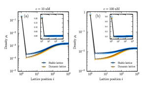
As mentioned above, our models neglect intrinsic MT dynamics such as dynamic instability. However, we expect validity of our results for tip-localization also under such circumstances. We studied the extended model with spontaneous growth and shrinkage rates over a variety of parameter values (up to spontaneous growth and shrinkage rates of ). For a comparison, we estimated the rate of spontaneous MT growth () at tubulin concentrations slightly above 5 from the experiments performed by Widlund et al. Widlund2011. At such tubulin concentrations, MTs were observed to start growing also without the presence of XMAP215 at a speed of approximately . Given this resulting spontaneous MT growth rate, we compared a model with and without fast intrinsic MT dynamics ( and for a stable lattice; and for a dynamic lattice). The results are shown in Figs. S5 and S6. They show the robustness of the protein distribution and, in particular, the tip occupation against changes in the lattice growth or shrinkage rates. Moreover, the CMF approximation is also applicable for rapidly fluctuating MT lengths. Note that XMAP215 also catalyzes tubulin removal under certain conditions Brouhard2008 which could readily be accounted for in the above approach.
VI MCAK model
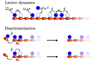
Similar to the model for XMAP215 stated in the main text we can set up a model for the depolymerase activity of MCAK, see Fig. S7. The ensuing set of equations corresponding to the CMF approach in the bulk are a special case of Eqs. S12-S16 with . We implement a processive depolymerization scheme Helenius2006; Cooper2010; Klein2005. In detail, MCAK particles stay at the terminal site during depolymerization (i.e. move along with the tip) whenever the neighboring site is empty. Otherwise, they dissociate from the tip during depolymerization. This means that MCAK particles fall off the MT tip whenever they hit another particle during the depolymerization process.
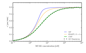
The results of the CMF approach for the MCAK model agree excellently with simulation data, as shown in Fig. S8. Further, also for the MCAK model the MF approximation and FSMFT produce results that deviate from simulation data at intermediate concentrations.
VII Parameter values
| Experiment | |||||
| (m) | events /(s m nM) | events/s | m/min | m/(min nM) | |
| MCAK-FL | 7.6 | 4.56 | 1.70 | 5.0 | 4.3 |
| (m) | events /(s m nM) | events/s | m/min | s-1 | |
| XMAP215 | 3.0 | 1 | 4.1 | 4.6 | 2.6 |
| Theory | |||||
| MCAK-FL | 1.2 | 2.61 | 1.70 | 5.2 | 3.0 |
| XMAP215 | 4.7 | 6 | 4.1 | 9.5 | 2.6 |
The parameter values used for the XMAP215 and MCAK model were extracted from experimental data Cooper2010; Brouhard2008; Widlund2011. Model parameters were computed based on measured diffusion coefficients (for ), particle dwell times on the MT tip (for ) and bulk (for ), attachment rates (for ), and maximal (de)polymerization velocities at saturated (de)polymerase concentrations (for ). A conversion factor from into tubulin subunits was adapted to the assumed protofilament numbers of the MTs used in the respective experiments: 1625 for XMAP215 Widlund2011 and 1750 for MCAK Cooper2010. Note that the polymerization velocity refers to one MT tip Brouhard2008; Widlund2011, wheres the depolymerization rate refers to the average shrinkage rate of both ends Cooper2010. Opposed to the measurements for MCAK, where the maximal depolymerization velocity was determined Cooper2010, Widlund et al. do not directly state the maximal MT polymerization velocity due to XMAP215 induced growth Widlund2011. To get a good estimate for the maximal growing velocity of MTs at saturating polymerase (XMAP215) concentrations, we fitted a Michaelis-Menten curve to the experimental data. The rate of tubulin attachment and detachment per regulating protein depends on the maximal number of catalytically active proteins at the MT tip : . Since the specific number for is elusive (there are estimates for approximately 10 XMAP215s at the MT tip at XMAP215. Brouhard2008), we have to make an assumption. Here, we choose one protein per protofilament, . In doing so the MT tip velocity then reduces to , where is the length of a tubulin dimer.
As the dwell time of proteins on the tip (i.e. ) was not measured for MCAK particles, we used the measured Michaelis constant to estimate this value: Since the Michaelis constant determines the linear increase in the depolymerization velocity for asymptotically low MCAK concentrations, , we can use it to estimate the tip-dwell time for MCAK particles. In detail, we analytically computed the depolymeriztion velocity for asymptotically low concentrations using a MF and low-density approximation of our model up to first order in Reithmann2015. As correlations vanish under these conditions, we expect the result to be exact which allows us to infer the MCAK off-rate at the tip . The list of ensuing parameters is given in Table 1.
References
- Reithmann et al. (2015) E. Reithmann, L. Reese, and E. Frey, Biophys. J. 108, 787 (2015).
- Derrida (2007) B. Derrida, J. Stat. Mech. Theor. Exp. 2007, P07023 (2007).
- Widlund et al. (2011) P. O. Widlund, J. H. Stear, A. Pozniakovsky, M. Zanic, S. Reber, G. J. Brouhard, A. A. Hyman, and J. Howard, Proc. Nat. Acad. Sci. USA 108, 2741 (2011).
- Cooper et al. (2010) J. R. Cooper, M. Wagenbach, C. L. Asbury, and L. Wordeman, Nat. Struct. Mol. Biol. 17, 77 (2010).
- Helenius et al. (2006) J. Helenius, G. J. Brouhard, Y. Kalaidzidis, S. Diez, and J. Howard, Nature 441, 115 (2006).
- Antal et al. (2007) T. Antal, P. L. Krapivsky, S. Redner, M. Mailman, and B. Chakraborty, Phys. Rev. E 76, 041907 (2007).
- Padinhateeri et al. (2012) R. Padinhateeri, A. B. Kolomeisky, and D. Lacoste, Biophys. J. 102, 1274 (2012).
- Niedermayer and Lipowsky (2015) T. Niedermayer and R. Lipowsky, Phys. Rev. E 92, 052137 (2015).
- Zakharov et al. (2015) P. Zakharov, N. Gudimchuk, V. Voevodin, A. Tikhonravov, F. I. Ataullakhanov, and E. L. Grishchuk, Biophys. J. 109, 2574 (2015).
- Brouhard et al. (2008) G. J. Brouhard, J. H. Stear, T. L. Noetzel, J. Al-Bassam, K. Kinoshita, S. C. Harrison, J. Howard, and A. A. Hyman, Cell 132, 79 (2008).
- Klein et al. (2005) G. Klein, K. Kruse, G. Cuniberti, and F. Jülicher, Phys. Rev. Lett. 94, 108102 (2005).