Shocks, rarefaction waves, and current fluctuations
for anharmonic chains

Christian B. Mendl111Geballe Laboratory for Advanced Materials, Stanford University, 476 Lomita Mall, California 94305, and Stanford Institute for Materials and Energy Sciences, SLAC National Accelerator Laboratory, Menlo Park, California 94025, USA. Email: mendl@stanford.edu   and Herbert Spohn222Zentrum Mathematik and Physik Department, Technische Universität München, Boltzmannstraße 3, 85747 Garching bei München, Germany. Email: spohn@tum.de
(July 14, 2016)
Abstract

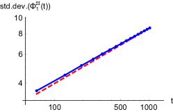
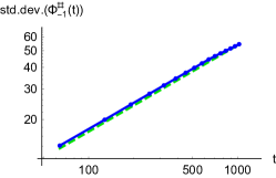
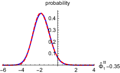
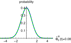
The nonequilibrium dynamics of anharmonic chains is studied by imposing an initial domain-wall state, in which the two half lattices are prepared in equilibrium with distinct parameters. We analyse the Riemann problem for the corresponding Euler equations and, in specific cases, compare with molecular dynamics. Additionally, the fluctuations of time-integrated currents are investigated. In analogy with the KPZ equation, their typical fluctuations should be of size t1/3superscript𝑡13t^{1/3} and have a Tracy-Widom GUE distributed amplitude. The proper extension to anharmonic chains is explained and tested through molecular dynamics. Our results are calibrated against the stochastic LeRoux lattice gas.

1 Introduction

The cold atom community has revived the study of the approach to thermal equilibrium for large isolated quantum systems. We refer to [1, 2] and references therein on previous work. Most accessible, both numerically and experimentally, are lattice systems in one dimension. One dimension is peculiar, since there are models with an extensive number of locally conserved fields. Examples of such quantum integrable systems are the XXZ spin chain and the continuum Lieb-Liniger δ𝛿\delta-Bose gas. Obviously the pathway to equilibrium will depend crucially on whether the system is integrable or not [3, 4, 5]. But in addition there is also the dependence on initial conditions which is potentially overwhelming. One could prepare the system already in thermal equilibrium and study the response to small initial perturbations [6]. These are the much investigated time response and correlation functions in equilibrium. The initial state could be translation invariant, to some extent thereby suppressing the mostly slow spatial variations [3]. Recently initial domain-wall states have become very popular [7, 8]. Such a state is obtained by joining two distinct thermal states at a single point (and at two points in case of periodic boundary conditions). Domain-wall states will be the main focus of our contribution.

Browsing the introductions to the papers mentioned above, one might have the impression that the approach to equilibrium for classical systems in one dimension is a well-covered topic. We study here Fermi-Pasta-Ulam type anharmonic chains with domain-wall initial conditions and are not aware of any previous systematic study. The structure of equilibrium time-correlations for such chains has been elucidated only recently [9, 10]. In particular one now understands the link to anomalous transport which is most directly observed when coupling the chain to thermal reservoirs at distinct temperatures, see [11]. As in the quantum world, there are integrable chains, in our context the most famous one being the Toda chain. But the KAM theorem signals in addition the possibility that, as a function of the energy, the structure may change from integrable to chaotic. This energy threshold is fascinating from the perspective of nonlinear dynamics and has attracted considerable attention [12]. We hope that a better understanding of classical models also serves as an incentive to look for related phenomena in quantum systems.

The parameters of the initial domain-wall state will be chosen such that in the accessible part of phase space the chain dynamics is sufficiently chaotic. Then one would expect that the conserved fields as computed from the chain dynamics are approximated by the respective solution of the macroscopic Euler equations, for times limited by diffusive effects. How well such expectations work out will have to be studied. The Euler equations are based on the notion of local thermodynamic equilibrium. The microscopic local conservation laws are deduced from the chain dynamics and are then averaged in the stipulated local equilibrium state so to arrive at a closed set of equations for the conserved fields. In particular, to reach non-trivial predictions, the thermal average of the microscopic currents is not allowed to vanish. This is ensured if the interaction potential depends only on positional differences, as V(qj+1qj)𝑉subscript𝑞𝑗1subscript𝑞𝑗V(q_{j+1}-q_{j}), implying momentum conservation. Upon adding an on-site potential, Vos(qj)subscript𝑉ossubscript𝑞𝑗V_{\mathrm{os}}(q_{j}), momentum conservation would be broken, all Euler currents would vanish, and the evolution of the initial step profile is determined by diffusive effects only.

The Euler equations are a system of n𝑛n hyperbolic conservation laws, n=3𝑛3n=3 for our case of anharmonic chains. They are of the generic form

tuα+x𝗃α(u)=0,subscript𝑡subscript𝑢𝛼subscript𝑥subscript𝗃𝛼𝑢0\partial_{t}u_{\alpha}+\partial_{x}\mathsf{j}_{\alpha}(\vec{u})=0, (1.1)

α=1,,n𝛼1𝑛\alpha=1,\dots,n, u=(u1,,un)𝑢subscript𝑢1subscript𝑢𝑛\vec{u}=(u_{1},\dots,u_{n}), with given current functions 𝗃𝗃\vec{\mathsf{j}}. In the mathematical literature the domain-wall initial data are known as Riemann problem for Eq. (1.1), which means

u(x,0)=u for x<0,u(x,0)=ur for x>0.formulae-sequence𝑢𝑥0subscript𝑢 for 𝑥0𝑢𝑥0subscript𝑢r for 𝑥0\vec{u}(x,0)=\vec{u}_{\ell}\text{ for }x<0,\qquad\vec{u}(x,0)=\vec{u}_{\mathrm{r}}\text{ for }x>0. (1.2)

For a wide class of current functions, there is a unique entropy solution to (1.1) with initial conditions (1.2), see the exposition [13], Sections 4–8. This solution scales ballistically as

u(x,t)=udw(x/t),𝑢𝑥𝑡subscript𝑢dw𝑥𝑡\vec{u}(x,t)=\vec{u}_{\mathrm{dw}}(x/t), (1.3)

where udwsubscript𝑢dw\vec{u}_{\mathrm{dw}} is bounded and continuous except for isolated jumps, possibly. There is a well developed theory of how to compute udwsubscript𝑢dw\vec{u}_{\mathrm{dw}}, at least in principle [13], Sections 1–3. In our case the current functions are determined through the microscopic particle model, and hence of a very particular form. Thus our task is twofold. Firstly we have to investigate the solution to the Riemann problem. Secondly such predictions should be compared with numerical simulations of the dynamics.

Let us return for a moment to the distinction between integrable and non-integrable systems, both starting from a domain-wall initial state. As supported by a variety of studies on quantum integrable models [3, 4], one expects that (1.3) still holds in the integrable case. Thus at first sight there seems to be little difference. Of course, the macroscopic profiles are computed by using completely different methods for the two cases. But the real distinguishing feature is the appearance of shocks. An ideal gas with step-initial conditions shows ballistic spreading but no shocks. The entropy solution for the Euler equations (1.1) is a mathematical shorthand for the limit of small dissipation, which is meaningful only if the underlying dynamics is sufficiently chaotic. Merely invoking the conservation laws, the Euler equations admit stable and unstable shocks. Such unphysical solutions to (1.1) are removed by requiring a positive entropy production at the shock, as will be illustrated in the examples below. In a local region away from the shock, the local state is (to very good approximation) in thermal equilibrium.

Our study adds current fluctuations as an item, which can no longer be based on the Euler equations (1.1). Most simple-mindedly, one would consider the fluctuations of the time-integrated current across the origin. For anharmonic chains the current is a three-vector. In most cases one would find Gaussian fluctuations of size t𝑡\sqrt{t}, thus not so interesting from a theoretical perspective. A more global picture emerges by considering the current integrated along the ray {x=𝗏t}𝑥𝗏𝑡\{x=\mathsf{v}t\} for some prescribed velocity 𝗏𝗏\mathsf{v}. The ray is chosen to lie in the interior of a rarefaction wave. In addition, one has to consider a computable but particular linear combination of the three currents. As will be discussed, then the integrated current fluctuations are of size t1/3superscript𝑡13t^{1/3}, smaller as for all other linear combinations, and the statistics is given by the Tracy-Widom distribution known from random matrix theory.

Our paper consists of three, at first sight somewhat unrelated parts. We start with a stochastic model with two conserved fields, as always with domain-wall initial conditions. For our particular system the validity of the Euler equations has been established mathematically [14]. Thus the model is used to explain the method by which one obtains the solution of the Riemann problem and as a numerical benchmark. We proceed to anharmonic chains, first with a general interaction potential. Analytically and numerically we then consider two specific choices for the potential, which generate sufficiently chaotic dynamics (as known from previous studies). In the third part we discuss the fluctuations of time-integrated currents.

2 Riemann problem for the LeRoux lattice gas

A prototypical stochastic lattice gas is the totally asymmetric simple exclusion process (TASEP). Particles are located on \mathbb{Z}, at most one particle per site. Independently, after an exponentially distributed waiting time, a particle hops one step to the right, provided the target site is empty. Clearly, the particle number is the only conserved field.

To move towards several conservation laws, we look for a minimal extension of the TASEP to a model with two conserved fields. In the literature a standard generalization is known as LeRoux stochastic lattice gas. (This name goes back to Fritz and Tóth [14], who prove the hydrodynamic limit globally in time. Apparently, LeRoux first wrote down this particular system of conservation laws [15, 16].) The LeRoux lattice gas has two types of particles with label ±1plus-or-minus1\pm 1. Subject to the exclusion rule, the 1 particles jump to the right and the 11-1 particles to the left, both according to the TASEP rule. Furthermore, a neighboring pair 1,1111,-1 is exchanged to 1,111-1,1 with rate 222, which leads to the simplification that the stationary measures are Bernoulli. A generalization of LeRoux is the Arndt-Heinzel-Rittenberg (AHR) model [17, 18].

More formally, we introduce occupation variables ηj=1,0,1subscript𝜂𝑗101\eta_{j}=-1,0,1, j𝑗j\in\mathbb{Z}. The only allowed exchanges are

1,0 0,11,\hskip 9.0pt0\ \to\ \hskip 7.0pt\,0,1 at  rate 1,
0,11,0formulae-sequence01100,-1\ \to\ -1,0 at  rate 1,
1,11,1formulae-sequence11111,-1\ \to\ -1,1 at  rate 2.

Note that in our convention the labels of the components are interchanged in comparison to [14]. Clearly, the only conserved fields are the two particle numbers. The invariant Bernoulli measures are parametrized by the average densities ρ1subscript𝜌1\rho_{1} and ρ1subscript𝜌1\rho_{-1}. The hydrodynamic equations simplify when written in terms of the average number of holes and the average velocity, i.e.,

ρ=1ρ1ρ1,v=ρ1ρ1formulae-sequence𝜌1subscript𝜌1subscript𝜌1𝑣subscript𝜌1subscript𝜌1\rho=1-\rho_{1}-\rho_{-1},\qquad v=\rho_{1}-\rho_{-1} (2.1)

with

|v|1,0ρ1|v|.formulae-sequence𝑣10𝜌1𝑣\lvert v\rvert\leq 1,\quad 0\leq\rho\leq 1-\lvert v\rvert. (2.2)

We refer to (ρ,v)𝜌𝑣(\rho,v) as states, more appropriately, but also more lengthy, as steady state parameters, resp. as thermodynamic states in case of anharmonic chains. The single-site probabilities of the steady states are

ρ,v(ηj=0)=ρ,ρ,v(ηj=±1)=12(1ρ±v).formulae-sequencesubscript𝜌𝑣subscript𝜂𝑗0𝜌subscript𝜌𝑣subscript𝜂𝑗plus-or-minus112plus-or-minus1𝜌𝑣\mathbbm{P}_{\rho,v}(\eta_{j}=0)=\rho,\qquad\mathbbm{P}_{\rho,v}(\eta_{j}=\pm 1)=\tfrac{1}{2}(1-\rho\pm v). (2.3)

Averages will be denoted by ρ,vsubscriptdelimited-⟨⟩𝜌𝑣\langle\cdot\rangle_{\rho,v}, the subscripts being omitted when obvious from the context. Since the steady states are of product form, their average current is easily computed. Thus, on a large space-time scale the conserved fields are governed by the entropy solution of

tu+x𝗃(u)=0,u=(ρ,v)formulae-sequencesubscript𝑡𝑢subscript𝑥𝗃𝑢0𝑢𝜌𝑣\partial_{t}\vec{u}+\partial_{x}\vec{\mathsf{j}}(\vec{u})=0,\quad\vec{u}=(\rho,v) (2.4)

with the current vector

𝗃(u)=(ρv,ρ+v21).𝗃𝑢𝜌𝑣𝜌superscript𝑣21\vec{\mathsf{j}}(\vec{u})=-(\rho\,v,\rho+v^{2}-1). (2.5)

To discuss the solution to the Riemann problem, we follow fairly closely the conventions of Ref. [13]. One rewrites (2.4) in semilinear form as

tu+A(u)xu=0,subscript𝑡𝑢𝐴𝑢subscript𝑥𝑢0\partial_{t}\vec{u}+A(\vec{u})\partial_{x}\vec{u}=0, (2.6)

where

A=𝗃(u)u=(vρ12v).𝐴𝗃𝑢𝑢matrix𝑣𝜌12𝑣A=\frac{\partial\vec{\mathsf{j}}(\vec{u})}{\partial\vec{u}}=-\begin{pmatrix}v&\rho\\ 1&2v\end{pmatrix}. (2.7)

The eigenvalues of A𝐴A are

cσ=32v+12σ4ρ+v2,σ=±1,formulae-sequencesubscript𝑐𝜎32𝑣12𝜎4𝜌superscript𝑣2𝜎plus-or-minus1c_{\sigma}=-\tfrac{3}{2}v+\tfrac{1}{2}\sigma\sqrt{4\rho+v^{2}},\qquad\sigma=\pm 1, (2.8)

and the corresponding right and left eigenvectors, Aψσ=cσψσ𝐴subscript𝜓𝜎subscript𝑐𝜎subscript𝜓𝜎A\psi_{\sigma}=c_{\sigma}\psi_{\sigma}, ATψ~σ=cσψ~σsuperscript𝐴Tsubscript~𝜓𝜎subscript𝑐𝜎subscript~𝜓𝜎A^{\mathrm{T}}\tilde{\psi}_{\sigma}=c_{\sigma}\tilde{\psi}_{\sigma}, are given by

ψσ=Zσ1(2σρσv4ρ+v2),ψ~σ=Z~σ1(2σσv4ρ+v2).formulae-sequencesubscript𝜓𝜎superscriptsubscript𝑍𝜎1matrix2𝜎𝜌𝜎𝑣4𝜌superscript𝑣2subscript~𝜓𝜎superscriptsubscript~𝑍𝜎1matrix2𝜎𝜎𝑣4𝜌superscript𝑣2\psi_{\sigma}=Z_{\sigma}^{-1}\begin{pmatrix}2\sigma\rho\\ \sigma v-\sqrt{4\rho+v^{2}}\end{pmatrix},\qquad\tilde{\psi}_{\sigma}=\tilde{Z}_{\sigma}^{-1}\begin{pmatrix}2\sigma\\ \sigma v-\sqrt{4\rho+v^{2}}\end{pmatrix}. (2.9)

Here Zσsubscript𝑍𝜎Z_{\sigma} and Z~σsubscript~𝑍𝜎\tilde{Z}_{\sigma} are positive normalization constants. For the Riemann problem their explicit form is not needed. Setting D=(ρ,v)𝐷subscript𝜌subscript𝑣D=(\partial_{\rho},\partial_{v}), one obtains for the change of cσsubscript𝑐𝜎c_{\sigma} along the vector fields ψσsubscript𝜓𝜎\psi_{\sigma},

ψσDcσ=2Zσ1(4ρ+v2σv)0,subscript𝜓𝜎𝐷subscript𝑐𝜎2superscriptsubscript𝑍𝜎14𝜌superscript𝑣2𝜎𝑣0\psi_{\sigma}\cdot Dc_{\sigma}=2\,Z_{\sigma}^{-1}\big{(}\sqrt{4\rho+v^{2}}-\sigma v\big{)}\geq 0, (2.10)

and strictly positive for ρ>0𝜌0\rho>0.

2.1 Rarefaction waves

The rarefaction curves, Rσsubscript𝑅𝜎R_{\sigma}, are obtained by solving the Cauchy problem in u𝑢\vec{u}-space,

τu=ψσ(u)subscript𝜏𝑢subscript𝜓𝜎𝑢\partial_{\tau}\vec{u}=\psi_{\sigma}(\vec{u}) (2.11)

for σ=±1𝜎plus-or-minus1\sigma=\pm 1, with ψσsubscript𝜓𝜎\psi_{\sigma} the right eigenvectors of A𝐴A, see (2.9). The normalization has been absorbed into the τ𝜏\tau-parameter. The integral curves are then determined by

τρ=2σρ,τv=σv4ρ+v2.formulae-sequencesubscript𝜏𝜌2𝜎𝜌subscript𝜏𝑣𝜎𝑣4𝜌superscript𝑣2\partial_{\tau}\rho=2\sigma\rho,\quad\partial_{\tau}v=\sigma v-\sqrt{4\rho+v^{2}}. (2.12)

It follows that

dvdρ=12σρ(4ρ+v2σv),𝑑𝑣𝑑𝜌12𝜎𝜌4𝜌superscript𝑣2𝜎𝑣\frac{dv}{d\rho}=-\frac{1}{2\sigma\rho}\big{(}\sqrt{4\rho+v^{2}}-\sigma v\big{)}, (2.13)

which is negative for R1subscript𝑅1R_{1} and positive for R1subscript𝑅1R_{-1}. The solution of (2.13) is

vσ=σ(bσbσ1ρ),0<bσ1,formulae-sequencesubscript𝑣𝜎𝜎subscript𝑏𝜎superscriptsubscript𝑏𝜎1𝜌0subscript𝑏𝜎1v_{\sigma}=\sigma\left(b_{\sigma}-b_{\sigma}^{-1}\rho\right),\qquad 0<b_{\sigma}\leq 1, (2.14)

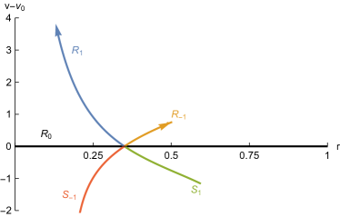
as visualized in Fig. 1. Maximally, R1subscript𝑅1R_{1} starts at u1,=(0,b1)subscript𝑢10subscript𝑏1\vec{u}_{1,\ell}=(0,b_{1}) and ends at u1,r=(b1,b11)subscript𝑢1rsubscript𝑏1subscript𝑏11\vec{u}_{1,\mathrm{r}}=(b_{1},b_{1}-1), whereas R1subscript𝑅1R_{-1} starts at u1,=(b1,1b1)subscript𝑢1subscript𝑏11subscript𝑏1\vec{u}_{-1,\ell}=(b_{-1},1-b_{-1}) and ends at u1,r=(0,b1)subscript𝑢1r0subscript𝑏1\vec{u}_{-1,\mathrm{r}}=(0,-b_{-1}). The local eigenvalue is

cσ=32v+12σ4ρ+v2=σ(bσ12ρbσ).subscript𝑐𝜎32𝑣12𝜎4𝜌superscript𝑣2𝜎superscriptsubscript𝑏𝜎12𝜌subscript𝑏𝜎c_{\sigma}=-\tfrac{3}{2}v+\tfrac{1}{2}\sigma\sqrt{4\rho+v^{2}}=\sigma\left(b_{\sigma}^{-1}2\rho-b_{\sigma}\right). (2.15)

To convert the solution from u𝑢\vec{u}-space to position space, we set cσ=x/tsubscript𝑐𝜎𝑥𝑡c_{\sigma}=x/t. The solution is self-similar and we may assume t=1𝑡1t=1. Then

ρσ(x)=12bσ(bσ+σx),vσ(x)=12(bσσx).formulae-sequencesubscript𝜌𝜎𝑥12subscript𝑏𝜎subscript𝑏𝜎𝜎𝑥subscript𝑣𝜎𝑥12subscript𝑏𝜎𝜎𝑥\rho_{\sigma}(x)=\tfrac{1}{2}b_{\sigma}(b_{\sigma}+\sigma x),\quad v_{\sigma}(x)=\tfrac{1}{2}(b_{\sigma}-\sigma x). (2.16)

The boundary speeds of R1subscript𝑅1R_{1} are

c1,=c1(u1,)=b1,c1,r=c1(u1,r)=2b1,formulae-sequencesubscript𝑐1subscript𝑐1subscript𝑢1subscript𝑏1subscript𝑐1rsubscript𝑐1subscript𝑢1r2subscript𝑏1c_{1,\ell}=c_{1}(\vec{u}_{1,\ell})=-b_{1},\quad c_{1,\mathrm{r}}=c_{1}(\vec{u}_{1,\mathrm{r}})=2-b_{1}, (2.17)

and of R1subscript𝑅1R_{-1}

c1,=c1(u1,)=b12,c1,r=c1(u1,r)=b1.formulae-sequencesubscript𝑐1subscript𝑐1subscript𝑢1subscript𝑏12subscript𝑐1rsubscript𝑐1subscript𝑢1rsubscript𝑏1c_{-1,\ell}=c_{-1}(\vec{u}_{-1,\ell})=b_{-1}-2,\quad c_{-1,\mathrm{r}}=c_{-1}(\vec{u}_{-1,\mathrm{r}})=b_{-1}. (2.18)

Eq. (2.16) as a function of x/t𝑥𝑡x/t describes solutions of the Euler equation (2.4). The two solutions with σ=±1𝜎plus-or-minus1\sigma=\pm 1 are mirror images of each other.

Refer to caption
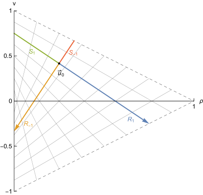
Figure 1: Rarefaction and shock curves through a point u0subscript𝑢0\vec{u}_{0} in state space for the LeRoux system according to Eqs. (2.14) and (2.26). Traversal in arrow direction corresponds to a rarefaction wave and increasing cσsubscript𝑐𝜎c_{\sigma}, and traversal in opposite arrow direction to a shock curve.

2.2 Shock curves

Shock curves are determined by the Rankine-Hugoniot jump condition

λ(uu0)=𝗃(u)𝗃(u0).𝜆𝑢subscript𝑢0𝗃𝑢𝗃subscript𝑢0\lambda(\vec{u}-\vec{u}_{0})=\vec{\mathsf{j}}(\vec{u})-\vec{\mathsf{j}}(\vec{u}_{0}). (2.19)

Hence in our case

λ(ρρ0)𝜆𝜌subscript𝜌0\displaystyle-\lambda(\rho-\rho_{0}) =ρvρ0v0,absent𝜌𝑣subscript𝜌0subscript𝑣0\displaystyle=\rho v-\rho_{0}v_{0}, (2.20)
λ(vv0)𝜆𝑣subscript𝑣0\displaystyle-\lambda(v-v_{0}) =ρρ0+v2v02.absent𝜌subscript𝜌0superscript𝑣2superscriptsubscript𝑣02\displaystyle=\rho-\rho_{0}+v^{2}-v_{0}^{2}. (2.21)

According to the first equation the shock speed is

λ=ρvρ0v0ρρ0.𝜆𝜌𝑣subscript𝜌0subscript𝑣0𝜌subscript𝜌0\lambda=-\frac{\rho v-\rho_{0}v_{0}}{\rho-\rho_{0}}. (2.22)

We eliminate λ𝜆\lambda with the result

(ρρ0)2=(vv0)(vρ0v0ρ).superscript𝜌subscript𝜌02𝑣subscript𝑣0𝑣subscript𝜌0subscript𝑣0𝜌(\rho-\rho_{0})^{2}=(v-v_{0})(v\rho_{0}-v_{0}\rho). (2.23)

If ρ0>0subscript𝜌00\rho_{0}>0, the two solutions for v𝑣v are

vσ=v0+(1ρ^)(cσ,0+v0),ρ^=ρ/ρ0formulae-sequencesubscript𝑣𝜎subscript𝑣01^𝜌subscript𝑐𝜎0subscript𝑣0^𝜌𝜌subscript𝜌0v_{\sigma}=v_{0}+(1-\hat{\rho})(c_{\sigma,0}+v_{0}),\quad\hat{\rho}=\rho/\rho_{0} (2.24)

with σ=±1𝜎plus-or-minus1\sigma=\pm 1 and cσ,0=cσ(u0)subscript𝑐𝜎0subscript𝑐𝜎subscript𝑢0c_{\sigma,0}=c_{\sigma}(\vec{u}_{0}) the sound speed (2.8) on the left side of the shock. In particular, one recovers vσ=v0subscript𝑣𝜎subscript𝑣0v_{\sigma}=v_{0} for ρ^=1^𝜌1\hat{\rho}=1. In fact, the rarefaction curves (2.14) coincide with the solution to the Rankine-Hugoniot equations (2.24). This can be seen by defining bσsubscript𝑏𝜎b_{\sigma} implicitly via

vσ,0=σ(bσbσ1ρ0),subscript𝑣𝜎0𝜎subscript𝑏𝜎superscriptsubscript𝑏𝜎1subscript𝜌0v_{\sigma,0}=\sigma\left(b_{\sigma}-b_{\sigma}^{-1}\rho_{0}\right), (2.25)

then

vσ=σ(bσbσ1ρ).subscript𝑣𝜎𝜎subscript𝑏𝜎superscriptsubscript𝑏𝜎1𝜌v_{\sigma}=\sigma\left(b_{\sigma}-b_{\sigma}^{-1}\rho\right). (2.26)

Inserting into (2.22) one arrives at the shock speed

λσ=12(cσ,0+cσ)=σ(bσ1(ρ+ρ0)bσ).subscript𝜆𝜎12subscript𝑐𝜎0subscript𝑐𝜎𝜎superscriptsubscript𝑏𝜎1𝜌subscript𝜌0subscript𝑏𝜎\lambda_{\sigma}=\tfrac{1}{2}(c_{\sigma,0}+c_{\sigma})=\sigma\left(b_{\sigma}^{-1}(\rho+\rho_{0})-b_{\sigma}\right). (2.27)

The coincidence of rarefaction and shock curves is the defining property of the Temple class [19]. The LeRoux system is a further member of this class. In our context the interest results from a maximally simple underlying particle dynamics.

The Lax admissibility condition states that characteristics must move “towards” the shock:

cσ,0λcσ.subscript𝑐𝜎0𝜆subscript𝑐𝜎c_{\sigma,0}\geq\lambda\geq c_{\sigma}. (2.28)

Since λ𝜆\lambda is the mean value of the sound speeds, the condition simplifies to cσcσ,0subscript𝑐𝜎subscript𝑐𝜎0c_{\sigma}\leq c_{\sigma,0}. Together with cσ=σ(b12ρb)subscript𝑐𝜎𝜎superscript𝑏12𝜌𝑏c_{\sigma}=\sigma(b^{-1}2\rho-b), this is equivalent to ρρ0𝜌subscript𝜌0\rho\leq\rho_{0} for σ=1𝜎1\sigma=1 and ρρ0𝜌subscript𝜌0\rho\geq\rho_{0} for σ=1𝜎1\sigma=-1. The stable, physically admissible part of the Rankine-Hugoniot curve are the shock curves S1subscript𝑆1S_{1} and S1subscript𝑆1S_{-1} as displayed in Fig 1.

2.3 General solution

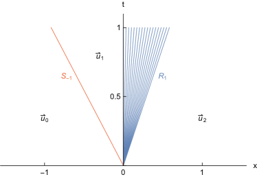
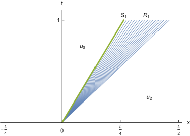
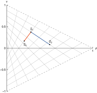
The construction of the general solution is illustrated in Fig. 2. Starting from the asymptotic left value u=u0subscript𝑢subscript𝑢0\vec{u}_{\ell}=\vec{u}_{0}, one first follows either the rarefaction curve R1subscript𝑅1R_{-1} or the stable part of the shock curve S1subscript𝑆1S_{-1} (shown as linear orange-red line in Fig. 1) up to a unique intermediate state u1subscript𝑢1\vec{u}_{1}. Then u1subscript𝑢1\vec{u}_{1} is connected by either a rarefaction curve R1subscript𝑅1R_{1} or shock curve S1subscript𝑆1S_{1} (blue-green in Fig. 1) to the asymptotic right value u2=ursubscript𝑢2subscript𝑢r\vec{u}_{2}=\vec{u}_{\mathrm{r}}. Rarefaction curves correspond to traversal in arrow direction in Fig. 1, equivalently increasing eigenvalue cσsubscript𝑐𝜎c_{\sigma}. This procedure splits the parameter domain into four distinct pieces according to rarefaction-rarefaction, shock-rarefaction, rarefaction-shock, and shock-shock. The two domain boundaries correspond to either a single rarefaction or a single shock, with no intermediate value u1subscript𝑢1\vec{u}_{1}. In Fig. 2b we show the space-time plot corresponding to the case shock-rarefaction of Fig. 2a.
Refer to caption
(a) path in state space
Refer to caption
(b) corresponding shock and rarefaction wave
Figure 2: (a) Path in state space from initial state u0subscript𝑢0\vec{u}_{0} via u1subscript𝑢1\vec{u}_{1} to the final state u2subscript𝑢2\vec{u}_{2}, traversing along the red shock curve S1subscript𝑆1S_{-1} first and then along the blue rarefaction curve R1subscript𝑅1R_{1}. (b) Corresponding shock and rarefaction waves in a x𝑥x-t𝑡t diagram.

2.4 Monte Carlo simulations

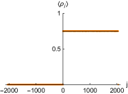
We perform Monte Carlo simulations of the LeRoux model for L=4096𝐿4096L=4096 sites with periodic boundary conditions. To obtain an initial domain wall state, we sample the single-site probability distribution (2.3) on the left half j=L2,,1𝑗𝐿21j=-\frac{L}{2},\dots,-1 using parameters u=(ρ,v)subscript𝑢subscript𝜌subscript𝑣\vec{u}_{\ell}=(\rho_{\ell},v_{\ell}), and on the right half j=0,,L21𝑗0𝐿21j=0,\dots,\frac{L}{2}-1 using parameters ur=(ρr,vr)subscript𝑢rsubscript𝜌rsubscript𝑣r\vec{u}_{\mathrm{r}}=(\rho_{\mathrm{r}},v_{\mathrm{r}}). The dynamics is simulated by random exchanges at exponentially distributed waiting times up to tmax=1024subscript𝑡1024t_{\max}=1024. This procedure is realized 106superscript10610^{6} times to compute average profiles, as shown below.
Refer to caption
(a) density, t=0𝑡0t=0
Refer to caption
(b) density, t=256𝑡256t=256
Refer to caption
(c) density, t=512𝑡512t=512
Refer to caption
(d) density, t=1024𝑡1024t=1024
Refer to caption
(e) velocity, t=0𝑡0t=0
Refer to caption
(f) velocity, t=256𝑡256t=256
Refer to caption
(g) velocity, t=512𝑡512t=512
Refer to caption
(h) velocity, t=1024𝑡1024t=1024
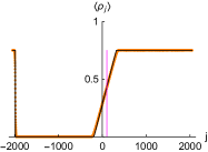
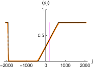
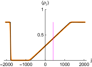
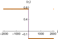
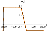
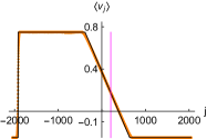
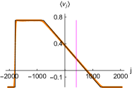
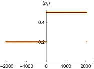
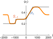
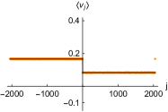
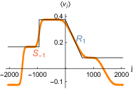
Figure 3: Density and velocity profiles at various times for the LeRoux model with domain-wall initial conditions u=(0,b1)subscript𝑢0subscript𝑏1\vec{u}_{\ell}=(0,b_{1}) and ur=(b1,b11)subscript𝑢rsubscript𝑏1subscript𝑏11\vec{u}_{\mathrm{r}}=(b_{1},b_{1}-1), b1=34subscript𝑏134b_{1}=\frac{3}{4} and L=4096𝐿4096L=4096 sites. The orange dots are molecular dynamics results and the black line shows the theoretically predicted profile. The sharp jump on the left is a shock resulting from the periodic boundary conditions, and the sloped linear segment is a rarefaction wave.
Refer to caption
(a) density, t=0𝑡0t=0
Refer to caption
(b) density, t=256𝑡256t=256
Refer to caption
(c) density, t=512𝑡512t=512
Refer to caption
(d) density, t=1024𝑡1024t=1024
Refer to caption
(e) velocity, t=0𝑡0t=0
Refer to caption
(f) velocity, t=256𝑡256t=256
Refer to caption
(g) velocity, t=512𝑡512t=512
Refer to caption
(h) velocity, t=1024𝑡1024t=1024
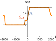
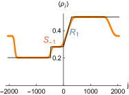
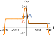
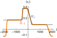
Figure 4: Density and velocity profiles at various times for the LeRoux model with domain-wall initial conditions corresponding to Fig. 2. The shock wave S1subscript𝑆1S_{-1} and rarefaction wave R1subscript𝑅1R_{1} are indicated in red and blue, respectively. The theoretical prediction (black lines) refers only to the Riemann problem centered at the origin. The outer features of the MC profiles arise from periodic boundary conditions.

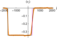
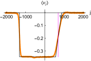
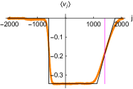
First, we illustrate the special case of a single rarefaction wave R1subscript𝑅1R_{1} connecting usubscript𝑢\vec{u}_{\ell} to ursubscript𝑢r\vec{u}_{\mathrm{r}}, which are chosen maximally as u=(0,b1)subscript𝑢0subscript𝑏1\vec{u}_{\ell}=(0,b_{1}) and ur=(b1,b11)subscript𝑢rsubscript𝑏1subscript𝑏11\vec{u}_{\mathrm{r}}=(b_{1},b_{1}-1) with b1=34subscript𝑏134b_{1}=\frac{3}{4}. This is the particular choice in [20], and corresponds to the extremal points of the green-blue line segment in Fig. 1. Besides the u|urconditionalsubscript𝑢subscript𝑢r\vec{u}_{\ell}|\vec{u}_{\mathrm{r}} Riemann problem centered at j=0𝑗0j=0 and generating rarefaction R1subscript𝑅1R_{1}, the periodic boundary condition translates to an additional ur|uconditionalsubscript𝑢rsubscript𝑢\vec{u}_{\mathrm{r}}|\vec{u}_{\ell} Riemann problem centered at j=L2𝑗𝐿2j=\frac{L}{2}. Since the solutions of the rarefaction and shock curves coincide except for orientation, one concludes that the solution of the ur|uconditionalsubscript𝑢rsubscript𝑢\vec{u}_{\mathrm{r}}|\vec{u}_{\ell} Riemann problem is a single shock curve S1subscript𝑆1S_{1}. In other words, one traverses the green-blue line segment in Fig. 1 in opposite direction. The numerical Monte Carlo profiles, shown as orange dots in Fig. 3, agree very well with the theoretical prediction (solid black lines). In particular, note the sharp jump at the shock. This shock curve is located at j=L2+λ1t𝑗𝐿2subscript𝜆1𝑡j=-\frac{L}{2}+\lambda_{1}t and moves to the right, with shock speed λ1=1b1subscript𝜆11subscript𝑏1\lambda_{1}=1-b_{1}.

Next, we perform molecular dynamics simulations corresponding to the general case in Fig. 2. Specifically, the left u=u0=(1364,16)subscript𝑢subscript𝑢0136416\vec{u}_{\ell}=\vec{u}_{0}=(\frac{13}{64},\frac{1}{6}), the intermediate u1=(932,38)subscript𝑢193238\vec{u}_{1}=(\frac{9}{32},\frac{3}{8}) and the right ur=u2=(12,112)subscript𝑢rsubscript𝑢212112\vec{u}_{\mathrm{r}}=\vec{u}_{2}=(\frac{1}{2},\frac{1}{12}). Fig. 4 shows the molecular dynamics profiles, with the shock curve S1subscript𝑆1S_{-1} indicated in red and the rarefaction wave R1subscript𝑅1R_{1} in blue. One observes that the MC profile of S1subscript𝑆1S_{-1} is less sharp than the shock in Fig. 3, presumably due to the higher shock speed.

2.5 Entropy

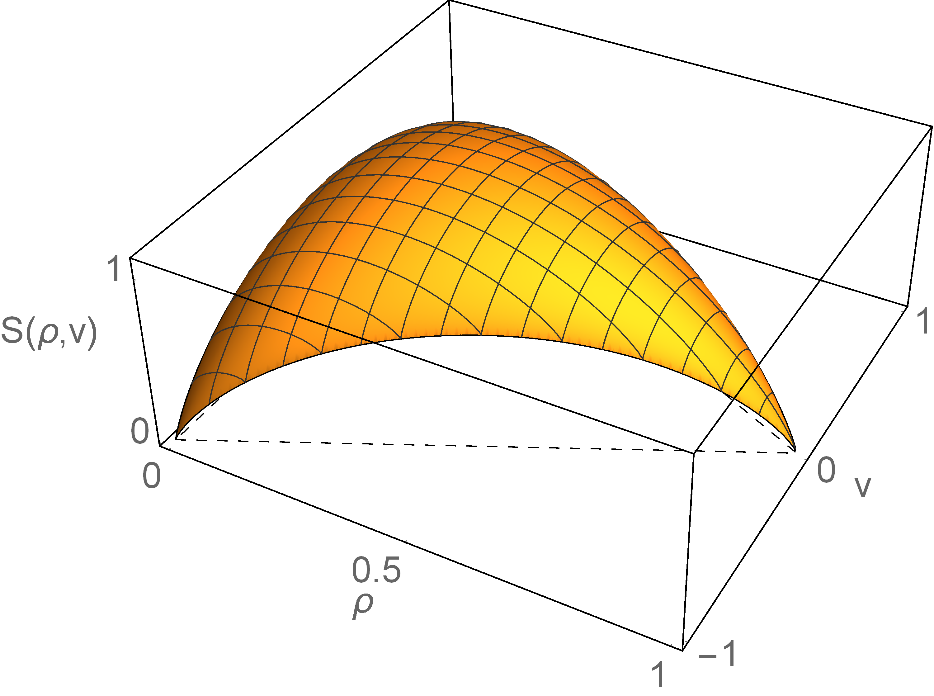
The thermodynamic entropy for the probability distribution of (2.3) is

S(ρ,v)=η=11ρ,v(η)logρ,v(η),𝑆𝜌𝑣superscriptsubscript𝜂11subscript𝜌𝑣𝜂subscript𝜌𝑣𝜂S(\rho,v)=-\sum_{\eta=-1}^{1}\mathbbm{P}_{\rho,v}(\eta)\log\mathbbm{P}_{\rho,v}(\eta), (2.29)

using the standard physics convention for the sign. The definition in [13] uses a convex function which has the opposite sign.
Refer to caption
(a) entropy S(q,v)𝑆𝑞𝑣S(q,v)
Refer to caption
(b) entropy flux q(ρ,v)𝑞𝜌𝑣q(\rho,v)
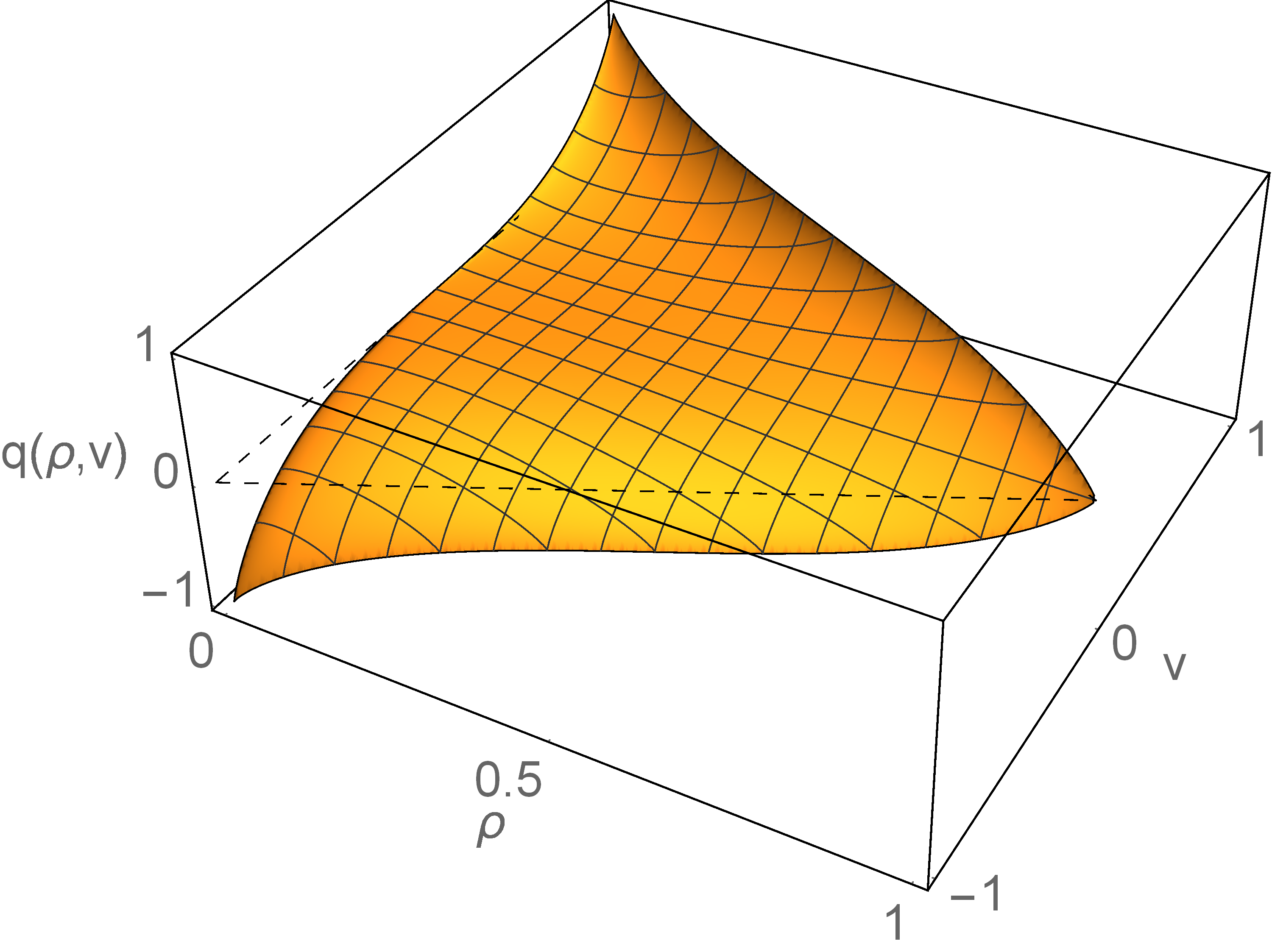
Figure 5: Entropy according to Eq. (2.29) and entropy flux according to Eq. (2.31) of the LeRoux model.

The corresponding entropy flux q(u)𝑞𝑢q(\vec{u}) has to satisfy

DS(u)A=Dq(u)𝐷𝑆𝑢𝐴𝐷𝑞𝑢DS(\vec{u})\,A=Dq(\vec{u}) (2.30)

with u=(ρ,v)𝑢𝜌𝑣\vec{u}=(\rho,v) and D=(ρ,v)𝐷subscript𝜌subscript𝑣D=(\partial_{\rho},\partial_{v}). Up to a constant the solution for q(u)𝑞𝑢q(\vec{u}) is

q(ρ,v)=v+η=11(vη)ρ,v(η)logρ,v(η).𝑞𝜌𝑣𝑣superscriptsubscript𝜂11𝑣𝜂subscript𝜌𝑣𝜂subscript𝜌𝑣𝜂q(\rho,v)=v+\sum_{\eta=-1}^{1}(v-\eta)\mathbbm{P}_{\rho,v}(\eta)\log\mathbbm{P}_{\rho,v}(\eta). (2.31)

Note that q(ρ,v)𝑞𝜌𝑣q(\rho,v) is an odd function in v𝑣v. Fig. 5 visualizes both entropy and entropy flux.

The entropy inequality admissibility condition states that

tS(u)+xq(u)=ΔS(u)0subscript𝑡𝑆𝑢subscript𝑥𝑞𝑢Δ𝑆𝑢0\partial_{t}S(\vec{u})+\partial_{x}q(\vec{u})=\Delta S(\vec{u})\geq 0 (2.32)

in the sense of distributions. For continuously differentiable solutions due to (2.30) one has ΔS(u)=0Δ𝑆𝑢0\Delta S(\vec{u})=0 and

tS(u)+xq(u)=0.subscript𝑡𝑆𝑢subscript𝑥𝑞𝑢0\partial_{t}S(\vec{u})+\partial_{x}q(\vec{u})=0. (2.33)

In particular, no entropy is produced at a rarefaction wave. On the other side, at shocks one can follow the same steps as for the Rankine-Hugoniot jump condition to derive from (2.32) that

dt(λ(SS0)(qq0))ϕ(λt,t)=dtΔSϕ(λt,t)differential-d𝑡𝜆𝑆subscript𝑆0𝑞subscript𝑞0italic-ϕ𝜆𝑡𝑡differential-d𝑡Δ𝑆italic-ϕ𝜆𝑡𝑡-\int\mathrm{d}t\big{(}\lambda(S-S_{0})-(q-q_{0})\big{)}\phi(\lambda t,t)=\int\mathrm{d}t\,\Delta S\,\phi(\lambda t,t) (2.34)

for any continuously differentiable test function ϕ(x,t)italic-ϕ𝑥𝑡\phi(x,t) with compact support. The integration in (2.34) proceeds along the shock curve, and S0subscript𝑆0S_{0}, q0subscript𝑞0q_{0} are the values on the left side of the shock. Inserting the shock speed (2.27) and the shock solution into (2.29) and (2.31), one obtains (with b=bσ𝑏subscript𝑏𝜎b=b_{\sigma})

ΔSσ=σ(1b(ρ0ρ+ρρ0log[ρρ0])+1b(1b2(1ρ)(1ρ0))12log[1(ρ/b)21(ρ0/b)2](1ρρ0+ρρ0b2)(arctanh(ρ0b)arctanh(ρb))).Δsubscript𝑆𝜎𝜎1𝑏subscript𝜌0𝜌𝜌subscript𝜌0𝜌subscript𝜌01𝑏1superscript𝑏21𝜌1subscript𝜌0121superscript𝜌𝑏21superscriptsubscript𝜌0𝑏21𝜌subscript𝜌0𝜌subscript𝜌0superscript𝑏2arctanhsubscript𝜌0𝑏arctanh𝜌𝑏\Delta S_{\sigma}=\sigma\bigg{(}\frac{1}{b}\Big{(}\rho_{0}-\rho+\rho\,\rho_{0}\log\!\Big{[}\frac{\rho}{\rho_{0}}\Big{]}\Big{)}+\frac{1}{b}\left(1-b^{2}-(1-\rho)(1-\rho_{0})\right)\frac{1}{2}\log\!\left[\frac{1-(\rho/b)^{2}}{1-(\rho_{0}/b)^{2}}\right]\\ -\left(1-\rho-\rho_{0}+\frac{\rho\,\rho_{0}}{b^{2}}\right)\left(\mathrm{arctanh}\Big{(}\frac{\rho_{0}}{b}\Big{)}-\mathrm{arctanh}\Big{(}\frac{\rho}{b}\Big{)}\right)\bigg{)}. (2.35)

Note that this expression is invariant under the interchange ρρ0𝜌subscript𝜌0\rho\leftrightarrow\rho_{0} and simultaneously σσ𝜎𝜎\sigma\leftrightarrow-\sigma, as expected from symmetry of the shock curves moving to the right and left. As required, the solution of the Riemann problem satisfies ΔSσ0Δsubscript𝑆𝜎0\Delta S_{\sigma}\geq 0.

3 Riemann problem for anharmonic chains

With the LeRoux lattice gas as guiding example, we turn to our central theme which is the time evolution for domain-wall initial conditions of a system of anharmonically coupled mechanical point particles. The j𝑗j-th particle has mass m𝑚m, position qjsubscript𝑞𝑗q_{j}, momentum pjsubscript𝑝𝑗p_{j}, and is coupled to its neighbors j1𝑗1j-1 and j+1𝑗1j+1 through the potential V𝑉V. Then Newton’s equations of motion are given by

md2dt2qj=V(qj+1qj)V(qjqj1).𝑚superscriptd2dsuperscript𝑡2subscript𝑞𝑗superscript𝑉subscript𝑞𝑗1subscript𝑞𝑗superscript𝑉subscript𝑞𝑗subscript𝑞𝑗1m\tfrac{\mathrm{d}^{2}}{\mathrm{d}t^{2}}q_{j}=V^{\prime}(q_{j+1}-q_{j})-V^{\prime}(q_{j}-q_{j-1}). (3.1)

We read this equation as a discretized wave equation with qjsubscript𝑞𝑗q_{j}\in\mathbb{R} the displacement of the wave field at lattice site j𝑗j. The hamiltonian of the chain is

H=j(12mpj2+V(qj+1qj)).𝐻subscript𝑗12𝑚superscriptsubscript𝑝𝑗2𝑉subscript𝑞𝑗1subscript𝑞𝑗H=\sum_{j\in\mathbb{Z}}\big{(}\tfrac{1}{2m}p_{j}^{2}+V(q_{j+1}-q_{j})\big{)}. (3.2)

For the harmonic potential, V(x)=x2𝑉𝑥superscript𝑥2V(x)=x^{2}, Eq. (3.1) reduces to a discrete linear wave equation. In the theoretical analysis we use j𝑗j\in\mathbb{Z}. Numerically, j[L2,,L21]𝑗𝐿2𝐿21j\in[-\tfrac{L}{2},\dots,\tfrac{L}{2}-1] with periodic boundary conditions.

In contrast to the LeRoux lattice gas, the dynamics is deterministic. The initial conditions are however random, specifically to have a domain-wall state. As before, we expect the Euler equations to provide an accurate description on a macroscopic scale, provided the times are not too long. The validity of the Euler equations is based on maintaining local stationarity away from shocks. For a stochastic system the local approach to stationarity is in a certain sense build into the dynamics. For mechanical systems one relies on sufficiently strong dynamical chaos. Thereby integrable systems, as the harmonic and Toda chain are ruled out. In the LeRoux lattice gas the jumps are asymmetric. The steady states are non-equilibrium and the dynamics does not satisfy the principle of detailed balance. In contrast, for the anharmonic chain the domain-wall state is manufactured by joining two thermal equilibrium states. Because of momentum conservation, the thermal average defining the Euler currents does not vanish. If one broke this conservation law by adding in (3.2) an on-site potential, then the Euler currents would vanish identically, no Riemann problem ensues, and the first macroscopic time-scale is diffusive.

It is convenient to introduce the stretch rj=qj+1qjsubscript𝑟𝑗subscript𝑞𝑗1subscript𝑞𝑗r_{j}=q_{j+1}-q_{j}. Then the equations of motion turn into

ddtrj=1m(pj+1pj),ddtpj=V(rj)V(rj1),formulae-sequencedd𝑡subscript𝑟𝑗1𝑚subscript𝑝𝑗1subscript𝑝𝑗dd𝑡subscript𝑝𝑗superscript𝑉subscript𝑟𝑗superscript𝑉subscript𝑟𝑗1\tfrac{\mathrm{d}}{\mathrm{d}t}r_{j}=\tfrac{1}{m}(p_{j+1}-p_{j}),\qquad\tfrac{\mathrm{d}}{\mathrm{d}t}p_{j}=V^{\prime}(r_{j})-V^{\prime}(r_{j-1}), (3.3)

from which one concludes that stretch and momentum are conserved. The respective currents are 1mpj1𝑚subscript𝑝𝑗-\tfrac{1}{m}p_{j} and V(rj1)superscript𝑉subscript𝑟𝑗1-V^{\prime}(r_{j-1}). In addition, we define the local energy

ej=12mpj2+V(rj),subscript𝑒𝑗12𝑚superscriptsubscript𝑝𝑗2𝑉subscript𝑟𝑗e_{j}=\tfrac{1}{2m}p_{j}^{2}+V(r_{j}), (3.4)

which changes in time as

ddtej=1mpj+1V(rj)1mpjV(rj1).dd𝑡subscript𝑒𝑗1𝑚subscript𝑝𝑗1superscript𝑉subscript𝑟𝑗1𝑚subscript𝑝𝑗superscript𝑉subscript𝑟𝑗1\tfrac{\mathrm{d}}{\mathrm{d}t}e_{j}=\tfrac{1}{m}p_{j+1}V^{\prime}(r_{j})-\tfrac{1}{m}p_{j}V^{\prime}(r_{j-1}). (3.5)

As anticipated, the energy is locally conserved. Its current equals 1mpjV(rj1)1𝑚subscript𝑝𝑗superscript𝑉subscript𝑟𝑗1-\tfrac{1}{m}p_{j}V^{\prime}(r_{j-1}). More precisely than before, in our context non-integrable means that there are no further locally conserved fields. Unfortunately, this property is difficult to check. Besides the harmonic chain, the only known integrable system is the Toda chain with V(x)=ex𝑉𝑥superscripte𝑥V(x)=\mathrm{e}^{-x}. [The Calogero-Moser chain has a two-sided decaying potential, which is not allowed in our context.]

The thermodynamic fields conjugate to stretch, momentum, and energy are the pressure P𝑃P, the mean momentum, mv𝑚𝑣mv, and the inverse temperature, β>0𝛽0\beta>0, respectively. From (3.2) we conclude that in thermal equilibrium the pjsubscript𝑝𝑗p_{j}’s and rjsubscript𝑟𝑗r_{j}’s are independent. The probability density function for pjsubscript𝑝𝑗p_{j} is the shifted Maxwellian

12πm/βeβ12m(pjmv)212𝜋𝑚𝛽superscripte𝛽12𝑚superscriptsubscript𝑝𝑗𝑚𝑣2\tfrac{1}{\sqrt{2\pi m/\beta}}\,\mathrm{e}^{-\beta\frac{1}{2m}(p_{j}-mv)^{2}} (3.6)

and the one for rjsubscript𝑟𝑗r_{j} is given by

Z1eβ(V(rj)+Prj),Z(P,β)=dxeβ(V(x)+Px).superscript𝑍1superscripte𝛽𝑉subscript𝑟𝑗𝑃subscript𝑟𝑗𝑍𝑃𝛽subscriptdifferential-d𝑥superscripte𝛽𝑉𝑥𝑃𝑥Z^{-1}\,\mathrm{e}^{-\beta\left(V(r_{j})+Pr_{j}\right)},\qquad Z(P,\beta)=\int_{\mathbb{R}}\mathrm{d}x\,\mathrm{e}^{-\beta\left(V(x)+Px\right)}. (3.7)

To obtain a finite spatial partition function Z𝑍Z, we require that V(x)𝑉𝑥V(x) is bounded from below and has at least a one-sided linearly growing lower bound as |x|𝑥\lvert x\rvert\to\infty. Then Z<𝑍Z<\infty for P𝑃P in a suitably chosen interval. Equilibrium averages are denoted by P,v,βsubscriptdelimited-⟨⟩𝑃𝑣𝛽\langle\cdot\rangle_{P,v,\beta}, the subscripts being omitted if obvious from the context. To assemble a domain-wall initial state, we set (P,v,β)=(P,v,β)𝑃𝑣𝛽subscript𝑃subscript𝑣subscript𝛽(P,v,\beta)=(P_{\ell},v_{\ell},\beta_{\ell}) for j<0𝑗0j<0 and (P,v,β)=(Pr,vr,βr)𝑃𝑣𝛽subscript𝑃rsubscript𝑣rsubscript𝛽r(P,v,\beta)=(P_{\mathrm{r}},v_{\mathrm{r}},\beta_{\mathrm{r}}) for j0𝑗0j\geq 0 in (3.6) and (3.7). By construction these initial data are in thermal equilibrium except for the jump at the origin.

A little bit more of thermodynamics will be needed. The average stretch is given by

r(P,β)=rjP,v,β=Z1dxxeβ(V(x)+Px),𝑟𝑃𝛽subscriptdelimited-⟨⟩subscript𝑟𝑗𝑃𝑣𝛽superscript𝑍1subscriptdifferential-d𝑥𝑥superscripte𝛽𝑉𝑥𝑃𝑥r(P,\beta)=\langle r_{j}\rangle_{P,v,\beta}=Z^{-1}\int_{\mathbb{R}}\mathrm{d}x\,x\,\mathrm{e}^{-\beta\left(V(x)+Px\right)}, (3.8)

the average momentum is pj=mvdelimited-⟨⟩subscript𝑝𝑗𝑚𝑣\langle p_{j}\rangle=mv, and the average internal energy is

e(P,β)=12mpj2+V(rj)P,v=0,β=12β1+Z1dxV(x)eβ(V(x)+Px).𝑒𝑃𝛽subscriptdelimited-⟨⟩12𝑚superscriptsubscript𝑝𝑗2𝑉subscript𝑟𝑗formulae-sequence𝑃𝑣0𝛽12superscript𝛽1superscript𝑍1subscriptdifferential-d𝑥𝑉𝑥superscripte𝛽𝑉𝑥𝑃𝑥e(P,\beta)=\left\langle\tfrac{1}{2m}p_{j}^{2}+V(r_{j})\right\rangle_{P,v=0,\beta}=\tfrac{1}{2}\beta^{-1}+Z^{-1}\int_{\mathbb{R}}\mathrm{d}x\,V(x)\,\mathrm{e}^{-\beta\left(V(x)+Px\right)}. (3.9)

The average total energy is then 𝔢=ejP,v,β=e+12mv2𝔢subscriptdelimited-⟨⟩subscript𝑒𝑗𝑃𝑣𝛽𝑒12𝑚superscript𝑣2\mathfrak{e}=\langle e_{j}\rangle_{P,v,\beta}=e+\tfrac{1}{2}mv^{2}. Later on we will need P(r,e)𝑃𝑟𝑒P(r,e) and β(r,e)𝛽𝑟𝑒\beta(r,e) as the inverse to Eqs. (3.8) and (3.9). By convexity of the respective thermodynamic potential this inverse is uniquely defined.

The Euler equations are obtained by assuming that the conserved fields are slowly varying on the scale of the lattice. They thus become functions of space-time (x,t)𝑥𝑡(x,t). We now drop the prefix “average” and call the space-time fields simply stretch, momentum, and energy. Since all particles have the same mass, we will follow the standard convention in using velocity instead of momentum as hydrodynamic field. If local equilibrium is propagated, then the macroscopic Euler currents are the thermal average of the microscopic currents, explicitly,

𝗃=(1mpj,1mV(rj1),1mpjV(rj1))=(v,1mP,vP).𝗃1𝑚delimited-⟨⟩subscript𝑝𝑗1𝑚delimited-⟨⟩superscript𝑉subscript𝑟𝑗11𝑚delimited-⟨⟩subscript𝑝𝑗superscript𝑉subscript𝑟𝑗1𝑣1𝑚𝑃𝑣𝑃\vec{\mathsf{j}}=\big{(}{-\tfrac{1}{m}}\left\langle p_{j}\right\rangle,-\tfrac{1}{m}\left\langle V^{\prime}(r_{j-1})\right\rangle,-\tfrac{1}{m}\left\langle p_{j}V^{\prime}(r_{j-1})\right\rangle\big{)}=\left(-v,\tfrac{1}{m}P,vP\right). (3.10)

Through Eq. (3.10) the currents become functions of the local fields, where the pressure is evaluated as

P=P(r,𝔢12mv2).𝑃𝑃𝑟𝔢12𝑚superscript𝑣2P=P(r,\mathfrak{e}-\tfrac{1}{2}mv^{2}). (3.11)

Then the Euler equations read

trxv=0,mtv+xP(r,𝔢12mv2)=0,t𝔢+x(vP(r,𝔢12mv2))=0.formulae-sequencesubscript𝑡𝑟subscript𝑥𝑣0formulae-sequence𝑚subscript𝑡𝑣subscript𝑥𝑃𝑟𝔢12𝑚superscript𝑣20subscript𝑡𝔢subscript𝑥𝑣𝑃𝑟𝔢12𝑚superscript𝑣20\partial_{t}r-\partial_{x}v=0,\quad m\partial_{t}v+\partial_{x}P(r,\mathfrak{e}-\tfrac{1}{2}mv^{2})=0,\quad\partial_{t}\mathfrak{e}+\partial_{x}\big{(}vP(r,\mathfrak{e}-\tfrac{1}{2}mv^{2})\big{)}=0. (3.12)

We combine the conserved fields as 3-vector u(x,t)=(r(x,t),v(x,t),𝔢(x,t))𝑢𝑥𝑡𝑟𝑥𝑡𝑣𝑥𝑡𝔢𝑥𝑡\vec{u}(x,t)=\big{(}r(x,t),v(x,t),\mathfrak{e}(x,t)\big{)}. Then the Euler equations take the canonical form

tu+x𝗃(u)=0.subscript𝑡𝑢subscript𝑥𝗃𝑢0\partial_{t}\vec{u}+\partial_{x}\vec{\mathsf{j}}(\vec{u})=0. (3.13)

Since the total energy 𝔢𝔢\mathfrak{e} (instead of internal energy e𝑒e) is locally conserved, 𝔢𝔢\mathfrak{e} has to be used when applying the theory of hyperbolic conservation laws. But for the Riemann problem, it will turn out to be more concise to use the internal e𝑒e as parameter.

In fact, Eq. (3.12) is identical to the Euler equations of a one-dimensional fluid in Lagrangian coordinates. Its Riemann problem has been studied in great detail starting with the pioneering work of Bethe [21]. The interest in one-dimensional fluids also served as a strong motivation to develop a mathematical theory of hyperbolic conservation laws with several components [22, 23]. For the physics perspective we refer to the excellent review by Menikoff and Plohr [24]. The tutorial by Bressan [13] provides the necessary mathematical background. So it appears that we only have to point at the relevant literature. From the physics side the main goal is to understand the qualitative link between the equation of state and the solution to the Riemann problem, in particular in case the equation of state allows for a phase transition. On the other hand, we plan to quantitatively compare the microscopic dynamics with the solution of the Riemann problem and thus need shock and rarefaction profiles in a fairly explicit form. Compared to one-dimensional fluids, anharmonic chains have the advantage that the grand-canonical potential is given in terms of a single one-dimensional integral. Static correlations of the conserved fields vanish except for coinciding points. No phase transition is possible.

Before turning to our concrete examples, we have to recall a few general properties. The linearization matrix is given by

A=𝗃(u)u=(0101mrPveP1mePvrPPmv2ePveP).𝐴𝗃𝑢𝑢matrix0101𝑚subscript𝑟𝑃𝑣subscript𝑒𝑃1𝑚subscript𝑒𝑃𝑣subscript𝑟𝑃𝑃𝑚superscript𝑣2subscript𝑒𝑃𝑣subscript𝑒𝑃A=\frac{\partial\vec{\mathsf{j}}(\vec{u})}{\partial\vec{u}}=\begin{pmatrix}0&-1&0\\ \tfrac{1}{m}\partial_{r}P&-v\partial_{e}P&\tfrac{1}{m}\partial_{e}P\\ v\partial_{r}P&P-mv^{2}\,\partial_{e}P&v\partial_{e}P\end{pmatrix}. (3.14)

The eigenvalues of A𝐴A are (c,0,c)𝑐0𝑐(-c,0,c), with the adiabatic sound speed c𝑐c, c>0𝑐0c>0, defined by

c2=1m(rP+PeP).superscript𝑐21𝑚subscript𝑟𝑃𝑃subscript𝑒𝑃c^{2}=\tfrac{1}{m}(-\partial_{r}P+P\,\partial_{e}P). (3.15)

The right eigenvectors of A𝐴A corresponding to the eigenvalues 00 and σc𝜎𝑐\sigma c, σ=±1𝜎plus-or-minus1\sigma=\pm 1, read

ψ0=Z01(eP0rP),ψσ=Zσ1(σcσP+mvc),formulae-sequencesubscript𝜓0superscriptsubscript𝑍01matrixsubscript𝑒𝑃0subscript𝑟𝑃subscript𝜓𝜎superscriptsubscript𝑍𝜎1matrix𝜎𝑐𝜎𝑃𝑚𝑣𝑐\psi_{0}=Z_{0}^{-1}\begin{pmatrix}\partial_{e}P\\ 0\\ -\partial_{r}P\end{pmatrix},\qquad\psi_{\sigma}=Z_{\sigma}^{-1}\begin{pmatrix}-\sigma\\ c\\ \sigma P+mvc\end{pmatrix}, (3.16)

and the left eigenvectors of A𝐴A are

ψ~0=Z~01(Pmv1),ψ~σ=Z~σ1(σrPm(cσveP)σeP).formulae-sequencesubscript~𝜓0superscriptsubscript~𝑍01matrix𝑃𝑚𝑣1subscript~𝜓𝜎superscriptsubscript~𝑍𝜎1matrix𝜎subscript𝑟𝑃𝑚𝑐𝜎𝑣subscript𝑒𝑃𝜎subscript𝑒𝑃\tilde{\psi}_{0}=\tilde{Z}_{0}^{-1}\begin{pmatrix}P\\ -mv\\ 1\end{pmatrix},\qquad\tilde{\psi}_{\sigma}=\tilde{Z}_{\sigma}^{-1}\begin{pmatrix}\sigma\partial_{r}P\\ m\big{(}c-\sigma v\partial_{e}P\big{)}\\ \sigma\partial_{e}P\end{pmatrix}. (3.17)

By construction ψ~α|ψβ=0inner-productsubscript~𝜓𝛼subscript𝜓𝛽0\langle\tilde{\psi}_{\alpha}|\psi_{\beta}\rangle=0 for αβ𝛼𝛽\alpha\neq\beta. For the solution of the Riemann problem, the positive normalization constants are not needed. As explained in appendix A.2, they are fixed by requiring that normal modes are orthonormal with respect to the equilibrium measure.

3.1 Entropy

Since in equilibrium the pjsubscript𝑝𝑗p_{j}’s and rjsubscript𝑟𝑗r_{j}’s are independent, we can use the generalisation of (2.29) to probability densities in order to obtain the physical entropy, S𝑆S, per volume. Inserting from (3.6), (3.7) yields

S(r,e)=β(rP+e)+12log(2πm)12logβ+logZ(P,β)𝑆𝑟𝑒𝛽𝑟𝑃𝑒122𝜋𝑚12𝛽𝑍𝑃𝛽S(r,e)=\beta(rP+e)+\tfrac{1}{2}\log(2\pi m)-\tfrac{1}{2}\log\beta+\log Z(P,\beta) (3.18)

with P=P(r,e)𝑃𝑃𝑟𝑒P=P(r,e), β=β(r,e)𝛽𝛽𝑟𝑒\beta=\beta(r,e). Denoting by D=(r,v,𝔢)𝐷subscript𝑟subscript𝑣subscript𝔢D=(\partial_{r},\partial_{v},\partial_{\mathfrak{e}}) the gradient in state space, one obtains

DS(r,𝔢12mv2)=β(r,e)(P(r,e),mv,1)𝐷𝑆𝑟𝔢12𝑚superscript𝑣2𝛽𝑟𝑒𝑃𝑟𝑒𝑚𝑣1DS\big{(}r,\mathfrak{e}-\tfrac{1}{2}mv^{2}\big{)}=\beta(r,e)\big{(}P(r,e),-mv,1\big{)} (3.19)

and for a smooth solution

tS=DStu=DSx𝗃=β(PxvvxP+x(vP))=0.subscript𝑡𝑆𝐷𝑆subscript𝑡𝑢𝐷𝑆subscript𝑥𝗃𝛽𝑃subscript𝑥𝑣𝑣subscript𝑥𝑃subscript𝑥𝑣𝑃0\partial_{t}S=DS\cdot\partial_{t}\vec{u}=-DS\cdot\partial_{x}\vec{\mathsf{j}}=-\beta\big{(}-P\,\partial_{x}v-v\partial_{x}P+\partial_{x}(vP)\big{)}=0. (3.20)

Anharmonic chains are special in the sense that the entropy current vanishes. Entropy may be produced at shock discontinuities, but is not propagated. This behavior should be contrasted with the LeRoux lattice gas, which has a non-zero entropy current, compare with (2.31).

3.2 Rarefaction curves

The rarefaction curves are obtained by solving the following Cauchy problem in state space

τu=ψα(u),subscript𝜏𝑢subscript𝜓𝛼𝑢\partial_{\tau}\vec{u}=\psi_{\alpha}(\vec{u}), (3.21)

α=0,±1𝛼0plus-or-minus1\alpha=0,\pm 1, where ψαsubscript𝜓𝛼\psi_{\alpha} are the right eigenvectors of A𝐴A, see [13] for details,

Eigenvalue 00:

This is a contact discontinuity, which can be thought of as a rarefaction wave in the limit of zero extension with a non-zero jump. Eq. (3.21) for α=0𝛼0\alpha=0 reads

τ(rv𝔢)=(eP0rP)subscript𝜏matrix𝑟𝑣𝔢matrixsubscript𝑒𝑃0subscript𝑟𝑃\partial_{\tau}\begin{pmatrix}r\\ v\\ \mathfrak{e}\end{pmatrix}=\begin{pmatrix}\partial_{e}P\\ 0\\ -\partial_{r}P\end{pmatrix} (3.22)

with P𝑃P evaluated at (r,𝔢12mv2)𝑟𝔢12𝑚superscript𝑣2(r,\mathfrak{e}-\tfrac{1}{2}mv^{2}). The normalization constant has been absorbed into τ𝜏\tau. Since for the velocity v(τ)=v0𝑣𝜏subscript𝑣0v(\tau)=v_{0} and τe=τ𝔢mvτv=τ𝔢subscript𝜏𝑒subscript𝜏𝔢𝑚𝑣subscript𝜏𝑣subscript𝜏𝔢\partial_{\tau}e=\partial_{\tau}\mathfrak{e}-mv\,\partial_{\tau}v=\partial_{\tau}\mathfrak{e}, one obtains the closed system

τr=eP(r,e),τe=rP(r,e),formulae-sequencesubscript𝜏𝑟subscript𝑒𝑃𝑟𝑒subscript𝜏𝑒subscript𝑟𝑃𝑟𝑒\partial_{\tau}r=\partial_{e}P(r,e),\qquad\partial_{\tau}e=-\partial_{r}P(r,e), (3.23)

which is of hamiltonian form with P(r,e)𝑃𝑟𝑒P(r,e) as hamiltonian function. Across a contact discontinuity both pressure and velocity are conserved. By (3.19) and (3.23) the entropy changes as

τS=β(PePrP)=βmc2.subscript𝜏𝑆𝛽𝑃subscript𝑒𝑃subscript𝑟𝑃𝛽𝑚superscript𝑐2\partial_{\tau}S=\beta\left(P\partial_{e}P-\partial_{r}P\right)=\beta mc^{2}. (3.24)

Thus, the change of entropy across the contact discontinuity equals

SS0=0τmaxdτβ(τ)mc(τ)2>0,𝑆subscript𝑆0superscriptsubscript0subscript𝜏differential-d𝜏𝛽𝜏𝑚𝑐superscript𝜏20S-S_{0}=\int_{0}^{\tau_{\max}}\mathrm{d}\tau\,\beta(\tau)mc(\tau)^{2}>0, (3.25)

where β(τ)=β(r(τ),e(τ))𝛽𝜏𝛽𝑟𝜏𝑒𝜏\beta(\tau)=\beta(r(\tau),e(\tau)) and c(τ)=c(r(τ),e(τ))𝑐𝜏𝑐𝑟𝜏𝑒𝜏c(\tau)=c(r(\tau),e(\tau)).

Eigenvalue σc𝜎𝑐\sigma c:

Eq. (3.21) for σ=±1𝜎plus-or-minus1\sigma=\pm 1 reads

τ(rv𝔢)=(σcσP+mvc).subscript𝜏matrix𝑟𝑣𝔢matrix𝜎𝑐𝜎𝑃𝑚𝑣𝑐\partial_{\tau}\begin{pmatrix}r\\ v\\ \mathfrak{e}\end{pmatrix}=\begin{pmatrix}-\sigma\\ c\\ \sigma P+mvc\end{pmatrix}. (3.26)

The first equation of (3.26) is solved by r(τ)=r0στ𝑟𝜏subscript𝑟0𝜎𝜏r(\tau)=r_{0}-\sigma\tau. For the internal energy it follows that

τe=τ(𝔢12mv2)=σP+mvcmvc=σP.subscript𝜏𝑒subscript𝜏𝔢12𝑚superscript𝑣2𝜎𝑃𝑚𝑣𝑐𝑚𝑣𝑐𝜎𝑃\partial_{\tau}e=\partial_{\tau}\big{(}\mathfrak{e}-\tfrac{1}{2}mv^{2}\big{)}=\sigma P+mvc-mvc=\sigma P. (3.27)

However, instead of the energy equation it is more convenient to use the conservation of entropy

S(r0στ,e(τ))=S0.𝑆subscript𝑟0𝜎𝜏𝑒𝜏subscript𝑆0S(r_{0}-\sigma\tau,e(\tau))=S_{0}. (3.28)

Inserting e(τ)𝑒𝜏e(\tau) into (3.26), the velocity is then determined by

τv=c(r0στ,e(τ)).subscript𝜏𝑣𝑐subscript𝑟0𝜎𝜏𝑒𝜏\partial_{\tau}v=c(r_{0}-\sigma\tau,e(\tau)). (3.29)

The rarefaction curves can be obtained without actually solving differential equations.

The gradient of σc𝜎𝑐\sigma c along trajectories of the vector field ψσsubscript𝜓𝜎\psi_{\sigma}, for σ=±1𝜎plus-or-minus1\sigma=\pm 1, is

σψσDc=Zσ1(Pecrc).𝜎subscript𝜓𝜎𝐷𝑐superscriptsubscript𝑍𝜎1𝑃subscript𝑒𝑐subscript𝑟𝑐\sigma\psi_{\sigma}\cdot Dc=Z_{\sigma}^{-1}\big{(}P\,\partial_{e}c-\partial_{r}c\big{)}. (3.30)

A common simplifying assumption for hyperbolic conservation laws is genuine nonlinearity, i.e., σψσDc>0𝜎subscript𝜓𝜎𝐷𝑐0\sigma\psi_{\sigma}\cdot Dc>0 for any r𝑟r, e𝑒e. On general grounds, there is no reason why genuine nonlinearity should hold. A point in case are hard-point particles with alternating masses, discussed in Sect. 4 below. But genuine nonlinearity does not hold for a square-well interaction potential, see Sect. 5.

3.3 Shock curves

According to the Rankine-Hugoniot jump condition, we search for nontrivial solutions of

λ(uu0)=𝗃(u)𝗃(u0).𝜆𝑢subscript𝑢0𝗃𝑢𝗃subscript𝑢0\lambda(\vec{u}-\vec{u}_{0})=\vec{\mathsf{j}}(\vec{u})-\vec{\mathsf{j}}(\vec{u}_{0}). (3.31)

Using the shorthand notation P0=P(r0,𝔢012mv02)subscript𝑃0𝑃subscript𝑟0subscript𝔢012𝑚superscriptsubscript𝑣02P_{0}=P(r_{0},\mathfrak{e}_{0}-\tfrac{1}{2}mv_{0}^{2}), more explicitly Eq. (3.31) reads

λ(rr0)𝜆𝑟subscript𝑟0\displaystyle\lambda(r-r_{0}) =(vv0),absent𝑣subscript𝑣0\displaystyle=-(v-v_{0}), (3.32)
λ(vv0)𝜆𝑣subscript𝑣0\displaystyle\lambda(v-v_{0}) =1m(PP0),absent1𝑚𝑃subscript𝑃0\displaystyle=\tfrac{1}{m}\big{(}P-P_{0}\big{)}, (3.33)
λ(𝔢𝔢0)𝜆𝔢subscript𝔢0\displaystyle\lambda(\mathfrak{e}-\mathfrak{e}_{0}) =vPv0P0.absent𝑣𝑃subscript𝑣0subscript𝑃0\displaystyle=vP-v_{0}P_{0}. (3.34)

According to Eq. (3.32), the shock speed is

λ=vv0rr0.𝜆𝑣subscript𝑣0𝑟subscript𝑟0\lambda=-\frac{v-v_{0}}{r-r_{0}}. (3.35)

Eqs. (3.33), (3.34) and the relation 𝔢=e+12mv2𝔢𝑒12𝑚superscript𝑣2\mathfrak{e}=e+\frac{1}{2}mv^{2} lead to

λ(ee0)=12(vv0)(P+P0),𝜆𝑒subscript𝑒012𝑣subscript𝑣0𝑃subscript𝑃0\lambda(e-e_{0})=\tfrac{1}{2}(v-v_{0})(P+P_{0}), (3.36)

and inserting Eq. (3.32), one arrives at

ee0=12(rr0)(P+P0).𝑒subscript𝑒012𝑟subscript𝑟0𝑃subscript𝑃0e-e_{0}=-\tfrac{1}{2}(r-r_{0})(P+P_{0}). (3.37)

Multiplying Eqs. (3.32) and (3.33) leads to the condition

m(vv0)2=(rr0)(PP0).𝑚superscript𝑣subscript𝑣02𝑟subscript𝑟0𝑃subscript𝑃0-m(v-v_{0})^{2}=(r-r_{0})(P-P_{0}). (3.38)

There is no general procedure to solve the Rankine-Hugoniot equations. Also the issue of stability can be discussed only once the solution is of a more explicit form.

4 Hard-point particles with alternating masses

A widely studied anharmonic chain is the Fermi-Pasta-Ulam lattice with potential V(x)=12x2+13αx3+14βx4𝑉𝑥12superscript𝑥213𝛼superscript𝑥314𝛽superscript𝑥4V(x)=\tfrac{1}{2}x^{2}+\tfrac{1}{3}\alpha x^{3}+\tfrac{1}{4}\beta x^{4} in the historical notation [25]. As follows from (3.8) and (3.9), r(P,β)𝑟𝑃𝛽r(P,\beta) and e(P,β)𝑒𝑃𝛽e(P,\beta) are given by simple integrals. But one still has to invert the pair of functions. To our knowledge, the corresponding Riemann problem has never been studied. To simplify one looks for the factorized ideal gas ansatz P(r,e)=2eh(r)𝑃𝑟𝑒2𝑒𝑟P(r,e)=2eh(r), which holds if the potential takes only the values 00, \infty. This leaves the choice V(x)=0𝑉𝑥0V(x)=0 for bxa𝑏𝑥𝑎b\leq x\leq a and V(x)=𝑉𝑥V(x)=\infty for x<b𝑥𝑏x<b and a<x𝑎𝑥a<x. The parameter b𝑏b describes a hard core at which particles are specularly reflected from each other. The limiting hard-point, b=0𝑏0b=0, is also allowed. There is an inward collision at separation a𝑎a. Physically one can imagine that neighboring particles are connected by a massless string of maximal length a𝑎a. From the simulation perspective such a potential has the advantage that no differential evolution equation has to be solved. One can simply proceed from collision to collision. At a collision, the momenta are exchanged. Thus jg(pj)subscript𝑗𝑔subscript𝑝𝑗\sum_{j}g(p_{j}) with general g𝑔g is conserved. The dynamics is integrable. The standard resolution is to prescribe alternating masses, m0subscript𝑚0m_{0} for even labels and m1subscript𝑚1m_{1} for odd labels. Thereby the collisions become nontrivial and seem to generate sufficient chaos. Now the unit cell contains two particles. But, as discussed in [9], the Euler equations still retain their form (3.12) upon substituting for m𝑚m the average mass 12(m0+m1)12subscript𝑚0subscript𝑚1\frac{1}{2}(m_{0}+m_{1}), again denoted by m𝑚m.

We specialize the results from Sect. 3 to the case of a hard-point potential, Vhp(x)=subscript𝑉hp𝑥V_{\mathrm{hp}}(x)=\infty for x<0𝑥0x<0 and Vhp(x)=0subscript𝑉hp𝑥0V_{\mathrm{hp}}(x)=0 for x0𝑥0x\geq 0. Then the inverse temperature is β=1/(2e)𝛽12𝑒\beta=1/(2e), the pressure is given by

Php(r,e)=2er,subscript𝑃hp𝑟𝑒2𝑒𝑟P_{\text{hp}}(r,e)=\frac{2e}{r}, (4.1)

and the sound speed is obtained as

chp=1r6e/m.subscript𝑐hp1𝑟6𝑒𝑚c_{\text{hp}}=\frac{1}{r}\sqrt{6e/m}. (4.2)

The right eigenvectors of A𝐴A are

ψ0,hp=2/3(r0e),ψσ,hp=(16σre/mvem+σ23e)formulae-sequencesubscript𝜓0hp23matrix𝑟0𝑒subscript𝜓𝜎hpmatrix16𝜎𝑟𝑒𝑚𝑣𝑒𝑚𝜎23𝑒\psi_{0,\text{hp}}=\sqrt{2/3}\begin{pmatrix}r\\ 0\\ e\end{pmatrix},\qquad\psi_{\sigma,\text{hp}}=\begin{pmatrix}-\tfrac{1}{\sqrt{6}}\,\sigma r\\ \sqrt{e/m}\\ v\sqrt{em}+\sigma\sqrt{\tfrac{2}{3}}\,e\end{pmatrix} (4.3)

and the left eigenvectors

ψ~0,hp=16(2/rmv/e1/e),ψ~σ,hp=16(σ/rm(12rchpσv)/eσ/e).formulae-sequencesubscript~𝜓0hp16matrix2𝑟𝑚𝑣𝑒1𝑒subscript~𝜓𝜎hp16matrix𝜎𝑟𝑚12𝑟subscript𝑐hp𝜎𝑣𝑒𝜎𝑒\tilde{\psi}_{0,\text{hp}}=\frac{1}{\sqrt{6}}\begin{pmatrix}2/r\\ -mv/e\\ 1/e\end{pmatrix},\qquad\tilde{\psi}_{\sigma,\text{hp}}=\frac{1}{\sqrt{6}}\begin{pmatrix}-\sigma/r\\ m\big{(}\tfrac{1}{2}r\,c_{\text{hp}}-\sigma v\big{)}/e\\ \sigma/e\end{pmatrix}. (4.4)

4.1 Rarefaction curves

Eigenvalue 00:

For hard-point particles Eq. (3.22) reads

τ(rv𝔢)=(2/r02e/r2)subscript𝜏matrix𝑟𝑣𝔢matrix2𝑟02𝑒superscript𝑟2\partial_{\tau}\begin{pmatrix}r\\ v\\ \mathfrak{e}\end{pmatrix}=\begin{pmatrix}2/r\\ 0\\ 2e/r^{2}\end{pmatrix} (4.5)

with initial state (r0,v0,𝔢0)subscript𝑟0subscript𝑣0subscript𝔢0(r_{0},v_{0},\mathfrak{e}_{0}). Note that τ𝔢=τesubscript𝜏𝔢subscript𝜏𝑒\partial_{\tau}\mathfrak{e}=\partial_{\tau}e, since τv=0subscript𝜏𝑣0\partial_{\tau}v=0, and the solution obeys

e(τ)=e0r0r(τ).𝑒𝜏subscript𝑒0subscript𝑟0𝑟𝜏e(\tau)=\frac{e_{0}}{r_{0}}r(\tau). (4.6)

In particular the pressure is conserved, as required.

Eigenvalue σc𝜎𝑐\sigma c:

For hard-point particles, Eqs. (3.26) and (3.27) lead to

e(τ)=e0(r(τ)r0)2𝑒𝜏subscript𝑒0superscript𝑟𝜏subscript𝑟02e(\tau)=e_{0}\left(\frac{r(\tau)}{r_{0}}\right)^{-2} (4.7)

and

v(τ)=v0+σ6e0/m(1r(τ)/r01).𝑣𝜏subscript𝑣0𝜎6subscript𝑒0𝑚1𝑟𝜏subscript𝑟01v(\tau)=v_{0}+\sigma\sqrt{6e_{0}/m}\left(\frac{1}{r(\tau)/r_{0}}-1\right). (4.8)

In particular,

chp(τ)=chp,0(r(τ)r0)2.subscript𝑐hp𝜏subscript𝑐hp0superscript𝑟𝜏subscript𝑟02c_{\text{hp}}(\tau)=c_{\text{hp},0}\left(\frac{r(\tau)}{r_{0}}\right)^{-2}. (4.9)

The gradient of σc𝜎𝑐\sigma c along trajectories of the vector field ψσsubscript𝜓𝜎\psi_{\sigma}, Eq. (3.30), becomes then

σψσ,hpDchp=2/3chp>0,𝜎subscript𝜓𝜎hp𝐷subscript𝑐hp23subscript𝑐hp0\sigma\psi_{\sigma,\text{hp}}\cdot Dc_{\text{hp}}=\sqrt{2/3}\,c_{\text{hp}}>0, (4.10)

i.e., genuine nonlinearity holds.

4.2 Shock curves

For hard-point particles the condition (3.37) reads

ee0=12(rr0)(2er+2e0r0),𝑒subscript𝑒012𝑟subscript𝑟02𝑒𝑟2subscript𝑒0subscript𝑟0e-e_{0}=-\tfrac{1}{2}(r-r_{0})\left(\frac{2e}{r}+\frac{2e_{0}}{r_{0}}\right), (4.11)

implying that

ee0=r^(2r^)2r^1,r^=r/r0formulae-sequence𝑒subscript𝑒0^𝑟2^𝑟2^𝑟1^𝑟𝑟subscript𝑟0\frac{e}{e_{0}}=\frac{\hat{r}(2-\hat{r})}{2\hat{r}-1},\qquad\hat{r}=r/r_{0} (4.12)

for 12<r^212^𝑟2\tfrac{1}{2}<\hat{r}\leq 2. Inserted into Eq. (3.38) leads to

v=v0σ6e0/mr^12r^1,r^=r/r0formulae-sequence𝑣subscript𝑣0𝜎6subscript𝑒0𝑚^𝑟12^𝑟1^𝑟𝑟subscript𝑟0v=v_{0}-\sigma\sqrt{6e_{0}/m}\frac{\hat{r}-1}{\sqrt{2\hat{r}-1}},\qquad\hat{r}=r/r_{0} (4.13)

with σ=±1𝜎plus-or-minus1\sigma=\pm 1. The shock speed is then

λhp=vv0rr0=σchp,02r^1subscript𝜆hp𝑣subscript𝑣0𝑟subscript𝑟0𝜎subscript𝑐hp02^𝑟1\lambda_{\text{hp}}=-\frac{v-v_{0}}{r-r_{0}}=\frac{\sigma c_{\text{hp},0}}{\sqrt{2\hat{r}-1}} (4.14)

with chp,0=1r06e0/msubscript𝑐hp01subscript𝑟06subscript𝑒0𝑚c_{\text{hp},0}=\frac{1}{r_{0}}\sqrt{6e_{0}/m} the sound speed of the initial state.

The Lax admissibility condition states that characteristics must run “towards” the shock,

σchp,0λhpσchp.𝜎subscript𝑐hp0subscript𝜆hp𝜎subscript𝑐hp\sigma c_{\text{hp},0}\geq\lambda_{\text{hp}}\geq\sigma c_{\text{hp}}. (4.15)

Inserting the relation (4.12) gives

chp=1r6e/m=12r^1(2r^)/r^chp,0,subscript𝑐hp1𝑟6𝑒𝑚12^𝑟12^𝑟^𝑟subscript𝑐hp0c_{\text{hp}}=\frac{1}{r}\sqrt{6e/m}=\frac{1}{\sqrt{2\hat{r}-1}}\sqrt{(2-\hat{r})/\hat{r}}\,c_{\text{hp},0}, (4.16)

such that the Lax admissibility condition becomes

σσ2r^1andσσ(2r^)/r^.formulae-sequence𝜎𝜎2^𝑟1and𝜎𝜎2^𝑟^𝑟\sigma\geq\frac{\sigma}{\sqrt{2\hat{r}-1}}\quad\text{and}\quad\sigma\geq\sigma\sqrt{(2-\hat{r})/\hat{r}}. (4.17)

For σ=1𝜎1\sigma=1, this is equivalent to r^1^𝑟1\hat{r}\geq 1, and for σ=1𝜎1\sigma=-1 equivalent to r^1^𝑟1\hat{r}\leq 1.

Refer to caption
(a) energy in dependence of stretch
Refer to caption
(b) velocity in dependence of stretch
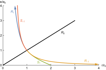
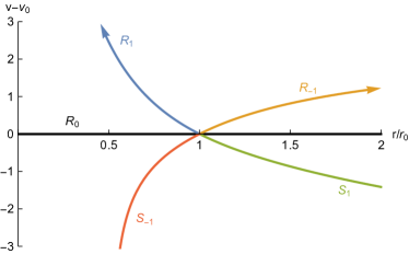
Figure 6: Integral curves for hard-point particles. (a) Internal energy in dependence of stretch for rarefaction and shock curves, see Eqs. (4.6), (4.7) and (4.12), respectively. The black line is the identity function, and the red curve S1subscript𝑆1S_{-1} diverges at r/r0=1/2𝑟subscript𝑟012r/r_{0}=1/2. (b) Velocity in dependence of stretch, see Eqs. (4.8) and (4.13), for m=1𝑚1m=1 and e0=1subscript𝑒01e_{0}=1.

Fig. 6a displays the internal energy in dependence of the stretch, both for the rarefaction and shock curves, denoting by Risubscript𝑅𝑖R_{i} the i𝑖i-th rarefaction curve and by Sisubscript𝑆𝑖S_{i} the i𝑖i-th shock curve. Analogously, Fig. 6b displays the change of velocity in dependence of the stretch. These figures should be compared with Fig. 1. Considering only rarefactions and shocks, the solution to both Riemann problems are qualitatively the same. The contact discontinuity is merely an independent additional feature.

4.3 Entropy

The entropy (3.18) for the hard-point particles is

Shp(r,e)=log(r)+12log(e),subscript𝑆hp𝑟𝑒𝑟12𝑒S_{\text{hp}}(r,e)=\log(r)+\tfrac{1}{2}\log(e), (4.18)

up to a constant shift by 32+12log(4πm)32124𝜋𝑚\tfrac{3}{2}+\tfrac{1}{2}\log(4\pi m). For a jump along a shock curve with speed λ𝜆\lambda, the entropy admissibility condition tS(u)0subscript𝑡𝑆𝑢0\partial_{t}S(\vec{u})\geq 0 becomes

λ(S(r1,e1)S(r0,e0))0,𝜆𝑆subscript𝑟1subscript𝑒1𝑆subscript𝑟0subscript𝑒00\lambda\big{(}S(r_{1},e_{1})-S(r_{0},e_{0})\big{)}\leq 0, (4.19)

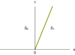
compare to Eq. (47) in [13] with opposite sign. We follow the physics convention of a concave entropy function, while [13] prefers a convex function. In other words, at a shock a region with higher entropy invades a region with lower entropy. Fig. 7 schematically visualizes the time evolution of the entropy across a shock with speed λ>0𝜆0\lambda>0.

Refer to caption
(a) shock x𝑥x-t𝑡t profile
Refer to caption
(b) entropy at t=0𝑡0t=0
Refer to caption
(c) entropy at t>0𝑡0t>0
Figure 7: Schematic illustration of a shock curve with speed λ>0𝜆0\lambda>0 and corresponding time evolution of the entropy.

4.4 Molecular dynamics

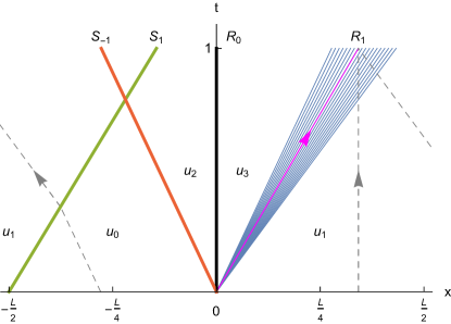
For a molecular dynamics simulation we use a box of size L𝐿L with periodic boundary conditions, for which we adopt the domain [L2,L21]𝐿2𝐿21[-\frac{L}{2},\frac{L}{2}-1]. Imposing domain-wall initial conditions as u0|u1conditionalsubscript𝑢0subscript𝑢1\vec{u}_{0}|\vec{u}_{1} at the origin implies that somewhere else one has the reversed initial condition u1|u0conditionalsubscript𝑢1subscript𝑢0\vec{u}_{1}|\vec{u}_{0}. We call this the periodic Riemann problem. The Riemann problem centered at 00 is of key interest. But numerically we automatically realize two distinct Riemann problems. The longest time of simulation is limited by collisions between the two solution branches. A conventional choice for the masses is m=2𝑚2m=2, corresponding to alternating masses with m0=1subscript𝑚01m_{0}=1 and m1=3subscript𝑚13m_{1}=3. As in [20], we prescribed u1=(r1,v1,𝔢1)=(1,0,1)subscript𝑢1subscript𝑟1subscript𝑣1subscript𝔢1101\vec{u}_{1}=(r_{1},v_{1},\mathfrak{e}_{1})=(1,0,1) and determine the entries of u0subscript𝑢0\vec{u}_{0} such that the rarefaction waves and shocks as shown in Fig. 8 arise. In [20] the goal was to have a wide rarefaction wave. Here we explain in detail how the solution of the periodic Riemann problem is constructed.
Refer to caption
Figure 8: Visualization of the theoretically predicted rarefaction and shock curves for a system of size L𝐿L with periodic boundary conditions and domain-wall initial conditions. The largest time corresponds to L/4𝐿4L/4.

For conciseness, we denote the quotients of the stretches by μ=r1/r3𝜇subscript𝑟1subscript𝑟3\mu=r_{1}/r_{3}, ϕ=r3/r2italic-ϕsubscript𝑟3subscript𝑟2\phi=r_{3}/r_{2}, ω=r2/r0𝜔subscript𝑟2subscript𝑟0\omega=r_{2}/r_{0} and ξ=r0/r1𝜉subscript𝑟0subscript𝑟1\xi=r_{0}/r_{1}. Considering the right rarefaction R1subscript𝑅1R_{1}, condition (4.7) for the internal energy reads e1=μ2e3subscript𝑒1superscript𝜇2subscript𝑒3e_{1}=\mu^{-2}e_{3}, and (4.8) for the velocity

v1=v3+σ6e3/m(1μ1),σ=1.formulae-sequencesubscript𝑣1subscript𝑣3𝜎6subscript𝑒3𝑚1𝜇1𝜎1v_{1}=v_{3}+\sigma\sqrt{6e_{3}/m}\left(\frac{1}{\mu}-1\right),\quad\sigma=1. (4.20)

We can still choose μ𝜇\mu, which we set to μ=45𝜇45\mu=\frac{4}{5} in Fig. 8. Accordingly, r3=54subscript𝑟354r_{3}=\frac{5}{4}, v3=153subscript𝑣3153v_{3}=-\frac{1}{5}\sqrt{3} and e3=1625subscript𝑒31625e_{3}=\frac{16}{25}. It remains to show that u0subscript𝑢0\vec{u}_{0} and u2subscript𝑢2\vec{u}_{2} can be chosen in accordance with Fig. 8. The contact discontinuity R0subscript𝑅0R_{0} at the origin implies that the velocity is conserved, i.e., v2=v3subscript𝑣2subscript𝑣3v_{2}=v_{3}. Furthermore e3/e2=r3/r2=ϕsubscript𝑒3subscript𝑒2subscript𝑟3subscript𝑟2italic-ϕe_{3}/e_{2}=r_{3}/r_{2}=\phi. Considering the shock curve S1subscript𝑆1S_{-1}, according to (4.12),

e2=ω(2ω)2ω1e0,subscript𝑒2𝜔2𝜔2𝜔1subscript𝑒0e_{2}=\frac{\omega(2-\omega)}{2\omega-1}e_{0}, (4.21)

since r2=ωr0subscript𝑟2𝜔subscript𝑟0r_{2}=\omega r_{0} as defined above, and according to (4.13),

v2=v0+6e0/mω12ω1.subscript𝑣2subscript𝑣06subscript𝑒0𝑚𝜔12𝜔1v_{2}=v_{0}+\sqrt{6e_{0}/m}\frac{\omega-1}{\sqrt{2\omega-1}}. (4.22)

Finally, (4.12) for the shock curve S1subscript𝑆1S_{1} implies that

e0=e1ξ(2ξ)2ξ1subscript𝑒0subscript𝑒1𝜉2𝜉2𝜉1e_{0}=e_{1}\frac{\xi(2-\xi)}{2\xi-1} (4.23)

and (4.13) that

v0=v16e1/mξ12ξ1.subscript𝑣0subscript𝑣16subscript𝑒1𝑚𝜉12𝜉1v_{0}=v_{1}-\sqrt{6e_{1}/m}\frac{\xi-1}{\sqrt{2\xi-1}}. (4.24)

In summary, it holds that r1=μr3=μϕr2=μϕωr0=μϕωξr1subscript𝑟1𝜇subscript𝑟3𝜇italic-ϕsubscript𝑟2𝜇italic-ϕ𝜔subscript𝑟0𝜇italic-ϕ𝜔𝜉subscript𝑟1r_{1}=\mu\,r_{3}=\mu\,\phi\,r_{2}=\mu\,\phi\,\omega\,r_{0}=\mu\,\phi\,\omega\,\xi\,r_{1}, i.e.,

μϕωξ=1.𝜇italic-ϕ𝜔𝜉1\mu\,\phi\,\omega\,\xi=1. (4.25)

Similarly,

e1r1=1μ3e3r3=1μ3e2r2=1μ32ω2ω1e0r0=1μ32ω2ω12ξ2ξ1e1r1,subscript𝑒1subscript𝑟11superscript𝜇3subscript𝑒3subscript𝑟31superscript𝜇3subscript𝑒2subscript𝑟21superscript𝜇32𝜔2𝜔1subscript𝑒0subscript𝑟01superscript𝜇32𝜔2𝜔12𝜉2𝜉1subscript𝑒1subscript𝑟1\frac{e_{1}}{r_{1}}=\frac{1}{\mu^{3}}\,\frac{e_{3}}{r_{3}}=\frac{1}{\mu^{3}}\,\frac{e_{2}}{r_{2}}=\frac{1}{\mu^{3}}\,\frac{2-\omega}{2\omega-1}\,\frac{e_{0}}{r_{0}}=\frac{1}{\mu^{3}}\,\frac{2-\omega}{2\omega-1}\,\frac{2-\xi}{2\xi-1}\,\frac{e_{1}}{r_{1}}, (4.26)

which enforces that

1μ32ω2ω12ξ2ξ1=1.1superscript𝜇32𝜔2𝜔12𝜉2𝜉11\frac{1}{\mu^{3}}\,\frac{2-\omega}{2\omega-1}\,\frac{2-\xi}{2\xi-1}=1. (4.27)

The analogous procedure for the velocity leads to

ξ12ξ11ϕμω1ω(2ω)+(1μ)=0.𝜉12𝜉11italic-ϕ𝜇𝜔1𝜔2𝜔1𝜇0-\frac{\xi-1}{\sqrt{2\xi-1}}-\frac{1}{\sqrt{\phi}}\mu\frac{\omega-1}{\sqrt{\omega(2-\omega)}}+(1-\mu)=0. (4.28)

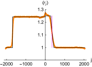
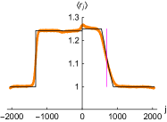
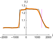
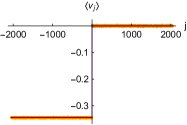
Solving (4.25), (4.27), and (4.28) for ϕitalic-ϕ\phi, ω𝜔\omega and ξ𝜉\xi with the help of a computer algebra program leads to rather lengthy expressions in terms of roots of certain polynomials, which we do not write down explicitly. Instead, we report the numerical values for μ=45𝜇45\mu=\frac{4}{5}, namely ϕ=1.00728italic-ϕ1.00728\phi=1.00728, ω=0.99875𝜔0.99875\omega=0.99875 and ξ=1.2425𝜉1.2425\xi=1.2425. Note that ϕitalic-ϕ\phi and ω𝜔\omega are close to 111. The numerical values for u2subscript𝑢2\vec{u}_{2} are (r2,v2,e2)=(1.241,0.3464,0.63537)subscript𝑟2subscript𝑣2subscript𝑒21.2410.34640.63537(r_{2},v_{2},e_{2})=(1.241,-0.3464,0.63537), and for u0subscript𝑢0\vec{u}_{0} the values read (r0,v0,e0)=(1.2425,0.34469,0.63379)subscript𝑟0subscript𝑣0subscript𝑒01.24250.344690.63379(r_{0},v_{0},e_{0})=(1.2425,-0.34469,0.63379). The shock S1subscript𝑆1S_{-1} is hardly visible, while R1subscript𝑅1R_{1} and S1subscript𝑆1S_{1} are well-developed. The rounding of the edges is presumably a finite size effect. A similar feature is noted in Fig. 4 for the LeRoux lattice gas. An alternative explanation would be rounding because of diffusion. But then this should show also in Fig. 3. To decide larger size systems would have to be simulated.
Refer to caption
(a) stretch, t=0𝑡0t=0
Refer to caption
(b) stretch, t=256𝑡256t=256
Refer to caption
(c) stretch, t=512𝑡512t=512
Refer to caption
(d) stretch, t=1024𝑡1024t=1024
Refer to caption
(e) velocity, t=0𝑡0t=0
Refer to caption
(f) velocity, t=256𝑡256t=256
Refer to caption
(g) velocity, t=512𝑡512t=512
Refer to caption
(h) velocity, t=1024𝑡1024t=1024
Refer to caption
(i) energy, t=0𝑡0t=0
Refer to caption
(j) energy, t=256𝑡256t=256
Refer to caption
(k) energy, t=512𝑡512t=512
Refer to caption
(l) energy, t=1024𝑡1024t=1024
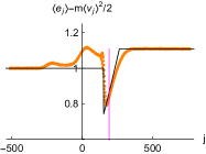
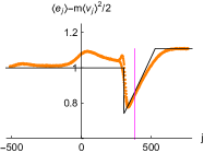
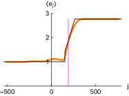
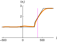
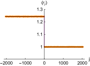
Figure 9: Hard-point particle stretch, velocity and internal energy profiles at various time points, corresponding to the periodic Riemann problem of Fig. 8 with system size L=4096𝐿4096L=4096. The orange dots are molecular dynamics results and the black thin lines show the theoretically predicted profiles.

Fig. 9 shows stretch, velocity, and internal energy profiles obtained by molecular dynamics simulations, after averaging over 106superscript10610^{6} simulation runs with initial states chosen according to u0subscript𝑢0\vec{u}_{0} and u1subscript𝑢1\vec{u}_{1} in Fig. 8. A shock generated through rapid compression is studied in [26].

5 Square-well potential

Hard-point particles are an example of a genuinely nonlinear hyperbolic conservation law. As discussed in [24], in general, one-dimensional fluids do not have such a property and the structure of solutions to the Riemann problem is considerably richer than for hard-points. A similar observation is well known for stochastic dynamics. For a single component genuine nonlinearity corresponds to a convex flux function, which imposes an additional constraint. A two-component stochastic system is studied in [27]. For anharmonic chains we still want to comply with the factorized ideal gas law P(r,e)=2eh(r)𝑃𝑟𝑒2𝑒𝑟P(r,e)=2eh(r), we consider the hard-core potential with core diameter b=0𝑏0b=0 and inward reflection at a𝑎a. This defines the square-well interaction potential (see also [28])

Vsw(x)=0for0xa,Vsw(x)=otherwise.formulae-sequenceformulae-sequencesubscript𝑉sw𝑥0for0𝑥𝑎subscript𝑉sw𝑥otherwiseV_{\mathrm{sw}}(x)=0\quad\mathrm{for}\quad 0\leq x\leq a\,,\quad V_{\mathrm{sw}}(x)=\infty\hskip 4.0pt\mathrm{otherwise}. (5.1)

Since the potential is zero within the well,

e=12β𝑒12𝛽e=\frac{1}{2\beta} (5.2)

and the pressure factorizes as

aβP=h(r/a),𝑎𝛽𝑃𝑟𝑎a\beta P=h(r/a)\,, (5.3)

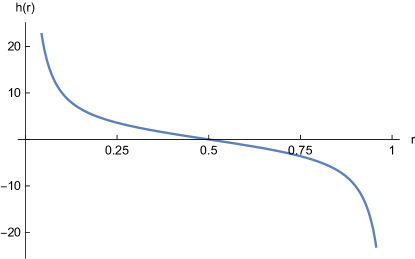
where hh is the inverse function of yy1(ey1)1maps-to𝑦superscript𝑦1superscriptsuperscripte𝑦11y\mapsto y^{-1}-(\mathrm{e}^{y}-1)^{-1}. The unit length can be chosen such that a=1𝑎1a=1, which we adopt in the following. Then (5.3) is rewritten as

P(r,e)=2eh(r).𝑃𝑟𝑒2𝑒𝑟P(r,e)=2eh(r). (5.4)

Hard-point particles are obtained in the limiting case a𝑎a\to\infty, which corresponds to setting h(r)=1/r𝑟1𝑟h(r)=1/r. h(r)𝑟h(r) is visualized in Fig. 10.

Refer to caption
Figure 10: Inverse function to yy1(ey1)1maps-to𝑦superscript𝑦1superscriptsuperscripte𝑦11y\mapsto y^{-1}-(\mathrm{e}^{y}-1)^{-1}, defining the pressure 2eh(r)2𝑒𝑟2eh(r).

Note that derivatives and indefinite integrals can be expressed through hh itself, for example

h(r)=(h(r)214sinh(12h(r))2)1h^{\prime}(r)=-\left(h(r)^{2}-\tfrac{1}{4}\sinh\!\big{(}\tfrac{1}{2}h(r)\big{)}^{-2}\right)^{-1} (5.5)

and

drh(r)=h(r)+h(r)eh(r)1+log(h(r)eh(r)1)1.differential-d𝑟𝑟𝑟𝑟superscripte𝑟1𝑟superscripte𝑟11\int\mathrm{d}r\,h(r)=h(r)+\frac{h(r)}{\mathrm{e}^{h(r)}-1}+\log\!\Big{(}\frac{h(r)}{\mathrm{e}^{h(r)}-1}\Big{)}-1. (5.6)

It is more transparent to keep for a while a general hh, specializing to the square-well potential at the end. The only constraint is h(r)<0superscript𝑟0h^{\prime}(r)<0, ensuring thermodynamic stability. Wendroff [29] discusses a two component model, which in essence corresponds to such a choice upon dropping the contact discontinuity. Inserting (5.4) into (3.14) results in the linearized currents

Ah=(0102meh2vh2mh2veh2(emv2)h2vh)subscript𝐴matrix0102𝑚𝑒superscript2𝑣2𝑚2𝑣𝑒superscript2𝑒𝑚superscript𝑣22𝑣A_{h}=\begin{pmatrix}0&-1&0\\ \tfrac{2}{m}eh^{\prime}&-2vh&\tfrac{2}{m}h\\ 2veh^{\prime}&2\big{(}e-mv^{2}\big{)}h&2vh\end{pmatrix} (5.7)

and the square of the sound speed

ch2=1m(rP+PeP)=1m2e(2h2h).superscriptsubscript𝑐21𝑚subscript𝑟𝑃𝑃subscript𝑒𝑃1𝑚2𝑒2superscript2superscriptc_{h}^{2}=\tfrac{1}{m}(-\partial_{r}P+P\,\partial_{e}P)=\tfrac{1}{m}2e(2h^{2}-h^{\prime}). (5.8)

The right eigenvectors of A𝐴A are

ψ0,h=Z0,h1(2h02eh),ψσ,h=Zσ,h1(σchσ2eh+mvch).formulae-sequencesubscript𝜓0superscriptsubscript𝑍01matrix202𝑒superscriptsubscript𝜓𝜎superscriptsubscript𝑍𝜎1matrix𝜎subscript𝑐𝜎2𝑒𝑚𝑣subscript𝑐\psi_{0,h}=Z_{0,h}^{-1}\begin{pmatrix}2h\\ 0\\ -2eh^{\prime}\end{pmatrix},\qquad\psi_{\sigma,h}=Z_{\sigma,h}^{-1}\begin{pmatrix}-\sigma\\ c_{h}\\ \sigma 2eh+mvc_{h}\end{pmatrix}. (5.9)

The gradient of σch𝜎subscript𝑐\sigma c_{h} along trajectories of the vector field ψσ,hsubscript𝜓𝜎\psi_{\sigma,h} for σ=±1𝜎plus-or-minus1\sigma=\pm 1, i.e., (3.30) for the special case (5.4), is

σψσ,hDch=12e/m4h36hh+h′′2h2h.𝜎subscript𝜓𝜎𝐷subscript𝑐12𝑒𝑚4superscript36superscriptsuperscript′′2superscript2superscript\sigma\psi_{\sigma,h}\cdot Dc_{h}=\tfrac{1}{2}\sqrt{e/m}\,\frac{4h^{3}-6hh^{\prime}+h^{\prime\prime}}{2h^{2}-h^{\prime}}. (5.10)

For the hard-point case, h(r)=1/r𝑟1𝑟h(r)=1/r, this simplifies to (4.10). Note that the right hand side of (5.10) is independent of σ𝜎\sigma, which is achieved by an appropriate choice of the sign of ψσ,hsubscript𝜓𝜎\psi_{\sigma,h}. The square-well potential turns out to violate genuine nonlinearity, since the expression (5.10) changes sign at r=12𝑟12r=\frac{1}{2}. By a suitable choice of hh, presumably one can generate shocks and rarefactions of the same richness as in [29]. Compared to the genuinely nonlinear case the main novel feature is to have a shock at the borderline of a rarefaction wave. For the square-well potential only the case of a left bordering shock is realized. In principle, the shock could also switch to the opposite side, but it cannot lie in the interior of the rarefaction wave.

5.1 Rarefaction curves

Eigenvalue 00:

According to Eq. (3.22)

τ(rv𝔢)=(eP0rP)subscript𝜏matrix𝑟𝑣𝔢matrixsubscript𝑒𝑃0subscript𝑟𝑃\partial_{\tau}\begin{pmatrix}r\\ v\\ \mathfrak{e}\end{pmatrix}=\begin{pmatrix}\partial_{e}P\\ 0\\ -\partial_{r}P\end{pmatrix} (5.11)

with the pressure P(r,e)𝑃𝑟𝑒P(r,e) conserved. Thus from (5.4), it follows that

e(τ)=e0h(r0)h(r(τ)).𝑒𝜏subscript𝑒0subscript𝑟0𝑟𝜏e(\tau)=e_{0}\frac{h(r_{0})}{h(r(\tau))}. (5.12)

Eigenvalue σc𝜎𝑐\sigma c:

According to Eqs. (3.26), (3.27), the stretch obeys r(τ)=r0στ𝑟𝜏subscript𝑟0𝜎𝜏r(\tau)=r_{0}-\sigma\tau and the internal energy τe=σPsubscript𝜏𝑒𝜎𝑃\partial_{\tau}e=\sigma P. Together with (5.4), one obtains

e(τ)=e0exp[2r0r(τ)dρh(ρ)],𝑒𝜏subscript𝑒02superscriptsubscriptsubscript𝑟0𝑟𝜏differential-d𝜌𝜌e(\tau)=e_{0}\exp\!\Big{[}-2\int_{r_{0}}^{r(\tau)}\mathrm{d}\rho\,h(\rho)\Big{]}, (5.13)

which only depends on τ𝜏\tau via r(τ)𝑟𝜏r(\tau). Inserting this relation into the differential equation τv=chsubscript𝜏𝑣subscript𝑐\partial_{\tau}v=c_{h}, the sound speed depending on r(τ)𝑟𝜏r(\tau) and e(τ)𝑒𝜏e(\tau) via (5.8), leads to

τv=σ2e0/mexp[r0r(τ)dρh(ρ)]2h(r(τ))2h(r(τ))r(τ)subscript𝜏𝑣𝜎2subscript𝑒0𝑚superscriptsubscriptsubscript𝑟0𝑟𝜏differential-d𝜌𝜌2superscript𝑟𝜏2superscript𝑟𝜏superscript𝑟𝜏\partial_{\tau}v=-\sigma\,\sqrt{2e_{0}/m}\,\exp\!\Big{[}-\int_{r_{0}}^{r(\tau)}\mathrm{d}\rho\,h(\rho)\Big{]}\sqrt{2h(r(\tau))^{2}-h^{\prime}(r(\tau))}\,r^{\prime}(\tau) (5.14)

and integrates to

v(τ)=v0σ2e0/mr0r(τ)dsexp[r0sdρh(ρ)]2h(s)2h(s).𝑣𝜏subscript𝑣0𝜎2subscript𝑒0𝑚superscriptsubscriptsubscript𝑟0𝑟𝜏differential-d𝑠superscriptsubscriptsubscript𝑟0𝑠differential-d𝜌𝜌2superscript𝑠2superscript𝑠v(\tau)=v_{0}-\sigma\,\sqrt{2e_{0}/m}\int_{r_{0}}^{r(\tau)}\mathrm{d}s\,\exp\!\Big{[}-\int_{r_{0}}^{s}\mathrm{d}\rho\,h(\rho)\Big{]}\sqrt{2h(s)^{2}-h^{\prime}(s)}. (5.15)

5.2 Shock curves

For P𝑃P as in (5.4), Eq. (3.37) leads to

ee0=1h(r0)(rr0)1+h(r)(rr0)𝑒subscript𝑒01subscript𝑟0𝑟subscript𝑟01𝑟𝑟subscript𝑟0\frac{e}{e_{0}}=\frac{1-h(r_{0})(r-r_{0})}{1+h(r)(r-r_{0})} (5.16)

for rr0+1/h(r0)𝑟subscript𝑟01subscript𝑟0r\leq r_{0}+1/h(r_{0}) if h(r0)>0subscript𝑟00h(r_{0})>0 and rr0+1/h(r0)𝑟subscript𝑟01subscript𝑟0r\geq r_{0}+1/h(r_{0}) if h(r0)<0subscript𝑟00h(r_{0})<0. The condition (3.38) leads to

v=v0σsign(rr0)2e0/m(rr0)(h(r)e/e0h(r0)).𝑣subscript𝑣0𝜎sign𝑟subscript𝑟02subscript𝑒0𝑚𝑟subscript𝑟0𝑟𝑒subscript𝑒0subscript𝑟0v=v_{0}-\sigma\,\mathrm{sign}(r-r_{0})\sqrt{2e_{0}/m}\,\sqrt{-(r-r_{0})\big{(}h(r)e/e_{0}-h(r_{0})\big{)}}. (5.17)

For the hard-point particles with h(r)=1/r𝑟1𝑟h(r)=1/r, Eq. (5.17) simplifies to the expression (4.13). Inserting (5.17) into (3.35) results in the shock speed

λh=σ2e0/mh(r)e/e0h(r0)rr0.subscript𝜆𝜎2subscript𝑒0𝑚𝑟𝑒subscript𝑒0subscript𝑟0𝑟subscript𝑟0\lambda_{h}=\sigma\sqrt{2e_{0}/m}\sqrt{-\frac{h(r)e/e_{0}-h(r_{0})}{r-r_{0}}}. (5.18)

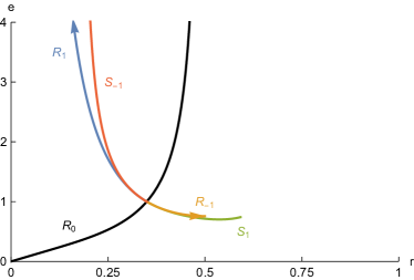
For the square-well potential Fig. 11a visualizes an integral curve of the internal energy in dependence of the stretch, both for the rarefaction and shock curves. Analogously, Fig. 11b visualizes the velocity in dependence of the stretch.
Refer to caption
(a) energy in dependence of stretch
Refer to caption
(b) velocity in dependence of stretch
Figure 11: Integral curves for the square-well potential (5.1) with m=1𝑚1m=1, r0=0.35subscript𝑟00.35r_{0}=0.35, e0=1subscript𝑒01e_{0}=1. (a) Internal energy in dependence of stretch for the rarefaction and shock curves, according to Eqs. (5.12), (5.13) and (5.16), respectively. (b) Velocity in dependence of stretch, see Eqs. (5.15) and (5.17).
Refer to caption
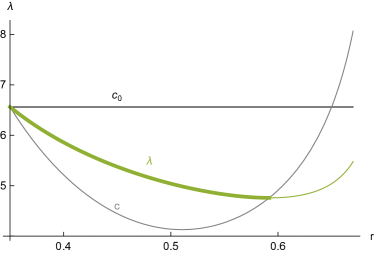
Figure 12: Illustration of the Lax admissibility condition ch,0λhchsubscript𝑐0subscript𝜆subscript𝑐c_{h,0}\geq\lambda_{h}\geq c_{h} for the square-well potential with m=1𝑚1m=1, r0=0.35subscript𝑟00.35r_{0}=0.35, e0=1subscript𝑒01e_{0}=1. The green curve shows the shock speed (5.18) in dependence of the stretch; the condition only holds within the thick curve segment.

The Lax admissibility condition

σch,0λhσch𝜎subscript𝑐0subscript𝜆𝜎subscript𝑐\sigma c_{h,0}\geq\lambda_{h}\geq\sigma c_{h} (5.19)

can be tested numerically for the square-well h(r)𝑟h(r). Fig. 12 shows an example with r0=0.35subscript𝑟00.35r_{0}=0.35 where the condition is satisfied within an interval r0r0.59subscript𝑟0𝑟0.59r_{0}\leq r\leq 0.59. For larger r𝑟r, the sound speed (evaluated along the shock solution (5.16)) becomes larger than λhsubscript𝜆\lambda_{h}.

Refer to caption
Figure 13: A solution of the Euler equation with square-well interaction potential, where a shock wave is followed immediately by a rarefaction wave.

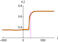
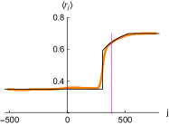
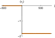
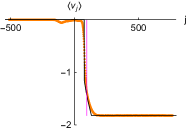
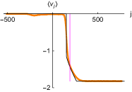
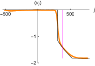
Thus a shock wave is followed immediately by a rarefaction wave, as shown in Fig. 13 with L=18t𝐿18𝑡L=18t. The state to the left of the shock curve is u0=(r0,v0,e0)=(0.35,0,1)subscript𝑢0subscript𝑟0subscript𝑣0subscript𝑒00.3501\vec{u}_{0}=(r_{0},v_{0},e_{0})=(0.35,0,1), and the transition from shock to rarefaction wave appears at r1=0.59subscript𝑟10.59r_{1}=0.59 with u1=(0.59,1.15,0.74)subscript𝑢10.591.150.74\vec{u}_{1}=(0.59,-1.15,0.74). The state u1subscript𝑢1\vec{u}_{1} is connected by a rarefaction wave to u2=(0.7,1.82,1.108)subscript𝑢20.71.821.108\vec{u}_{2}=(0.7,-1.82,1.108).

5.3 Entropy

Specifically for the square-well interaction potential, the entropy equals

Sh(r,e)=rh(r)1+12log(e)log(1+(1r)h(r)),subscript𝑆𝑟𝑒𝑟𝑟112𝑒11𝑟𝑟S_{h}(r,e)=rh(r)-1+\tfrac{1}{2}\log(e)-\log\!\big{(}1+(1-r)h(r)\big{)}, (5.20)

up to a constant shift by 32+12log(4πm)32124𝜋𝑚\tfrac{3}{2}+\tfrac{1}{2}\log(4\pi m). As expected, for the hard-point case h(r)=1/r𝑟1𝑟h(r)=1/r, this expression simplifies to (4.18).

5.4 Molecular dynamics
Refer to caption
(a) stretch, t=0𝑡0t=0
Refer to caption
(b) stretch, t=16𝑡16t=16
Refer to caption
(c) stretch, t=32𝑡32t=32
Refer to caption
(d) stretch, t=64𝑡64t=64
Refer to caption
(e) velocity, t=0𝑡0t=0
Refer to caption
(f) velocity, t=16𝑡16t=16
Refer to caption
(g) velocity, t=32𝑡32t=32
Refer to caption
(h) velocity, t=64𝑡64t=64
Refer to caption
(i) int. energy, t=0𝑡0t=0
Refer to caption
(j) int. energy, t=16𝑡16t=16
Refer to caption
(k) int. energy, t=32𝑡32t=32
Refer to caption
(l) int. energy, t=64𝑡64t=64
Refer to caption
(m) total energy, t=0𝑡0t=0
Refer to caption
(n) total energy, t=16𝑡16t=16
Refer to caption
(o) total energy, t=32𝑡32t=32
Refer to caption
(p) total energy, t=64𝑡64t=64
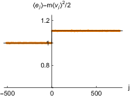
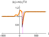
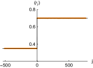
Figure 14: Stretch, velocity, internal energy and total energy profiles for the hard-point particle chain with square-well interaction potential, corresponding to the Riemann problem in Fig. 13 with system size L=4096𝐿4096L=4096. To increase visibility, only a lattice interval around the origin is shown.

Fig. 14 shows stretch, velocity, internal and total energy profiles obtained by molecular dynamics simulations with square-well interaction potential, after averaging over 106superscript10610^{6} simulation runs and initial states chosen according to u0subscript𝑢0\vec{u}_{0} and u2subscript𝑢2\vec{u}_{2} in Fig. 13. The alternating masses are set as m0=1/2subscript𝑚012m_{0}=1/2 and m1=3/2subscript𝑚132m_{1}=3/2, such that the average mass m=1𝑚1m=1. For stretch and velocity the shock followed by a rarefaction wave is well reproduced. For the total energy the shock is not so strong and hence hardly visible. The internal energy is not conserved. Our prediction is based on local equilibrium which apparently is not so accurate close to the shock. The entire system shows still further shocks and rarefaction waves due to periodic boundary conditions. The maximum time t=64𝑡64t=64 in Fig. 14 is chosen prior to their collision with the structure shown in Fig. 13.

6 Fluctuations of the time-integrated current

In a famous contribution Johansson [30] considered the TASEP with 0|1conditional010|1 step initial conditions and particles hopping only to the left. He proved that the time-integrated current along a given ray {x=𝗏t}𝑥𝗏𝑡\{x=\mathsf{v}t\} with |𝗏|<1𝗏1\lvert\mathsf{v}\rvert<1 behaves for large t𝑡t as

Φ(𝗏t,t)c𝗏t+κ𝗏(Γ𝗏t)1/3ξGUE.similar-to-or-equalsΦ𝗏𝑡𝑡subscript𝑐𝗏𝑡subscript𝜅𝗏superscriptsubscriptΓ𝗏𝑡13subscript𝜉GUE\Phi(\mathsf{v}t,t)\simeq c_{\mathsf{v}}t+\kappa_{\mathsf{v}}(\Gamma_{\mathsf{v}}t)^{1/3}\xi_{\mathrm{GUE}}. (6.1)

Following standard conventions, the time scale is denoted by Γ>0Γ0\Gamma>0, in our particular case Γ𝗏subscriptΓ𝗏\Gamma_{\mathsf{v}}. κ=±1𝜅plus-or-minus1\kappa=\pm 1 is the overall sign of the amplitude. The amplitude itself, ξGUEsubscript𝜉GUE\xi_{\mathrm{GUE}}, is a Tracy-Widom GUE distributed random variable, which was originally obtained as the distribution of the largest eigenvalue of a GUE random matrix [31, 32]. In formulas,

(ξGUEs)=det(1Ks)|L2(+)subscript𝜉GUE𝑠evaluated-at1subscript𝐾𝑠superscript𝐿2subscript\mathbb{P}(\xi_{\mathrm{GUE}}\leq s)=\det(1-K_{s})|_{L^{2}(\mathbb{R}_{+})} (6.2)

with the Airy kernel

Ks(x,x)=0dλAi(x+s+λ)Ai(x+s+λ),subscript𝐾𝑠𝑥superscript𝑥superscriptsubscript0differential-d𝜆Ai𝑥𝑠𝜆Aisuperscript𝑥𝑠𝜆K_{s}(x,x^{\prime})=\int_{0}^{\infty}\mathrm{d}\lambda\,\mathrm{Ai}(x+s+\lambda)\mathrm{Ai}(x^{\prime}+s+\lambda), (6.3)

AiAi\mathrm{Ai} denoting the standard Airy function. c𝗏subscript𝑐𝗏c_{\mathsf{v}}, κ𝗏subscript𝜅𝗏\kappa_{\mathsf{v}}, and Γ𝗏subscriptΓ𝗏\Gamma_{\mathsf{v}} are computed, model-dependent parameters, while the exponent 1/3131/3 and ξGUEsubscript𝜉GUE\xi_{\mathrm{GUE}} are universal. Using distinct methods, later the result was extended to a general initial step [33, 34] and also to the ASEP [35].

The Euler equation for the TASEP reads

tux(u(1u))=0,subscript𝑡𝑢subscript𝑥𝑢1𝑢0\partial_{t}u-\partial_{x}\big{(}u(1-u)\big{)}=0, (6.4)

u𝑢u the particle density. To have Tracy-Widom fluctuations the solution to the u|urconditionalsubscript𝑢subscript𝑢ru_{\ell}|u_{\mathrm{r}} Riemann problem for (6.4) has to develop a rarefaction wave and the ray of integration must lie in the interior of the wave. In fact, the rarefaction profile happens to be linear, as for the LeRoux lattice gas. In general the profile will be nonlinear. Still, provided 𝗏𝗏\mathsf{v} is properly chosen, asymptotically the fluctuations of the time-integrated current are expected to have the same probability law as in (6.2). We regard this observation as a strong indication that also the LeRoux lattice gas, even more ambitiously anharmonic chains, has Tracy-Widom statistics for the time-integrated current. There is one immediate difficulty with such a conjecture. The current is a vector. So which linear combination has a statistics governed by ξGUEsubscript𝜉GUE\xi_{\mathrm{GUE}}?

We will first study the fluctuations of time-integrated currents abstractly and then specialize to the LeRoux lattice gas and anharmonic chains with square-well type potential including the hard-point limit.

6.1 Time-integrated currents

To define the time-integrated current, in general, let us start from a conservation law of the form

tu(x,t)+x𝒥(x,t)=0.subscript𝑡𝑢𝑥𝑡subscript𝑥𝒥𝑥𝑡0\partial_{t}u(x,t)+\partial_{x}\mathcal{J}(x,t)=0. (6.5)

Thus, as a property special for one dimension, the vector field (u,𝒥)𝑢𝒥(-u,\mathcal{J}) is curl-free and hence admits a potential, Φ(x,t)Φ𝑥𝑡\Phi(x,t), up to a constant which we fix by Φ(0,0)=0Φ000\Phi(0,0)=0. Φ(x,t)Φ𝑥𝑡\Phi(x,t) is then the current integrated from (0,0)00(0,0) to (x,t)𝑥𝑡(x,t) along an arbitrary integration path. Numerically a convenient choice, to be used later on, is

Φ(x,t)=0tdt𝒥(x,t)0xdxu(x,0),Φ𝑥𝑡superscriptsubscript0𝑡differential-dsuperscript𝑡𝒥𝑥superscript𝑡superscriptsubscript0𝑥differential-dsuperscript𝑥𝑢superscript𝑥0\Phi(x,t)=\int_{0}^{t}\mathrm{d}t^{\prime}\,\mathcal{J}(x,t^{\prime})-\int_{0}^{x}\mathrm{d}x^{\prime}\,u(x^{\prime},0), (6.6)

assuming x>0𝑥0x>0, t>0𝑡0t>0. For a system with n𝑛n components, the same definition applies to each component separately and we set Φ=(Φ1,,Φn)ΦsubscriptΦ1subscriptΦ𝑛\vec{\Phi}=(\Phi_{1},\dots,\Phi_{n}). Clearly, the same argument works also for a spatial lattice with the xsuperscript𝑥x^{\prime}-integration replaced by a lattice sum.

We now consider an n𝑛n component hyperbolic conservation law in the form

tu+x𝗃(u)=0equivalentlytu+A(u)xu=0.formulae-sequencesubscript𝑡𝑢subscript𝑥𝗃𝑢0equivalentlysubscript𝑡𝑢𝐴𝑢subscript𝑥𝑢0\partial_{t}\vec{u}+\partial_{x}\vec{\mathsf{j}}(\vec{u})=0\quad\mathrm{equivalently}\quad\partial_{t}\vec{u}+A(\vec{u})\partial_{x}\vec{u}=0. (6.7)

The linearization matrix A𝐴A has eigenvalues cσsubscript𝑐𝜎c_{\sigma}, left eigenvectors, ψ~σsubscript~𝜓𝜎\tilde{\psi}_{\sigma}, and right eigenvectors, ψσsubscript𝜓𝜎\psi_{\sigma}, σ=1,,n𝜎1𝑛\sigma=1,\dots,n. The eigenvalues are assumed to be non-degenerate. We consider the u|urconditionalsubscript𝑢subscript𝑢r\vec{u}_{\ell}|\vec{u}_{\mathrm{r}} Riemann problem such that its solution contains a rarefaction wave across which u(x)𝑢𝑥\vec{u}(x) increases (or decreases) smoothly for xmin<x<xmaxsubscript𝑥min𝑥subscript𝑥maxx_{\mathrm{min}}<x<x_{\mathrm{max}}. The current is integrated along the ray {x=𝗏t}𝑥𝗏𝑡\{x=\mathsf{v}t\}, which has to lie inside the rarefaction wave, i.e. xmin<𝗏<xmaxsubscript𝑥min𝗏subscript𝑥maxx_{\mathrm{min}}<\mathsf{v}<x_{\mathrm{max}}. The rarefaction wave is associated with a particular eigenvalue, whose label is denoted by σ𝜎\sigma and regarded as fixed in the following. The quantity of interest is the distribution of integrated current Φ(𝗏t,t)Φ𝗏𝑡𝑡\vec{\Phi}(\mathsf{v}t,t). Along {x=𝗏t}𝑥𝗏𝑡\{x=\mathsf{v}t\} the fields take the value u𝗏subscript𝑢𝗏\vec{u}_{\mathsf{v}} and cσ(u𝗏)=𝗏subscript𝑐𝜎subscript𝑢𝗏𝗏c_{\sigma}(\vec{u}_{\mathsf{v}})=\mathsf{v}. Hence, averaging (6.6) in local equilibrium to leading order in t𝑡t,

Φ(𝗏t,t)(𝗃(u𝗏)𝗏u𝗏)t.similar-to-or-equalsΦ𝗏𝑡𝑡𝗃subscript𝑢𝗏𝗏subscript𝑢𝗏𝑡\vec{\Phi}(\mathsf{v}t,t)\simeq\big{(}\,\vec{\mathsf{j}}(\vec{u}_{\mathsf{v}})-\mathsf{v}\vec{u}_{\mathsf{v}}\big{)}t. (6.8)

To access fluctuations we consider a point on {x=𝗏t}𝑥𝗏𝑡\{x=\mathsf{v}t\}, field value u𝗏subscript𝑢𝗏\vec{u}_{\mathsf{v}}, and want to study small fluctuations with shape function f(x)𝑓𝑥\vec{f}(x) which varies on a scale small compared to the variation of the rarefaction wave. Thus we have to linearize (6.7) relative to a homogeneous background u𝗏subscript𝑢𝗏\vec{u}_{\mathsf{v}}. The resulting time evolution is given by

(eAxtf)(x)=σ=1n|ψσψ~σ|f(xcσt),superscripte𝐴subscript𝑥𝑡𝑓𝑥superscriptsubscriptsuperscript𝜎1𝑛ketsubscript𝜓superscript𝜎inner-productsubscript~𝜓superscript𝜎𝑓𝑥subscript𝑐superscript𝜎𝑡(\mathrm{e}^{-A\partial_{x}t}\vec{f}\,)(x)=\sum_{\sigma^{\prime}=1}^{n}|\psi_{\sigma^{\prime}}\rangle\langle\tilde{\psi}_{\sigma^{\prime}}|\vec{f}(x-c_{\sigma^{\prime}}t)\rangle, (6.9)

where |\langle\cdot|\cdot\rangle denotes the scalar product for n𝑛n-vectors and A=A(u𝗏)𝐴𝐴subscript𝑢𝗏A=A(\vec{u}_{\mathsf{v}}). Since cσ(u𝗏)=𝗏subscript𝑐𝜎subscript𝑢𝗏𝗏c_{\sigma}(\vec{u}_{\mathsf{v}})=\mathsf{v}, only the term with σ=σsuperscript𝜎𝜎\sigma^{\prime}=\sigma propagates along the ray 𝗏t𝗏𝑡\mathsf{v}t, while all other components separate from it linearly in time. Hence only ψ~σ|Φ(𝗏t,t)inner-productsubscript~𝜓𝜎Φ𝗏𝑡𝑡\langle\tilde{\psi}_{\sigma}|\vec{\Phi}(\mathsf{v}t,t)\rangle can build up anomalous fluctuations. In case of a single component, the quadratic term is responsible for the t1/3superscript𝑡13t^{1/3} fluctuations. For several components, one first has to transform to normal modes. The strength of the self-coupling is denoted by Gσσσsubscriptsuperscript𝐺𝜎𝜎𝜎G^{\sigma}_{\sigma\sigma}. The slope of the rarefaction profile does not vanish identically, hence classified to be in the KPZ universality class of curved profiles. For it the time scale of the anomalous fluctuations is set by Γσ=|Gσσσ|subscriptΓ𝜎subscriptsuperscript𝐺𝜎𝜎𝜎\Gamma_{\sigma}=\lvert G^{\sigma}_{\sigma\sigma}\rvert. Thus we conjecture that for large t𝑡t

ψ~σ|Φ(𝗏t,t)t(𝗃(u𝗏)𝗏u𝗏)κσ(Γσt)1/3ξGUE.similar-to-or-equalsinner-productsubscript~𝜓𝜎Φ𝗏𝑡𝑡𝑡𝗃subscript𝑢𝗏𝗏subscript𝑢𝗏subscript𝜅𝜎superscriptsubscriptΓ𝜎𝑡13subscript𝜉GUE\big{\langle}\tilde{\psi}_{\sigma}|\vec{\Phi}(\mathsf{v}t,t)-t(\vec{\mathsf{j}}(\vec{u}_{\mathsf{v}})-\mathsf{v}\vec{u}_{\mathsf{v}})\big{\rangle}\simeq\kappa_{\sigma}(\Gamma_{\sigma}t)^{1/3}\xi_{\mathrm{GUE}}. (6.10)

Any linear combination of currents other than in Eq. (6.10) encounters to some part almost independent contributions. Hence, if χ𝜒\chi is not parallel to ψ~σsubscript~𝜓𝜎\tilde{\psi}_{\sigma}, the standard central limit theorem should apply in the form

χ|Φ(𝗏t,t)t(𝗃(u𝗏)𝗏u𝗏)(Γχt)1/2ξG,similar-to-or-equalsinner-product𝜒Φ𝗏𝑡𝑡𝑡𝗃subscript𝑢𝗏𝗏subscript𝑢𝗏superscriptsubscriptΓ𝜒𝑡12subscript𝜉G\big{\langle}\chi|\vec{\Phi}(\mathsf{v}t,t)-t(\vec{\mathsf{j}}(\vec{u}_{\mathsf{v}})-\mathsf{v}\vec{u}_{\mathsf{v}})\big{\rangle}\simeq(\Gamma_{\chi}t)^{1/2}\xi_{\mathrm{G}}, (6.11)

where ξGsubscript𝜉G\xi_{\mathrm{G}} is a standard Gaussian random variable. We have no theoretical prediction for the value of ΓχsubscriptΓ𝜒\Gamma_{\chi}. Of course it has to vanish as χ𝜒\chi tends to ψ~σsubscript~𝜓𝜎\tilde{\psi}_{\sigma}.

As explained in Appendix A, the universal scale factor Γσ=|Gσσσ|subscriptΓ𝜎subscriptsuperscript𝐺𝜎𝜎𝜎\Gamma_{\sigma}=\lvert G^{\sigma}_{\sigma\sigma}\rvert can be computed from thermal averages. There we also establish that

Gσσσ=12σψσDc,σ=±1.formulae-sequencesuperscriptsubscript𝐺𝜎𝜎𝜎12𝜎subscript𝜓𝜎𝐷𝑐𝜎plus-or-minus1G_{\sigma\sigma}^{\sigma}=\tfrac{1}{2}\sigma\psi_{\sigma}\cdot Dc,\quad\sigma=\pm 1. (6.12)

Thus genuine nonlinearity is equivalent to Gσσσsuperscriptsubscript𝐺𝜎𝜎𝜎G_{\sigma\sigma}^{\sigma} having a definite sign for all admissible r𝑟r, e𝑒e.

6.2 Monte-Carlo and molecular dynamics simulations

To shorten notation, we define the projected current components in (6.10), with their asymptotic value subtracted, as

Φσ(t)=ψ~σ|Φ(𝗏t,t)t(𝗃(u𝗏)𝗏u𝗏).subscriptsuperscriptΦ𝜎𝑡inner-productsubscript~𝜓𝜎Φ𝗏𝑡𝑡𝑡𝗃subscript𝑢𝗏𝗏subscript𝑢𝗏\Phi^{\sharp}_{\sigma}(t)=\big{\langle}\tilde{\psi}_{\sigma}|\vec{\Phi}(\mathsf{v}t,t)-t(\vec{\mathsf{j}}(\vec{u}_{\mathsf{v}})-\mathsf{v}\vec{u}_{\mathsf{v}})\big{\rangle}. (6.13)

These are referred to as normal modes of the current.

LeRoux model.

We record the integrated current Φ(𝗏t,t)Φ𝗏𝑡𝑡\vec{\Phi}(\mathsf{v}t,t) for the simulation parameters as in Fig. 3 above, with 𝗏=25𝗏25\mathsf{v}=\frac{2}{5} and 𝗏t𝗏𝑡\mathsf{v}t marked as purple vertical line in Fig. 3. The integrated current is then transformed to normal modes via Eq. (6.13), using the theoretical values for ψ~σsubscript~𝜓𝜎\tilde{\psi}_{\sigma}, u𝗏subscript𝑢𝗏\vec{u}_{\mathsf{v}} and 𝗃(u𝗏)𝗃subscript𝑢𝗏\vec{\mathsf{j}}(\vec{u}_{\mathsf{v}}). The resulting Φσ(t)subscriptsuperscriptΦ𝜎𝑡\Phi^{\sharp}_{\sigma}(t) is shown in Fig. 15 and compared with the theoretical predictions (6.10) and (6.11). The top row shows the standard deviation of Φσ(t)subscriptsuperscriptΦ𝜎𝑡\Phi^{\sharp}_{\sigma}(t) as a function of time, in comparison with σGUE(Γ1t)1/3subscript𝜎GUEsuperscriptsubscriptΓ1𝑡13\sigma_{\mathrm{GUE}}(\Gamma_{1}t)^{1/3} for σ=1𝜎1\sigma=1 and t1/2similar-toabsentsuperscript𝑡12\sim t^{1/2} for σ=1𝜎1\sigma=-1, where σGUEsubscript𝜎GUE\sigma_{\mathrm{GUE}} denotes the standard deviation of the Tracy-Widom distribution. The corresponding probability density functions of Φσ(t)subscriptsuperscriptΦ𝜎𝑡\Phi^{\sharp}_{\sigma}(t) in the bottom row of Fig. 15 are reproduced from [20], and accurately match the predicted Tracy-Widom and Gaussian distributions, respectively. Note that the rescaling uses the theoretical value Γ1=|G111|=0.539subscriptΓ1subscriptsuperscript𝐺1110.539\Gamma_{1}=\lvert G^{1}_{11}\rvert=0.539, see also appendix A.1. However there is still a global shift by 0.180.180.18. Such a shift is familiar from one-component models. The higher cumulants have all relaxed, while the mean is still drifting.
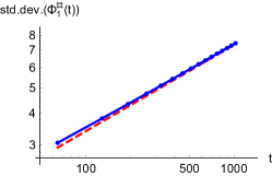
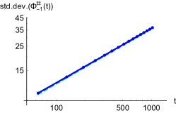
Refer to caption
(a)
Refer to caption
(b)
Refer to caption
(c) (Γ1t)1/3Φ1(t)superscriptsubscriptΓ1𝑡13subscriptsuperscriptΦ1𝑡(\Gamma_{1}t)^{-1/3}\,\Phi^{\sharp}_{1}(t)
Refer to caption
(d) (Γ1t)1/2Φ1(t)superscriptsubscriptΓ1𝑡12subscriptsuperscriptΦ1𝑡(\Gamma_{-1}t)^{-1/2}\,\Phi^{\sharp}_{-1}(t)
Figure 15: (a) Standard deviation of Φ1(t)subscriptsuperscriptΦ1𝑡\Phi^{\sharp}_{1}(t) for the LeRoux model as a function of time, compared with the theoretical prediction σGUE(Γ1t)1/3subscript𝜎GUEsuperscriptsubscriptΓ1𝑡13\sigma_{\mathrm{GUE}}(\Gamma_{1}t)^{1/3}. (b) The standard deviation of Φ1(t)subscriptsuperscriptΦ1𝑡\Phi^{\sharp}_{-1}(t) shows central limit type fluctuations, scaling as t1/2superscript𝑡12t^{1/2} (green dashed). (c) PDF of (Γ1t)1/3Φ1(t)superscriptsubscriptΓ1𝑡13subscriptsuperscriptΦ1𝑡(\Gamma_{1}t)^{-1/3}\,\Phi^{\sharp}_{1}(t) at t=1024𝑡1024t=1024 compared with the Tracy-Widom distribution (red dashed) and (d) PDF of (1.34t)1/2Φ1(t)superscript1.34𝑡12subscriptsuperscriptΦ1𝑡(1.34t)^{-1/2}\,\Phi^{\sharp}_{-1}(t) compared with a normalized Gaussian (green dashed).

Hard-point particles with alternating masses.

Analogous to the LeRoux model, for the hard-point particle chain with alternating masses we integrate stretch, velocity, and energy currents in MD simulations along the purple ray in Figs. 8 and 9, to obtain Φ(𝗏t,t)Φ𝗏𝑡𝑡\vec{\Phi}(\mathsf{v}t,t). For anharmonic chains there are three normal modes Φσ(t)subscriptsuperscriptΦ𝜎𝑡\Phi^{\sharp}_{\sigma}(t), σ=1,0,1𝜎101\sigma=-1,0,1, which we compute from Φ(𝗏t,t)Φ𝗏𝑡𝑡\vec{\Phi}(\mathsf{v}t,t) via (6.13), again using the theoretical values for ψ~σsubscript~𝜓𝜎\tilde{\psi}_{\sigma}, u𝗏subscript𝑢𝗏\vec{u}_{\mathsf{v}} and 𝗃(u𝗏)𝗃subscript𝑢𝗏\vec{\mathsf{j}}(\vec{u}_{\mathsf{v}}). Only the σ=1𝜎1\sigma=1 mode is expected to follow a Tracy-Widom distribution. Fig. 16 shows the simulation results for Φσ(t)subscriptsuperscriptΦ𝜎𝑡\Phi^{\sharp}_{\sigma}(t) in comparison with ξGUEsubscript𝜉GUE\xi_{\mathrm{GUE}} for σ=1𝜎1\sigma=1 and normal distributions for σ=0,1𝜎01\sigma=0,-1. As before, a small correction to the mean values is indicated at the 111-axis labels. The numerical fit uses Γ1=0.86subscriptΓ10.86\Gamma_{1}=0.86, while the theoretical prediction is |G111|=0.559subscriptsuperscript𝐺1110.559\lvert G^{1}_{11}\rvert=0.559.

Refer to caption
(a) std. dev. of Φ1(t)subscriptsuperscriptΦ1𝑡\Phi^{\sharp}_{1}(t)
Refer to caption
(b) std. dev. of Φ0(t)subscriptsuperscriptΦ0𝑡\Phi^{\sharp}_{0}(t)
Refer to caption
(c) std. dev. of Φ1(t)subscriptsuperscriptΦ1𝑡\Phi^{\sharp}_{-1}(t)
Refer to caption
(d) (Γ1t)1/3Φ1(t)superscriptsubscriptΓ1𝑡13subscriptsuperscriptΦ1𝑡(\Gamma_{1}t)^{-1/3}\,\Phi^{\sharp}_{1}(t)
Refer to caption
(e) (Γ0t)1/2Φ0(t)superscriptsubscriptΓ0𝑡12subscriptsuperscriptΦ0𝑡(\Gamma_{0}t)^{-1/2}\,\Phi^{\sharp}_{0}(t)
Refer to caption
(f) (Γ1t)1/2Φ1(t)superscriptsubscriptΓ1𝑡12subscriptsuperscriptΦ1𝑡(\Gamma_{-1}t)^{-1/2}\,\Phi^{\sharp}_{-1}(t)
Refer to caption
(g) (Γ1t)1/3Φ1(t)superscriptsubscriptΓ1𝑡13subscriptsuperscriptΦ1𝑡(\Gamma_{1}t)^{-1/3}\,\Phi^{\sharp}_{1}(t)
Refer to caption
(h) (Γ0t)1/2Φ0(t)superscriptsubscriptΓ0𝑡12subscriptsuperscriptΦ0𝑡(\Gamma_{0}t)^{-1/2}\,\Phi^{\sharp}_{0}(t)
Refer to caption
(i) (Γ1t)1/2Φ1(t)superscriptsubscriptΓ1𝑡12subscriptsuperscriptΦ1𝑡(\Gamma_{-1}t)^{-1/2}\,\Phi^{\sharp}_{-1}(t)
Figure 16: Top row: standard deviation of Φσ(t)subscriptsuperscriptΦ𝜎𝑡\Phi^{\sharp}_{\sigma}(t) as a function of time for the hard-point particle chain with alternating masses. The σ=1𝜎1\sigma=1 component in (a) scales as t1/3superscript𝑡13t^{1/3} (red dashed) and the standard deviations of the σ=0,1𝜎01\sigma=0,-1 components in (b) and (c) scale as t1/2superscript𝑡12t^{1/2} (green dashed). Middle and bottom row: statistical distribution of the rescaled Φ^σ(t)subscriptsuperscript^Φ𝜎𝑡\hat{\Phi}^{\sharp}_{\sigma}(t) at t=1024𝑡1024t=1024. The red dashed curve in (d) and (g) is the predicted Tracy-Widom PDF. The projections for σ=0,1𝜎01\sigma=0,-1 follow a Gaussian distribution (green dashed).

Square-well potential.

To also have an example where genuine nonlinearity is violated, we repeat the analogous analysis for MD simulations with square-well interaction potential, using the parameters as in Figs. 13 and 14. The current is integrated along the ray {x=𝗏t}𝑥𝗏𝑡\{x=\mathsf{v}t\} with 𝗏=6𝗏6\mathsf{v}=6. To avoid collisions due to the periodic boundary conditions, the largest simulation time is relatively short, t=128𝑡128t=128. The results for Φσ(t)subscriptsuperscriptΦ𝜎𝑡\Phi^{\sharp}_{\sigma}(t) are shown in Fig. 17 in comparison with the theoretical predictions. Different from the previous two examples, we show the simulation results without mean value correction. The agreement is slightly less precise as for the alternating masses. One reason could be due to the mentioned short simulation time. Nevertheless, one clearly observes that the mean value of Φ1(t)subscriptsuperscriptΦ1𝑡\Phi^{\sharp}_{1}(t) is close to that of ξGUEsubscript𝜉GUE\xi_{\mathrm{GUE}}, whereas Φσ(t)subscriptsuperscriptΦ𝜎𝑡\Phi^{\sharp}_{\sigma}(t) for σ=0,1𝜎01\sigma=0,-1 are approximately centered around zero, in accordance with the theoretical prediction. The numerically fitted coefficient Γ1=4subscriptΓ14\Gamma_{1}=4, whereas the theoretical prediction is |G111|=2.376subscriptsuperscript𝐺1112.376\lvert G^{1}_{11}\rvert=2.376. The other two numerical coefficients are Γ0=7.6subscriptΓ07.6\Gamma_{0}=7.6 and Γ1=13subscriptΓ113\Gamma_{-1}=13. In Fig. 17, the sign of ψ~1subscript~𝜓1\tilde{\psi}_{1} for the transformation to normal modes is flipped, in accordance with the changing sign in Eq. (5.10).
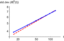
Refer to caption
(a)
Refer to caption
(b)
Refer to caption
(c)
Refer to caption
(d) (Γ1t)1/3Φ1(t)superscriptsubscriptΓ1𝑡13subscriptsuperscriptΦ1𝑡(\Gamma_{1}t)^{-1/3}\,\Phi^{\sharp}_{1}(t)
Refer to caption
(e) (Γ0t)1/2Φ0(t)superscriptsubscriptΓ0𝑡12subscriptsuperscriptΦ0𝑡(\Gamma_{0}t)^{-1/2}\,\Phi^{\sharp}_{0}(t)
Refer to caption
(f) (Γ1t)1/2Φ1(t)superscriptsubscriptΓ1𝑡12subscriptsuperscriptΦ1𝑡(\Gamma_{-1}t)^{-1/2}\,\Phi^{\sharp}_{-1}(t)
Refer to caption
(g) (Γ1t)1/3Φ1(t)superscriptsubscriptΓ1𝑡13subscriptsuperscriptΦ1𝑡(\Gamma_{1}t)^{-1/3}\,\Phi^{\sharp}_{1}(t)
Refer to caption
(h) (Γ0t)1/2Φ0(t)superscriptsubscriptΓ0𝑡12subscriptsuperscriptΦ0𝑡(\Gamma_{0}t)^{-1/2}\,\Phi^{\sharp}_{0}(t)
Refer to caption
(i) (Γ1t)1/2Φ1(t)superscriptsubscriptΓ1𝑡12subscriptsuperscriptΦ1𝑡(\Gamma_{-1}t)^{-1/2}\,\Phi^{\sharp}_{-1}(t)
Figure 17: Top row: standard deviation of Φσ(t)subscriptsuperscriptΦ𝜎𝑡\Phi^{\sharp}_{\sigma}(t) as a function of time for the square-well interaction potential. The σ=1𝜎1\sigma=1 component in (a) scales as t1/3superscript𝑡13t^{1/3} (red dashed), while the standard deviations of the σ=0,1𝜎01\sigma=0,-1 components in (b) and (c) scale almost perfectly as t1/2superscript𝑡12t^{1/2} (green dashed). Middle and bottom row: statistical distribution of the rescaled Φ^σ(t)subscriptsuperscript^Φ𝜎𝑡\hat{\Phi}^{\sharp}_{\sigma}(t) at t=128𝑡128t=128. The red dashed curve in (d) and (g) is the predicted Tracy-Widom PDF. The projections for σ=0,1𝜎01\sigma=0,-1 approximately follow a Gaussian distribution (green dashed).

7 Summary and conclusions

We studied anharmonic chains with nonequilibrium initial conditions, specifically domain-wall. Two rather distinct theoretical predictions have been tested against molecular dynamics simulations.
(i) The validity of the macroscopic Euler equations, which predict flat profiles interrupted by shocks and rarefaction waves. Our system size is moderate, roughly 4000 particles, which we try to compensate by averaging over order 107superscript10710^{7} configurations sampled according to the initial domain-wall state. For times up to the crossing time for a sound wave, the agreement between the solution of the Euler equations and the simulation is fairly accurate. Exceptions are shock fronts, where additional oscillatory structures may appear. Also the borders of rarefaction waves are somewhat rounded.
(ii) We measured currents integrated along a ray in space-time. If this ray lies in a domain with flat profile, one expects t𝑡\sqrt{t} size Gaussian fluctuations. We confirmed such a behavior in a related set-up [28, 36] and did not repeat it here. However, for a ray inside a rarefaction wave we do obtain t1/3superscript𝑡13t^{1/3} size fluctuations with Tracy-Widom GUE distributed random amplitude, provided the current is projected onto the respective left eigenvector. Such a behavior is observed even in case the rarefaction wave does not perfectly approximate the Euler solution.

Turning to stochastic particle dynamics with several components, as to be expected, the precision of the approximation is improved. Our working example is the LeRoux lattice gas. In this model, even strong shocks are realized by the dynamics with a width of a few lattice sites. The Tracy-Widom distribution is confirmed at a precision known for the one-component ASEP.

Acknowledgements.

The work of HS has been supported as a Simons Distinguished Visiting Scholar, when visiting the KITP early 2016. CM acknowledges support from the Alexander von Humboldt Foundation and computing resources of the Leibniz-Rechenzentrum.

Appendix A Coupling matrices

We compute the G𝐺G coupling matrices for the LeRoux model and anharmonic chains, following the derivation in [9].

A.1 LeRoux model

The linearization matrix A𝐴A and its left and right eigenvectors are stated in Eqs. (2.7) and (2.9). The transformation to normal modes is accomplished through the matrix R𝑅R defined by

R=(ψ~1|ψ~1|),R1=(|ψ1|ψ1).R=\begin{pmatrix}\langle\tilde{\psi}_{-1}\rvert\\ \langle\tilde{\psi}_{1}\rvert\end{pmatrix},\quad R^{-1}=\Big{(}\lvert\psi_{-1}\rangle\ \lvert\psi_{1}\rangle\Big{)}. (A.1)

By construction one has

RAR1=diag(c1,c1).𝑅𝐴superscript𝑅1diagsubscript𝑐1subscript𝑐1RAR^{-1}=\mathrm{diag}(c_{-1},c_{1}). (A.2)

As usual, the static susceptibility matrix, C𝐶C, is given by

C=(1|ηj|;1|ηj|1|ηj|;ηj1|ηj|;ηjηj;ηj)=(ρ(1ρ)ρvρv1ρv2).𝐶matrix1subscript𝜂𝑗1subscript𝜂𝑗1subscript𝜂𝑗subscript𝜂𝑗1subscript𝜂𝑗subscript𝜂𝑗subscript𝜂𝑗subscript𝜂𝑗matrix𝜌1𝜌𝜌𝑣𝜌𝑣1𝜌superscript𝑣2C=\begin{pmatrix}\langle 1-\lvert\eta_{j}\rvert;1-\lvert\eta_{j}\rvert\rangle&\langle 1-\lvert\eta_{j}\rvert;\eta_{j}\rangle\\ \langle 1-\lvert\eta_{j}\rvert;\eta_{j}\rangle&\langle\eta_{j};\eta_{j}\rangle\end{pmatrix}=\begin{pmatrix}\rho(1-\rho)&-\rho v\\ -\rho v&1-\rho-v^{2}\\ \end{pmatrix}. (A.3)

In addition we then require

RCRT=𝟙,𝑅𝐶superscript𝑅T1RCR^{\mathrm{T}}=\mathbbm{1}, (A.4)

thereby fixing the normalizations Z~σsubscript~𝑍𝜎\tilde{Z}_{\sigma}, Zσsubscript𝑍𝜎Z_{\sigma} in (2.9) to

Z~σ=2(4ρ(1ρ)+v2(15ρv2)+σv(3ρ+v21)4ρ+v2)1/2,subscript~𝑍𝜎2superscript4𝜌1𝜌superscript𝑣215𝜌superscript𝑣2𝜎𝑣3𝜌superscript𝑣214𝜌superscript𝑣212\tilde{Z}_{\sigma}=\sqrt{2}\left(4\rho(1-\rho)+v^{2}\big{(}1-5\rho-v^{2}\big{)}+\sigma\,v\big{(}3\rho+v^{2}-1\big{)}\sqrt{4\rho+v^{2}}\right)^{1/2}, (A.5)
Zσ=2Z~σ1(4ρv(σ4ρ+v2v)).subscript𝑍𝜎2superscriptsubscript~𝑍𝜎14𝜌𝑣𝜎4𝜌superscript𝑣2𝑣Z_{\sigma}=2\,\tilde{Z}_{\sigma}^{-1}\left(4\rho-v\big{(}\sigma\sqrt{4\rho+v^{2}}-v\big{)}\right). (A.6)

To obtain the nonlinear couplings G𝐺G, in particular G111subscriptsuperscript𝐺111G^{1}_{11}, we first compute the Hessians of the current as second derivatives of 𝗃(u)𝗃𝑢\vec{\mathsf{j}}(\vec{u}),

Hρ=(0110),Hv=(0002).formulae-sequencesuperscript𝐻𝜌matrix0110superscript𝐻𝑣matrix0002H^{\rho}=-\begin{pmatrix}0&1\\ 1&0\end{pmatrix},\qquad H^{v}=-\begin{pmatrix}0&0\\ 0&2\end{pmatrix}. (A.7)

In normal coordinates

ψσ|Hρ|ψτ=ρv(1001)+2ρ4ρ+v2(1ρ12v2)(1001)+v4ρ+v2ρ((1ρ)2v2)(0110)quantum-operator-productsubscript𝜓𝜎superscript𝐻𝜌subscript𝜓𝜏𝜌𝑣matrix10012𝜌4𝜌superscript𝑣21𝜌12superscript𝑣2matrix1001𝑣4𝜌superscript𝑣2𝜌superscript1𝜌2superscript𝑣2matrix0110\langle\psi_{\sigma}|H^{\rho}|\psi_{\tau}\rangle=\rho\,v\begin{pmatrix}1&0\\ 0&1\end{pmatrix}+\frac{2\rho}{\sqrt{4\rho+v^{2}}}\big{(}1-\rho-\tfrac{1}{2}v^{2}\big{)}\begin{pmatrix}-1&0\\ 0&1\end{pmatrix}\\ +\frac{v}{\sqrt{4\rho+v^{2}}}\sqrt{\rho\big{(}(1-\rho)^{2}-v^{2}\big{)}}\begin{pmatrix}0&1\\ 1&0\end{pmatrix} (A.8)

and

ψσ|Hv|ψτ=(1ρv2)(1001)+v4ρ+v2(13ρv2)(1001)24ρ+v2ρ((1ρ)2v2)(0110).quantum-operator-productsubscript𝜓𝜎superscript𝐻𝑣subscript𝜓𝜏1𝜌superscript𝑣2matrix1001𝑣4𝜌superscript𝑣213𝜌superscript𝑣2matrix100124𝜌superscript𝑣2𝜌superscript1𝜌2superscript𝑣2matrix0110\langle\psi_{\sigma}|H^{v}|\psi_{\tau}\rangle=-\big{(}1-\rho-v^{2}\big{)}\begin{pmatrix}1&0\\ 0&1\end{pmatrix}+\frac{v}{\sqrt{4\rho+v^{2}}}\big{(}1-3\rho-v^{2}\big{)}\begin{pmatrix}-1&0\\ 0&1\end{pmatrix}\\ -\frac{2}{\sqrt{4\rho+v^{2}}}\sqrt{\rho\big{(}(1-\rho)^{2}-v^{2}\big{)}}\begin{pmatrix}0&1\\ 1&0\end{pmatrix}. (A.9)

The coupling matrices are thus obtained as

Gσ=12i={ρ,v}RσiRTHiR1=Zσ1(4ρ+v2σv)(12(1σ)0012(1+σ))+Z~σ1ρ((1ρ)2v2)(0110).superscript𝐺𝜎12subscript𝑖𝜌𝑣subscript𝑅𝜎𝑖superscript𝑅Tsuperscript𝐻𝑖superscript𝑅1superscriptsubscript𝑍𝜎14𝜌superscript𝑣2𝜎𝑣matrix121𝜎00121𝜎superscriptsubscript~𝑍𝜎1𝜌superscript1𝜌2superscript𝑣2matrix0110\begin{split}G^{\sigma}&=\tfrac{1}{2}\sum_{i=\{\rho,v\}}R_{\sigma i}\,R^{-\mathrm{T}}H^{i}R^{-1}\\ &=Z_{\sigma}^{-1}\big{(}\sqrt{4\rho+v^{2}}-\sigma v\big{)}\begin{pmatrix}\tfrac{1}{2}(1-\sigma)&0\\ 0&\tfrac{1}{2}(1+\sigma)\end{pmatrix}+\tilde{Z}_{\sigma}^{-1}\sqrt{\rho\big{(}(1-\rho)^{2}-v^{2}\big{)}}\begin{pmatrix}0&1\\ 1&0\end{pmatrix}.\end{split} (A.10)

In particular, comparison with (2.10) shows that

Gσσσ=12ψσDcσ.subscriptsuperscript𝐺𝜎𝜎𝜎12subscript𝜓𝜎𝐷subscript𝑐𝜎G^{\sigma}_{\sigma\sigma}=\tfrac{1}{2}\psi_{\sigma}\cdot Dc_{\sigma}. (A.11)

A.2 General anharmonic chain

To set the scale for the Tracy-Widom distribution, one has to compute G111superscriptsubscript𝐺111G_{11}^{1}. For a general anharmonic chain, in the special case v=0𝑣0v=0, the coupling matrices are derived in [9], a result which should be extended to v0𝑣0v\neq 0. In fact, it turns out that the coupling matrices do not depend on v𝑣v.

Following the notation of [9], the static susceptibility matrix is given by

C=(rj;rjrj;vjrj;ejrj;vjvj;vjvj;ejrj;ejvj;ejej;ej)=(y;y0y;V01/(mβ)v/βy;Vv/β12β2+mv2β1+V;V).𝐶matrixsubscript𝑟𝑗subscript𝑟𝑗subscript𝑟𝑗subscript𝑣𝑗subscript𝑟𝑗subscript𝑒𝑗subscript𝑟𝑗subscript𝑣𝑗subscript𝑣𝑗subscript𝑣𝑗subscript𝑣𝑗subscript𝑒𝑗subscript𝑟𝑗subscript𝑒𝑗subscript𝑣𝑗subscript𝑒𝑗subscript𝑒𝑗subscript𝑒𝑗matrix𝑦𝑦0𝑦𝑉01𝑚𝛽𝑣𝛽𝑦𝑉𝑣𝛽12superscript𝛽2𝑚superscript𝑣2superscript𝛽1𝑉𝑉C=\begin{pmatrix}\langle r_{j};r_{j}\rangle&\langle r_{j};v_{j}\rangle&\langle r_{j};e_{j}\rangle\\ \langle r_{j};v_{j}\rangle&\langle v_{j};v_{j}\rangle&\langle v_{j};e_{j}\rangle\\ \langle r_{j};e_{j}\rangle&\langle v_{j};e_{j}\rangle&\langle e_{j};e_{j}\rangle\end{pmatrix}=\begin{pmatrix}\langle y;y\rangle&0&\langle y;V\rangle\\ 0&1/(m\beta)&v/\beta\\ \langle y;V\rangle&v/\beta&\frac{1}{2}\beta^{-2}+mv^{2}\beta^{-1}+\langle V;V\rangle\end{pmatrix}. (A.12)

The linearization matrix A𝐴A in (3.14) and its right and left eigenvectors in (3.16) and (3.17), respectively, define the transformation to normal modes via

R=(ψ~1|ψ~0|ψ~1|),R1=(|ψ1|ψ0|ψ1)R=\begin{pmatrix}\langle\tilde{\psi}_{-1}\rvert\\ \langle\tilde{\psi}_{0}\rvert\\ \langle\tilde{\psi}_{1}\rvert\end{pmatrix},\quad R^{-1}=\Big{(}\lvert\psi_{-1}\rangle\ \lvert\psi_{0}\rangle\ \lvert\psi_{1}\rangle\Big{)} (A.13)

such that

RAR1=diag(c,0,c),RCRT=𝟙.formulae-sequence𝑅𝐴superscript𝑅1diag𝑐0𝑐𝑅𝐶superscript𝑅T1RAR^{-1}=\mathrm{diag}(-c,0,c),\quad RCR^{\mathrm{T}}=\mathbbm{1}. (A.14)

To have RR1=𝟙𝑅superscript𝑅11RR^{-1}=\mathbbm{1}, the normalization constants of the eigenvectors must satisfy

Z0Z~0=mc2,ZσZ~σ=2mc2forσ=±1.formulae-sequencesubscript𝑍0subscript~𝑍0𝑚superscript𝑐2formulae-sequencesubscript𝑍𝜎subscript~𝑍𝜎2𝑚superscript𝑐2for𝜎plus-or-minus1Z_{0}\tilde{Z}_{0}=mc^{2},\qquad Z_{\sigma}\tilde{Z}_{\sigma}=2mc^{2}\ \ \text{for}\ \ \sigma=\pm 1. (A.15)

An explicit computation of the diagonal entries of RCRT𝑅𝐶superscript𝑅TRCR^{\mathrm{T}} shows that the velocity terms cancel. Hence the relations

Z~0=mΥc,Z~σ=2m/βcforσ=±1formulae-sequencesubscript~𝑍0𝑚Υ𝑐formulae-sequencesubscript~𝑍𝜎2𝑚𝛽𝑐for𝜎plus-or-minus1\tilde{Z}_{0}=\sqrt{m\Upsilon}\,c,\qquad\tilde{Z}_{\sigma}=\sqrt{2m/\beta}\,c\ \ \text{for}\ \ \sigma=\pm 1 (A.16)

from [9] remain valid in general, where Υ=β(y;yV;Vy;V2)+12β1y;yΥ𝛽𝑦𝑦𝑉𝑉superscript𝑦𝑉212superscript𝛽1𝑦𝑦\Upsilon=\beta\left(\langle y;y\rangle\langle V;V\rangle-\langle y;V\rangle^{2}\right)+\frac{1}{2}\beta^{-1}\langle y;y\rangle.

As in [9], we denote the Hessian matrices of the average current by

Hαβi=uαuβ𝗃isubscriptsuperscript𝐻𝑖𝛼𝛽subscriptsubscript𝑢𝛼subscriptsubscript𝑢𝛽subscript𝗃𝑖H^{i}_{\alpha\beta}=\partial_{u_{\alpha}}\partial_{u_{\beta}}\,\mathsf{j}_{i} (A.17)

with the conserved fields u=(r,v,𝔢)𝑢𝑟𝑣𝔢\vec{u}=(r,v,\mathfrak{e}) and the current vector defined in (3.10). The coupling matrices are then given by

Gσ=12i=13RσiRTHiR1superscript𝐺𝜎12superscriptsubscript𝑖13subscript𝑅𝜎𝑖superscript𝑅Tsuperscript𝐻𝑖superscript𝑅1G^{\sigma}=\tfrac{1}{2}\sum_{i=1}^{3}R_{\sigma i}\,R^{-\mathrm{T}}H^{i}R^{-1} (A.18)

for σ=1,0,1𝜎101\sigma=-1,0,1. While the Hessian matrices Hisuperscript𝐻𝑖H^{i} depend on v𝑣v, the coupling matrices are actually independent of v𝑣v. Thus using the formulas in [9] one arrives at

G0=12βmΥ(100000001)superscript𝐺012𝛽𝑚Υmatrix100000001G^{0}=\frac{1}{2\beta\sqrt{m\Upsilon}}\begin{pmatrix}-1&0&0\\ 0&0&0\\ 0&0&1\end{pmatrix} (A.19)

and for σ=±1𝜎plus-or-minus1\sigma=\pm 1

Gσ=Pecrc22mβc(101000101)eP2mβ(12(1+σ)000000012(1σ))+Υ22m/βmc2[(rP)2(e2P)2(rP)(reP)(eP)+(r2P)(eP)2](000010000)+Υ2mc[(rP)(ec)(eP)(rc)](010101010).superscript𝐺𝜎𝑃subscript𝑒𝑐subscript𝑟𝑐22𝑚𝛽𝑐matrix101000101subscript𝑒𝑃2𝑚𝛽matrix121𝜎0000000121𝜎Υ22𝑚𝛽𝑚superscript𝑐2delimited-[]superscriptsubscript𝑟𝑃2superscriptsubscript𝑒2𝑃2subscript𝑟𝑃subscript𝑟subscript𝑒𝑃subscript𝑒𝑃superscriptsubscript𝑟2𝑃superscriptsubscript𝑒𝑃2matrix000010000Υ2𝑚𝑐delimited-[]subscript𝑟𝑃subscript𝑒𝑐subscript𝑒𝑃subscript𝑟𝑐matrix010101010\begin{split}G^{\sigma}&=\frac{P\,\partial_{e}c-\partial_{r}c}{2\sqrt{2m\beta}\,c}\begin{pmatrix}1&0&-1\\ 0&0&0\\ -1&0&1\end{pmatrix}-\frac{\partial_{e}P}{\sqrt{2m\beta}}\begin{pmatrix}\frac{1}{2}(1+\sigma)&0&0\\ 0&0&0\\ 0&0&\frac{1}{2}(1-\sigma)\end{pmatrix}\\ &\quad+\frac{\Upsilon}{2\sqrt{2m/\beta}\,mc^{2}}\left[(\partial_{r}P)^{2}(\partial_{e}^{2}P)-2(\partial_{r}P)(\partial_{r}\partial_{e}P)(\partial_{e}P)+(\partial_{r}^{2}P)(\partial_{e}P)^{2}\right]\begin{pmatrix}0&0&0\\ 0&1&0\\ 0&0&0\end{pmatrix}\\ &\quad+\frac{\sqrt{\Upsilon}}{2\sqrt{m}\,c}\left[(\partial_{r}P)(\partial_{e}c)-(\partial_{e}P)(\partial_{r}c)\right]\begin{pmatrix}0&1&0\\ 1&0&-1\\ 0&-1&0\end{pmatrix}.\end{split} (A.20)

The relation (6.12) follows by using on both sides the expressions provided above.

Note that the signs of some entries in Gσsuperscript𝐺𝜎G^{\sigma} are flipped compared to [9], which is due to different sign conventions for the eigenvectors of A𝐴A.

A.3 Hard-point and square-well potential

The coupling constants for these models have been discussed already in Appendix A of [28]. For completeness, here we adapt to the current sign convention for the eigenvectors and using the velocity (instead of momentum) as field variable. The linearization matrix A𝐴A and its right eigenvectors are stated in Eqs. (5.7) and (5.9). The corresponding left eigenvectors of A𝐴A are

ψ~0,h=Z~0,h1(2ehmv1),ψ~σ,h=Z~σ,h1(2eσhm(ch2σvh)2σh).formulae-sequencesubscript~𝜓0superscriptsubscript~𝑍01matrix2𝑒𝑚𝑣1subscript~𝜓𝜎superscriptsubscript~𝑍𝜎1matrix2𝑒𝜎superscript𝑚subscript𝑐2𝜎𝑣2𝜎\tilde{\psi}_{0,h}=\tilde{Z}_{0,h}^{-1}\begin{pmatrix}2eh\\ -mv\\ 1\end{pmatrix},\qquad\tilde{\psi}_{\sigma,h}=\tilde{Z}_{\sigma,h}^{-1}\begin{pmatrix}2e\sigma h^{\prime}\\ m(c_{h}-2\sigma vh)\\ 2\sigma h\end{pmatrix}. (A.21)

Since the interaction potential is either zero or infinite, Υh=12β1y;y=e/hsubscriptΥ12superscript𝛽1𝑦𝑦𝑒superscript\Upsilon_{h}=\frac{1}{2}\beta^{-1}\langle y;y\rangle=-e/h^{\prime}, and the normalization constants in (A.16) become

Z~0,h=mech/h,Z~σ,h=2mech.formulae-sequencesubscript~𝑍0𝑚𝑒subscript𝑐superscriptsubscript~𝑍𝜎2𝑚𝑒subscript𝑐\tilde{Z}_{0,h}=\sqrt{me}\,c_{h}/\sqrt{-h^{\prime}},\qquad\tilde{Z}_{\sigma,h}=2\sqrt{me}\,c_{h}\,. (A.22)

Specializing (A.19) and (A.20) to the square-well interaction potential leads to the coupling matrices

Gh0=he/m(100000001)superscriptsubscript𝐺0superscript𝑒𝑚matrix100000001G_{h}^{0}=\sqrt{-h^{\prime}\,e/m}\begin{pmatrix}-1&0&0\\ 0&0&0\\ 0&0&1\end{pmatrix} (A.23)

and for σ=±1𝜎plus-or-minus1\sigma=\pm 1

Ghσ=12e/m[12(2h2h)(a3a1a3a1a2a1a3a1a3)4h(12(1+σ)000000012(1σ))]superscriptsubscript𝐺𝜎12𝑒𝑚delimited-[]122superscript2superscriptmatrixsubscript𝑎3subscript𝑎1subscript𝑎3subscript𝑎1subscript𝑎2subscript𝑎1subscript𝑎3subscript𝑎1subscript𝑎34matrix121𝜎0000000121𝜎G_{h}^{\sigma}=\frac{1}{2}\sqrt{e/m}\left[\frac{1}{2(2h^{2}-h^{\prime})}\begin{pmatrix}a_{3}&a_{1}&-a_{3}\\ a_{1}&a_{2}&-a_{1}\\ -a_{3}&-a_{1}&a_{3}\end{pmatrix}-4h\begin{pmatrix}\frac{1}{2}(1+\sigma)&0&0\\ 0&0&0\\ 0&0&\frac{1}{2}(1-\sigma)\end{pmatrix}\right] (A.24)

with

a1=2(h)1/2(hh′′h22h2h),a2=4h(h)1(hh′′2h2),a3=4h36hh+h′′.formulae-sequencesubscript𝑎12superscriptsuperscript12superscript′′superscript22superscript2superscriptformulae-sequencesubscript𝑎24superscriptsuperscript1superscript′′2superscript2subscript𝑎34superscript36superscriptsuperscript′′\begin{split}a_{1}&=2(-h^{\prime})^{-1/2}\big{(}hh^{\prime\prime}-h^{\prime 2}-2h^{2}h^{\prime}\big{)},\\ a_{2}&=4h(-h^{\prime})^{-1}\big{(}hh^{\prime\prime}-2h^{\prime 2}\big{)},\\ a_{3}&=4h^{3}-6hh^{\prime}+h^{\prime\prime}.\end{split} (A.25)

As above, the signs of some entries in Ghσsuperscriptsubscript𝐺𝜎G_{h}^{\sigma} are flipped compared to [28], due to different sign conventions for the eigenvectors of A𝐴A.

References