BFKL evolution and the growth with energy of exclusive and photo-production cross-sections
Abstract
We investigate whether the Balitsky-Fadin-Kuraev-Lipatov (BFKL) low evolution equation is capable to describe the energy dependence of the exclusive photo-production cross-section of vector mesons and on protons. Such cross-sections have been measured by both HERA experiments H1 and ZEUS in electron-proton collisions and by LHC experiments ALICE, CMS and LHCb in ultra-peripheral proton-proton and ultra-peripheral proton-lead collisions. Our approach provides a perturbative description of the rise with energy and relies only on a fit of the initial transverse momentum profile of the proton impact factor, which can be extracted from BFKL fits to inclusive HERA data. We find that BFKL evolution is capable to provide a very good description of the energy dependence of the current data set, while the available fits of the proton impact factor require an adjustment in the overall normalization.
1 Introduction
The Large Hadron Collider (LHC) provides due to its large center of
mass energy a unique opportunity to explore the high energy limit of
Quantum Chromodynamics (QCD). In the presence of a hard scale the
theoretical description of the latter is based on the
Balitsky-Fadin-Kuraev-Lipatov (BFKL) evolution equation [1],
currently known up to next-to-leading order (NLO) [2]
in the strong coupling constant . The bulk of searches for
BFKL dynamics at the LHC concentrates on the analysis of
correlations in azimuthal angels of jets, with the most prominent
example the angular decorrelation of a pair of forward-backward or
Mueller-Navelet jets. Data collected for such angular correlations
during the TeV run provide currently first
phenomenological evidence for BFKL dynamics at the LHC
[3]. More recent attempts on the theory side
include now also the study of angular correlations of up to 4 jets,
which are expected to provide further inside into BFKL dynamics
and the realization of so-called Multi-Regge-Kinematics at the LHC
[4].
The study of angular decorrelation is very attractive from a theory
point of view, since the resulting perturbative description is very
stable and only weakly affected by soft and collinear radiative
corrections. At the same time such angular decorrelations allow only
to probe components of the BFKL kernel associated with non-zero
conformal spin, . The exploration of
components is of interest in
its own right and further allows already to test the calculational
framework of high-energy factorization, which underlies the formulation
of BFKL evolution. On the other hand these studies do not allow to address one of the
central questions of the QCD high energy limit, namely the growth of
perturbative cross-sections with energy. The latter corresponds to the
so-called ‘hard’ Pomeron and is governed by the the conformal spin
zero component of the BFKL kernel.
Unlike the terms, the component is strongly affected
by large (anti-) collinear logarithms which need to be
resummed. Building on [5, 6], such a
resummed NLO BFKL kernel has been constructed in
[7, 8], and employed for a fit
to proton structure functions measured in inclusive Deep Inelastic
Scattering (DIS) at HERA. These results have then been subsequently
used to extract an unintegrated gluon density and to provide
predictions for rapidity and transverse momentum distributions of
forward -jets at the LHC in [9]. In the
following we will study the cross-section for exclusive
photo-production of vector mesons and on a
proton. In particular we are interested on a description of the rise
with center-of-mass energy of the cross-section
(), combining measurements at HERA and the LHC.
At the LHC the cross-sections for the process can
be extracted from ultra-peripheral proton-proton () and
proton-lead () collisions, which allow to test the gluon
distribution in the proton down to very small values of the proton
momentum fraction . For this processes the mass
of the heavy quarks, i.e. charm () and bottom
(), provide the hard mass-scale which allows for a
description within perturbative QCD.
Currently there exist various studies of the data collected during the
TeV run
[10, 11, 12, 13, 14, 15, 16, 17],
see also [18, 19]. In following we focus
on the question whether perturbative BFKL evolution is capable to
describe the rise of the cross-section with energy
i.e. we investigate whether the observed rise can be described
purely perturbatively, avoiding both the use of a fitted
dependence as well as ideas related to gluon saturation. While our
description involves necessarily also a fit of initial conditions to
data, this fit is restricted to the transverse momentum distribution
inside the proton, which has been determined in the analysis of HERA
data in [7, 8]. The
-dependence arises on the other hand due to a solution of the NLO
BFKL equation with collinear improvements, combined with an optimal
renormalization
scale setting.
The outline of this paper is as follows: In Sec. 2 we present the theoretical framework of our study, including a short review of the unintegrated BFKL gluon density of [9] and a determination of the vector meson photo-production impact factor. In Sec. 3 we present the numerical results of our study, including a comparison to data while we present in Sec. 4 our conclusions and an outlook on future work. Two integrals needed for the derivation of the impact factor are collected in the Appendix.
2 Vector meson production in the high energy limit
In the following we describe the framework on which our study is based on. We study the process
| (1) |
where while denotes a quasi-real photon with virtuality ; is the squared center-of-mass energy of the collision. Neglecting proton mass effects, i.e. working in the limit , the following Sudakov decomposition holds for the final state momenta in the high energy limit ,
| (2) |
with and for a generic momentum . With the momentum transfer , the differential cross-section for the exclusive production of a vector meson can be written in the following form
| (3) |
where denotes the scattering amplitude for the reaction for color singlet exchange in the -channel, with an overall factor already extracted.
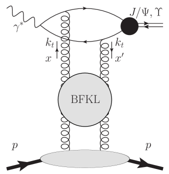
Within high energy factorization i.e. discarding terms
, this scattering amplitude can be written as a
convolution in transverse momentum space of the universal BFKL
Green’s-function, which achieves a resummation of high energy
logarithms to all orders in the strong coupling constant
, and two process-dependent impact factors which describe
the coupling of the Green’s function to external states, see
Fig. 1. In the present case, one of the impact
factors describes the transition and is characterized
by the heavy quark mass and respectively, which provide
the hard scale of the process. The second impact factor, which describes
the transition is of non-perturbative origin; it
needs to be modeled with free parameters to be fixed by a
fit to data.
In the high energy limit , this scattering amplitude is dominated by its imaginary part, , with the real part suppressed by powers of . Limiting ourselves for the moment to the dominant imaginary part we find that for the case of zero momentum transfer, , the non-perturbative proton impact factor coincides for this process with the corresponding proton impact factor found in fits to Deep-Inelastic Scattering data. Such a fit of the forward proton impact factor has been performed in [7, 8] which can be therefore used for phenomenological studies of vector meson production.
2.1 The NLO collinear improved BFKL unintegrated gluon density
In [7, 8] the following model has been used for the proton impact factor
| (4) |
The model introduces 2 free parameters plus an overall normalization factor and provides a Poisson-distribution peaked at .
| virt. photon impact factor | /GeV | |||
|---|---|---|---|---|
| fit 1 | leading order (LO) | |||
| fit 2 | LO with kinematic improvements |
Depending on the precise form of the virtual photon impact factor, two
sets of parameters have been determined, which are summarized in
Tab. 1, where for the second fit the leading order virtual
photon impact factor has been supplemented with DGLAP inspired
kinematic corrections [20]; both
fits have been performed for mass-less flavors.
In [9] the results of this fit have been used to introduce a NLL BFKL unintegrated gluon density as the following convolution of proton impact factor and BFKL Green’s function
| (5) |
In Mellin space conjugate to transverse momentum space this unintegrated gluon density can be written as
| (6) |
where is a characteristic hard scale of the process which in the case of the DIS fit has been identified with the virtuality of the photon and is a corresponding scale which enters the running coupling constant (see also the discussion below); in the DIS analysis and both scales have been identified with the virtuality of the scattering photon. is finally an operator in space and defined as
| (7) |
where with the number of colors and is the next-to-leading logarithmic (NLL) BFKL kernel after collinear improvements; in addition large terms proportional to the first coefficient of the QCD beta function, have been resumed through employing a Brodsky-Lepage-Mackenzie (BLM) optimal scale setting scheme [21]. The NLL kernel with collinear improvements reads
| (8) |
with the leading-order BFKL eigenvalue,
| (9) |
We note that the last term in the second line of Eq. (2.1) was not present in the final results of [7, 8] and [9], but can be easily derived from an intermediate result provided in [7]. It has been re-introduced to assess possible uncertainties of the final result due to identifying . The term responsible for the resummation of collinear enhanced terms reads
| (10) |
For details on the derivation of this term we refer to the discussion in [7], see also [5, 6]. Employing BLM optimal scale setting and the momentum space (MOM) physical renormalization scheme based on a symmetric triple gluon vertex [22] with and gauge parameter one obtains the following next-to-leading order BFKL eigenvalue
| (11) | |||||
where , see also the discussion in [23]. The coefficients which enter the collinear resummation term Eq. (2.1) are obtained as the coefficients of the and poles of the NLO eigenvalue. In the case of Eq. (11) one has
| (12) |
Employing BLM optimal scale setting, the running coupling constant becomes dependent on the Mellin-variable and reads
| (13) |
In addition, in order to access the region of small photon virtualities, in [7, 8], a parametrization of the running coupling introduced by Webber in Ref. [24] has been used,
| (14) |
with GeV. At low scales this modified running coupling
is consistent with global data of power corrections to perturbative
observables, while for larger values it coincides with
the conventional perturbative running coupling constant. For further details we refer the interested reader to [7, 8] and references therein.
2.2 The vector meson photo-production impact factor
To use the above unintegrated gluon density for the description of the process , we still require the impact factor for the transition . To the best of our knowledge, such an impact factor is currently not known within the BFKL framework. It is however possible to extract the required quantity from a description based on a factorization of the amplitude in the high energy limit into light-front wave function and and dipole amplitude. In the dilute limit, the factorization into light-front wave function and dipole amplitude becomes equivalent to the factorization into impact factor and unintegrated gluon density and it is therefore possible to recover the required impact factor from these results. Our starting point is the following expression for the imaginary part of the vector meson photo-production scattering amplitude [26, 25]
| (15) |
where is the dipole amplitude and denotes transverse and longitudinal polarization of the virtual photon respectively and . The overlap between the photon and the vector meson light-front wave function reads
| (16) |
where from now on we discard longitudinal photon polarizations since the corresponding wave function overlap is vanishing in the limit in which we are working. To keep our result applicable to the case , we however keep on using the notation , with for real photons. Furthermore , while denotes the flavor of the heavy quark, with charge , , corresponding to and mesons respectively. For the scalar parts of the wave functions , we follow closely [14] and employ the boosted Gaussian wave-functions with the Brodsky-Huang-Lepage prescription [27]. For the ground state vector meson () the scalar function , has the following general form [26, 28],
| (17) |
The free parameters and of this model have been determined in various studies from the normalization condition of the wave function and the decay width of the vector mesons. In the following we use the most recent available values i.e. [14] (for the ) and [16] (for the ) The results are summarized in Tab. 2.
| Meson | / | /GeV | ||||
|---|---|---|---|---|---|---|
In the forward limit , the entire dependence of the integrand on the impact parameter is contained in the dipole amplitude which results into the following inclusive dipole cross-section,
| (18) |
The relation between the latter and an unintegrated gluon density has been worked in [29] and is given by
| (19) |
This expression can then be used to calculate the BFKL impact factor from the light-front wave function overlap Eq. (2.2). In particular we find
| (20) |
In the above expression, and are the mass-scales introduced in Eq. (2.1). The scale of the strong coupling in Eq. (19), (2.2) has been set in accordance with the conventions used in the HERA fit111A precise determination of the scale of this running coupling would require the complete NLO corrections to the impact factor which are currently not available [8]. From Eq. (2.2) we obtain
| (21) |
where is a hypergeometric function of the second kind or Kummer’s function. Some useful integrals in the derivation of this result are summarized in the appendix. Expanding Eq. (2.2) to NLO in , it is straightforward to verify that our result is independent of to NLO accuracy. Furthermore one can verify that the resummed BFKL eigenvalue Eq. (2.1) is furthermore independent of the choice of up to terms .
2.3 Real part, phenomenological corrections and integrated cross-sections
Even though the real part of the scattering amplitude is suppressed by powers of in the high energy limit, it can still provide a sizable correction to the cross-section and should be therefore included. In the high energy limit it is possible to obtain this real part from the imaginary part using dispersion relation. One has
| with | (22) |
Eq. (22) is frequently used in the literature in the study of photo-production of vector mesons. Within our framework we write first the imaginary part of the scattering amplitude as a double Mellin transform
| (23) |
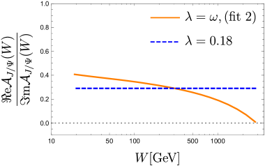
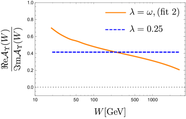
where the -contour runs to the right of all singularities and
, with GeV the proton
mass; note that due to . To determine the
real part we identify with the Mellin variable conjugate to
the , . The complete amplitude is then obtained
through multiplying the integrand of Eq. (2.3)
by a factor . The
Mellin transform w.r.t. is then easily evaluated through
taking residues at the single and double pole at
, while residues at
are subleading in the high energy/low
limit and therefore neglected. As a consequence we obtain – in
contrast to the bulk of phenomenological studies in the literature –
an energy dependent ratio of real and imaginary part, see
Fig. 2 for numerical results. Particular for small
values of , the real part provides a relative large correction, up
to in the case of the and in the case of the
, see also the discussion in [30]. On the
other hand, since this ratio is decreasing with increasing , we
find that this energy-dependent ratio leads to a slow-down of the
growth with energy in the high energy region.
Another phenomenological correction to the cross-section, which is
often included in studies of vector meson photo-production, arises due
to the fact that the proton momentum fractions , of the two
gluons coupling to the transition, can differ, even
though we are working in the forward limit . In
[31] a corresponding corrective factor has been
determined for the case of the conventional (integrated) gluon
distribution, by relating the latter through a Shuvaev transform to
the generalized parton distribution (GPD). Since we are dealing in
the current case with an transverse momentum dependent (unintegrated)
gluon density, such a corrective factor would at best be correct
approximately. Our numerical studies find no significant improvement
in the description of data due to such a factor and we therefore
do not include it in our analysis.
While we calculated so far the differential cross-section at momentum transfer , experimental data which we wish to analyze, are usually given for cross-sections integrated over . It is therefore necessary to model the -dependence and to relate in this way the differential cross-section at to the integrated cross-section. Here we follow the prescription given in [10, 11], who assume an exponential drop-off with , with an energy dependent slope parameter , which can be motivated by Regge theory,
| (24) |
For the numerical values we use GeV-2, GeV and GeV-2 in the case of the , while GeV-2 for production, as proposed in [10, 11]. The total cross-section for vector meson production is therefore obtained as
| (25) |
For the sake of completeness we further provide our final expression for the differential cross-section at . It is given by Eq. (3) for the case with
| (26) |
where .
3 Numerical results and Discussion
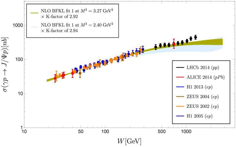
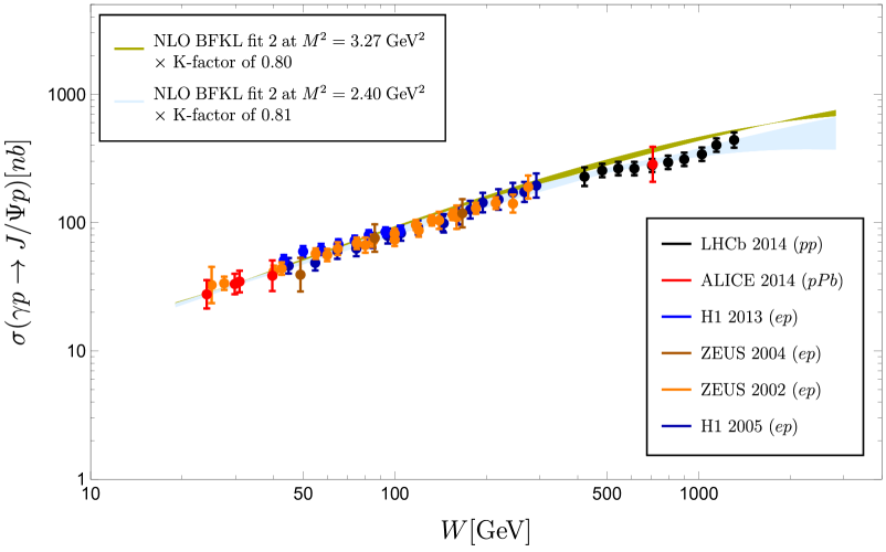
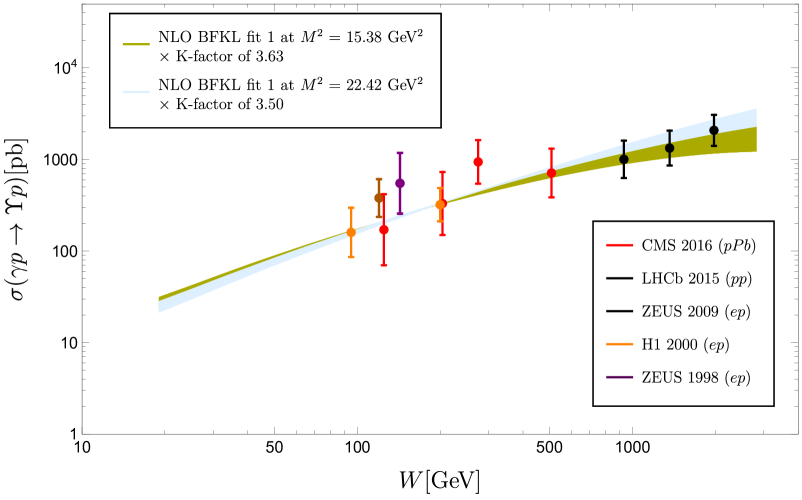
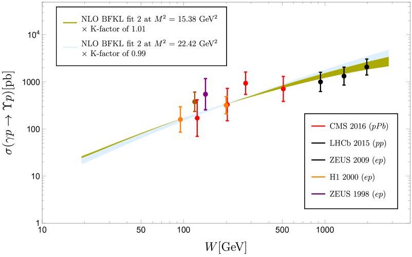
Our results for the -dependence of the total
cross-section are depicted in Fig. 3 ()
and Fig. 4 ()and compared to data
from HERA and LHC experiments. Both fits of free parameters of the
proton impact factor, summarized in Tab. 1, are shown in
the plots. We further show results for two different choices of the
‘hard’ scale of the unintegrated gluon density, i.e. the
photoproduction scale and the scale
, see Tab. 2 for numerical values.
The choice is motivated by the structure of
the impact factor Eq. (2.2), where it cancels the
(-independent part) of the factor and therefore
removes the scale dependence222The impact factor is of course
still dependent on ratios of other scales. This is natural since,
unlike the inclusive DIS impact factor, it is not characterized by a
single hard scale.; we further find that the this choice seems to
minimize the size of the term in
Eq. (2.3). We find that our result is only mildly
dependent on this choice. Since the effective Pomeron intercept
increases with increasing hard scale, see also
[7, 8], the observed rise is
always slightly stronger for the larger of the two scales. We further
identify , while we vary in the
interval to assess the uncertainty associated with
this choice. We find that the result is
rather stable under this variation.
Comparing our results with data we find that the overall normalization
obtained from the combination of BFKL gluon density and
impact factor does – for the majority of cases – not coincide with
measured data. This is in particular true for the BFKL fit 1, where
typical values of necessary K-factors lie in the range . The
BFKL fit 2 requires on the other hand only a small ( for
) or no correction ( for ). In the
current analysis we fix this normalization by the central values of
some arbitrarily picked low energy data points, i.e. low energy
ALICE () and ZEUS () data. While it is possible to
improve further the description through fitting the normalization to
the entire data set, we believe that the current treatment is best
suited to study the description of the -dependence, on which we
focus here.
Turning to the -dependence we find that both fits and both scale
choices allow for an excellent description of data in the case of
-production, see Fig. 4, where fit 2
essentially requires no K-factor. For the data set we find
that fit 2 provides a very good description of the data (with a
-factor of order one), revealing a slight preference for
the photoproduction scale . The BFKL description
based on the fit 1 also allows for a very good description of the
-dependence up to the last 2 LHCb data points, for which the
predicted growth with is too slow. Despite of this slight mismatch
of fit 1 in the case of production, we find that the observed
agreement with data is remarkable. This is in particular true for data
points with GeV which require -evolution beyond the
region constrained by the fit to HERA data and for which the obtained
description directly tests the validity of the present implementation
of NLO BFKL evolution.
While the observed mismatch in the overall normalization is not completely satisfactory, it is somehow expected and – at least for the BFKL fit 2 where the correction is small – easily explained by the limitations of the current framework. In the case of fit 1 a first improvement is obtained if corrections due to (as available for the collinear gluon distribution function as discussed in Sec. 2.3) are included. Nevertheless also these corrections are not capable to account for the complete -factor. For fit 2 one has to take into account that this fit is based on a leading order virtual photon impact factor with kinematic improvements [20], while the currently used impact factor for the transition does not contain such kinematic improvements; in the case of such corrections would also include corrections due to . While the kinematic improvements reduce in the case of DIS studies the magnitude of the impact factors, corrections due to are for the case of vector mesons known to enhance the impact factor, at least in the collinear limit. In the case of fit 2 we therefore expect to a large extend a cancellation of both effects. A second point which applies both to fit 1 and fit 2 is concerned with the treatment of heavy quark masses: while the impact factor Eq. (2.2) obviously depends on the heavy quark mass, the original DIS fits are limited to mass-less flavors. Altogether we believe that it is more than plausible that such effects can account for the observed mismatch in normalization, in particular in the case of fit 2 where the mismatch is rather mild.
4 Outlook and Conclusions
In this work we applied the inclusive BFKL fit of
[8] to the description of exclusive vector
meson photo-production at HERA and the LHC. As a new result we
calculated the impact factor for the transition in the
-Mellin space representation, using earlier result based on
the light-front wave function of vector mesons used in the combination
with color dipole models. Our phenomenological studies show that the
BFKL fits of [8] can provide a very good
description of the center-of-mass energy dependence of the
and cross-sections.
While the BFKL fit 1 requires a relatively large adjustment in the
overall normalization (of order ), the necessary adjustment is
of order one in the case of BFKL fit 2. We stress that the current
analysis uses only a fit of the transverse momentum distribution in
the proton, while the -dependence directly results from NLO BFKL
resummation, together with a resummation of collinearly enhanced terms
within the NLO kernel and a optimal renormalization scale setting for
the scale invariant terms of the NLO BFKL kernel. The study provides
therefore direct evidence for the validity of BFKL
evolution at the LHC.
Despite of the success of the current description, there are a number of directions in which our analysis could and should be re-fined. This implies at first the determination of kinematic corrections to the impact factor for the transition , which might provide an opportunity to improve on the observed mismatch in the overall normalization. To improve the description further, it will be necessary to provide a re-fit of HERA data which takes into account heavy quark masses and possibly now available next-to-leading order corrections to the virtual photon impact factor with massless quarks. On the level of the cross-section this would then further require the determination of corresponding NLO corrections for the impact factor, e.g. using the calculational techniques developed and used in NLO calculations within high energy factorization [43, 44, 45].
Acknowledgments
The authors acknowledge support by CONACyT-Mexico grant number CB-2014-241408. We further would like to thank Laurent Favart for pointing out an erroneous H1 data point in an earlier version of this paper.
Appendix A Integrals used in the calculation of the impact factor
To determine from the BFKL gluon density, it is necessary to calculate
| (27) |
With the individual integrals are not convergent. It is therefore necessary to introduce a a regulator which will set to zero at the end of the calculation (after cancellation of the divergence in Eq. (27)). We obtain
| (28) |
while
| (29) |
and therefore
| (30) |
In a second step we need to integrate over the dipole size . With
| (31) |
this can be done using the following integral:
| (32) |
where is a Hypergeometric function of the second kind or Kummer’s function.
References
- [1] L. N. Lipatov, Sov. J. Nucl. Phys. 23 (1976) 338, E. A. Kuraev, L. N. Lipatov, V. S. Fadin, Phys. Lett. B 60 (1975) 50, Sov. Phys. JETP 44 (1976) 443, Sov. Phys. JETP 45 (1977) 199. I. I. Balitsky, L. N. Lipatov, Sov. J. Nucl. Phys. 28 (1978) 822.
- [2] V. S. Fadin, L. N. Lipatov, Phys. Lett. B 429 (1998) 127, M. Ciafaloni, G. Camici, Phys. Lett. B 430 (1998) 349.
- [3] M. Misiura [CMS Collaboration], Acta Phys. Polon. B 45, no. 7, 1543 (2014); B. Ducloué, L. Szymanowski and S. Wallon, Phys. Rev. Lett. 112 (2014) 082003 [arXiv:1309.3229 [hep-ph]]; F. Caporale, D. Y. Ivanov, B. Murdaca and A. Papa, Eur. Phys. J. C 74 (2014) no.10, 3084 Erratum: [Eur. Phys. J. C 75 (2015) no.11, 535] [arXiv:1407.8431 [hep-ph]].
- [4] F. Caporale, G. Chachamis, B. Murdaca and A. Sabio Vera, Phys. Rev. Lett. 116, no. 1, 012001 (2016) [arXiv:1508.07711 [hep-ph]]; F. Caporale, F. G. Celiberto, G. Chachamis and A. Sabio Vera, Eur. Phys. J. C 76, no. 3, 165 (2016) [arXiv:1512.03364 [hep-ph]]; F. Caporale, F. G. Celiberto, G. Chachamis, D. G. Gomez and A. Sabio Vera, arXiv:1603.07785 [hep-ph]; arXiv:1606.00574 [hep-ph].
- [5] G. P. Salam, JHEP 9807 (1998) 019 [hep-ph/9806482].
- [6] A. Sabio Vera, Nucl. Phys. B 722 (2005) 65 [hep-ph/0505128].
- [7] M. Hentschinski, A. Sabio Vera and C. Salas, Phys. Rev. Lett. 110 (2013) no.4, 041601 [arXiv:1209.1353 [hep-ph]].
- [8] M. Hentschinski, A. Sabio Vera and C. Salas, Phys. Rev. D 87 (2013) no.7, 076005 [arXiv:1301.5283 [hep-ph]].
- [9] G. Chachamis, M. Deàk, M. Hentschinski, G. Rodrigo and A. Sabio Vera, JHEP 1509, 123 (2015) [arXiv:1507.05778 [hep-ph]].
- [10] S. P. Jones, A. D. Martin, M. G. Ryskin and T. Teubner, J. Phys. G 41, 055009 (2014) [arXiv:1312.6795 [hep-ph]].
- [11] S. P. Jones, A. D. Martin, M. G. Ryskin and T. Teubner, JHEP 1311, 085 (2013) [arXiv:1307.7099].
- [12] V. P. Goncalves, L. A. S. Martins and W. K. Sauter, Eur. Phys. J. C 76 (2016) no.2, 97 [arXiv:1511.00494 [hep-ph]].
- [13] R. Fiore, L. Jenkovszky, V. Libov and M. Machado, Theor. Math. Phys. 182, no. 1, 141 (2015) [Teor. Mat. Fiz. 182, no. 1, 171 (2014)] [arXiv:1408.0530 [hep-ph]].
- [14] N. Armesto and A. H. Rezaeian, Phys. Rev. D 90, no. 5, 054003 (2014) [arXiv:1402.4831 [hep-ph]].
- [15] V. P. Goncalves, B. D. Moreira and F. S. Navarra, Phys. Rev. C 90, no. 1, 015203 (2014) [arXiv:1405.6977 [hep-ph]].
- [16] V. P. Goncalves, B. D. Moreira and F. S. Navarra, Phys. Lett. B 742, 172 (2015) [arXiv:1408.1344 [hep-ph]].
- [17] W. Schäfer and A. Szczurek, Phys. Rev. D 76, 094014 (2007) [arXiv:0705.2887 [hep-ph]]; A. Cisek, W. Schäfer and A. Szczurek, JHEP 1504, 159 (2015) [arXiv:1405.2253 [hep-ph]].
- [18] M. S. Costa and M. Djuric, Phys. Rev. D 86, 016009 (2012) [arXiv:1201.1307 [hep-th]]; M. S. Costa, M. Djurić and N. Evans, JHEP 1309 (2013) 084 [arXiv:1307.0009 [hep-ph]].
- [19] V. P. Goncalves and W. K. Sauter, Phys. Rev. D 81, 074028 (2010) [arXiv:0911.5638 [hep-ph]]; Eur. Phys. J. A 47, 117 (2011) [arXiv:1004.1952 [hep-ph]].
- [20] J. Kwiecinski, A. D. Martin and A. M. Stasto, Phys. Rev. D 56, 3991 (1997) [hep-ph/9703445]; A. Bialas, H. Navelet and R. B. Peschanski, Nucl. Phys. B 603, 218 (2001) [hep-ph/0101179].
- [21] S. J. Brodsky, G. P. Lepage and P. B. Mackenzie, Phys. Rev. D 28 (1983) 228.
- [22] W. Celmaster and R. J. Gonsalves, Phys. Rev. D 20 (1979) 1420.
- [23] S. J. Brodsky, V. S. Fadin, V. T. Kim, L. N. Lipatov and G. B. Pivovarov, JETP Lett. 76 (2002) 249 [Pisma Zh. Eksp. Teor. Fiz. 76 (2002) 306] [hep-ph/0207297]; JETP Lett. 70 (1999) 155 [hep-ph/9901229].
- [24] B. R. Webber, JHEP 9810 (1998) 012 [hep-ph/9805484].
- [25] H. Kowalski, L. Motyka and G. Watt, Phys. Rev. D 74, 074016 (2006) [hep-ph/0606272].
- [26] B. E. Cox, J. R. Forshaw and R. Sandapen, JHEP 0906, 034 (2009) [arXiv:0905.0102 [hep-ph]].
- [27] S. J. Brodsky, T. Huang and G. P. Lepage, “The Hadronic Wave Function in Quantum Chromodynamics,” SLAC-PUB-2540.
- [28] J. Nemchik, N. N. Nikolaev and B. G. Zakharov, Phys. Lett. B 341, 228 (1994) [hep-ph/9405355], J. Nemchik, N. N. Nikolaev, E. Predazzi and B. G. Zakharov, Z. Phys. C 75, 71 (1997) [hep-ph/9605231], Z. Phys. C 75, 71 (1997) [hep-ph/9605231].
- [29] K. Kutak and A. M. Stasto, Eur. Phys. J. C 41, 343 (2005) [hep-ph/0408117].
- [30] S. P. Baranov, Phys. Rev. D 76, 034021 (2007).
- [31] A. G. Shuvaev, K. J. Golec-Biernat, A. D. Martin and M. G. Ryskin, Phys. Rev. D 60, 014015 (1999) [hep-ph/9902410].
- [32] S. Chekanov et al. [ZEUS Collaboration], Eur. Phys. J. C 24, 345 (2002) [hep-ex/0201043].
- [33] S. Chekanov et al. [ZEUS Collaboration], Nucl. Phys. B 695, 3 (2004) [hep-ex/0404008].
- [34] C. Alexa et al. [H1 Collaboration], Eur. Phys. J. C 73, no. 6, 2466 (2013) [arXiv:1304.5162 [hep-ex]].
- [35] A. Aktas et al. [H1 Collaboration], Eur. Phys. J. C 46, 585 (2006) [hep-ex/0510016].
- [36] B. B. Abelev et al. [ALICE Collaboration], Phys. Rev. Lett. 113, no. 23, 232504 (2014) [arXiv:1406.7819 [nucl-ex]].
- [37] R. Aaij et al. [LHCb Collaboration], J. Phys. G 40, 045001 (2013) [arXiv:1301.7084 [hep-ex]]; J. Phys. G 41, 055002 (2014) [arXiv:1401.3288 [hep-ex]].
- [38] C. Adloff et al. [H1 Collaboration], Phys. Lett. B 483, 23 (2000) [hep-ex/0003020].
- [39] J. Breitweg et al. [ZEUS Collaboration], Phys. Lett. B 437 (1998) 432 [hep-ex/9807020].
- [40] S. Chekanov et al. [ZEUS Collaboration], Phys. Lett. B 680, 4 (2009) [arXiv:0903.4205 [hep-ex]].
- [41] R. Aaij et al. [LHCb Collaboration], JHEP 1509, 084 (2015) [arXiv:1505.08139 [hep-ex]].
- [42] CMS Collaboration [CMS Collaboration], “Measurement of exclusive Y photoproduction in pPb collisions at ,” CMS-PAS-FSQ-13-009.
- [43] M. Hentschinski and A. Sabio Vera, Phys. Rev. D 85 (2012) 056006 [arXiv:1110.6741 [hep-ph]]; M. Hentschinski, Nucl. Phys. B 859 (2012) 129 [arXiv:1112.4509 [hep-ph]]; G. Chachamis, M. Hentschinski, J. D. Madrigal Martinez and A. Sabio Vera, Nucl. Phys. B 876 (2013) 453 [arXiv:1307.2591 [hep-ph]]; Phys. Rev. D 87 (2013) no.7, 076009 [arXiv:1212.4992]; Nucl. Phys. B 861 (2012) 133 [arXiv:1202.0649 [hep-ph]];
- [44] M. Hentschinski, J. D. Madrigal Martínez, B. Murdaca and A. Sabio Vera, Phys. Lett. B 735 (2014) 168 [arXiv:1404.2937 [hep-ph]]; Nucl. Phys. B 887 (2014) 309 [arXiv:1406.5625 [hep-ph]]; Nucl. Phys. B 889 (2014) 549 [arXiv:1409.6704 [hep-ph]];
- [45] A. Ayala, M. Hentschinski, J. Jalilian-Marian and M. E. Tejeda-Yeomans, arXiv:1604.08526 [hep-ph].