Multiple scattering of polarized light in disordered media exhibiting short-range structural correlations

Abstract

We develop a model based on a multiple scattering theory to describe the diffusion of polarized light in disordered media exhibiting short-range structural correlations. Starting from exact expressions of the average field and the field spatial correlation function, we derive a radiative transfer equation for the polarization-resolved specific intensity that is valid for weak disorder and we solve it analytically in the diffusion limit. A decomposition of the specific intensity in terms of polarization eigenmodes reveals how structural correlations, represented via the standard anisotropic scattering parameter $g$, affect the diffusion of polarized light. More specifically, we find that propagation through each polarization eigenchannel is described by its own transport mean free path that depends on $g$ in a specific and non-trivial way.

I Introduction

Electromagnetic waves propagating in disordered media are progressively scrambled by refractive index fluctuations and, thanks to interference, result into mesoscopic phenomena, such as speckle correlations and weak localization Akkermans and Montambaux (2011); Sheng (2010). Polarization is an essential characteristic of electromagnetic waves that, considering the ubiquity of scattering processes in science, prompted the development of research in statistical optics Goodman (2015); Brosseau (1998) and impacted many applications, from optical imaging in biological tissues Tuchin et al. (2006) to material spectroscopy (e.g., rough surfaces) Maradudin (2007), and radiation transport in turbulent atmospheres Andrews and Phillips (2005); Shirai et al. (2003). Although the topic has experienced numerous developments and outcomes in the past decades, recent studies have revealed that much remains to be explored and understood on the relation between the microscopic structure of scattering media and the polarization properties of the scattered field. In particular, it was found that important information about the morphology of a disordered medium is contained in the three-dimensional (3D) polarized speckles produced in the near-field above its surface Apostol and Dogariu (2003); Carminati (2010); Parigi et al. (2016) and in the spontaneous emission properties of a light source in the bulk Cazé et al. (2010); Sapienza et al. (2011). Similarly, the light scattered by random ensembles of large spheres was shown to exhibit unusual polarization features due to the interplay between the various multipolar scatterer resonances Schmidt et al. (2015).

The fact that light transport is affected by the microscopic structural properties of disordered media is well known. Structural correlations, coming from the finite scatterer size or from the specific morphology of porous materials Torquato (2005); Rojas-Ochoa et al. (2004a); García et al. (2007), typically translate into an anisotropic phase function, $p(\cos\theta)$, which describes the angular response of a single scattering event with the scattering angle $\theta$. The average cosine of the phase function, known as the anisotropic scattering factor, $g=\left\langle\cos\theta\right\rangle$ (with $-1\leq g\leq 1$), then leads to the standard definition of the transport mean free path (the average distance after which the direction of light propagation is completely randomized) as $\ell^{*}=\ell/(1-g)$, where $\ell$ is the scattering mean free path (the average distance between two scattering events). Single scattering anisotropy naturally affects how the polarization diffuses in disordered media, one of the most notable findings being that circularly polarized light propagates on longer distances compared to linearly polarized light in disordered media exhibiting forward single scattering ($g>0$) —the so-called “circular polarization memory effect” MacKintosh et al. (1989); Xu and Alfano (2005a); Gorodnichev et al. (2007).

Recent observations in mesoscopic optics also motivate deeper investigations on polarized light transport in correlated disordered media. Indeed, numerical simulations revealed that uncorrelated ensembles of point scatterers cannot exhibit 3D Anderson localization due to the vector nature of light Skipetrov and Sokolov (2014); Bellando et al. (2014). By contrast, it was found that the interplay between short-range structural correlations and scatterer resonances could yield the opening of a 3D photonic gap in disordered systems Edagawa et al. (2008); Liew et al. (2011) and promote localization phenomena at its edges Imagawa et al. (2010). To date, the respective role of polarization and structural correlations on mesoscopic optical phenomena remains largely to be clarified.

Theoretically describing the propagation of polarized light in disordered media exhibiting structural correlations is a difficult task. A first approach consists in using the vector radiative transfer equation Chandrasekhar (1960); Papanicolaou and Burridge (1975); Mishchenko and Travis (2006), in which electromagnetic waves are described via the Stokes parameters and the scattering and absorption processes are related via energy conservation arguments. The various incident polarizations (linear, circular) and the single scattering anisotropy are explicitly implemented, thereby allowing for the investigation of a wide range of problems Amic et al. (1997); Gorodnichev et al. (2014). A second approach relies on a transfer matrix formalism based on a scattering sequence picture, where each scattering event (possibly anisotropic) yields a partial redistribution of the light polarization along various directions Akkermans et al. (1988); Xu and Alfano (2005b); Rojas-Ochoa et al. (2004b). The approach is phenomenological, yet very intuitive, making it possible to gain important physical insight into mesoscopic phenomena such as coherent backscattering Akkermans et al. (1988).

The most ab-initio approach to wave propagation and mesoscopic phenomena in disordered systems is the so-called multiple scattering theory, which directly stems from Maxwell’s equations and relies on perturbative expansions on the scattering potential Sheng (2010); Akkermans and Montambaux (2011). The formalism is often used to investigate mesoscopic phenomena, such as short and long-range (field and intensity) correlations or coherent backscattering, in a large variety of complex (linear or nonlinear) media, including disordered dielectrics and atomic clouds. Unfortunately, it also rapidly gains in complexity when the vector nature of light is considered. In fact, multiple scattering theory for polarized light has so far been restricted to uncorrelated disordered media only Stephen and Cwilich (1986); MacKintosh and John (1988); Ozrin (1992); van Tiggelen et al. (1996, 1999); Müller and Miniatura (2002); Vynck et al. (2014).

In this article, we present a model based on multiple scattering theory that describes how the diffusion of polarized light is affected by short-range structural correlations, thereby generalizing previous models limited to uncorrelated disorder. We do not aim at developing a complete theory for polarization-related mesoscopic phenomena in correlated disordered media but at showing that, by a series of well-controlled approximations, important steps towards this objective can be made. Starting from the (exact) Dyson and the Bethe-Salpeter equations for the average field and the field correlation function, we derive a radiative transfer equation for the polarization-resolved specific intensity in the limit of short-range structural correlations and weak scattering. To analyze the impact of short-range structural correlations on the diffusion of polarization, we then apply a $P_{1}$ approximation and decompose the polarization-resolved energy density into “polarization eigenmodes”, as was done previously for uncorrelated disordered media Ozrin (1992); Müller and Miniatura (2002); Vynck et al. (2014). An interesting outcome of this decomposition is the observation that each polarization eigenmode is affected independently and differently by short-range structural correlations. More precisely, each mode is characterized by a specific transport mean free path, and thus a specific attenuation length (describing the depolarization process) for its intensity. The transport mean free path of each eigenmode depends non-trivially on the anisotropy factor $g$, and differently from the $(1-g)^{-1}$ rescaling well known for the diffusion of scalar waves.

The paper is organized as follows. The radiative transfer equation for polarized light is derived ab-initio in Sect. II. The diffusion limit and the eigenmode decomposition are applied in Sect. III. In Sect. IV, we discuss the model and the results deduced from it, paying special attention to the consistency of the approximations that have been made. Our conclusions are given in Sect. V. Technical details about the average Green’s function, the range of validity of the short-range structural correlation approximation, and the particular case of uncorrelated disorder, are presented in Appendices A–C, respectively.

II Radiative transfer for polarized light

II.1 Spatial field correlation

We consider a disordered medium described by a real dielectric function of the form $\epsilon(\boldsymbol{\mathbf{r}})=1+\delta\epsilon(\boldsymbol{\mathbf{r}})$, where $\delta\epsilon(\boldsymbol{\mathbf{r}})$ is the fluctuating part with the statistical properties

$$\left\langle\delta\epsilon(\boldsymbol{\mathbf{r}})\right\rangle=0,\qquad\left\langle\delta\epsilon(\boldsymbol{\mathbf{r}})\delta\epsilon(\boldsymbol{\mathbf{r}}^{\prime})\right\rangle=uf(\boldsymbol{\mathbf{r}}-\boldsymbol{\mathbf{r}}^{\prime})$$ (1)

where $\left\langle\ldots\right\rangle$ indicates ensemble averaging. The function $f(\boldsymbol{\mathbf{r}}-\boldsymbol{\mathbf{r}}^{\prime})$ describes the structural correlation of the medium and $u$ is an amplitude whose expression will be derived below. We assume that the medium is statistically isotropic and invariant by translation. Considering a monochromatic wave with free-space wavevector $k_{0}=\omega/c=2\pi/\lambda$, $\omega$ being the frequency, $\lambda$ the wavelength and $c$ the speed of light in vacuum, the electric field E satisfies the vector propagation equation

$$\nabla\times\nabla\times\boldsymbol{\mathbf{E}}(\boldsymbol{\mathbf{r}})-k_{0}^{2}\epsilon(\boldsymbol{\mathbf{r}})\boldsymbol{\mathbf{E}}(\boldsymbol{\mathbf{r}})=i\mu_{0}\omega\boldsymbol{\mathbf{j}}(\boldsymbol{\mathbf{r}}),$$ (2)

where the current density $\boldsymbol{\mathbf{j}}(\boldsymbol{\mathbf{r}})$ describes a source distribution in the disordered medium. Introducting the dyadic Green’s function $G_{ik}$, the $i$th component of the electric field reads

$$E_{i}(\boldsymbol{\mathbf{r}})=i\mu_{0}\omega\int G_{ik}(\boldsymbol{\mathbf{r}},\boldsymbol{\mathbf{r}}^{\prime})j_{k}(\boldsymbol{\mathbf{r}}^{\prime})d\boldsymbol{\mathbf{r}}^{\prime},$$ (3)

where implicit summation of repeated indices is assumed. The spatial correlation function of the electric field $\left\langle E_{i}(\boldsymbol{\mathbf{r}})E_{j}^{\star}(\boldsymbol{\mathbf{r}}^{\prime})\right\rangle$ obeys the Bethe-Salpeter equation

$$\left\langle E_{i}(\boldsymbol{\mathbf{r}})E_{j}^{\star}(\boldsymbol{\mathbf{r}}^{\prime})\right\rangle=\left\langle E_{i}(\boldsymbol{\mathbf{r}})\right\rangle\left\langle E_{j}^{\star}(\boldsymbol{\mathbf{r}}^{\prime})\right\rangle\\ +k_{0}^{4}\int\left\langle G_{im}(\boldsymbol{\mathbf{r}}-\boldsymbol{\mathbf{r}}_{1})\right\rangle\left\langle G_{jn}^{\star}(\boldsymbol{\mathbf{r}}^{\prime}-\boldsymbol{\mathbf{r}}_{1}^{\prime})\right\rangle\\ \times\Gamma_{mnrs}(\boldsymbol{\mathbf{r}}_{1},\boldsymbol{\mathbf{r}}_{1}^{\prime},\boldsymbol{\mathbf{r}}_{2},\boldsymbol{\mathbf{r}}_{2}^{\prime})\left\langle E_{r}(\boldsymbol{\mathbf{r}}_{2})E_{s}^{\star}(\boldsymbol{\mathbf{r}}_{2}^{\prime})\right\rangle d\boldsymbol{\mathbf{r}}_{1}d\boldsymbol{\mathbf{r}}_{1}^{\prime}d\boldsymbol{\mathbf{r}}_{2}d\boldsymbol{\mathbf{r}}_{2}^{\prime}$$ (4)

that can be derived from diagrammatic calculations Akkermans and Montambaux (2011); Sheng (2010). In this expression the superscript $\star$ denotes complex conjugation, and $\Gamma_{mnrs}$ is the four-point irreducible vertex that describes all possible scattering sequences between four points. In Eq. (4), the first term in the right-hand side corresponds to the ballistic intensity, that is attenuated due to scattering at the scale of the scattering mean free path $\ell$, and the second term describes the multiple-scattering process. Note that at this level, Eq. (4) is an exact closed-form equation.

It is also interesting to remark that the field correlation function $\left\langle E_{i}(\boldsymbol{\mathbf{r}})E_{j}^{\star}(\boldsymbol{\mathbf{r}}^{\prime})\right\rangle$ is one of the key quantities in statistical optics (where it is usually denoted by cross-spectral density matrix), since it encompasses the polarization and coherence properties of fluctuating fields in the frequency domain Goodman (2015); Brosseau (1998). The study of light fluctuations in 3D multiple scattering media has stimulated a revisiting of the concepts of degree of polarization and coherence Setälä et al. (2002); Dennis (2007); Réfrégier et al. (2014); Gil (2014); Dogariu and Carminati (2015), initially defined for 2D paraxial fields.

To proceed further, we assume weak disorder, such that the scattering mean free path $\ell$ is much larger than the wavelength ($k_{0}\ell\gg 1$). In this regime, only the two diagrams for which the field and its complex conjugate follow the same trajectories (the so-called ladder and most-crossed diagrams) contribute to the average intensity. The ladder diagrams are the root of radiative transport theory, that describes the transport of intensity as an incoherent process. The most-crossed diagrams are responsible for weak localization and coherent backscattering. In the ladder approximation and assuming independent scattering, the four-point irreducible vertex reduces to

$$\Gamma_{mnrs}(\boldsymbol{\mathbf{r}}_{1},\boldsymbol{\mathbf{r}}_{1}^{\prime},\boldsymbol{\mathbf{r}}_{2},\boldsymbol{\mathbf{r}}_{2}^{\prime})\\ \begin{split}&=\left\langle\delta\epsilon(\boldsymbol{\mathbf{r}}_{1})\delta\epsilon(\boldsymbol{\mathbf{r}}_{1}^{\prime})\right\rangle\delta(\boldsymbol{\mathbf{r}}_{1}-\boldsymbol{\mathbf{r}}_{2})\delta(\boldsymbol{\mathbf{r}}_{1}^{\prime}-\boldsymbol{\mathbf{r}}_{2}^{\prime})\delta_{mr}\delta_{ns}\\ &=uf(\boldsymbol{\mathbf{r}}_{1}-\boldsymbol{\mathbf{r}}_{1}^{\prime})\delta(\boldsymbol{\mathbf{r}}_{1}-\boldsymbol{\mathbf{r}}_{2})\delta(\boldsymbol{\mathbf{r}}_{1}^{\prime}-\boldsymbol{\mathbf{r}}_{2}^{\prime})\delta_{mr}\delta_{ns},\end{split}$$ (5)

yielding

$$\left\langle E_{i}(\boldsymbol{\mathbf{r}})E_{j}^{\star}(\boldsymbol{\mathbf{r}}^{\prime})\right\rangle=\left\langle E_{i}(\boldsymbol{\mathbf{r}})\right\rangle\left\langle E_{j}^{\star}(\boldsymbol{\mathbf{r}}^{\prime})\right\rangle\\ +uk_{0}^{4}\int\left\langle G_{im}(\boldsymbol{\mathbf{r}}-\boldsymbol{\mathbf{r}}_{1})\right\rangle\left\langle G_{jn}^{\star}(\boldsymbol{\mathbf{r}}^{\prime}-\boldsymbol{\mathbf{r}}_{1}^{\prime})\right\rangle\\ \times f(\boldsymbol{\mathbf{r}}_{1}-\boldsymbol{\mathbf{r}}_{1}^{\prime})\left\langle E_{m}(\boldsymbol{\mathbf{r}}_{1})E_{n}^{\star}(\boldsymbol{\mathbf{r}}_{1}^{\prime})\right\rangle d\boldsymbol{\mathbf{r}}_{1}d\boldsymbol{\mathbf{r}}_{1}^{\prime}.$$ (6)

We consider the source to be a point electric dipole located at $\boldsymbol{\mathbf{r}}_{0}$, such that

$$j_{k}(\boldsymbol{\mathbf{r}})=-i\omega p_{k}\delta(\boldsymbol{\mathbf{r}}-\boldsymbol{\mathbf{r}}_{0}),$$ (7)

where $p_{k}$ is the dipole moment along direction $k$. Equation (3) simplifies into $E_{i}(\boldsymbol{\mathbf{r}})=\mu_{0}\omega^{2}\,G_{ik}(\boldsymbol{\mathbf{r}}-\boldsymbol{\mathbf{r}}_{0})p_{k}$ and the Bethe-Salpeter equation (6) can be rewritten in terms of the dyadic Green’s function in the form

$$\left\langle G_{ik}(\boldsymbol{\mathbf{r}}-\boldsymbol{\mathbf{r}}_{0})G_{jl}^{\star}(\boldsymbol{\mathbf{r}}^{\prime}-\boldsymbol{\mathbf{r}}_{0})\right\rangle=\left\langle G_{ik}(\boldsymbol{\mathbf{r}}-\boldsymbol{\mathbf{r}}_{0})\right\rangle\left\langle G_{jl}^{\star}(\boldsymbol{\mathbf{r}}^{\prime}-\boldsymbol{\mathbf{r}}_{0})\right\rangle\\ +uk_{0}^{4}\int\left\langle G_{im}(\boldsymbol{\mathbf{r}}-\boldsymbol{\mathbf{r}}_{1})\right\rangle\left\langle G_{jn}^{\star}(\boldsymbol{\mathbf{r}}^{\prime}-\boldsymbol{\mathbf{r}}_{1}^{\prime})\right\rangle f(\boldsymbol{\mathbf{r}}_{1}-\boldsymbol{\mathbf{r}}_{1}^{\prime})\\ \times\left\langle G_{mk}(\boldsymbol{\mathbf{r}}_{1}-\boldsymbol{\mathbf{r_{0}}})G_{nl}^{\star}(\boldsymbol{\mathbf{r}}_{1}^{\prime}-\boldsymbol{\mathbf{r}}_{0})\right\rangle d\boldsymbol{\mathbf{r}}_{1}d\boldsymbol{\mathbf{r}}_{1}^{\prime}.$$ (8)

Using the change of variables $\boldsymbol{\mathbf{r}}-\boldsymbol{\mathbf{r}}_{0}=\boldsymbol{\mathbf{R}}+\boldsymbol{\mathbf{X}}/2$ and $\boldsymbol{\mathbf{r}}^{\prime}-\boldsymbol{\mathbf{r}}_{0}=\boldsymbol{\mathbf{R}}-\boldsymbol{\mathbf{X}}/2$, and transforming Eq. (8) into reciprocal space, with $\boldsymbol{\mathbf{K}}$ and $\boldsymbol{\mathbf{q}}$ the reciprocal variables of $\boldsymbol{\mathbf{R}}$ and $\boldsymbol{\mathbf{X}}$ respectively, we finally obtain

$$\left\langle G_{ik}\left(\boldsymbol{\mathbf{q}}+\frac{\boldsymbol{\mathbf{K}}}{2}\right)G_{jl}^{\star}\left(\boldsymbol{\mathbf{q}}-\frac{\boldsymbol{\mathbf{K}}}{2}\right)\right\rangle=\left\langle G_{ik}\left(\boldsymbol{\mathbf{q}}+\frac{\boldsymbol{\mathbf{K}}}{2}\right)\right\rangle\left\langle G_{jl}^{\star}\left(\boldsymbol{\mathbf{q}}-\frac{\boldsymbol{\mathbf{K}}}{2}\right)\right\rangle+uk_{0}^{4}\left\langle G_{im}\left(\boldsymbol{\mathbf{q}}+\frac{\boldsymbol{\mathbf{K}}}{2}\right)\right\rangle\left\langle G_{jn}^{\star}\left(\boldsymbol{\mathbf{q}}-\frac{\boldsymbol{\mathbf{K}}}{2}\right)\right\rangle\\ \times\int f(\boldsymbol{\mathbf{q}}-\boldsymbol{\mathbf{q}}^{\prime})\left\langle G_{mk}\left(\boldsymbol{\mathbf{q}}^{\prime}+\frac{\boldsymbol{\mathbf{K}}}{2}\right)G_{nl}^{\star}\left(\boldsymbol{\mathbf{q}}^{\prime}-\frac{\boldsymbol{\mathbf{K}}}{2}\right)\right\rangle\frac{d\boldsymbol{\mathbf{q}}^{\prime}}{8\pi^{3}}.$$ (9)

A direct resolution of Eq. (9) is possible for $f(\boldsymbol{\mathbf{q}}-\boldsymbol{\mathbf{q}}^{\prime})=1$, and this approach was used in Ref. Vynck et al. (2014) to study the coherence and polarization properties of light in an uncorrelated disordered medium. In the case of a medium with structural correlations, a direct resolution is out of reach and we need to follow a different strategy.

II.2 From field correlation to radiative transfer

In this section we derive a radiative transfer equation for polarized light. We proceed by evaluating the average Green’s tensor $\left\langle\boldsymbol{\mathbf{G}}\right\rangle$, that obeys the Dyson equation Akkermans and Montambaux (2011). In its most general form, it reads Tai (1993)

$$\left\langle\boldsymbol{\mathbf{G}}(\boldsymbol{\mathbf{q}})\right\rangle=\left[k_{0}^{2}\boldsymbol{\mathbf{I}}-q^{2}\boldsymbol{\mathbf{P}}(\hat{\boldsymbol{\mathbf{q}}})-\boldsymbol{\mathbf{\Sigma}}(\boldsymbol{\mathbf{q}})\right]^{-1},$$ (10)

with $\boldsymbol{\mathbf{I}}$ the unit tensor, $\boldsymbol{\mathbf{P}}(\hat{\boldsymbol{\mathbf{q}}})=\boldsymbol{\mathbf{I}}-\hat{\boldsymbol{\mathbf{q}}}\otimes\hat{\boldsymbol{\mathbf{q}}}$ the transverse projection operator, $\hat{\boldsymbol{\mathbf{q}}}=\boldsymbol{\mathbf{q}}/q$ and $q=|\boldsymbol{\mathbf{q}}|$. $\boldsymbol{\mathbf{\Sigma}}(\boldsymbol{\mathbf{q}})$ is the self-energy, which contains the sum over all multiple scattering events that cannot be factorized in the averaging process. As shown in Appendix A, for arbitrary structural correlations, $\boldsymbol{\mathbf{\Sigma}}(\boldsymbol{\mathbf{q}})$ is non-scalar. The problem can be simplified by assuming short-range structural correlations, in which case $\boldsymbol{\mathbf{\Sigma}}(\boldsymbol{\mathbf{q}})=\Sigma(\boldsymbol{\mathbf{q}})\boldsymbol{\mathbf{I}}$. The average Green’s tensor can then be written as

$$\left\langle\boldsymbol{\mathbf{G}}(\boldsymbol{\mathbf{q}})\right\rangle=\left\langle G(\boldsymbol{\mathbf{q}})\right\rangle\left(\boldsymbol{\mathbf{I}}-\frac{\boldsymbol{\mathbf{q}}\otimes\boldsymbol{\mathbf{q}}}{k_{0}^{2}-\Sigma(\boldsymbol{\mathbf{q}})}\right),$$ (11)

with $\left\langle G(\boldsymbol{\mathbf{q}})\right\rangle=[k_{0}^{2}-q^{2}-\Sigma(\boldsymbol{\mathbf{q}})]^{-1}$ the scalar Green’s function. In a dilute medium, the scattering events are assumed to take place on large distances compared to the wavelength (near-field interactions between scatterers can be neglected). In this case, the average Green’s tensor $\left\langle\boldsymbol{\mathbf{G}}(\boldsymbol{\mathbf{q}})\right\rangle$ can be reduced to its transverse component Arnoldus (2003), yielding

$$\left\langle\boldsymbol{\mathbf{G}}(\boldsymbol{\mathbf{q}})\right\rangle\simeq\left\langle G(\boldsymbol{\mathbf{q}})\right\rangle\boldsymbol{\mathbf{P}}(\hat{\boldsymbol{\mathbf{q}}}).$$ (12)

After some simple algebra, the first term in the right-hand side in Eq. (9) can be written as

$$\left\langle G_{ik}\left(\boldsymbol{\mathbf{q}}+\frac{\boldsymbol{\mathbf{K}}}{2}\right)\right\rangle\left\langle G_{jl}^{\star}\left(\boldsymbol{\mathbf{q}}-\frac{\boldsymbol{\mathbf{K}}}{2}\right)\right\rangle\\ =M_{ik}M^{\prime}_{jl}\frac{\left\langle G(\boldsymbol{\mathbf{q}}+\boldsymbol{\mathbf{K}}/2)\right\rangle-\left\langle G^{\star}(\boldsymbol{\mathbf{q}}-\boldsymbol{\mathbf{K}}/2)\right\rangle}{2\boldsymbol{\mathbf{q}}\cdot\boldsymbol{\mathbf{K}}+\Sigma(\boldsymbol{\mathbf{q}}+\boldsymbol{\mathbf{K}}/2)-\Sigma^{\star}(\boldsymbol{\mathbf{q}}-\boldsymbol{\mathbf{K}}/2)},$$ (13)

where we have defined the polarization factors $M_{ik}=\delta_{ik}-(q_{i}+K_{i}/2)(q_{k}+K_{k}/2)/|\boldsymbol{\mathbf{q}}+\boldsymbol{\mathbf{K}}/2|^{2}$ and $M^{\prime}_{jl}=\delta_{jl}-(q_{j}-K_{j}/2)(q_{l}-K_{l}/2)/|\boldsymbol{\mathbf{q}}-\boldsymbol{\mathbf{K}}/2|^{2}$. In a dilute medium, we can assume that $|\boldsymbol{\mathbf{K}}|\ll|\boldsymbol{\mathbf{q}}|$. This means that there are two different space scales in the correlation function of Green’s tensor: A short scale associated to $\boldsymbol{\mathbf{q}}$ and corresponding to the dependence on direction of the specific intensity that we will introduce in Eq. (18), and a large scale associated to $\boldsymbol{\mathbf{K}}$ and corresponding to the dependence of the specific intensity on position. This leads to

$$\left\langle G_{ik}\left(\boldsymbol{\mathbf{q}}+\frac{\boldsymbol{\mathbf{K}}}{2}\right)\right\rangle\left\langle G_{jl}^{\star}\left(\boldsymbol{\mathbf{q}}-\frac{\boldsymbol{\mathbf{K}}}{2}\right)\right\rangle\\ =(\delta_{ik}-\hat{q}_{i}\hat{q}_{k})(\delta_{jl}-\hat{q}_{j}\hat{q}_{l})\frac{\left\langle G(\boldsymbol{\mathbf{q}})\right\rangle-\left\langle G^{\star}(\boldsymbol{\mathbf{q}})\right\rangle}{2\boldsymbol{\mathbf{q}}\cdot\boldsymbol{\mathbf{K}}+2i\operatorname{Im}[\Sigma(\boldsymbol{\mathbf{q}})]}.$$ (14)

The self-energy $\Sigma(\boldsymbol{\mathbf{q}})$ renormalizes the propagation constant in the medium by defining a complex effective permittivity $\epsilon_{\text{eff}}=1-\Sigma(\boldsymbol{\mathbf{q}})/k_{0}^{2}$. The real part of $\Sigma$ yields a change in the phase velocity, and the imaginary an attenuation of the field amplitude due to scattering. Hence, we can write

$$\left\langle G(\boldsymbol{\mathbf{q}})\right\rangle=\frac{1}{k_{0}^{2}\operatorname{Re}[\epsilon_{\text{eff}}]-q^{2}+ik_{0}^{2}\operatorname{Im}[\epsilon_{\text{eff}}]}.$$ (15)

Since $\operatorname{Im}[\epsilon_{\text{eff}}]\ll\operatorname{Re}[\epsilon_{\text{eff}}]$ in a dilute medium, we can rewrite Eq. (15) using the identity

$$\lim_{\varepsilon\rightarrow 0}\frac{1}{x-x_{0}-i\varepsilon}=\operatorname{PV}\left[\frac{1}{x-x_{0}}\right]-i\pi\delta(x-x_{0}),$$ (16)

where $\operatorname{PV}$ stands for principal value. Defining $q_{e}=k_{0}\sqrt{\operatorname{Re}[\epsilon_{\text{eff}}]}$ as an effective wavevector, Eq. (14) becomes

$$\left\langle G_{ik}\left(\boldsymbol{\mathbf{q}}+\frac{\boldsymbol{\mathbf{K}}}{2}\right)\right\rangle\left\langle G_{jl}^{\star}\left(\boldsymbol{\mathbf{q}}-\frac{\boldsymbol{\mathbf{K}}}{2}\right)\right\rangle\\ =(\delta_{ik}-\hat{q}_{i}\hat{q}_{k})(\delta_{jl}-\hat{q}_{j}\hat{q}_{l})\frac{\pi\delta(q_{e}^{2}-q^{2})}{i\boldsymbol{\mathbf{q}}\cdot\boldsymbol{\mathbf{K}}-\operatorname{Im}[\Sigma(\boldsymbol{\mathbf{q}})]}.$$ (17)

In order to derive a radiative transfer equation, we then introduce the quantity $L_{ijkl}$ by the relation

$$\left\langle G_{ik}\left(\boldsymbol{\mathbf{q}}+\frac{\boldsymbol{\mathbf{K}}}{2}\right)G_{jl}^{\star}\left(\boldsymbol{\mathbf{q}}-\frac{\boldsymbol{\mathbf{K}}}{2}\right)\right\rangle\\ =\frac{4\pi^{2}}{q_{e}}\delta(q_{e}^{2}-q^{2})L_{ijkl}(\boldsymbol{\mathbf{K}},q_{e}\hat{\boldsymbol{\mathbf{q}}}).$$ (18)

Here, we assume that the correlation function of Green’s tensor propagates on shell, i.e. with a wavevector $q=q_{e}$. The impact of the on-shell approximation, which is the key step to solve the Bethe-Salpeter equation in the presence of structural correlations, will be discussed in Sec. IV. From Eqs. (17) and (18), we can rewrite the Bethe-Salpeter equation (9) in the form

$$\frac{4\pi^{2}}{q_{e}}\delta(q_{e}^{2}-q^{2})L_{ijkl}(\boldsymbol{\mathbf{K}},q_{e}\hat{\boldsymbol{\mathbf{q}}})\\ =\frac{\pi\delta(q_{e}^{2}-q^{2})}{i\boldsymbol{\mathbf{q}}\cdot\boldsymbol{\mathbf{K}}-\operatorname{Im}[\Sigma(\boldsymbol{\mathbf{q}})]}\left[\vphantom{\int}(\delta_{ik}-\hat{q}_{i}\hat{q}_{k})(\delta_{jl}-\hat{q}_{j}\hat{q}_{l})\right.\\ +uk_{0}^{4}(\delta_{im}-\hat{q}_{i}\hat{q}_{m})(\delta_{jn}-\hat{q}_{j}\hat{q}_{n})\\ \left.\times\frac{4\pi^{2}}{q_{e}}\int f(\boldsymbol{\mathbf{q}}-\boldsymbol{\mathbf{q}}^{\prime})\delta(q_{e}^{2}-q^{\prime 2})L_{mnkl}(\boldsymbol{\mathbf{K}},q_{e}\hat{\boldsymbol{\mathbf{q}}}^{\prime})\frac{d\boldsymbol{\mathbf{q}}^{\prime}}{8\pi^{3}}\right].$$ (19)

Integrating both sides of the equation over $q$, performing the integral on the right-hand side over $q^{\prime}$, and using the relation $\int_{0}^{\infty}f(\boldsymbol{\mathbf{r}})\delta(r^{2}-r_{0}^{2})r^{2}dr=r_{0}f(\boldsymbol{\mathbf{r}}=r_{0}\hat{\boldsymbol{\mathbf{r}}})/2$, we obtain

$$L_{ijkl}(\boldsymbol{\mathbf{K}},q_{e}\hat{\boldsymbol{\mathbf{q}}})\\ =\frac{q_{e}}{4\pi}\frac{1}{iq_{e}\hat{\boldsymbol{\mathbf{q}}}\cdot\boldsymbol{\mathbf{K}}-\operatorname{Im}[\Sigma(q_{e}\hat{\boldsymbol{\mathbf{q}}})]}\left[\vphantom{\int}(\delta_{ik}-\hat{q}_{i}\hat{q}_{k})(\delta_{jl}-\hat{q}_{j}\hat{q}_{l})\right.\\ +\frac{uk_{0}^{4}}{4\pi}(\delta_{im}-\hat{q}_{i}\hat{q}_{m})(\delta_{jn}-\hat{q}_{j}\hat{q}_{n})\\ \left.\times\int f(q_{e}(\hat{\boldsymbol{\mathbf{q}}}-\hat{\boldsymbol{\mathbf{q}}}^{\prime}))L_{mnkl}(\boldsymbol{\mathbf{K}},q_{e}\hat{\boldsymbol{\mathbf{q}}}^{\prime})d\hat{\boldsymbol{\mathbf{q}}}^{\prime}\right].$$ (20)

The quantity $L_{ijkl}(\boldsymbol{\mathbf{K}},q_{e}\hat{\boldsymbol{\mathbf{q}}})$ is proportional to the specific intensity introduced in radiative transfer theory Chandrasekhar (1960), and has the meaning of a local and directional radiative flux. Actually, Eq. (20) can be cast in the form of a radiative transfer equation, as we will now show.

Since the disordered medium is statistically isotropic and translational-invariant, the correlation function $f$ only depends on $|\hat{\boldsymbol{\mathbf{q}}}-\hat{\boldsymbol{\mathbf{q}}}^{\prime}|$, or equivalently on $\hat{\boldsymbol{\mathbf{q}}}\cdot\hat{\boldsymbol{\mathbf{q}}}^{\prime}$. It is directly related to the classical phase function $p(\hat{\boldsymbol{\mathbf{q}}}\cdot\hat{\boldsymbol{\mathbf{q}}}^{\prime})$ of radiative transfer theory as

$$f(q_{e}|\hat{\boldsymbol{\mathbf{q}}}-\hat{\boldsymbol{\mathbf{q}}}^{\prime}|)=A\,p(\hat{\boldsymbol{\mathbf{q}}}\cdot\hat{\boldsymbol{\mathbf{q}}}^{\prime}),$$ (21)

where $A$ is a constant whose value is determined by energy conservation, and $\int p(\hat{\boldsymbol{\mathbf{q}}}\cdot\hat{\boldsymbol{\mathbf{q}}}^{\prime})d\hat{\boldsymbol{\mathbf{q}}}=4\pi$. To order $(k_{0}\ell)^{-1}$ and for short-range structural correlations, one has $\operatorname{Im}[\Sigma(q_{e}\hat{\boldsymbol{\mathbf{q}}})]=-q_{e}/\ell$ and $u=6\pi/k_{0}^{4}\ell$ (these results are derived in Appendix A). This allows us to rewrite Eq. (20) in its final form

$$\left[i\hat{\boldsymbol{\mathbf{q}}}\cdot\boldsymbol{\mathbf{K}}+\frac{1}{\ell}\right]L_{ijkl}(\boldsymbol{\mathbf{K}},\hat{\boldsymbol{\mathbf{q}}})=\frac{1}{4\pi}(\delta_{ik}-\hat{q}_{i}\hat{q}_{k})(\delta_{jl}-\hat{q}_{j}\hat{q}_{l})+\frac{3A}{8\pi\ell}(\delta_{im}-\hat{q}_{i}\hat{q}_{m})(\delta_{jn}-\hat{q}_{j}\hat{q}_{n})\int p(\hat{\boldsymbol{\mathbf{q}}}\cdot\hat{\boldsymbol{\mathbf{q}}}^{\prime})L_{mnkl}(\boldsymbol{\mathbf{K}},\hat{\boldsymbol{\mathbf{q}}}^{\prime})d\hat{\boldsymbol{\mathbf{q}}}^{\prime}$$ (22)

where an implicit summation over $m$ and $n$ is assumed. This expression takes the form of a radiative transfer equation (RTE) for the polarization-resolved specific intensity. It differs from the standard vector radiative transfer equation Chandrasekhar (1960) in the sense that it is not written in terms of Stokes vector, but using a fourth-order tensor representing the specific intensity for polarized light, and relating two input and two output polarization components. Nevertheless, the various terms in Eq. (22) have a very clear physical meaning. The first and second terms on the left-hand-side respectively describe the total variation of specific intensity along direction $\hat{\boldsymbol{\mathbf{q}}}$ and the extinction of the ballistic light due to scattering (i.e., Beer-Lambert’s law). The first and second terms on the right-hand-side describe the increase of specific intensity along direction $\hat{\boldsymbol{\mathbf{q}}}$ due to the presence of a source, and to the light originally propagating along direction $\hat{\boldsymbol{\mathbf{q}}}^{\prime}$ and being scattered along $\hat{\boldsymbol{\mathbf{q}}}$, respectively.

Conservation of energy requires the scattering losses to be compensated by the gain due to scattering after integration over all angles. The energy conservation relation has to be written on the intensity, i.e. by setting $i=j$ and summing over polarization components in Eq. (22), in the form

$$\frac{1}{\ell}\sum_{i}\int L_{iikl}(\boldsymbol{\mathbf{K}},\hat{\boldsymbol{\mathbf{q}}})d\hat{\boldsymbol{\mathbf{q}}}=\frac{3A}{8\pi\ell}\\ \times\sum_{i,m}\int(\delta_{im}-\hat{q}_{i}\hat{q}_{m})^{2}p(\hat{\boldsymbol{\mathbf{q}}}\cdot\hat{\boldsymbol{\mathbf{q}}}^{\prime})L_{mmkl}(\boldsymbol{\mathbf{K}},\hat{\boldsymbol{\mathbf{q}}}^{\prime})d\hat{\boldsymbol{\mathbf{q}}}^{\prime}d\hat{\boldsymbol{\mathbf{q}}}.$$ (23)

This leads to the following relation on the coefficient $A$

$$\frac{3}{8\pi}\sum_{m}\int(\delta_{im}-\hat{q}_{i}\hat{q}_{m})^{2}p(\hat{\boldsymbol{\mathbf{q}}}\cdot\hat{\boldsymbol{\mathbf{q}}}^{\prime})d\hat{\boldsymbol{\mathbf{q}}}=\frac{1_{i}}{A},$$ (24)

where $1_{i}$ is the unit vector. At this stage, we have obtained a transport equation for polarized light [Eq. (22)] that takes the form of a RTE. This equation stems directly from the Dyson and Bethe-Salpeter equations, fulfills energy conservation, and is valid for dilute media and short-range correlated disorder.

III Diffusion of polarization

III.1 $P_{1}$ approximation

In short-range correlated media, the phase function $p(\hat{\boldsymbol{\mathbf{q}}}\cdot\hat{\boldsymbol{\mathbf{q}}}^{\prime})$ is expected to be quasi-isotropic. It can therefore be expanded into a Legendre series, which, to order $\hat{\boldsymbol{\mathbf{q}}}\cdot\hat{\boldsymbol{\mathbf{q}}}^{\prime}$, reads

$$p(\hat{\boldsymbol{\mathbf{q}}}\cdot\hat{\boldsymbol{\mathbf{q}}}^{\prime})=1+3g(\hat{\boldsymbol{\mathbf{q}}}\cdot\hat{\boldsymbol{\mathbf{q}}}^{\prime}),$$ (25)

where $g$ is the anisotropic scattering factor, defined as

$$g=\frac{1}{4\pi}\int p({\boldsymbol{\mathbf{q}}}\cdot\hat{\boldsymbol{\mathbf{q}}}^{\prime})\hat{\boldsymbol{\mathbf{q}}}\cdot\hat{\boldsymbol{\mathbf{q}}}^{\prime}d\hat{\boldsymbol{\mathbf{q}}},$$ (26)

and satisfying

$$g\hat{\boldsymbol{\mathbf{q}}}^{\prime}=\frac{1}{4\pi}\int p({\boldsymbol{\mathbf{q}}}\cdot\hat{\boldsymbol{\mathbf{q}}}^{\prime})\hat{\boldsymbol{\mathbf{q}}}d\hat{\boldsymbol{\mathbf{q}}}.$$ (27)

Inserting Eq. (25) into Eq. (22), the RTE can be rewritten as

$$\left[i\hat{\boldsymbol{\mathbf{q}}}\cdot\boldsymbol{\mathbf{K}}+\frac{1}{\ell}\right]L_{ijkl}(\boldsymbol{\mathbf{K}},\hat{\boldsymbol{\mathbf{q}}})=\frac{1}{4\pi}(\delta_{ik}-\hat{q}_{i}\hat{q}_{k})(\delta_{jl}-\hat{q}_{j}\hat{q}_{l})\\ +\frac{3A}{2\ell}(\delta_{im}-\hat{q}_{i}\hat{q}_{m})(\delta_{jn}-\hat{q}_{j}\hat{q}_{n})\\ \times\left[L^{(0)}_{mnkl}(\boldsymbol{\mathbf{K}})+\frac{3g}{4\pi}\boldsymbol{\mathbf{j}}_{mnkl}(\boldsymbol{\mathbf{K}})\cdot\hat{\boldsymbol{\mathbf{q}}}\right],$$ (28)

where $L^{(0)}_{ijkl}$ and $\boldsymbol{\mathbf{j}}_{ijkl}$ are the (polarization-resolved) irradiance and radiative flux vector, respectively, defined as

$$L^{(0)}_{ijkl}(\boldsymbol{\mathbf{K}}) =\frac{1}{4\pi}\int L_{ijkl}(\boldsymbol{\mathbf{K}},\hat{\boldsymbol{\mathbf{q}}})d\hat{\boldsymbol{\mathbf{q}}},$$ (29)

$$\boldsymbol{\mathbf{j}}_{ijkl}(\boldsymbol{\mathbf{K}}) =\int\hat{\boldsymbol{\mathbf{q}}}L_{ijkl}(\boldsymbol{\mathbf{K}},\hat{\boldsymbol{\mathbf{q}}})d\hat{\boldsymbol{\mathbf{q}}}.$$ (30)

To gain insight into the effect of short-range correlations on the propagation of polarized light, it is convenient to investigate the diffusion limit, which is reached after propagation on distances much larger than the scattering mean free path $\ell$. In this limit, the specific intensity becomes quasi-isotropic. Expanding $L_{ijkl}$ into Legendre polynomials $P_{n}$ to first order in $\hat{\boldsymbol{\mathbf{q}}}$, we have

$$L_{ijkl}(\boldsymbol{\mathbf{K}},\hat{\boldsymbol{\mathbf{q}}})=L^{(0)}_{ijkl}(\boldsymbol{\mathbf{K}})+\frac{3}{4\pi}\boldsymbol{\mathbf{j}}_{ijkl}(\boldsymbol{\mathbf{K}})\cdot\hat{\boldsymbol{\mathbf{q}}}$$ (31)

which is the so-called $P_{1}$ approximation. Inserting Eq. (31) into Eq. (28) and calculating the zeroth and first moments of the resulting equation (which amounts to performing the integrations $\int-d\hat{\boldsymbol{\mathbf{q}}}$ and $\int-\hat{\boldsymbol{\mathbf{q}}}d\hat{\boldsymbol{\mathbf{q}}}$, respectively), we eventually arrive to a pair of equations relating $L^{(0)}_{ijkl}$ and $\boldsymbol{\mathbf{j}}_{ijkl}$:

$$i\boldsymbol{\mathbf{K}}\cdot\boldsymbol{\mathbf{j}}_{ijkl}(\boldsymbol{\mathbf{K}})+\frac{4\pi}{\ell}L^{(0)}_{ijkl}(\boldsymbol{\mathbf{K}}) =\frac{2}{3}S_{ijkl}+\frac{4\pi}{\ell}AS_{ijmn}L^{(0)}_{mnkl}(\boldsymbol{\mathbf{K}}),$$ (32)

$$-\frac{4\pi}{3}K^{2}\ell L^{(0)}_{ijkl}(\boldsymbol{\mathbf{K}})+i\boldsymbol{\mathbf{K}}\cdot\boldsymbol{\mathbf{j}}_{ijkl}(\boldsymbol{\mathbf{K}}) =ig\frac{9A}{8\pi}\int(\delta_{im}-\hat{q}_{i}\hat{q}_{m})(\delta_{jn}-\hat{q}_{j}\hat{q}_{n})\left(\boldsymbol{\mathbf{j}}_{mnkl}(\boldsymbol{\mathbf{K}})\cdot\hat{\boldsymbol{\mathbf{q}}}\right)\left(\boldsymbol{\mathbf{K}}\cdot\hat{\boldsymbol{\mathbf{q}}}\right)d\hat{\boldsymbol{\mathbf{q}}}.$$ (33)

Here, we have defined

$$S_{ijkl}=\frac{3}{8\pi}\int(\delta_{ik}-\hat{q}_{i}\hat{q}_{k})(\delta_{jl}-\hat{q}_{j}\hat{q}_{l})d\hat{\boldsymbol{\mathbf{q}}},$$ (34)

and used the relations $\int(\delta_{im}-\hat{q}_{i}\hat{q}_{m})(\delta_{jn}-\hat{q}_{j}\hat{q}_{n})\hat{\boldsymbol{\mathbf{q}}}d\hat{\boldsymbol{\mathbf{q}}}=0$, $\int\hat{q}_{i}\hat{q}_{j}d\hat{\boldsymbol{\mathbf{q}}}=4\pi/3\delta_{ij}$ and $\int\hat{q}_{i}\hat{q}_{j}\hat{q}_{k}d\hat{\boldsymbol{\mathbf{q}}}=0$. The additional complexity of the polarization mixing due to structural correlations can be apprehended from Eq. (33), where the relation between $L^{(0)}_{ijkl}$ and $\boldsymbol{\mathbf{j}}_{ijkl}$ in terms of input and output polarization components becomes particularly intricate as soon as $g\neq 0$. Much deeper insight into the diffusion of polarized light can be gained via an eigenmode decomposition, as shown below.

III.2 Polarization eigenmodes

Analytical expressions for all terms in the $L_{ijkl}^{(0)}(\boldsymbol{\mathbf{K}})$ and $\boldsymbol{\mathbf{j}}_{ijkl}(\boldsymbol{\mathbf{K}})$ tensors can be obtained by solving Eqs. (32) and (33), which we have done imposing $\boldsymbol{\mathbf{K}}$ to be along one of the main spatial directions, without loss of generality, and using the software Mathematica Mat . The obtained expressions at this stage are long and complicated, containing in particular high-order terms in powers of $K$ and $g$ (that are not physical and will be neglected below). We now introduce a polarization-resolved energy density $U_{ijkl}=6\pi/cL_{ijkl}^{(0)}$ and decompose it in terms of “polarization eigenmodes” as in Refs. Ozrin (1992); Müller and Miniatura (2002); Vynck et al. (2014):

$$U_{ijkl}(\boldsymbol{\mathbf{K}})=\sum_{p}U^{(p)}(\boldsymbol{\mathbf{K}})\left|ij\right\rangle_{p}\left\langle kl\right|_{p}.$$ (35)

The eigenvalues $U^{(p)}$ provide the characteristic length and time scales of the diffusion of each eigenmode and the projectors $\left|ij\right\rangle_{p}\left\langle kl\right|_{p}$, which will be denoted by “polarization eigenchannels”, relate input polarization pairs $(k,l)$ to output polarization pairs $(i,j)$. The $U_{ijkl}$ is represented as a $9\times 9$ matrix (9 pairs of polarization components in input and output) and is diagonalized using Mathematica, leading again to full analytical expressions.

At this stage, the obtained expressions still depend on the coefficient $A$, originally defined in Eq. (21) and used to ensure energy conservation in the RTE, Eq. (22). To predict how $A$ depends on structural correlations, we rely on the particular case of the Henyey-Greenstein (HG) phase function Henyey and Greenstein (1941)

$$p_{\text{HG}}(\hat{\boldsymbol{\mathbf{q}}}\cdot\hat{\boldsymbol{\mathbf{q}}}^{\prime})=\frac{1-g}{\left[1+g^{2}-2g(\hat{\boldsymbol{\mathbf{q}}}\cdot\hat{\boldsymbol{\mathbf{q}}}^{\prime})\right]^{3/2}}.$$ (36)

The HG phase function is very convenient since it provides a closed-form expression with $g$ as a single parameter, and approximates the phase functions of a wide range of disordered media (e.g., interstellar dust clouds, biological tissues). The energy conservation equation, Eq. (24), can be solved analytically in this case, yielding the surprisingly simple relation

$$A_{\text{HG}}=\frac{1}{1+g^{2}/2}.$$ (37)

Note that the modification in energy conservation due to structural correlations appears at order $g^{2}$.

We can finally insert Eq. (37) into the eigenvalues and eigenvectors found from Eq. (35) and develop analytical expressions valid to orders $K^{2}$ (diffusion approximation) and $g$ (weakly correlated disorder). The eigenvectors take the expressions already obtained for uncorrelated disorder Ozrin (1992); Müller and Miniatura (2002); Vynck et al. (2014)

$$\left|kl\right\rangle_{1} =\frac{1}{\sqrt{3}}\delta_{kl},$$

$$\left|kl\right\rangle_{2,3,4} =\frac{1}{\sqrt{2}}(\delta_{ka}\delta_{lb}-\delta_{kb}\delta_{la}),$$

$$\left|kl\right\rangle_{5} =\frac{1}{\sqrt{2}}(\delta_{ka}\delta_{la}-\delta_{kb}\delta_{lb}),$$

$$\left|kl\right\rangle_{6,7,8} =\frac{1}{\sqrt{2}}(\delta_{ka}\delta_{lb}+\delta_{kb}\delta_{la}),$$

$$\left|kl\right\rangle_{9} =\frac{1}{\sqrt{6}}(\delta_{ka}\delta_{la}+\delta_{kb}\delta_{lb}-2\delta_{kc}\delta_{lc}).$$ (38)

The first eigenchannel is the scalar mode, relating uniformly pairs of identical polarization components ($xx$, $yy$ and $zz$), which describe the classical intensity, between themselves. The other eigenchannels either redistribute nonuniformly the energy between pairs of identical polarization ($p=5$ and $9$), thereby participating as well in the propagation of the classical intensity, or are concerned with pairs of orthogonal polarizations ($xy$, $xz$, etc), which can participate, for instance, in magneto-optical media in which light polarization can rotate MacKintosh and John (1988); van Tiggelen et al. (1996, 1999).

The eigenvalues take the form of the solution of the diffusion equation in reciprocal space

$$U^{(p)}(\boldsymbol{\mathbf{K}})=\frac{1}{\mathcal{D}^{(p)}K^{2}+\mu_{a}^{(p)}c},$$ (39)

where $\mathcal{D}^{(p)}$ and $\mu_{a}^{(p)}$ are the diffusion constant and attenuation coefficient of the $p$th polarization mode. The eigenmode energy densities in real space therefore read

$$U^{(p)}(\boldsymbol{\mathbf{R}})=\frac{1}{4\pi\mathcal{D}^{(p)}R}\exp\left[-\frac{R}{\ell_{\text{eff}}^{(p)}}\right],$$ (40)

with $R=|\boldsymbol{\mathbf{R}}|$ and $\ell_{\text{eff}}^{(p)}=\sqrt{\mathcal{D}^{(p)}/\mu_{a}^{(p)}c}$, which is an effective attenuation length, describing the depolarization process.

Table 1 summarizes the diffusion constants, attenuation coefficients and effective attenuation lengths of the different polarization eigenchannels. As in the case of uncorrelated disorder previously studied in Ref. Vynck et al. (2014), all modes exhibit different diffusion constants, thereby spreading at different speeds, and only the scalar mode persists at large distances ($\ell_{\text{eff}}^{(1)}=\infty$), all other modes being attenuated on a length scale on the order of a mean free path.

Table 1: Summary of the diffusion constants $\mathcal{D}^{(p)}$, attenuation coefficients $\mu_{a}^{(p)}$ and effective attenuation lengths $\ell_{\text{eff}}^{(p)}$ characterizing the diffusion properties of the energy density through the individual polarization eigenchannels and the depolarization process. Note that all quantities are given to order $g$. Quite remarkably, structural correlations, via the scattering asymmetry factor $g$, are found to affect differently and independently each mode.

$p$	1	2	3,4	5,6	7,8	9
$\mathcal{D}^{(p)}$	$\left(1-g\right)^{-1}\frac{c\ell}{3}$	$\left(\frac{1}{2}-\frac{9}{20}g\right)^{-1}\frac{c\ell}{3}$	$\left(\frac{1}{2}-\frac{3}{20}g\right)^{-1}\frac{c\ell}{3}$	$\left(\frac{7}{10}-\frac{69}{100}g\right)^{-1}\frac{c\ell}{3}$	$\left(\frac{7}{10}-\frac{39}{100}g\right)^{-1}\frac{c\ell}{3}$	$\left(\frac{7}{10}-\frac{29}{100}g\right)^{-1}\frac{c\ell}{3}$
$\mu_{a}^{(p)}$	$0$	$\frac{1}{\ell}$	$\frac{1}{\ell}$	$\frac{3}{7\ell}$	$\frac{3}{7\ell}$	$\frac{3}{7\ell}$
$\ell_{\text{eff}}^{(p)}$	$\infty$	$\left(1-\frac{9}{20}g\right)^{-1}\sqrt{\frac{2}{3}}\ell$	$\left(1-\frac{3}{20}g\right)^{-1}\sqrt{\frac{2}{3}}\ell$	$\left(1-\frac{69}{140}g\right)^{-1}\frac{\sqrt{10}}{3}\ell$	$\left(1-\frac{39}{140}g\right)^{-1}\frac{\sqrt{10}}{3}\ell$	$\left(1-\frac{29}{140}g\right)^{-1}\frac{\sqrt{10}}{3}\ell$

More interestingly, our study brings new information on the influence of short-range structural correlations on transport and depolarization. Let us first remark that we properly recover the diffusion constant of the scalar mode, $\mathcal{D}=c\ell^{*}/3$ with $\ell^{*}=\ell/(1-g)$ the transport mean free path, which is a good indication of the validity of the model. The second and more interesting finding in this study is the fact that the propagation characteristics of each polarization mode is affected independently and differently by short-range structural correlations. One may have anticipated that the diffusion constant of each polarization mode would be simply rescaled by the $(1-g)^{-1}$ factor relating scattering and transport mean free paths. Instead, we show that a transport mean free path can be defined for each polarization mode, $\ell^{*(p)}=3\mathcal{D}^{(p)}/c$ and its dependence on the anisotropy factor $g$ can change significantly, as shown in Fig. 1(a). This, in turn, implies that the spatial attenuation of each polarization mode (due to depolarization) is affected differently by structural correlations, as shown in Fig. 1(b).

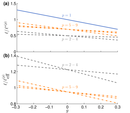
Figure 1: (Color online only) Evolution of (a) the transport coefficient, $1/\ell^{*(p)}$, and (b) the attenuation coefficient, $1/\ell_{\text{eff}}^{(p)}$, of polarization eigenmodes with short-range structural correlations. The coefficients are given in units of $1/\ell$ and shown on a restricted range of $g$ since the model is expected to remain valid to first order near $g=0$. The scalar mode ($p=1$, cyan solid curve) has a transport coefficient scaling as $(1-g)$ and an attenuation coefficient equal to zero (not shown). The polarization modes $p=2$–$4$ (gray dashed curves) and $p=5$–$9$ (orange dot-dashed curves) exhibit different slopes, indicating that both their transport properties are affected differently by short-range structural correlations.

IV Discussion

Previous studies based on the multiple scattering theory for the propagation of polarized light relied on the direct resolution of the Bethe-Salpeter equation, Eq. (9), using an expansion of the average Green’s tensors and its correlation function to order $K^{2}$ (diffusion approximation). This strategy is however possible only for uncorrelated disorder, for which $f(\boldsymbol{\mathbf{q}}-\boldsymbol{\mathbf{q}}^{\prime})=1$. Here, we proposed an alternative strategy based on the derivation of a transport equation taking the form of an RTE, which allowed us to reach the same final goal (eigenmode decomposition) including short-range structural correlations. This strategy, however, involves an additionnal approximation that has some implications. To clarify this point, let us consider our predictions in the limit of an uncorrelated disorder. Setting $g=0$ in the predictions of Table 1 yields the values reported in Table 2. An alternative straightforward derivation from Eqs. (32) and (33), which yields the same results, is proposed in Appendix C. Compared to previous results (see, e.g., Ref. Vynck et al., 2014), we observe that the eigenvectors, or polarization eigenchannels, remain unchanged, but the eigenvalues are now 1, 3 and 5-fold degenerate, yielding the same attenuation coefficients $\mu_{a}^{(p)}$ but different diffusion constants $\mathcal{D}^{(p)}$. This apparent discrepancy can be explained by the on-shell approximation, which “smoothes out” the polarization dependence in the correlation function of Green’s tensor. Nevertheless, it is important to note that the average diffusion constants for the various degenerate modes are strictly identical:

$$\frac{1}{3}\left(\frac{6}{5}c\ell+2\frac{2}{5}c\ell\right)=2\frac{c\ell}{3},$$ (41)

and

$$\frac{1}{5}\left(2\frac{230}{343}c\ell+2\frac{130}{343}c\ell+\frac{290}{1029}c\ell\right)=\frac{10}{7}\frac{c\ell}{3}$$ (42)

This brings us to the conclusion that the model is consistent with the approximations that have been made.

Table 2: Summary of the diffusion constants $\mathcal{D}^{(p)}$, attenuation coefficients $\mu_{a}^{(p)}$ and effective attenuation lengths $\ell_{\text{eff}}^{(p)}$ characterizing the diffusion properties of the energy density through the individual polarization eigenchannels for an uncorrelated disorder ($g=0$).

$p$	1	2-4	5-9
$\mathcal{D}^{(p)}$	$\frac{c\ell}{3}$	$2\frac{c\ell}{3}$	$\frac{10}{7}\frac{c\ell}{3}$
$\mu_{a}^{(p)}$	$0$	$\frac{1}{\ell}$	$\frac{3}{7\ell}$
$\ell_{\text{eff}}^{(p)}$	$\infty$	$\sqrt{\frac{2}{3}}\ell$	$\frac{\sqrt{10}}{3}\ell$

A second point deserving a comment is the fact that the attenuation length $1/\mu_{a}^{(p)}$ of the polarization eigenmodes does not depend on $g$ to first order, the effect of short-range structural correlations on the spatial decay of polarization away from the source being implemented via the definition of mode-specific transport mean free paths. This picture contrasts with previous studies based on the phenomenological transfer matrix approach Xu and Alfano (2005b); Rojas-Ochoa et al. (2004b), which relate the depolarization length $\ell_{p}$ for linearly polarized light to the scalar transport mean free path via a linear relation with $g$. In this sense, our model provides a different perspective on this basic problem of light transport in disordered media. Intuitively, this picture also appears more physically sound, since it is known that the relation between depolarization and transport mean free path varies with the incident polarization (linear, circular) or in presence of magneto-optical effects MacKintosh and John (1988); van Tiggelen et al. (1996).

Related to this point, it is also important to discuss the validity of the diffusion limit to retrieve depolarization coefficients. Reaching the regime of diffusive transport typically requires light to experience several multiple scattering events. However, as pointed out previously (see, e.g., Ref. Gorodnichev et al., 2014), this limit can hardly be achieved for the polarization modes, for which the depolarization occurs on the scale of a mean free path. It is then legitimate to question the accuracy of the expressions reported in Table 1. Nevertheless, we do not expect this question to impact our claim that different polarization modes are individually and differently affected by short-range structural correlations. Actually, the established RTE for the polarization-resolved specific intensity, Eq. (22), like the standard vector radiative transfer equation, does not assume diffusive transport. On this aspect, our study constitutes a very good starting point to investigate the validity of the diffusion approximation, which may be done either numerically by solving the RTE by Monte-Carlo methods, or analytically by adding higher-order Legendre polynomials $P_{n}$ in the following steps.

Finally, let us remark that the results of our model, in which disorder is described by a continuous and randomly fluctuating function of position [Eq. (1)], should apply not only to heterogeneous materials with complex textitconnected morphologies (e.g., porous media) but also to random ensembles of finite-size scatterers. Indeed, the Fourier transform of the structural correlation $f(\boldsymbol{\mathbf{r}}-\boldsymbol{\mathbf{r}}^{\prime})$ directly leads to the definition of the phase function $p(\hat{\boldsymbol{\mathbf{q}}}\cdot\hat{\boldsymbol{\mathbf{q}}}^{\prime})$ [Eq. (21)], which is the same function to which one arrives when investigating light scattering by finite-size scatterers (it is, in this case, defined from the differential scattering cross-section). For the sake of broadness of applications and convenience, the final results here have been given for the HG phase function [Eq. (36)] but other phase functions (e.g., Mie for spherical scatterers) may be used to describe specific disordered media. Note that for ensembles of finite-size scatterers, the short-range correlation approximation restricts the validity range of the model to small scatterers.

V Conclusion

To conclude, we have proposed a model based on multiple scattering theory to describe the propagation of polarized light in disordered media exhibiting short-range structural correlations. Our results assume weak disorder ($k_{0}\ell\gg 1$), short-range structural correlations (first order in $g$), and are obtained in the ladder approximation. Starting from the exact Dyson and Bethe-Salpeter equations for the average field and the field correlation, we have derived a RTE for the polarization-resolved specific intensity [Eq. (22)] and applied the $P_{1}$ approximation to investigate the propagation of polarized light in the diffusion limit. Interestingly, we have found that the polarization modes, described so far for uncorrelated disorder only, are independently and differently affected by short-range structural correlations. In practice, each mode is described by its own transport mean free path, which does not trivially depend on $g$ (see Table 1).

In essence, our study partly unveils the intricate relation between the complex morphology of disordered media and the polarization properties of the scattered intensity. The road towards a possible description of polarization-related mesoscopic phenomena in correlated disorder is long, yet we hope that the present work, which highlights several theoretical challenges when dealing with polarized light and structural correlations, will motivate future investigations. The model may be generalized, for instance, by including the most-crossed diagrams in the derivation to enable the study of phenomena such as weak localization, or frequency dependence to investigate —via a generalized RTE— the temporal response to incident light pulses. Another line of research could be to study the impact of short-range structural correlations on spatial coherence properties, which appears extremely relevant to the optical characterization of complex nanostructured media Dogariu and Carminati (2015).

Appendix A Average Green’s tensor

The average Green’s tensor $\left\langle\boldsymbol{\mathbf{G}}\right\rangle$ describes the propagation of the average field in the disordered medium and is related to the free-space Green’s tensor $\boldsymbol{\mathbf{G}}_{0}$ via the Dyson equation Akkermans and Montambaux (2011); Sheng (2010)

$$\left\langle\boldsymbol{\mathbf{G}}(\boldsymbol{\mathbf{q}})\right\rangle=\boldsymbol{\mathbf{G}}_{0}(\boldsymbol{\mathbf{q}})+\boldsymbol{\mathbf{G}}_{0}(\boldsymbol{\mathbf{q}})\boldsymbol{\mathbf{\Sigma}}(\boldsymbol{\mathbf{q}})\left\langle\boldsymbol{\mathbf{G}}(\boldsymbol{\mathbf{q}})\right\rangle,$$ (43)

where $\boldsymbol{\mathbf{\Sigma}}$ is the self-energy, which contains the sums over all multiply scattered events that cannot be factorized because of the average process. The free-space Green’s tensor is given by

$$\boldsymbol{\mathbf{G}}_{0}(\boldsymbol{\mathbf{q}}) =\left[(k_{0}^{2}-q^{2})\boldsymbol{\mathbf{I}}+\boldsymbol{\mathbf{q}}\otimes\boldsymbol{\mathbf{q}}\right]^{-1}$$ (44)

$$=\left[k_{0}^{2}\boldsymbol{\mathbf{I}}-q^{2}\boldsymbol{\mathbf{P}}(\hat{\boldsymbol{\mathbf{q}}})\right]^{-1},$$

with $\boldsymbol{\mathbf{P}}(\hat{\boldsymbol{\mathbf{q}}})=\boldsymbol{\mathbf{I}}-\hat{\boldsymbol{\mathbf{q}}}\otimes\hat{\boldsymbol{\mathbf{q}}}$. The average Green’s tensor then reads

$$\left\langle\boldsymbol{\mathbf{G}}(\boldsymbol{\mathbf{q}})\right\rangle =\left[\boldsymbol{\mathbf{I}}-\boldsymbol{\mathbf{G}}_{0}(\boldsymbol{\mathbf{q}})\boldsymbol{\mathbf{\Sigma}}(\boldsymbol{\mathbf{q}})\right]^{-1}\boldsymbol{\mathbf{G}}_{0}(\boldsymbol{\mathbf{q}})$$ (45)

$$=\left[k_{0}^{2}\boldsymbol{\mathbf{I}}-q^{2}\boldsymbol{\mathbf{P}}(\hat{\boldsymbol{\mathbf{q}}})-\boldsymbol{\mathbf{\Sigma}}(\boldsymbol{\mathbf{q}})\right]^{-1}.$$

By identification between Eq. (44) and Eq. (45), one can define an effective wavevector $\boldsymbol{\mathbf{q}}_{\text{eff}}=k_{0}^{2}\boldsymbol{\mathbf{\epsilon}}_{\text{eff}}(\boldsymbol{\mathbf{q}})$, where $\boldsymbol{\mathbf{\epsilon}}_{\text{eff}}(\boldsymbol{\mathbf{q}})=\boldsymbol{\mathbf{I}}-\boldsymbol{\mathbf{\Sigma}}(\boldsymbol{\mathbf{q}})/k_{0}^{2}$ is the effective medium permittivity tensor, yielding

$$\left\langle\boldsymbol{\mathbf{G}}(\boldsymbol{\mathbf{q}})\right\rangle=\left[\boldsymbol{\mathbf{q}}_{\text{eff}}^{2}-q^{2}\boldsymbol{\mathbf{P}}(\hat{\boldsymbol{\mathbf{q}}})\right]^{-1}.$$ (46)

In a dilute (3D) medium, interferences between successive scattering events can be neglected, and the self-energy can be calculated keeping only the first term of the multiple-scattering expansion

$$\boldsymbol{\mathbf{\Sigma}}(\boldsymbol{\mathbf{r}},\boldsymbol{\mathbf{r}}^{\prime}) \simeq k_{0}^{4}\left\langle\delta\epsilon(\boldsymbol{\mathbf{r}})\boldsymbol{\mathbf{G}}_{0}(\boldsymbol{\mathbf{r}}-\boldsymbol{\mathbf{r}}^{\prime})\delta\epsilon(\boldsymbol{\mathbf{r}}^{\prime})\right\rangle,$$

$$=uk_{0}^{4}f(\boldsymbol{\mathbf{r}}-\boldsymbol{\mathbf{r}}^{\prime})\boldsymbol{\mathbf{G}}_{0}(\boldsymbol{\mathbf{r}}-\boldsymbol{\mathbf{r}}^{\prime}),$$ (47)

or in reciprocal space

$$\boldsymbol{\mathbf{\Sigma}}(\boldsymbol{\mathbf{q}})=uk_{0}^{4}\int f(\boldsymbol{\mathbf{q}}-\boldsymbol{\mathbf{q}}^{\prime})\boldsymbol{\mathbf{G}}_{0}(\boldsymbol{\mathbf{q}}^{\prime})\frac{d\boldsymbol{\mathbf{q}}^{\prime}}{8\pi^{3}}.$$ (48)

For a delta-correlated disorder, $f(\boldsymbol{\mathbf{q}}-\boldsymbol{\mathbf{q}}^{\prime})=1$, we have

$$\operatorname{Im}\boldsymbol{\mathbf{\Sigma}}(\boldsymbol{\mathbf{q}})=-uk_{0}^{4}\frac{q}{6\pi}\boldsymbol{\mathbf{I}}.$$ (49)

The real part of $\boldsymbol{\mathbf{\Sigma}}$, which is typically very small for dilute media, is scalar as well. The effective medium permittivity then becomes a scalar quantity:

$$\boldsymbol{\mathbf{\epsilon}}_{\text{eff}}\simeq 1-\frac{\operatorname{Re}\Sigma(q)}{k_{0}^{2}}-i\frac{uk_{0}^{2}q}{6\pi}.$$ (50)

This allows rewriting Eq (45), after some algebra, as Tai (1993)

$$\left\langle\boldsymbol{\mathbf{G}}(\boldsymbol{\mathbf{q}})\right\rangle=\frac{1}{k_{0}^{2}\epsilon_{\text{eff}}-q^{2}}\left[\boldsymbol{\mathbf{I}}-\frac{\boldsymbol{\mathbf{q}}\otimes\boldsymbol{\mathbf{q}}}{k_{0}^{2}\epsilon_{\text{eff}}}\right],$$ (51)

which is equivalent to Eq. (11).

The coherent (ballistic) intensity in a disordered medium $I_{\text{coh}}=|\left\langle\boldsymbol{\mathbf{E}}\right\rangle|^{2}$ decays exponentially following the Beer-Lambert law

$$I_{\text{coh}}(z) =I_{\text{coh}}(0)\exp\left[-2k_{0}\operatorname{Im}(n_{\text{eff}})z\right],$$

$$=I_{\text{coh}}(0)\exp\left[-z/\ell\right],$$ (52)

with $\ell=(2k_{0}\operatorname{Im}[n_{\text{eff}}])^{-1}$ the extinction length, $n_{\text{eff}}=\sqrt{\epsilon_{\text{eff}}}$ the effective refractive index and $z$ the propagation direction. Since $\operatorname{Im}\epsilon_{\text{eff}}\ll\operatorname{Re}\epsilon_{\text{eff}}$ (i.e. $-\operatorname{Im}\Sigma\ll k_{0}^{2}$), we have $\operatorname{Im}(n_{\text{eff}})\simeq-\operatorname{Im}\Sigma/(2k_{0}q)$, thereby leading to

$$\operatorname{Im}\Sigma(\boldsymbol{\mathbf{q}})=-\frac{q}{\ell},\qquad u=\frac{6\pi}{k_{0}^{4}\ell}.$$ (53)

For an arbitrary (non-delta) correlated disorder $f(\boldsymbol{\mathbf{q}}-\boldsymbol{\mathbf{q}}^{\prime})\neq 1$, Eq. (A) indicates that $\boldsymbol{\mathbf{\Sigma}}$ should not be a scalar. Thus, the average Green’s tensor in Eq. (45) cannot possibly take the form of Eq. (51); and Eq. (53), which introduces the mean free path $\ell$ in the RTE [Eq. (22)], should be corrected. Our results are therefore expected to be strictly valid only for short-range structural correlations (close to a delta-correlated potential), i.e. for scattering anisotropy factors $g$ close to 0.

Appendix B Short-range correlation approximation

As explained above, due to the fact that the self-energy $\boldsymbol{\mathbf{\Sigma}}$ is assumed to be a scalar quantity in our model, our theoretical predictions are expected to be valid only for short-range structural correlations, i.e. for $g$ close to zero. The validity range of this approximation can be apprehended by comparing the raw prediction obtained from the eigenmode decomposition, Eq. (35), without performing the development to order $g$, with predictions from scalar theory. The eigenmode decomposition for the scalar mode, in the diffusion approximation (i.e., to order $K^{2}$), yields a transport mean free path

$$\ell^{*(1)}=\frac{10+g(5g-2)}{10+g(5g-12)}\ell,$$ (54)

to be compared with the expected relation, $\ell^{*}=\ell(1-g)^{-1}$. The two relations are shown in Fig. 2, where it is found that our prediction remains fairly good for $-0.3\lesssim g\lesssim 0.3$, hence the range chosen in Fig. 1. Developing the transport coefficient $1/\ell^{*(1)}$ of Eq. (54) to order $g$ yields the proper $(1-g)$ scaling, as reported in Table 1.

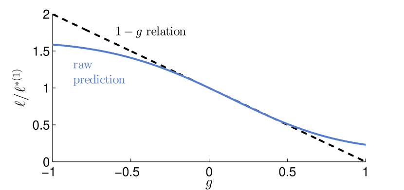
Figure 2: (Color online only) Evolution of the transport coefficient of the scalar mode, $1/\ell^{*(1)}$, in units of $1/\ell$, with the scattering anisotropy factor $g$. We compare the raw prediction obtained from the eigenmode decomposition, Eq. (35), before the development to order $g$ (solid cyan curve), with the expected $1-g$ scaling relation (black dashed curve). Our theoretical predictions are expected to be valid for short-range structural correlations, i.e. for $g$ close to zero.

Appendix C Eigenmode decomposition for uncorrelated disorder

For uncorrelated disorder, the scattering anisotropy factor $g$ equals zero, such that, from Eq. (33), we immediately obtain

$$i\boldsymbol{\mathbf{K}}\cdot\boldsymbol{\mathbf{j}}_{ijkl}(\boldsymbol{\mathbf{K}})=\frac{4\pi}{3}K^{2}\ell L^{(0)}_{ijkl}(\boldsymbol{\mathbf{K}}).$$ (55)

Inserting it into Eq. (32), we get

$$\frac{4\pi}{3} K^{2}\ell L^{(0)}_{ijkl}(\boldsymbol{\mathbf{K}})+\frac{4\pi}{\ell}L^{(0)}_{ijkl}(\boldsymbol{\mathbf{K}})$$

$$=\frac{2}{3}S_{ijkl}+\frac{4\pi}{\ell}S_{ijmn}L^{(0)}_{mnkl}(\boldsymbol{\mathbf{K}}).$$ (56)

Performing an eigenmode decomposition of $S_{ijkl}$ as

$$S_{ijkl}=\sum_{p=1}^{9}S^{(p)}\left|ij\right\rangle^{(p)}\left\langle kl\right|^{(p)},$$ (57)

and similarly for $L^{(0)}_{ijkl}=c/(6\pi)U_{ijkl}$, we directly find that the diffusion of the energy density in each polarization eigenchannel, $U^{(p)}$, follows the solution of the diffusion equation, Eq. (39), with

$$\mathcal{D}^{(p)}=\frac{c\ell}{3}\frac{1}{S^{(p)}},\qquad\mu_{a}^{(p)}=\frac{1}{\ell}\frac{1-S^{(p)}}{S^{(p)}}.$$ (58)

The eigenvalues of $S_{ijkl}$ are $1$, $1/2$ and $7/10$ with degeneracies $1$, $3$ and $5$, respectively, thereby leading to the values reported in Table 2.

References

• Akkermans and Montambaux (2011) E. Akkermans and G. Montambaux, Mesoscopic Physics of Electrons and Photons (Cambridge University Press, 2011).
• Sheng (2010) P. Sheng, Introduction to Wave Scattering, Localization and Mesoscopic Phenomena (Springer, 2010).
• Goodman (2015) J. W. Goodman, Statistical Optics (Wiley, 2015).
• Brosseau (1998) C. Brosseau, Fundamentals of Polarized Light: A Statistical Optics Approach (Wiley-Blackwell, 1998).
• Tuchin et al. (2006) V. V. Tuchin, L. Wang, and D. A. Zimnyakov, Optical Polarization in Biomedical Applications (Springer, 2006).
• Maradudin (2007) A. A. Maradudin, ed., Light Scattering and Nanoscale Surface Roughness (Springer, 2007).
• Andrews and Phillips (2005) L. C. Andrews and R. L. Phillips, Laser Beam Propagation through Random Media (SPIE, 2005).
• Shirai et al. (2003) T. Shirai, A. Dogariu, and E. Wolf, J. Opt. Soc. Am. A 20, 1094 (2003).
• Apostol and Dogariu (2003) A. Apostol and A. Dogariu, Phys. Rev. Lett. 91, 093901 (2003).
• Carminati (2010) R. Carminati, Phys. Rev. A 81, 1 (2010).
• Parigi et al. (2016) V. Parigi, E. Perros, G. Binard, C. Bourdillon, A. Maître, R. Carminati, V. Krachmalnicoff, and Y. De Wilde, Opt. Express 24, 7019 (2016).
• Cazé et al. (2010) A. Cazé, R. Pierrat, and R. Carminati, Phys. Rev. A 82, 043823 (2010).
• Sapienza et al. (2011) R. Sapienza, P. Bondareff, R. Pierrat, B. Habert, R. Carminati, and N. F. Van Hulst, Phys. Rev. Lett. 106, 1 (2011).
• Schmidt et al. (2015) M. K. Schmidt, J. Aizpurua, X. Zambrana-Puyalto, X. Vidal, G. Molina-Terriza, and J. J. Sáenz, Phys. Rev. Lett. 114, 113902 (2015).
• Torquato (2005) S. Torquato, Random Heterogeneous Materials: Microstructure and Macroscopic Properties (Springer, 2005).
• Rojas-Ochoa et al. (2004a) L. F. Rojas-Ochoa, J. M. Mendez-Alcaraz, J. J. Sáenz, P. Schurtenberger, and F. Scheffold, Phys. Rev. Lett. 93, 73903 (2004a).
• García et al. (2007) P. García, R. Sapienza, Á. Blanco, and C. López, Adv. Mater. 19, 2597 (2007).
• MacKintosh et al. (1989) F. C. MacKintosh, J. X. Zhu, D. J. Pine, and D. A. Weitz, Phys. Rev. B 40, 9342 (1989).
• Xu and Alfano (2005a) M. Xu and R. R. Alfano, Phys. Rev. E. Stat. Nonlin. Soft Matter Phys. 72, 065601 (2005a).
• Gorodnichev et al. (2007) E. E. Gorodnichev, A. I. Kuzovlev, and D. B. Rogozkin, J. Exp. Theor. Phys. 104, 319 (2007).
• Skipetrov and Sokolov (2014) S. E. Skipetrov and I. M. Sokolov, Phys. Rev. Lett. 112, 23905 (2014).
• Bellando et al. (2014) L. Bellando, A. Gero, E. Akkermans, and R. Kaiser, Phys. Rev. A 90, 063822 (2014).
• Edagawa et al. (2008) K. Edagawa, S. Kanoko, and M. Notomi, Phys. Rev. Lett. 100, 1 (2008).
• Liew et al. (2011) S. F. Liew, J.-K. Yang, H. Noh, C. F. Schreck, E. R. Dufresne, C. S. O’Hern, and H. Cao, Phys. Rev. A 84, 63818 (2011).
• Imagawa et al. (2010) S. Imagawa, K. Edagawa, K. Morita, T. Niino, Y. Kagawa, and M. Notomi, Phys. Rev. B 82, 115116 (2010).
• Chandrasekhar (1960) S. Chandrasekhar, Radiative Transfer (Dover Publications, 1960).
• Papanicolaou and Burridge (1975) G. C. Papanicolaou and R. Burridge, J. Math. Phys. 16, 2074 (1975).
• Mishchenko and Travis (2006) M. I. Mishchenko and L. D. Travis, Multiple Scattering of Light by Particles: Radiative Transfer and Coherent Backscattering (Cambridge University Press, 2006).
• Amic et al. (1997) E. Amic, J. M. Luck, and T. M. Nieuwenhuizen, J. Phys. I 7, 445 (1997).
• Gorodnichev et al. (2014) E. E. Gorodnichev, A. I. Kuzovlev, and D. B. Rogozkin, Phys. Rev. E 90, 043205 (2014).
• Akkermans et al. (1988) E. Akkermans, P. Wolf, R. Maynard, and G. Maret, J. Phys. 49, 77 (1988).
• Xu and Alfano (2005b) M. Xu and R. R. Alfano, Phys. Rev. Lett. 95, 213901 (2005b).
• Rojas-Ochoa et al. (2004b) L. F. Rojas-Ochoa, D. Lacoste, R. Lenke, P. Schurtenberger, and F. Scheffold, J. Opt. Soc. Am. A. Opt. Image Sci. Vis. 21, 1799 (2004b).
• Stephen and Cwilich (1986) M. J. Stephen and G. Cwilich, Phys. Rev. B 34, 7564 (1986).
• MacKintosh and John (1988) F. C. MacKintosh and S. John, Phys. Rev. B 37, 1884 (1988).
• Ozrin (1992) V. D. Ozrin, Waves in Random Media 2, 141 (1992).
• van Tiggelen et al. (1996) B. van Tiggelen, R. Maynard, and T. Nieuwenhuizen, Phys. Rev. E 53, 2881 (1996).
• van Tiggelen et al. (1999) B. A. van Tiggelen, A. Lagendijk, and A. Tip, J. Phys. Condens. Matter 2, 7653 (1999).
• Müller and Miniatura (2002) C. A. Müller and C. Miniatura, J. Phys. A Math. Gen. 35, 10163 (2002).
• Vynck et al. (2014) K. Vynck, R. Pierrat, and R. Carminati, Phys. Rev. A 89, 013842 (2014).
• Setälä et al. (2002) T. Setälä, A. Shevchenko, M. Kaivola, and A. T. Friberg, Phys. Rev. E 66, 1 (2002).
• Dennis (2007) M. R. Dennis, J. Opt. Soc. Am. A 24, 2065 (2007).
• Réfrégier et al. (2014) P. Réfrégier, V. Wasik, K. Vynck, and R. Carminati, Opt. Lett. 39, 2362 (2014).
• Gil (2014) J. J. Gil, Phys. Rev. A 90, 043858 (2014).
• Dogariu and Carminati (2015) A. Dogariu and R. Carminati, Phys. Rep. 559, 1 (2015).
• Tai (1993) C. Tai, Dyadic Green Functions in Electromagnetic Theory (IEEE Press, New-York, 1993).
• Arnoldus (2003) H. F. Arnoldus, J. Mod. Opt. 50, 755 (2003).
• (48) Wolfram Mathematica.
• Henyey and Greenstein (1941) L. C. Henyey and J. L. Greenstein, Astrophys. J. 93, 70 (1941).