SALZA: Soft algorithmic complexity estimates for clustering and causality inference

Abstract

A complete set of practical estimators for the conditional, simple and joint algorihmic complexities is presented, from which a semi-metric is derived. Also, new directed information estimators are proposed that are applied to causality inference on Directed Acyclic Graphs. The performances of these estimators are investigated and shown to compare well with respect to the state-of-the-art Normalized Compression Distance (NCD [1]).

I Introduction

The use of compression algorithms to extract information from sequences or strings has found applications in various fields [2] (and references therein), from biomedical and EEG time series analysis [3][4] to languages classification [5] or species clustering [5]. Since the early papers of Lempel and Ziv [6], the use of Kolmogorov complexity (the length of a shortest program able to output the input string on a universal Turing computer [2]) in place of entropy for non-probabilistic study of bytes strings, signals or digitized objects has led to the developement of the Algorithmic Information Theory (AIT) [2]. Amongst the very interesting ideas and concepts in AIT, the possiblity of defining distances between objects to measure their similitudes, i.e. how much information they share, is one of the most used in practice.

The approach proposed here was initially motivated by getting rid of most limitations induced be the use of a practical compressor in computing an information distance [7]. Reimplementing a coder from scratch allowed to give access to a much richer information than the raw length of a compressed file (the only information available when using “off-the-shelf” compressors). Doing so also allows to propose new estimates for simple, conditional and joint algorihmic complexities. Such estimates can lead to the definition of a soft information semi-distance, as well as directed information estimates.

The maximum information distance between two strings $x$ and $y$ is defined as [8]:

$$E_{1}(x,y)=\mbox{max}\{K(x|y),K(y|x)\},$$ (1)

where $K(x|y)$ denotes the conditional Kolmogorov complexity of $x$ given $y$: the size of a shortest program able to output $x$ knowing $y$. The Kolmogorov complexity $K$ is known not to be computable on a universal Turing computer. Note that we will later extend the meaning of the conditional sign in Sec. II-A.

In order to compare objects of different sizes, the Normalized Information Distance (NID) has been proposed [1]:

$$\mbox{NID}(x,y)=\frac{\mbox{max}\{K(x|y),K(y|x)\}}{\mbox{max}\{K(x),K(y)\}},$$ (2)

where $K(x)$ denotes the Kolmogorov complexity of $x$: the size of a shortest program able to output $x$ on a universal computer. Since $K$ is not computable, one usually has to resort to two main approximations, leading to the Normalized Compression Distance (NCD) [1], which is a practical embodiment of the NID.

Let $xy$ be the concatenation of $x$ and $y$. The first approximation concerns $K(x|y)$, which then reads [1]:

$$K(x|y)\approx K(xy)-K(y).$$ (3)

The second approximation consists in using the output of a real-world compressor to estimate $K$. Let $C(x)$ be the compressed version of $x$ by a given compressor, the NCD then reads [1]:

$$\mbox{NCD}(x,y)=\frac{C(xy)-\mbox{min}\{C(x),C(y)\}}{\mbox{max}\{C(x),C(y)\}}.$$ (4)

It is remarkable that any compressor can be used to estimate the NCD (actually, the results are consistent even across families of compressors). However, it is our goal to show that a particular family of compressors, namely those based on the Lempel-Ziv algorithm [9], are more amenable than others (namely, block-based) to mitigate the limitations induced by Eq. (3).

Using real-world compressors brings mainly two major limitations:

• The size of the block for block-based compressors [7];

• For LZ77-based compressors:

  1. The size of the sliding window. For example, the DEFLATE [10] compressor has a sliding window of 32KiB. Obviously, when the length of $y$ is greater than the size of the sliding window, then $C(xy)$ may not always use strings from $x$ to encode $y$. Note that increasing the size of the sliding window (e.g., [11]) does not guarantee that only strings from $x$ will be used to encode $y$;

  2. The size of the substrings that can be found in $y$ to encode $x$ is limited (258 bytes for DEFLATE).

The rest of this paper is organized as follows: After introducing four possible types of conditional information in Sec II-A, we propose in Sec. II-B a normalized conditional algorithmic complexity estimate. We also give the expressions for simple and joint complexity estimates (Sec. II-D) and come up with a normalized information semi-distance (Sec. III-A). This is in contrast with previous approaches were the normalization was performed afterwards. Then in Sec. IV-A we compare our semi-distance with the NCD. Finally, we define our algorithmic complexity estimates for directed information III-B and apply them to causality inference on directed acyclic graphs in Sec. IV-B.

II SALZA

The rationale for SALZA is to come up with a practical implementation of algorithmic complexity estimates that could work continuously over any sequence of symbols. This discards block-based compression method like e.g., bzip2 which uses the Burrows-Wheeler block transform.

As a practical implementation of [9] targeted towards data compression, DEFLATE has to finely tune the intricacy between the string searching stage and the entropy coding stage. For example, DEFLATE will generally use a socalled lazy match string searching strategy, meaning it will not necessarily find the longest strings, but stop the search at appropriate lengths. This has the combined effect of speeding up the overall compression time, and also it produces a lengths distribution that is more peaked (and hence more amenable to compression). However, it artificially creates references to shorter strings that hence are not the most meaningful to explain the input data.

Therefore, we explicitly depart from the pure data compression approach to compute our algorithmic complexity estimates, but we keep Ziv-Merhav [12] and LZ77 [9] as the core building blocks of our strategy. In the following, all substrings are the longest substrings. For the same reason, we do not use the entropy coding stage.

II-A Conditional information

SALZA builds on an implementation of DEFLATE [10] that has been further extended with an unbounded buffer in order to implement the computation of a conditional Kolomogorov complexity estimate. SALZA will factorize a string $x$ using conditional information that may come from different sets of strings. The string of possible references is denoted $\mathcal{R}$ and its alphabet is $\mathcal{A}_{\mathcal{R}}$. We use the following to denote the four possible reference strings, each time with respect to the current encoding position of the lookahead buffer:

1. ${y}_{\mbox{\small}}|^{\mbox{\tiny}}{x}$: $\mathcal{R}$ is only the past of $x$:

   This models the usual LZ77 operating mode when $x=y$ (needed in Sec. II-D), and $\mathcal{A}_{\mathcal{R}}=\mathcal{A}_{x}$;

2. ${y}_{\mbox{\small}}|^{\mbox{\tiny+}}{x}$: $\mathcal{R}$ is all of $x$:

   This models the usual Ziv-Merhav operating mode (needed in Sec. II-B), and $\mathcal{A}_{\mathcal{R}}=\mathcal{A}_{x}$;

3. ${y}_{\mbox{\small-}}|^{\mbox{\tiny}}{x}$: $\mathcal{R}$ is the past of both $x$ and $y$:

   This will be needed later on in Sec. III-B, and $\mathcal{A}_{\mathcal{R}}=\mathcal{A}_{x}\cup\mathcal{A}_{y}$;

4. ${y}_{\mbox{\small-}}|^{\mbox{\tiny+}}{x}$: $\mathcal{R}$ is the past of $y$ and all of $x$:

   This will be needed later on in Sec. II-D, and $\mathcal{A}_{\mathcal{R}}=\mathcal{A}_{x}\cup\mathcal{A}_{y}$;

These types of conditional informations are depicted in Fig. (1). When the conditional information is left unspecified, we will use ${x}\wr{y}$ to stand for either type of conditional information.

Figure 1: Strings $\mathcal{R}$ for the conditional information (from which references are allowed), by darkening shades of gray: ${y}_{\mbox{\small-}}|^{\mbox{\tiny+}}{x}$, ${y}_{\mbox{\small-}}|^{\mbox{\tiny}}{x}$, ${y}_{\mbox{\small}}|^{\mbox{\tiny+}}{x}$ and ${y}_{\mbox{\small}}|^{\mbox{\tiny}}{x}$. The thick vertical bar represents the position of the current lookahead buffer when encoding $y$.

Using any conditional information of the above, SALZA will always produce symbols of the form $\left(l,v\right)$, which can be either:

• references: $l>1$ is the length of a substring in the dictionary, and, although it is not used in this paper, $v$ is the offset in the dictionary at which bytes should start to be copied;

• literals: $l=1$ and $v$ is the literal in $x$ that should be copied to the output buffer.

It is important to notice that for any output symbol of SALZA, one has that:

$$\forall l,l\geq 1.$$ (5)

Eventually, SALZA will factorize a string $x$ in $n$ symbols by finding always the longest strings (and $n$ will be our estimate of the relative complexity [12] when SALZA is run in Ziv-Merhav mode):

$$x\rightsquigarrow\left(l_{1},v_{1}\right)\ldots\left(l_{n},v_{n}\right).$$

A specific feature of SALZA is that it gives access to a much richer information than when using an “out of the box” compressor. In particular, the lengths of the symbols produced during the factorization of a string allows to define a complexity measure that exhibits a stronger discriminative power than those available in the state-of-the-art litterature.

II-B The SALZA conditional complexity estimate

Let $\mathcal{L}_{{x}\wr{y}}=\left\{l\right\}$ be the reference lengths produced by the relative coding of $x$ given $y$ by SALZA using any conditional information. Also, $|.|$ denotes the length of a string or the cardinal of an alphabet. Note also that $x$ is defined over the alphabet $\mathcal{A}_{x}$ and $y$ is defined over $\mathcal{A}_{y}$. When strings $x$ and $y$ are defined over the same alphabet, it will be simply denoted $\mathcal{A}$.

When used in Ziv-Merhav mode ($\mathcal{L}_{{x}\wr{y}}=\mathcal{L}_{{x}_{\mbox{\small}}|^{\mbox{\tiny+}}{y}}$), SALZA will operate as follows:

• if $x$ and $y$ do not share the same alphabet, only literals will be produced;

• if $x=y$, only one symbol will be produced, namely $\left(|x|,1\right)$.

Definition II.1.

Set value.

Let $f:\mathbb{N}^{\star}\rightarrow\mathbb{R}$ be a mapping and let $\mathcal{T}$ be a finite set of non-zero natural numbers. The image of $\mathcal{T}$ by $f$ is defined as:

$$|\mathcal{T}|_{f}=\sum_{s\in\mathcal{T}}f(s).$$

The notation $|\mathcal{T}|=|\mathcal{T}|_{\mathbbm{1}_{\mathcal{T}}}$ will also be used to denote the cardinal of $\mathcal{T}$.

We now look for a normalized, conditional complexity estimate. Focusing on a conditional measure is the first step to proposing the semi-distance later on in Sec. III-A or constructing directed informations estimates in III-B. The very normalization, as in [1], is needed to compare objects of different sizes. In contrast with [1], our strategy is not to perform the normalization afterwards, but to use directly Eq. (1) with an already normalized estimate.

Definition II.2.

Admissible function.

A function $f:\mathbb{N}^{\star}\rightarrow\left[0,1\right]$ is said to be admissible iff it is monotonically increasing.

In the following definition, the admissible function allows us to finely modulate the information that is taken into account (see Sec. II-C).

Definition II.3.

SALZA conditional complexity estimate.

Given an admissible function $f$, and two non-empty strings $x\in\mathcal{A}_{x}$ and $y\in\mathcal{A}_{y}$, the SALZA conditional complexity estimate of $x$ given $y$, denoted $S_{f}({x}\wr{y})$, is defined as:

$$S_{f}({x}\wr{y})=\underbrace{\left(1-\frac{\sum_{\mathcal{L}_{{x}\wr{y}}}lf(l)-(|\mathcal{L}_{{x}\wr{y}}|_{f}-1)}{\left|x\right|}\right)}_{\mathcal{S}}\underbrace{\frac{|\mathcal{L}_{{x}\wr{y}}|-1}{|x|}}_{\mathcal{Z}}.$$ (6)

For simplicity, the dependency on $x$ $y$ and $f$ in the terms of the fatorization are omitted. Therefore, the form $S_{f}({x}\wr{y})={\mathcal{S}}{\mathcal{Z}}$ will be used in the sequel.

In Eq. (6), the two-terms factorization elements of $S_{f}({x}\wr{y})$ can be interpreted the following way:

1. ${\mathcal{S}}$ is based on the length ratio of $x$ that is explained by $y$ – we will show that it acts as a “spreading” factor that emphasizes differences between both strings so that the final value allows for a sharper numerical estimate (see Sec. II-C);

2. ${\mathcal{Z}}$ is the normalization of the SALZA approximation of the relative complexity [12]. This normalization is simply obtained by dividing by the maximum number of symbols that can be produced, namely $|x|$.

Lemma 1.

$0\leq S_{f}({x}\wr{y})<1.$

Proof.

The proof consists in demonstrating that both ${\mathcal{S}}$ and ${\mathcal{Z}}$ are normalized and follow the same trend with respect to similarity.

1. First, we show that the term ${\mathcal{S}}$ is normalized.

   Remark that:

   $$\sum_{\mathcal{L}_{{x}\wr{y}}}lf(l)-|\mathcal{L}_{{x}\wr{y}}|_{f}=\sum_{\mathcal{L}_{{x}\wr{y}}}f(l)(l-1).$$

   Because $f$ is upper-bounded by 1 and remembering that $l\geq 1$, see Eq. (5), then:

   $$\sum_{\mathcal{L}_{{x}\wr{y}}}f(l)(l-1)\leq\sum_{\mathcal{L}_{{x}\wr{y}}}(l-1),$$

   and:

   $$\sum_{\mathcal{L}_{{x}\wr{y}}}(l-1)\leq|x|-1.$$

   Note that the equality holds when $x$ is a substring of $\mathcal{R}$ (e.g., when computing $S_{f}({x}_{\mbox{\small}}|^{\mbox{\tiny+}}{x})$).

   Hence:

   $$\left(1-\frac{\sum_{\mathcal{L}_{{x}\wr{y}}}lf(l)-(|\mathcal{L}_{{x}\wr{y}}|_{f}-1)}{\left|x\right|}\right)\geq 0,$$

   with zero being reached when $x$ is a substring of $\mathcal{R}$.

   By Eq. (5) and positivity of $f$, one has:

   $$\sum_{\mathcal{L}_{{x}\wr{y}}}f(l)(l-1)\geq 0.$$

   Therefore:

   $$\left(1-\frac{\sum_{\mathcal{L}_{{x}\wr{y}}}lf(l)-(|\mathcal{L}_{{x}\wr{y}}|_{f}-1)}{\left|x\right|}\right)\leq 1,$$

   with equality being reached when $x$ and $\mathcal{R}$ are maximally dissimilar (e.g., $\mathcal{A}_{x}\cap\mathcal{A}_{y}=\emptyset$ when computing $S_{f}({x}_{\mbox{\small}}|^{\mbox{\tiny+}}{y})$).

2. Second, we show that ${\mathcal{Z}}$ is also normalized.

   The SALZA factorization will produce at least one symbol (exactly one when $x$ is a substring of $\mathcal{R}$), therefore:

   $$\frac{|\mathcal{L}_{{x}\wr{y}}|-1}{|x|}\geq 0.$$

   Note that ${\mathcal{Z}}$ only vanishes when $x=y$.

   In the worst case (when $x$ and $\mathcal{R}$ are maximally dissimilar, e.g. $\mathcal{A}_{x}\cap\mathcal{A}_{\mathcal{R}}=\emptyset$, same as above), $|\mathcal{L}_{{x}\wr{y}}|=|x|$. Therefore:

   $$\frac{|\mathcal{L}_{{x}\wr{y}}|-1}{|x|}=\frac{|x|-1}{|x|}<1.$$

From the above considerations, it is easy to see that, when $x$ and $y$ are maximally dissimilar, one has:

$$\lim_{|x|\rightarrow\infty}S_{f}({x}\wr{y})=1.$$

∎

Before making use of $S_{f}({x}\wr{y})$ to measure complexity, we investigate some of its features.

II-C Study of the SALZA conditional complexity estimate

We start by choosing an admissible function $f$. The use of $f$ in Eq. (6) allows to modulate the choice of the references taken into account, and how they contribute to the construction of the estimate of the complexity.

A possible choice for $f$ is a threshold function in order to filter out references that are not meaningful. Such references are first defined as explained below.

Definition II.4.

Meaningful references [6].

A SALZA reference $\left(l,v\right)$ is said to be meaningful with respect to $\mathcal{R}$ iff:

$$l>l^{0}_{\mathcal{R}}=\log_{|\mathcal{A}_{\mathcal{R}}|}\left|\mathcal{R}\right|.$$ (7)

Then, an admissible threshold function is defined as follows:

Definition II.5.

Threshold function.

The admissible threshold function for string $\mathcal{R}$, denoted $f_{\mathcal{R}}^{t}$, is defined as:

$$f_{\mathcal{R}}^{t}(l)=\left\{\begin{aligned} 1&&\mbox{if}&&l>l^{0}_{\mathcal{R}}\\ 0&&\mbox{otherwise}&\end{aligned}\right..$$

However, as expected, this choice produces discontinuities in the first term of $S_{f_{\mathcal{R}}^{t}}({x}\wr{y})$, i.e. ${\mathcal{S}}_{\mathcal{R}}^{t}$, see Fig. (2). The effect of using this threshold is especially harmful when $l_{\mathcal{R}}^{0}$ is close to $\lfloor l_{\mathcal{R}}^{0}\rfloor$: in that case, references which are just smaller than $l_{\mathcal{R}}^{0}$ are discarded, even though they may carry some information.

An easy way to circumvent this issue is to replace the threshold function with a continuous function in order to produce soft estimates. Among all possible choices, we arbitrarily favor $C^{\infty}$ functions and make use of a sigmoid.

Definition II.6.

Sigmoid function.

The admissible sigmoid function for string $\mathcal{R}$, denoted $f_{\mathcal{R}}^{s}$, is defined as:

$$f_{\mathcal{R}}^{s}(l)=\frac{1}{1+e^{-l+l_{\mathcal{R}}^{0}}}.$$

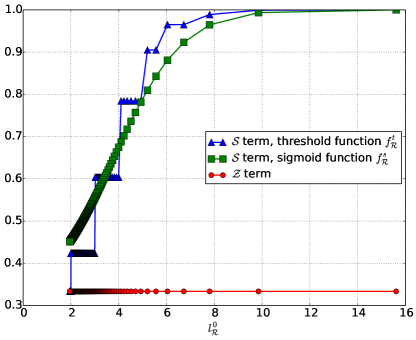
Figure 2: Profiles of $S_{f_{\mathcal{R}}^{t}}({x}\wr{y})$ (triangles) vs. $S_{f_{\mathcal{R}}^{s}}({x}\wr{y})$ (squares) as a function of $l_{\mathcal{R}}^{0}$. Using a continuous admissible function like a sigmoid allows to circumvent the effect of taking hard decisions when thresholding. This is especially important for small references and helps better discriminate dissimilar strings.

In the following, we study the evolution of the various scores with respect to $\mu$ the mean length of the symbols produced during the factorization, $|x|$ and $l_{\mathcal{R}}^{0}=\log_{|\mathcal{A}_{\mathcal{R}}|}\left|\mathcal{R}\right|$. This study is hardly tractable using closed-form expressions and we resort to numerical simulations (this is inspired by the probabilistic treatment found in [12]). From our experiments, we chose the Poisson distribution as the most suitable discrete distribution for the symbol lengths.

In order to study $S_{f}({x}\wr{y})$ with respect to $\mu$, we have fixed $l_{\mathcal{R}}^{0}$ and generated Poisson-distributed lengths such that $\sum_{\mathcal{L}_{{x}\wr{y}}}l=|x|$. The results are depicted in Fig. (3): when $\mu$ takes high values (i.e., $x$ and $\mathcal{R}$ contain many identical long strings) all three terms get the same. However, when $\mu$ is smaller (i.e., $x$ and $\mathcal{R}$ only contain short identical strings), then the spreading term $\mathcal{S}$ of SALZA in Eq. (6) will take much higher values than the term $\mathcal{Z}$ alone. Hence, the discriminative power of SALZA for dissimilar strings is expected to be much stronger.

In order to study $S_{f}({x}\wr{y})$ with respect to $|x|$, we have worked with both $\mu$ and $l_{\mathcal{R}}^{0}$ fixed. The results are depicted in Fig. (4): they confirm that the SALZA conditional complexity estimate is invariant with respect to $x$.

In Fig. (2), it is noticeable that the term $\mathcal{Z}$ is constant with respect to $l_{\mathcal{R}}^{0}$. This is actually an issue. Suppose $\mathcal{R}$ is a long string defined over a small alphabet, then it is very likely that $\mathcal{R}$ will contain almost all possible strings of small size. Thus, if $x$ is defined over the same small alphabet, there is a high chance that it will be explained using only small strings found in $\mathcal{R}$. Therefore, it seems important to take into account both the values of $|\mathcal{R}|$ and $|\mathcal{A}_{\mathcal{R}}|$ and this can be done using the minimal length of meaningful references $l_{\mathcal{R}}^{0}$.

Now, as opposed to the $\mathcal{Z}$ term, the “spreading” term of Eq. (6), i.e. ${\mathcal{Z}}$, will adapt to all settings. Using a sigmoid allows for a softer estimate than when using a threshold. This, in fact, contributes to the stronger discriminative power of SALZA when common substrings are close to $l_{\mathcal{R}}^{0}$, see Fig. (3).

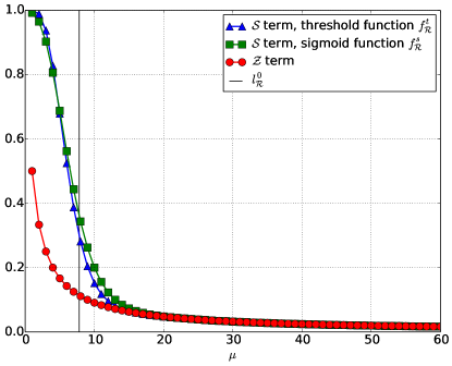
Figure 3: Discriminative power of SALZA as a function of the Poisson distribution mean $\mu$. The minimal value of the meaningful references $l_{\mathcal{R}}^{0}$ is represented as a vertical bar.

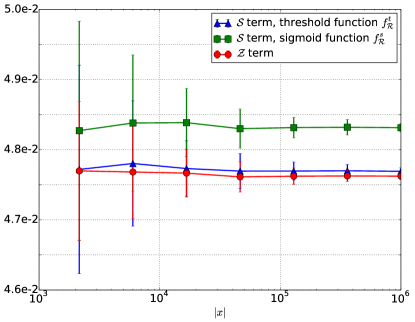
Figure 4: $S_{f_{\mathcal{R}}^{t}}({x}\wr{y})$ (triangles) and $S_{f_{\mathcal{R}}^{s}}({x}\wr{y})$ (squares) as a function of $|x|$. The discriminative power of SALZA is nearly constant for arbitrarily long strings – this is in contrast with the NCD (see Sec. IV-A) and it is due to the unbounded buffer in our implementation. Note that the plot starts when $|x|$ is half the size of the DEFLATE buffer. Each point has been generated by averaging 200 realizations.

Overall, the SALZA conditional complexity estimate will better discriminate dissimilar strings than the $\mathcal{Z}$ term alone, and it will do so equally well on arbitrarily long strings. As for the choice of the admissible function, we observe a little advantage in favor of the sigmoid. Therefore, in the rest of this paper, unless otherwise explicitly stated, the sigmoid is the default admissible function for all computations.

II-D SALZA complexity and joint complexity

Let $\mathcal{L}_{x}=\mathcal{L}_{{x}_{\mbox{\small}}|^{\mbox{\tiny}}{x}}$ be the set of lengths produced during a regular DEFLATE factorization (i.e., a close version of that in [9]). This allows us to propose an estimate for the joint complexity of strings $x$ and $y$.

Definition II.7.

SALZA complexity.

Given an admissible funtion $f$ and a non-empty string $x\in\mathcal{A}_{x}$, the SALZA complexity of $x$, denoted $S_{f}(x)$, is defined as:

$$S_{f}(x) =S_{f}({x}_{\mbox{\small}}|^{\mbox{\tiny}}{x})$$

$$=\left(1-\frac{\sum_{\mathcal{L}_{x}}lf(l)-(|\mathcal{L}_{x}|_{f}-1)}{\left|x\right|}\right)\frac{|\mathcal{L}_{x}|-1}{|x|}.$$

The joint Kolmogorov complexity can be understood as the minimal program length able to encode both $x$ and $y$, as well as a means to separate the two [2]. Hence, there is no need to restrict the references only to $x$, and we should allow references to the past of $y$ as well. In order to mimic the relationship $K(x,x)=K(x)$, we choose a length ratio as the way to separate both strings.

Definition II.8.

SALZA joint complexity.

Given an admissible function $f$, and two non-empty strings $x\in\mathcal{A}_{x}$ and $y\in\mathcal{A}_{y}$, the SALZA joint complexity of $x$ and $y$, denoted $S_{f}(x,y)$, is defined as:

$$S_{f}(x,y)=S_{f}({y}_{\mbox{\small-}}|^{\mbox{\tiny+}}{x})+S_{f}(x)+\log_{|\mathcal{A}_{x}|}\left(\frac{|x|}{|y|}\right).$$

Note that $S_{f}(x,x)=S_{f}(x)$ because $S_{f}({x}_{\mbox{\small-}}|^{\mbox{\tiny+}}{x})=0$.

In order to validate our approach, we measure the following absolute error:

$$\epsilon=|S_{f}(x,y)-S_{f}(y,x)|.$$

For each experiment, we have used various translations for the Universal Declaration of Human Rights (UDHR) and samples of mammals mitochondrial DNA (available at [14]). The results are reported in Tab. I and show a maximum average absolute error below 2.37%, while the maximum absolute error we have encountered is around 7.2% (which happened in the weirdest setting: comparing completely unrelated data, namely a DNA sample and a human text – when the data come from the same area, the results are much better on average).

TABLE I: Characterization of SALZA joint complexity with respect to symmetry.

x	y	$\mathbb{E}\left[\epsilon\right]$	$\mbox{Var}\left[\epsilon\right]$	$\mbox{min}(\epsilon)$	$\mbox{max}(\epsilon)$
UDHR	UDHR	1.43e-3	1.38e-6	5e-6	7.96e-3
DNA	DNA	1.23e-3	8.11e-7	6e-6	4.98e-3
UDHR	DNA	6.84e-2	2.49e-6	6.28e-2	7.17e-2

III NSD and directed information

In this section, we use the previous definitions to devise both an algorithmic semi-distance and directed information definitions that are key to the applications in Sec. IV.

III-A The normalized SALZA semi-distance

Using SALZA in its Ziv-Merhav mode practically eliminates the two limitations mentioned in Sec. I: references are taken only from $\mathcal{R}=y$, and the unbounded buffer allows to reach any arbitrary point in $y$.

Since $S_{f}({x}_{\mbox{\small}}|^{\mbox{\tiny+}}{y})$ is normalized, we can now refer directly to Eq. (1) to propose a semi-distance.

Definition III.1.

$\mbox{NSD}_{f}$.

Given an admissible function $f$, and two non-empty strings $x\in\mathcal{A}_{x}$ and $y\in\mathcal{A}_{y}$, the normalized SALZA semi-distance, denoted $\mbox{NSD}_{f}$, is defined as:

$$\mbox{NSD}_{f}(x,y)=\mbox{max}\left\{S_{f}({x}_{\mbox{\small}}|^{\mbox{\tiny+}}{y}),S_{f}({y}_{\mbox{\small}}|^{\mbox{\tiny+}}{x})\right\}.$$

Note that $\mbox{NSD}_{f}$ stands for Normalized SALZA semi-Distance using $f$. By default, when $f=f^{s}_{y}$, it is simply denoted by NSD.

Theorem.

$\mbox{NSD}_{f}$ is a normalized semi-distance.

Proof.

By Lemma 1 and Def. III.1, $\mbox{NSD}_{f}$ is normalized. We now show that $\mbox{NSD}_{f}$ is a semi-distance:

$\mbox{NSD}_{f}(x,y)=\mbox{NSD}_{f}(y,x)$ (symmetry): This is immediate by Def. III.1.

$\mbox{NSD}_{f}(x,y)\geq 0$ (non-negativity): This is immediate by Lemma 1 and Def. III.1.

$\mbox{NSD}_{f}(x,y)=0\iff x=y$ (identity of indiscernibles):

• $x=y\implies\mbox{NSD}_{f}(x,y)=0$

  When $x=y$, then SALZA will produce only one reference to the entire string $y$ (resp. $x$) when computing $S_{f}({x}_{\mbox{\small}}|^{\mbox{\tiny+}}{y})$ (resp. $S_{f}({y}_{\mbox{\small}}|^{\mbox{\tiny+}}{x})$). Therefore:

  $$x=y\implies S_{f}({x}_{\mbox{\small}}|^{\mbox{\tiny+}}{y})=S_{f}({y}_{\mbox{\small}}|^{\mbox{\tiny+}}{x})=0.$$

• $\mbox{NSD}_{f}(x,y)=0\implies x=y$

  Since $S_{f}({x}_{\mbox{\small}}|^{\mbox{\tiny+}}{y})\geq 0$, then by Def. III.1:

  $$\mbox{NSD}_{f}(x,y)=0\implies S_{f}({x}_{\mbox{\small}}|^{\mbox{\tiny+}}{y})=S_{f}({y}_{\mbox{\small}}|^{\mbox{\tiny+}}{x})=0.$$

  Because it is a product, setting $S_{f}({x}_{\mbox{\small}}|^{\mbox{\tiny+}}{y})=0$ means either (or both) of its terms is zero. Looking at the demonstration of Lemma 1, one sees that setting either member to zero means $x$ is a substring of $y$ (when computing $S({x}_{\mbox{\small}}|^{\mbox{\tiny+}}{y})$) and $y$ is a substring of $x$ (when computing $S({y}_{\mbox{\small}}|^{\mbox{\tiny+}}{x})$). Hence, $x=y$. This completes the proof for the identity of indiscernibles.

Showing that the triangle inequality does not hold only requires a counter-example. Consider a string $x$. Let $\bar{x}$ be $x$ with its literals in reversed order and $x^{n}$ be $n$ times the concatenation of $x$. Let $a\in\mathcal{A}_{a}$, $b\in\mathcal{A}_{b}$ and $c\in\mathcal{A}_{c}$ and let all strings $a$, $b$ and $c$ be each composed of the concatenation of all literals – all three strings have the same length $|\mathcal{A}_{a}|=|\mathcal{A}_{b}|=|\mathcal{A}_{c}|=M$. Assume further that $\mathcal{A}_{a}\cap\mathcal{A}_{b}=\mathcal{A}_{b}\cap\mathcal{A}_{c}=\mathcal{A}_{a}\cap\mathcal{A}_{c}=\emptyset$. Now, by concatenation, define $x=a^{n}b\bar{c}$, $y=bc^{n}\bar{a}$ and $z=acb^{n}$. Let also $f=f_{y}^{t}$. In this case:

• $\mbox{NSD}_{f}(x,y)=\frac{(n+1)^{2}}{(n+2)^{2}}$, since both computations of $S_{f}({x}_{\mbox{\small}}|^{\mbox{\tiny+}}{y})$ and $S_{f}({y}_{\mbox{\small}}|^{\mbox{\tiny+}}{x})$ will generate $M(n+1)$ literals and only one reference (of lengh $M$);

• $\mbox{NSD}_{f}(x,z)=\frac{(n+M)^{2}}{(n+2)^{2}M^{2}}$, since both computations of $S_{f}({x}_{\mbox{\small}}|^{\mbox{\tiny+}}{z})$ and $S_{f}({z}_{\mbox{\small}}|^{\mbox{\tiny+}}{x})$ will generate $M$ literals and $n+1$ references (of length $M$);

• $\mbox{NSD}_{f}(z,y)=\frac{(n+M)^{2}}{(n+2)^{2}M^{2}}$ (following the same reasoning as above).

Let now $T=\mbox{NSD}_{f}(x,z)+\mbox{NSD}_{f}(z,y)-\mbox{NSD}_{f}(x,y)$. One has:

$$T=\frac{2(n+M)^{2}-(n+1)^{2}M^{2}}{(n+2)^{2}M^{2}}.$$

For example, when $M=60$ and $n=10$, one gets $T=-0.54<0$, which violates the triangle inequality. ∎

The counter-example above basically shows that coders based on [9] or [12] will not handle correctly anti-causal phenomenons, although one may of course design an extended lookup procedure able to handle such cases in addition to the usual “copy from the past” used here. For this reason, we believe tuning the admissible function $f$ will not help in restoring the triangle inequality.

In addition, below are a couple of facts about of the NCD:

• when the NCD is computed using real-world compressors, the triangle inequality may also be violated in practice (one may devise a counter-example using the same reasoning as above that will also violate the triangle inequality for NCD/gzip);

• in all experiments in this paper, we did not witness any violation of the triangle inequality when using SALZA;

• the other properties hold strictly, which may not be the case for the practical versions of the NCD (e.g., for large $x$, NCD/gzip$(x,x)$ will not be zero);

• the computational cost of SALZA is different compared to the NCD: when using gzip, it is bounded by the internal buffer of 32KiB. However, since we use an unbounded buffer, the SALZA running complexity is $O(\mbox{max}(|x|,|y|))$. Therefore, only running two coders instead of three in Eq. (4) does not necessarily implies faster running times for SALZA.

III-B Directed algorithmic information

Causality inference relies on the assessment of a matrix of directed informations from which a causality graph will be produced. Due to the very nature of causality, some fundamental restrictions on the underlying graph structure apply. In particular, most authors focus on directed acyclic graphs (DAG) [15] and we will hereafter follow this line. Therefore, we start by defining estimates of directed algorithmic information.

We would like to stress that causality has received several interpretations and it is, among other considerations, also dependent on the type of data at hand. We will consider two types of data here: time series [16] (in which application area a version based on classical information theory has been proposed [17]), and data that is not a function of time [15]. To some extent, this relates to the difference between online and offline applications. Therefore, we need to distinguish between the two.

Let $X=\left\{x_{i}\right\}$ be a set of strings, and let us denote $X\backslash Y$ the set from which the set of strings $Y$ was removed ($Y\subset X$). When $Y=\left\{y\right\}$, we also write $X\backslash y$.

We formulate the causal directed algorithmic information as follows:

Definition III.2.

Causal directed algorithmic information.

$$\forall i\neq j,\;C(x_{i}\rightarrow x_{j})=K({x_{j}}_{\mbox{\small-}}|^{\mbox{\tiny}}{X\backslash\left\{x_{i},x_{j}\right\}})-K({x_{j}}_{\mbox{\small-}}|^{\mbox{\tiny}}{X}\backslash x_{j}).$$ (8)

$C(x_{i}\rightarrow x_{j})$ is the amount of algorithmic information flowing from $x_{i}$ to $x_{j}$ when oberving data online in real time (think of the $x_{i}$ as e.g., outputs of ECG probes).

In practice, we compute:

$$C_{S_{f}}(x_{i}\rightarrow x_{j})=S_{f}({x_{j}}_{\mbox{\small-}}|^{\mbox{\tiny}}{X\backslash\left\{x_{i},x_{j}\right\}})-S_{f}({x_{j}}_{\mbox{\small-}}|^{\mbox{\tiny}}{X}\backslash x_{j}).$$ (9)

Similarly, for offline applications, when all the data is available beforehand (think e.g., of text excerpts), we define the socalled full directed algorithmic information as:

Definition III.3.

Full directed algorithmic information.

$$\forall i\neq j,\;F(x_{i}\rightarrow x_{j})=K({x_{j}}_{\mbox{\small-}}|^{\mbox{\tiny+}}{X\backslash\left\{x_{i},x_{j}\right\}})-K({x_{j}}_{\mbox{\small-}}|^{\mbox{\tiny+}}{X\backslash x_{j}}).$$ (10)

In practice, we compute:

$$F_{S_{f}}(x_{i}\rightarrow x_{j})=S_{f}({x_{j}}_{\mbox{\small-}}|^{\mbox{\tiny+}}{X\backslash\left\{x_{i},x_{j}\right\}})-S_{f}({x_{j}}_{\mbox{\small-}}|^{\mbox{\tiny+}}{X\backslash x_{j}}).$$ (11)

Note that we are only considering the amount of information flowing from one string to another. Hence, we are fundamentally fitting in the Markovian framework. And since we remove the influence of all other strings, we are actually measuring the influence of the sole innovation contained in one such string onto another. This will be illustrated in Sec IV-B.

IV Applications

IV-A Application to clustering

In Eq. (6), we use the richness of the information that is produced when running a Ziv-Merhav coder [12]. Such a symbol-length information is not available when using a real-world compressor out of the box. In this subsection, we show that our strategy allows for a more sensitive assessment of the complexity compared to the CompLearn tool [14]. Throughout this paper, we make use of the Neighbor-Joining (NJ) method to obtain the phylogenic trees [18] every time we need to compare against the state-of-the-art, although the UPGMA method [19] would produce essentially the same results (though it will be used appropriately in Sec. IV-B2).

IV-A1 Small, real data

We have used the data available at [14] to compare the phylogenic trees produced by SALZA and those produced with CompLearn [14] using gzip for the NCD compressor. These datasets are made of mitochondrial DNA samples and several translations of the Universal Declaration of Human Rights in various languages (more properly, writing systems).

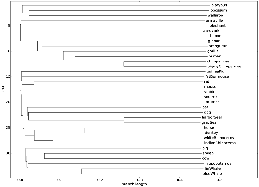
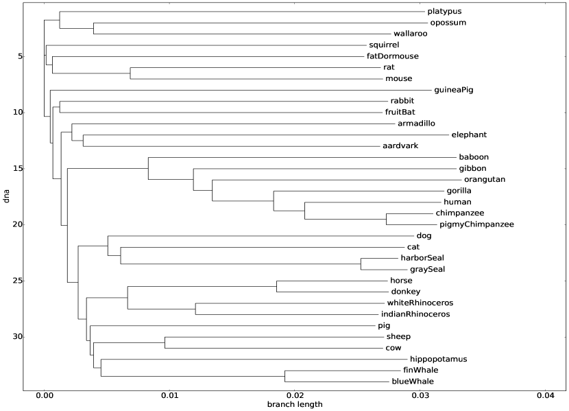
Figure 5: Mitochondrial DNA clustering with NCD/gzip (left) vs. NSD (right).

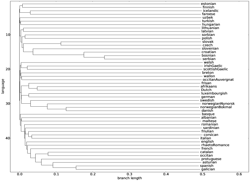
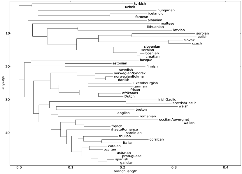
Figure 6: Clustering of writing systems (UDHR) using NCD/gzip (left) vs. NSD (right).

The effect of the first term in Eq. (6) is clear: the trees exhibit sharper clustering patterns than when using NCD/gzip, see Fig. (5–6). One has obviously a real advantage in taking into account the lengths produced by the SALZA factorization. This advantage seems even clearer when the data is more structured as it is the case with human writing systems.

It is remarkable that regarding the Basque language, NCD/gzip fails to group it with Finno-Ugric languages (Finnish and Estonian), which is one of the earliest hypotheses (XIX^th century) on the question of the origin of the Basque language ([20], Ch. 2). This hypothesis has been mostly rejected in the meantime. However, the stronger discriminative power of SALZA shows that this hypothesis could have seem plausible at some point in time. Because the branches of the phylogenic trees can be put upside-down without changing the meaning of the interpretation, an acute reader will see that the Basque language is also close to Altaic languages (Turkish, Uzbek), which count among other hypotheses that have been formulated in the past [20].

IV-A2 Synthetic data

As seen above, the phylogenic trees show sharper differences between clusters with SALZA. We now use several realizations of various first-order Markovian processes to compare with the NCD in the same setting. In the following plots, the data is labeled as alphaX_mY_cZ, where $\mbox{{X}}=|\mathcal{A}|$, Y is the identifier of the Markov transition probabilities matrix and Z is the identifier of the realization. Each realization string contains 15K literals (actually, bytes), so that we can fairly compare with NCD/gzip.

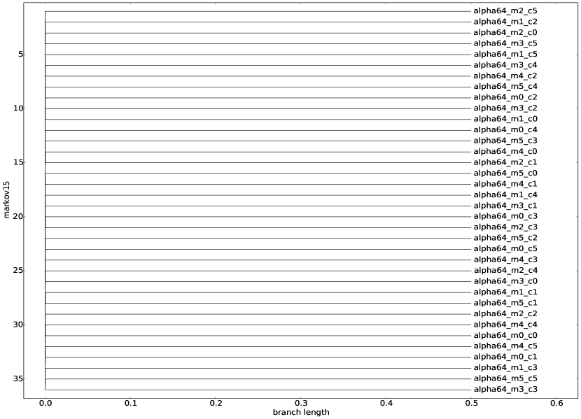
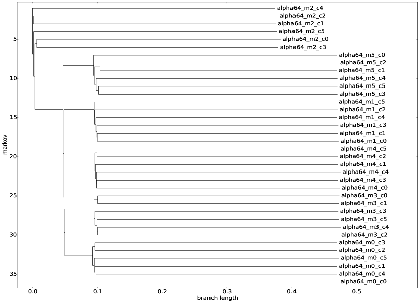
Figure 7: Clustering of Markovian processes using NCD/gzip (left) vs. NSD (right) – $|\mathcal{A}|=64$. The NCD/gzip mostly fails when SALZA succeeds in correctly clustering the Markovian processes with respect to their generative model.

Here, NCD/gzip is unable to correctly classify the realizations with respect to their Markov transition probabilities matrices – contrary to NSD, see Fig. (7). This further highlights the stronger discriminative power of NSD over NCD/gzip. The same results have been obtained using $|\mathcal{A}|=4$ or $|\mathcal{A}|=256$.

IV-A3 Larger data set

In order to produce meaningful results, the data at [14] is limited to chunks of 16KiB (so that the concatenation of two samples fits the gzip internal buffer length). Because we are now able to cluster data of arbitrary length, we use to this end a corpus of freely available French classical books in their entirety, see Fig. (8). Most books get classified by author and the branch lengths of the clusters are intuitively linked to the perception of a native French reader, thus confirming the cognitive nature of information distances.

Due to the internal, 32KiB limited length of gzip buffer [7], the NCD/gzip fails here as badly as in Fig. (7), hence we do not depicts these results to focus only on SALZA. The Neighbor-Joining method is known to sometimes produce negative branch lengths [18], this happens here for Montaigne. The unbounded buffer of SALZA allows to produce quite a meaningful classification of the books. Note that the tale genre gets classified as such (Perrault, Aulnoy), although the proper style of Voltaire makes his works a cluster of their own. SALZA roughly classifies books by author and by chronological order, thus reflecting the evolution of the French language itself.

Author	Work	Size
Montesquieu	De l’Esprit des Lois	2.1M
Dumas	Vingt Ans Après	1.7M
Rousseau	Les Confessions	1.6M
Dumas	Les Trois Mousquetaires	1.4M
Montaigne	Essais, II	1.2M
Stendhal	La Chartreuse de Parme	1.1M
Zola	Germinal	1.1M
Stendhal	Le Rouge et le Noir	1.1M
Zola	L’Assomoir	976K
Montaigne	Essais, III	886K
La Bruyère	Les Caractères	847K
Zola	La Bête Humaine	787K
Montaigne	Essais, I	764K
Sade	Justine	655K
Maupassant	Bel-Ami	644K
Aulnoy	Contes, I	634K
La Rochefoucauld	Maximes	616K
Rousseau	L’Émile (I–III)	586K
Pascal	Les Provinciales	573K
Montesquieu	Lettres Persanes	541K
Rousseau	L’Émile (IV)	486K
Aulnoy	Contes, 2	457K
Maupassant	Une Vie	451K
Maupassant	Fort Comme la Mort	439K
Montesquieu	Lettres Familières	390K
Maupassant	Mont Oriol	348K
Pascal	Pensées	341K
Montesquieu	Considérations	337K
Rabelais	Gargantua	298K
Sade	Les Infortunes de la Vertu	298K
Descartes	Élisabeth	290K
Voltaire	Roman et Contes	283K
Rabelais	Pantagruel	273K
Rousseau	Rêveries Prom. Solitaire	244K
Descartes	Les Passions de l’Âme	214K
Perrault	Contes	207K
Voltaire	Candide	194K
Descartes	Discours de la Méthode	126K
Zola	La Débâcle	123K

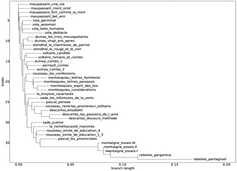
Figure 8: Clustering of French classic books ranging from XVI^th to XIX^th century (left) using the NSD.

IV-B Causality inference

Directed information is the tool of choice to perform causality inference. In this section, we illustrate the performance of the two different kinds of directed information we have defined above (Sec. III-B). In the first experiment, we concentrate on synthetic data to show how SALZA performs in a causal setting: we will recover the structure of several DAGs of random processes given one of their realizations. This is to simulate the behaviour of systems modeled by dependent time series. Here, we will naturally use Eq. (9).

In the second experiment, this time on real data, we will use SALZA to recover the order with which several versions of a text have been produced by an author. This will illustrate both the usefulness of full directed algorithmic information in Eq. (11) and the accuracy we obtain, even on a rather small data set.

IV-B1 Synthetic data

We have simulated DAGs of random processes using dependent processes: we have specified a connectivity matrix among processes whose weights are the probabilities of copying a string of length proportional to the said probability from the designated process. We also have a probability of generating random data.

Let $p_{n}$ ($0\leq n<N$) be random stationary processes over $\mathcal{A}$. The connectivity matrix $M\in\mathcal{M}_{N,N+1}\left(\left[0,1\right]\right)$ is such that:

$$\forall 0\leq i<N,\;\;\sum_{j=0}^{N}M_{i,j}=1,$$

the last column of $M$ being the probability of generating random, uniformly distributed symbols. This means that, for process $p_{i}$, the probability of copying data from any random point in the past of process $p_{j}$ is $M_{i,j}$ ($j<N$). If $j=N$ then we generate random, uniformly distributed data (the unobserved string that simulates the causal mechanism in the words of [21]). At each step, the length of the data being copied or generated is proportional to $M_{i,j}$. In order to initiate data generation, we have a short “burn-in” period of 12 symbols. The minimum length of data that is to be copied from the past of a process is three symbols (this is to ensure we can hook to the copied string, see footnote 1). As seen from Fig. (9), we are able to recover the structure of the DAGs.

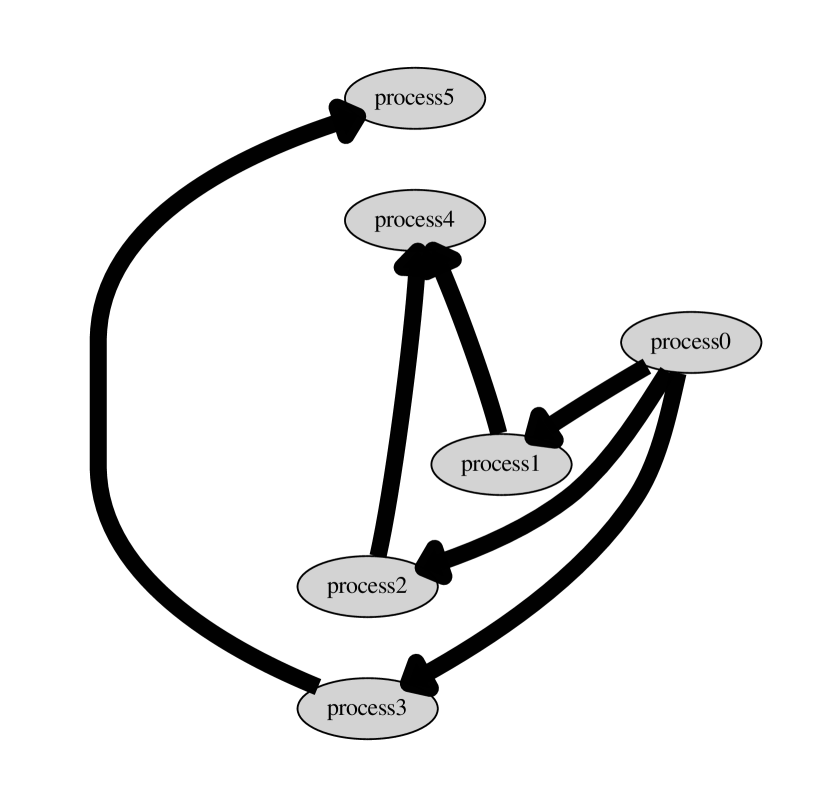
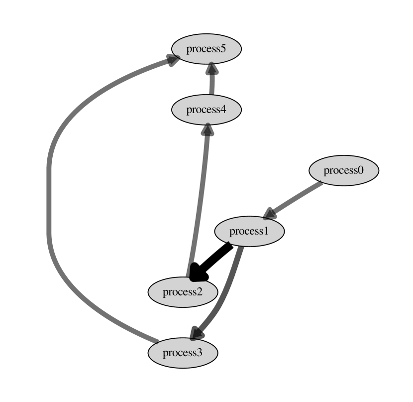
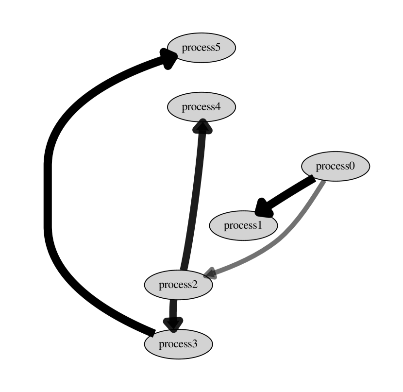
$M=$	$\left(\begin{array}[]{ccccccc}0&0&0&0&0&0&1.0\\ .50&0&0&0&0&0&.50\\ .50&0&0&0&0&0&.50\\ .50&0&0&0&0&0&.50\\ 0&.50&.50&0&0&0&0\\ 0&0&0&.50&0&0&.50\end{array}\right)$
	$\left(\begin{array}[]{cccccc}0&0&0&0&0&0\\ .60&0&0&0&0&0\\ .60&0&0&0&0&0\\ .60&0&0&0&0&0\\ 0&.02&.10&0&0&0\\ 0&0&0&.10&0&0\end{array}\right)$

$M=$	$\left(\begin{array}[]{ccccccc}00&0&0&0&0&0&1.0\\ .50&0&0&0&0&0&.50\\ 00&.90&0&0&0&0&.10\\ 00&.60&0&0&0&0&.40\\ 00&0&.50&0&0&0&.50\\ 00&0&0&.50&.50&0&0\end{array}\right)$
	$\left(\begin{array}[]{cccccc}0&0&0&0&0&0\\ .60&0&0&0&0&0\\ 0&.10&0&0&0&0\\ 0&.40&0&0&0&0\\ 0&0&.03&0&0&0\\ 0&0&0&.10&.04&0\end{array}\right)$

$M=$	$\left(\begin{array}[]{ccccccc}0&0&0&0&0&0&1.0\\ .90&0&0&0&0&0&.10\\ .50&0&0&0&0&0&.50\\ 0&0&.80&0&0&0&.20\\ 0&0&.80&0&0&0&.20\\ 0&0&0&.90&0&0&.10\end{array}\right)$
	$\left(\begin{array}[]{cccccc}0&0&0&0&0&0\\ .50&0&0&0&0&0\\ .40&0&0&0&0&0\\ 0&0&.30&0&0&0\\ 0&0&.30&0&0&0\\ 0&0&0&.10&0&0\end{array}\right)$

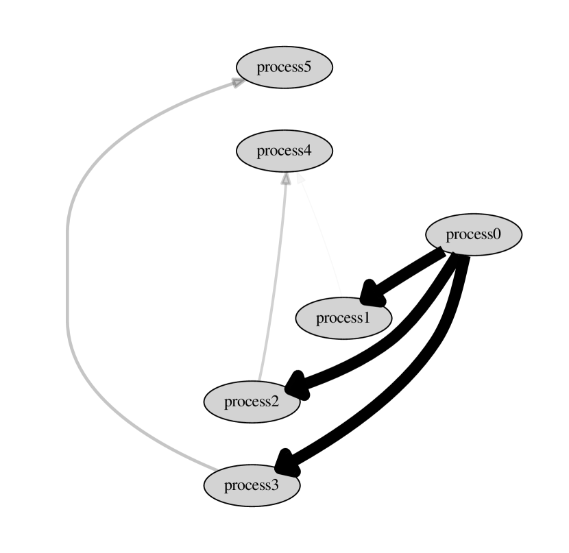
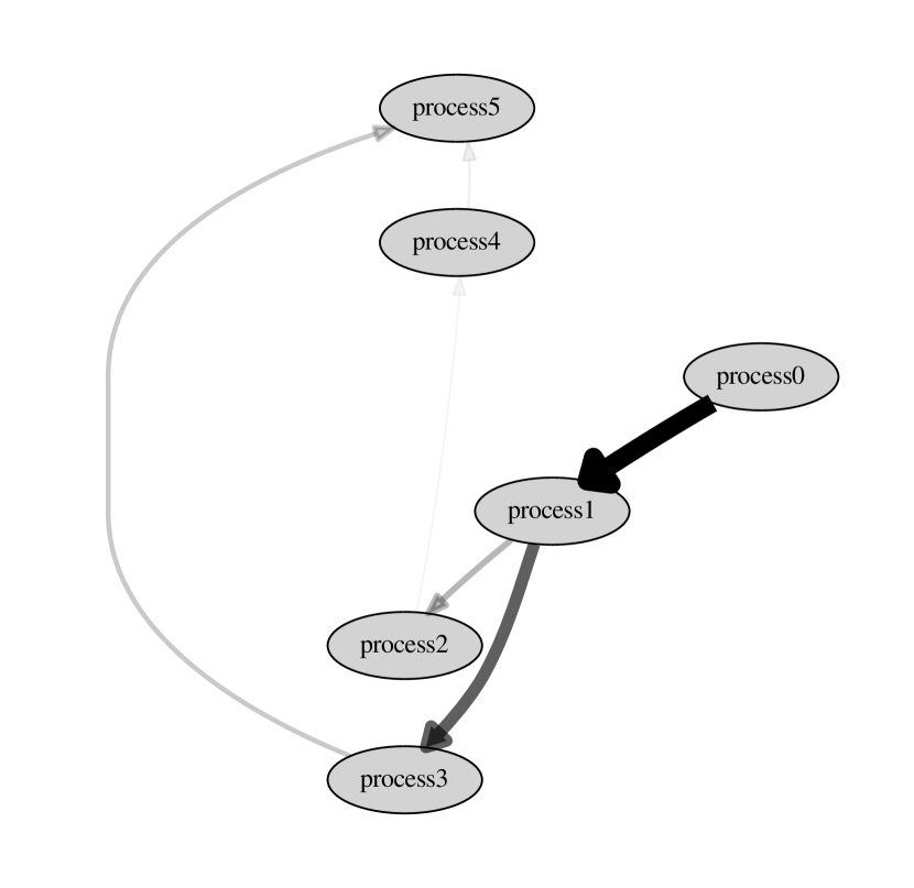
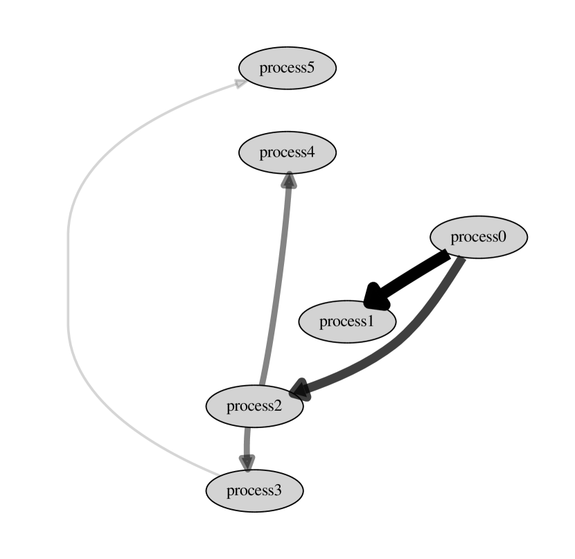
Figure 9: Top: Three sample target DAGs we want to recover from one of their realizations along with their connectivity matrix: the last column is the probability of creating random strings – this is the amount of innovation contained in the strings produced by the said process (and the source of randomness used to simulate innovation has not been represented for clarity). Bottom: Recovered connectivity matrices using $C_{S}$ along with their DAGs. We have filtered out directed information values such that $C_{S}(x_{i}\rightarrow x_{j})<5e-3$. Both the thickness and the transparency of the arrows are used to depict the amount of innovation created in one process and transmitted to another. This means that the structure of the DAG we are recovering is only dictated by the innovation created in every single process and transmitted to his neighbor(s). Some arrows may be faint to spot, but the recovered structure is correct in all cases.

IV-B2 An experiment in literature

Jean-Philippe Toussaint is a famous Belgian author of French expression with a specific way of writing: he works by producing paragraphs one after the other. Each paragraph gets typeset, annotated by hand, typeset again, annotated again, and so on until the author is satisfied. Some of his paragraphs culminate to more than 50 successive versions. In Fig. (10), we show the eight successive versions of one of his paragraphs (Jean-Philippe Toussaint does not necessarily typeset exactly the annotated version but makes changes in between). These versions are called fragments in Fig. (10) and Fig. (11). As one can see in top and middle plots of Fig. (11) (clustering using resp. Neighbor-Joining and UPGMA), our semi-distance allows to correctly recover the chronological order of the fragments. In this particular application, one would preferably use the UPGMA method because its results are more easily read into by non specialists.

On the lower graph of Fig. (11), all the arrows have been kept in order to allow in-depth inspection of the amount of differential innovation. This representation is certainly richer as it allows to grasp the amount of information that has been reused from one fragment to another. All three results allow to correctly recover the order with which the fragments have been actually written by Jean-Philippe Toussaint.

Figure 10: Draft scans of the last pages of Jean-Philippe Toussaint’s novel La Réticence [22], by the author (freely available at jptoussaint.com). The transcripts we have used are labeled as follows: Fragments 1 and 2 are the typeset and annotated versions of the upper-left scan, fragments 3 and 4 are the typeset and annotated versions of the upper-right scan, fragments 5 and 6 are the typeset and annotated versions of the lower-right scan, and fragments 7 and 8 are the typeset and annotated versions of the lower-left scan.

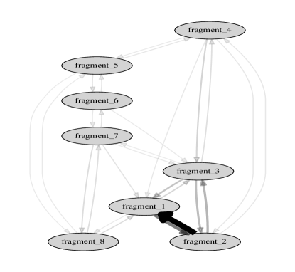
Figure 11: Top: The distance matrix of the data in Fig. (10) depicted using Neighbor-Joining [18] clustering (for the sake of completeness). Middle: The distance matrix depicted using UPGMA [19] clustering. This is the method of choice one would use in this case. Bottom: The inferred causality graph using $F_{S}$ (because the author may have – actually, has – moved parts of the fragments later in the text).

References

- [1] M. Li, X. Chen, X. Li, B. Ma, and P. M. Vitányi, “The Similarity Metric,” IEEE Transactions on Information Theory, vol. 50, pp. 3250–3264, Dec. 2004. [Online]. Available: http://dx.doi.org/10.1109/tit.2004.838101
- [2] M. Li and P. M. Vitániy, An Introduction to Kolmogorov Complexity and Its Applications. Springer-Verlag New-York, 2008. [Online]. Available: http://dx.doi.org/10.1007/978-0-387-49820-1
- [3] L.-Y. Zhang and C.-X. Zheng, “Analysis of Kolmogorov Complexity in Spontaneous EEG Signals and Its Appliction to Assessment of Mental Fatigue,” 2008, pp. 2192–2194. [Online]. Available: http://dx.doi.org/10.1109/ICBBE.2008.878
- [4] A. Petrosian, “Kolmogorov Complexity of Finite Sequences and Recognition of Different Preictal EEG Patterns,” 1995, pp. 212–217. [Online]. Available: http://dx.doi.org/10.1109/CBMS.1995.465426
- [5] R. Cilibrasi and P. M. Vitányi, “Clustering by Compression,” IEEE Transactions on Information Theory, vol. 51, pp. 1523–1545, Apr. 2005. [Online]. Available: http://dx.doi.org/10.1109/tit.2005.844059
- [6] A. Lempel and J. Ziv, “On the Complexity of Finite Sequences,” IEEE Transactions on Information Theory, vol. 22, pp. 75–81, January 1976. [Online]. Available: http://dx.doi.org/10.1109/tit.1976.1055501
- [7] M. Cebrián, M. Alfonseca, and A. Ortega, “Common Pitfalls Using the Normalized Compression Distance: What to Watch Out for in a Compressor,” Communications in Information and Systems, vol. 5, pp. 367–384, 2005. [Online]. Available: http://dx.doi.org/10.4310/cis.2005.v5.n4.a1
- [8] C. H. Bennett, P. Gacs, M. Li, P. M. Vitániy, and W. H. Zurek, “Information Distance,” IEEE Transactions on Information Theory, vol. 44, pp. 1407–1423, Jul. 1998. [Online]. Available: http://dx.doi.org/10.1109/18.681318
- [9] J. Ziv and A. Lempel, “A Universal Algorithm for Sequential Data Compression,” IEEE Transactions on Information Theory, vol. 23, pp. 337–343, May 1977. [Online]. Available: http://dx.doi.org/10.1109/tit.1977.1055714
- [10] L. P. Deutsch, “DEFLATE Compressed Data Format Specification, version 1.3,” 1996. [Online]. Available: http://www.gzip.org/zlib/rfc-deflate.html
- [11] I. Pavlov, “7z Format.”
- [12] J. Ziv and N. Merhav, “A Measure of Relative Entropy Between Individual Sequences with Application to Universal Classification,” IEEE Transactions on Information Theory, vol. 39, pp. 1270–1279, Jul. 1993. [Online]. Available: http://dx.doi.org/10.1109/isit.1993.748668
- [13] A. Silverstein, “Judy IV Shop Manual,” Jan. 2002. [Online]. Available: http://judy.sourceforge.net/application/shop_interm.pdf
- [14] R. Cilibrasi, A. L. Cruz, S. de Rooij, and M. Keijzer, “CompLearn,” 2008. [Online]. Available: http://complearn.org
- [15] J. Pearl, Causality, Models, Reasoning, and Inference. Cambridge University Press, 2009. [Online]. Available: http://dx.doi.org/10.1017/cbo9780511803161
- [16] C. W. Granger, “Investigating Causal Relations by Econometric Models and Cross-spectral Methods,” Econometrica, vol. 37, pp. 424–438, Aug. 1969. [Online]. Available: https://dx.doi.org/10.2307/1912791
- [17] P.-O. Amblard and O. Michel, “The Relation between Granger Causality and Directed Information Theory: A Review,” Entropy, vol. 15, pp. 113–143, 2013. [Online]. Available: http://dx.doi.org/10.3390/e15010113
- [18] N. Saitou and M. Nei, “The Neighbor-Joining Method: A New Method for Reconstructing Phylogenic Trees,” Molecular Biology and Evolution, vol. 4, pp. 406–425, July 1987.
- [19] R. Sokal and C. Michener, “A Statistical Method for Evaluating Systematic Relationships,” The University of Kansas Scientific Bulletin, vol. 38, pp. 1409–1438, March 1958.
- [20] M. Morvan, “Les Origines Linguistiques du Basque : L’Ouralo-Altaïque,” Ph.D. dissertation, Université de Bordeaux 3, Presses Universitaires de Bordeaux, 1992, in French.
- [21] D. Janzing and B. Schölkopf, “Causal Inference Using the Algorithmic Markov Condition,” IEEE Transactions on Information Theory, vol. 56, pp. 5168–5194, Oct. 2010. [Online]. Available: http://dx.doi.org/10.1109/TIT.2010.2060095
- [22] J.-P. Toussaint, La Réticence. Les Éditions de Minuit, 1991. [Online]. Available: http://www.leseditionsdeminuit.fr/livre-La_R%C3%A9ticence-1878-1-1-0-1.html