Cell averaging two-scale convergence
Applications to periodic homogenization

Abstract

The aim of the paper is to introduce an alternative notion of two-scale convergence which gives a more natural modeling approach to the homogenization of partial differential equations with periodically oscillating coefficients: while removing the bother of the admissibility of test functions, it nevertheless simplifies the proof of all the standard compactness results which made classical two-scale convergence very worthy of interest: bounded sequences in $L^{2}_{\sharp}[Y,L^{2}(\Omega)]$ and $L^{2}_{\sharp}[Y,H^{1}(\Omega)]$ are proven to be relatively compact with respect to this new type of convergence. The strengths of the notion are highlighted on the classical homogenization problem of linear second-order elliptic equations for which first order boundary corrector-type results are also established. Eventually, possible weaknesses of the method are pointed out on a nonlinear problem: the weak two-scale compactness result for $\mathbf{S}^{2}$-valued stationary harmonic maps.

A.M.S. subject classification: 35B27, 35B40, 74Q05

Keywords: periodic homogenization, two-scale convergence, boundary layers, cell averaging, multiscale problems

1 Introduction and Motivations

The aim of the paper is to study a new notion of two-scale convergence which is very natural and, in our opinion, gives a more straightforward approach to the homogenization process: while removing the bother of the admissibility of test functions [1, 12], it nevertheless simplifies the proof of all standard compactness results which made classical two-scale convergence (introduced in [14, 1]) very worthy of interest.

Attempts to overcome the question of admissibility of test functions arising in the definition of two-scale convergence have been the subject of various authors [6, 13, 17]. Among them, the periodic unfolding method is considered one of the most successful. The idea, as well as its nomenclature, is introduced [6] where the authors exploit a natural, although purely mathematical, intuition to recover two-scale convergence as a classical functional weak convergence in a suitable larger space. This recovery process is achieved by introducing the so-called unfolding operator which, roughly speaking, turns a sequence of $1$-scale functions into a sequence of $2$-scale functions.

On the other hand, as it is simple to show by playing with Lebesgue differentiation theorem, the recovery process is not univocal, and many alternatives are possible. In guessing the one presented below, we did not rely on mathematical intuition only, but we found inspiration from the physics of the homogenization process. That is why we think it is important to dwell on some preliminary considerations before giving definitions, theorems and proofs.

The paper is organized as follows: in Section 2 we explain the idea behind the proposed approach which will be formalized in Section 3. In Section 4 we establish compactness results for the new notion of two-scale convergence which play a central role in the homogenization process. In Section 5 we test the effectiveness of our notion of convergence on the «classical» model problem in the theory of homogenization, i.e the one associate to a family of linear second-order elliptic partial differential equation with periodically oscillating coefficients. Section 6 is devoted to the so-called first-order corrector results which aim to improve the convergence of the solution gradients by adding corrector term. In Section 7 we introduce the well-known boundary layer terms which aim to compensate the fast oscillation of the family of solutions near the boundary. Eventually, in Section 8 we test the approach on a nonlinear problem: we prove a weak two-scale compactness result for $\mathbf{S}^{2}$-valued stationary harmonic map, and make some remarks which point out some possible weaknesses of this alternative notion of two-scale convergence.

2 The cell averaging approach to periodic homogenization

2.1 The classical two-scale convergence approach to periodic homogenization

Let us focus on the classical model problem in homogenization: a linear second-order partial differential equation with periodically oscillating coefficients. Such an equations models, for example, the stationary heat conduction in a periodic composite medium [1, 7]. We denote by $\Omega$ the material domain (a bounded open set in $\mathbb{R}^{N}$) and by $Y:=[0,1]^{N}$ the unit cell of $\mathbb{R}^{N}$. Denoting by $f\in L^{2}(\Omega)$ the source term and enforcing a Dirichlet boundary condition for the unknown $u_{\varepsilon}$, the model equation reads as

$$-\operatorname{div}(A_{\varepsilon}\nabla u_{\varepsilon})=f\quad\text{in }\Omega,\quad u_{\varepsilon}=0\quad\text{on }\partial\Omega,$$ (1)

where, for any $\varepsilon>0$, we have defined $A_{\varepsilon}$ by $A_{\varepsilon}(x):=A(x/\varepsilon)$, with $A$ (the so-called matrix of diffusion coefficients) an $L^{\infty}$ and $Y$-periodic matrix valued function, which is uniformly coercive, i.e. such that for two positive constants $0<\alpha\leqslant\beta$ one has (for a.e. $y\in Y$) $\alpha|\xi|^{2}\leqslant A(y)\xi\cdot\xi\leqslant\beta|\xi|^{2}$ for every $\xi\in\mathbb{R}^{N}$. Here we have supposed $A$ depending on the periodic variable only although later we will work with the more general case in which $A$ depends on the $x$ variable too. The weak formulation of problem (1) reads as:

$$\int_{\Omega}A_{\varepsilon}\nabla u_{\varepsilon}\cdot\nabla\varphi=\int_{\Omega}f\varphi,$$ (2)

and according to Lax-Milgram theorem for each $\varepsilon>0$ there exists a unique weak solution $u_{\varepsilon}\in H_{0}^{1}(\Omega)$ of (2). The family of solutions $(u_{\varepsilon})_{{}_{\varepsilon\in\mathbb{R}^{+}}}$ and the family of fluxes $(\xi_{\varepsilon})_{\varepsilon\in\mathbb{R}^{+}}:=(A_{\varepsilon}\nabla u_{\varepsilon})_{\varepsilon\in\mathbb{R}^{+}}$, constitute bounded subsets respectively of $H_{0}^{1}(\Omega)$ and $L^{2}(\Omega)$. Thus there exist subfamilies (that we still denote by $(u_{\varepsilon})_{\varepsilon\in\mathbb{R}^{+}}$ and $(\xi_{\varepsilon})_{\varepsilon\in\mathbb{R}^{+}}$) and elements $u_{0}\in H_{0}^{1}(\Omega),\xi_{0}\in L^{2}(\Omega)$ such that $\nabla u_{\varepsilon}\rightharpoonup\nabla u_{0}$ and $\xi_{\varepsilon}\rightharpoonup\xi_{0}$ weakly in $L^{2}(\Omega)$. Hence, passing to the limit in (2), we get $(\xi_{0},\nabla\varphi)_{L^{2}(\Omega)}=(f,\varphi)_{L^{2}(\Omega)}$, where the limit flux $\xi_{0}$ is the weak limit of the product of the weakly convergent sequences $\nabla u_{\varepsilon}\rightharpoonup\nabla u_{0}$ and $A_{\varepsilon}\rightharpoonup\langle A\rangle_{Y}$. The identification of the limit flux $\xi_{0}$ in terms of $u_{0}$ and $A$ is the first aim in the mathematical theory of periodic homogenization.

A procedure for the homogenization of problem (1) appeared in 1989 by the means of the so-called two-scale convergence. This notion, introduced for the first time by Nguetseng in [14], was later named «two-scale convergence» by Allaire [1] who further developed the notion by giving more direct proofs of the main compactness results. To better understand the idea behind the classical two-scale approach, let us recall the following compactness results [1], from which the notion of two-scale convergence originates:

Proposition 1 (Nguetseng [14], Allaire [1])

If $(u_{\varepsilon})_{\varepsilon\in\mathbb{R}^{+}}$ is a bounded sequence in $L^{2}(\Omega)$, there exists $u_{0}\in L^{2}\left(\Omega\times Y\right)$, such that, up to a subsequence

$$\lim_{\varepsilon\rightarrow 0}\int_{\Omega}u_{\varepsilon}(x)\varphi(x,x/\varepsilon)\mathrm{d}x=\int_{\Omega\times Y}u_{0}(x,y)\varphi(x,y)\mathrm{d}x\;\mathrm{d}y$$ (3)

for any test function $\varphi\in\mathcal{D}[\Omega,C^{\infty}_{\sharp}\left(Y\right)]$. Moreover, if $(u_{\varepsilon})_{\varepsilon\in\mathbb{R}^{+}}$ is a bounded sequence in $H^{1}(\Omega)$, then there exist functions $u_{0}\in H^{1}(\Omega)$ and $u_{1}\in L^{2}[\Omega,H^{1}_{\sharp}\left(Y\right)/\mathbb{R}]$ such that, up to a subsequence

$$\lim_{\varepsilon\rightarrow 0}\int_{\Omega}\nabla u_{\varepsilon}(x)\cdot\psi(x,x/\varepsilon)\mathrm{d}x=\int_{\Omega\times Y}\left(\nabla_{x}u_{0}(x)+\nabla_{y}u_{1}(x,y)\right)\cdot\psi(x,y)\mathrm{d}x\;\mathrm{d}y$$ (4)

for any test function $\psi\in\mathcal{D}[\Omega,C^{\infty}_{\sharp}\left(Y\right)]^{N}$.

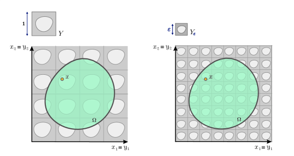
Figure 1: If we assume that the heterogeneities are evenly distributed inside the media $\Omega$, we can model the material as periodic. As illustrated in the figure, this means that we can think of the material as being immersed in a grid of small identical cubes $Y_{\varepsilon}$, the side-length of which is $\varepsilon$.

It is then natural to give the following (see [1])

Definition 1 (Allaire [1])

A sequence of functions $u_{\varepsilon}$ in $L^{2}(\Omega)$ two-scale converges to a limit $u_{0}\in L^{2}\left(\Omega\times Y\right)$ if, for any function $\varphi\in\mathcal{D}[\Omega,C^{\infty}_{\sharp}\left(Y\right)]$ we have

$$\lim_{\varepsilon\rightarrow 0}\int_{\Omega}u_{\varepsilon}(x)\varphi(x,x/\varepsilon)\mathrm{d}x=\int_{\Omega\times Y}u_{0}(x,y)\varphi(x,y)\mathrm{d}x\;\mathrm{d}y.$$ (5)

In that case we write $u_{\varepsilon}\xrightarrow{2s}u_{0}$. We say that the sequence $(u_{\varepsilon})$ strongly two-scale converges to a limit $u_{0}\in L^{2}\left(\Omega\times Y\right)$, if $u_{\varepsilon}\xrightarrow{2s}u_{0}$ and $\|u_{0}\|_{L^{2}\left(\Omega\times Y\right)}=\lim_{\varepsilon\rightarrow 0}\|u_{\varepsilon}\|_{L^{2}(\Omega)}$.

It is now immediate to understand the role played by two-scale convergence in the homogenization process. Indeed, by writing (2) in the form

$$\int_{\Omega}\nabla u_{\varepsilon}(x)\cdot A^{\mathsf{T}}\left(\frac{x}{\varepsilon}\right)\nabla\varphi_{\varepsilon}(x)\mathrm{d}x\;=\;\int_{\Omega}f(x)\varphi_{\varepsilon}(x)\mathrm{d}x,$$ (6)

and choosing the right shape for the test functions $\varphi_{\varepsilon}$, it is possible to interpret the left-hand side of the previous relation as the product of a strongly two-scale convergent sequence (namely $A^{\mathsf{T}}_{\varepsilon}\nabla\varphi_{\varepsilon}(x)$) with the weakly two-scale convergent sequence $\nabla u_{\varepsilon}$, from which weak two-scale convergence of the product, and hence the homogenized equation, easily follows (cfr. [1, 7] for details).

Unfortunately, for this procedure to be possible it is essential to add a technical hypothesis: the sequence of coefficients $(A_{\varepsilon})$ must be admissible in the sense that (cfr. [1])

$$\lim_{\varepsilon\rightarrow 0}\|A_{\varepsilon}\|_{L^{2}(\Omega)}\;=\;\|A\|_{L^{2}\left(\Omega\times Y\right)}.$$ (7)

It turns out that this is a subtle notion. Indeed, for a given function $\psi\in L^{2}_{\sharp}[Y,L^{2}(\Omega)]$ there is no reasonable way to give a meaning to the «trace» function $x\mapsto\psi(x,x/\varepsilon)$. The complete space of admissible functions is not known much more precisely. Functions in $L^{p}[\Omega,C_{\sharp}\left(Y\right)]$ as well as $L^{p}_{\sharp}[Y,C(\Omega)]$ are admissible, but it is unclear how much the regularity of $\psi$ can be weakened: we refer to [1] for an explicit construction of a non admissible function which belongs to $C[\Omega,L^{1}_{\sharp}\left(Y\right)]$.

2.2 The cell averaging idea

The «classical» approach to periodic homogenization originates by the modeling assumption that since the heterogeneities are evenly distributed inside the media $\Omega$, we can think of the material as being immersed in a grid of small identical cubes $Y_{\varepsilon}$, the side-length of which is $\varepsilon$ (see Figure 1). If we denote by $\Omega_{a}:=\Omega+a$, with $a\in\mathbb{R}^{N}$, a translated copy of $\Omega$ such that $\Omega\cap\Omega_{a}\neq\emptyset$, this modeling approach assumes that, at scale $\varepsilon$, the contribution of the diffusion coefficients at any $x\in\Omega\cap\Omega_{a}$, is given by $A(x/\varepsilon)$ both if we focus on the problem $-\operatorname{div}(A_{\varepsilon}\nabla u_{\varepsilon})=f$ in $\Omega$ and on the problem $(f_{a}:=f(x-a))$ $-\operatorname{div}(A_{\varepsilon}\nabla u_{\varepsilon})=f_{a}$ in $\Omega_{a}$. Although this assumption is mathematically reasonable when $\varepsilon$ tends to be very small, it is nevertheless the reason why the two-scale convergence produces «two-variables» functions starting from a family of «one-variable» functions.

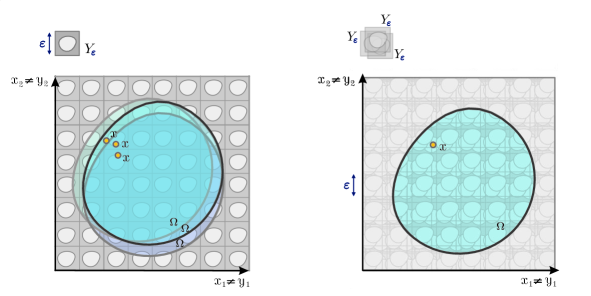
Figure 2: More realistic is to think of the material as being immersed in a grid of small identical cubes $Y_{\varepsilon}$, up to an unknown translation of size smaller than $\varepsilon$. We thus consider all possible translations, which we take into account by the introduction of a new variable.

On the other hand, it is clear that a more realistic approach consists in taking into account the effects of the diffusion coefficients $A_{\varepsilon}:=A(x/\varepsilon)$ via a family of displacement of length at most $\varepsilon$, i.e. via the family of diffusion coefficients $\left(A_{\varepsilon}\left(\,\cdot\,+\varepsilon y\right)\right)_{(\varepsilon,y)\in\mathbb{R}^{+}\times Y}=(A(y+\cdot/\varepsilon))_{(\varepsilon,y)\in\mathbb{R}^{+}\times Y}$, and hence (see Figure 2) via the family of boundary value problems depending on the cell-size parameter $\varepsilon\in\mathbb{R}^{+}$ and on the translation parameter $y\in Y$. The new homogenized problem then goes through the following two steps: for every $\varepsilon\in\mathbb{R}^{+}$ find (in a suitable sense) a $Y$-periodic solution $u_{\varepsilon}(x,y)$ of the Dirichlet problem

$$-\operatorname{div}(A_{\varepsilon}(x+\varepsilon y)\nabla u_{\varepsilon}(x,y))=f(x)\quad\text{in }\Omega,\quad u_{\varepsilon}(x,y)=0\quad\text{on }\partial\Omega;$$ (8)

then take the average $\langle u_{\varepsilon}\rangle_{Y}$ as a more realistic modelization of the solution associated, at scale $\varepsilon$, to evenly distributed heterogeneities inside the media $\Omega$.

In this framework the homogenization process demands for the computation of the limiting behaviour, as $\varepsilon\rightarrow 0$, of the family of two variable solutions $u_{\varepsilon}(x,y)$, i.e. for an asymptotic expansion of the form

$$u_{\varepsilon}(x,y)\;=\;u_{0}\left(x,y+\frac{x}{\varepsilon}\right)+\varepsilon\;u_{1}\left(x,y+\frac{x}{\varepsilon}\right)+\varepsilon^{2}\;u_{2}\left(x,y+\frac{x}{\varepsilon}\right)+\cdots,$$ (9)

in which $u_{0}$ is the solution of the homogenized equation and $u_{1}$ is the so-called first order corrector (cfr. the analogues definitions in [1, 7]).

We are now in position to explain the new approach. To this end, let us introduce the operator

$$\mathcal{F}_{\varepsilon}:u\in L^{2}_{\sharp}[Y,L^{2}(\Omega)]\mapsto u(x,y-x/\varepsilon)\in L^{2}_{\sharp}[Y,L^{2}(\Omega)].$$ (10)

Due to the $Y$-periodicity of $A$, the variational formulation of (8) reads as the problem of finding $u_{\varepsilon}\in L^{2}_{\sharp}[Y,H^{1}_{0}(\Omega)]$ such that

$$\int_{\Omega\times Y}A(y)\mathcal{F}_{\varepsilon}\left(\nabla_{x}u_{\varepsilon}\right)(x,y)\cdot\mathcal{F}_{\varepsilon}\left(\nabla_{x}\psi_{\varepsilon}\right)(x,y)\mathrm{d}x\mathrm{d}y\;=\;\int_{\Omega\times Y}f(x)\mathcal{F}_{\varepsilon}(\psi_{\varepsilon})(x,y)\mathrm{d}x\mathrm{d}y$$ (11)

for every $\psi_{\varepsilon}\in L^{2}_{\sharp}[Y,H^{1}_{0}(\Omega)]$. Therefore, if $\mathcal{F}_{\varepsilon}\left(\nabla_{x}u_{\varepsilon}\right)\rightharpoonup\boldsymbol{v}$ weakly in $L^{2}_{\sharp}[Y,L^{2}(\Omega)]$, then for every couple of «test functions» $\psi,\boldsymbol{\psi}\in L^{2}_{\sharp}[Y,L^{2}(\Omega)]$ such that for some family $\psi_{\varepsilon}\in L^{2}_{\sharp}[Y,H^{1}_{0}(\Omega)]$ we have $\mathcal{F}_{\varepsilon}(\psi_{\varepsilon})\rightarrow\psi$ and $\mathcal{F}_{\varepsilon}\left(\nabla_{x}\psi_{\varepsilon}\right)\rightarrow\boldsymbol{\psi}$ strongly in $L^{2}_{\sharp}[Y,L^{2}(\Omega)]$, passing to the limit in (11), we finish with the «homogenized equation»

$$\int_{\Omega\times Y}A(y)\boldsymbol{v}(x,y)\cdot\boldsymbol{\psi}(x,y)\mathrm{d}x\mathrm{d}y\;=\;\int_{\Omega\times Y}f(x)\psi(x,y)\mathrm{d}x\mathrm{d}y.$$ (12)

Of course, to find an explicit expression for the homogenized equation, and more generally to build a kind of two-scale calculus, it is important to investigate the interconnections between the convergence of the families $u_{\varepsilon}$ and $\mathcal{F}_{\varepsilon}(u_{\varepsilon})$ in $L^{2}_{\sharp}[Y,H^{1}(\Omega)]$, and to understand which are the subspaces of $L^{2}_{\sharp}[Y,H^{1}(\Omega)]$ which are reachable by strong convergence of family of the type $\mathcal{F}_{\varepsilon}(\varphi_{\varepsilon})$ in $L^{2}_{\sharp}[Y,H^{1}(\Omega)]$. This and many other important aspects of the question are the object of the next two sections.

3 The alternative approach to two-scale convergence

3.1 Notation and preliminary definitions

In what follows we denote by $Y=[0,1]^{N}$ the unit cell of $\mathbb{R}^{N}$ and by $\Omega$ an open set of $\mathbb{R}^{N}$. For any measurable function $u$ defined on $Y$ we denote by $\langle u\rangle_{Y}$ the integral average of $u$.

By $C^{\infty}_{\sharp}[Y,\mathcal{D}(\Omega)]$ we mean the vector space of test functions $u:\Omega\times\mathbb{R}^{N}\rightarrow\mathbb{R}$ such that the section $u(x,\cdot)\in C^{\infty}_{\sharp}\left(Y\right)$ for every $x\in\Omega$, and the section $u(\cdot,y)\in\mathcal{D}(\Omega)$ for every $y\in\mathbb{R}^{N}$. Similarly we denote by $L^{2}_{\sharp}[Y,L^{2}(\Omega)]$ the Hilbert space of $Y$-periodic distributions which are in $L^{2}\left(\Omega\times Y\right)$, and by $L^{2}_{\sharp}[Y,H^{1}(\Omega)]$ the Hilbert subspace of $L^{2}_{\sharp}[Y,L^{2}(\Omega)]$ constituted of distributions $u$ such that $\nabla_{x}u\in L^{2}_{\sharp}[Y,L^{2}(\Omega)]$.

Next, we denote by $L^{2}[\Omega;H^{1}_{\sharp}\left(Y\right)]$ the Hilbert space of $Y$-periodic distributions $u\in\mathcal{D}^{\prime}\left(\Omega\times\mathbb{R}^{N}\right)$ such that $u(\cdot,y)\in L^{2}(\Omega)$ for a.e. $y\in Y$ and $u(x,\cdot)\in H^{1}_{\operatorname{loc}}\left(\mathbb{R}^{N}\right)$ for a.e. $x\in\Omega$.

Finally, in the next Proposition 2, we denote by $\mathcal{E}^{\prime}_{\sharp}[Y,\mathcal{D}^{\prime}(\Omega)]$ the algebraic dual of $C^{\infty}_{\sharp}[Y,\mathcal{D}(\Omega)]$, and for any $u\in\mathcal{E}^{\prime}_{\sharp}[Y,\mathcal{D}^{\prime}(\Omega)]$ and any $\boldsymbol{\psi}\in C^{\infty}_{\sharp}[Y,\mathcal{D}(\Omega)]^{N}$ we define the partial gradient $\nabla_{x}u$ by the position $\left\langle\nabla_{x}u,\boldsymbol{\psi}\right\rangle:=-\left\langle u,\operatorname{div}_{x}\boldsymbol{\psi}\right\rangle$ and the $\varepsilon$-cell shifting of $u$ by the position $\langle u(x,y-x/\varepsilon),\boldsymbol{\psi}(x,y)\rangle:=\langle u(x,y),\boldsymbol{\psi}(x,y+x/\varepsilon)\rangle$.

3.2 Cell averaging two-scale convergence

Motivated by the considerations made in subsection 2.2 we give the following

Definition 2

Let $\Omega\subseteq\mathbb{R}^{N}$ be an open set and $Y$ the unit cell of $\mathbb{R}^{N}$. For any $\varepsilon>0$, we define the $\varepsilon$-cell shift operator $\mathcal{F}_{\varepsilon}$ by the position

$$u\in L^{2}_{\sharp}[Y,L^{2}(\Omega)]\mapsto\mathcal{F}_{\varepsilon}(u):=u(x,y-x/\varepsilon)\in L^{2}_{\sharp}[Y,L^{2}(\Omega)],$$ (13)

i.e. as the composition of $u$ with the diffeomorphism $(x,y)\in\Omega\times\mathbb{R}^{N}\mapsto(x,y-x/\varepsilon)\in\Omega\times\mathbb{R}^{N}$. We then denote by $\mathcal{F}^{\ast}_{\varepsilon}$ the algebraic adjoint operator which maps $u(x,y)$ to $u(x,y+x/\varepsilon)$.

Definition 3

A sequence of $L^{2}_{\sharp}[Y,L^{2}(\Omega)]$ functions $(u_{\varepsilon})_{\varepsilon\in\mathbb{R}^{+}}$ is said to weakly two-scale converges to a function $u_{0}\in L^{2}_{\sharp}[Y,L^{2}(\Omega)]$, if $\mathcal{F}_{\varepsilon}(u_{\varepsilon})\rightharpoonup u_{0}$ weakly in $L^{2}_{\sharp}[Y,L^{2}(\Omega)]$, i.e if and only if

$$\lim_{\varepsilon\rightarrow 0^{+}}\int_{\Omega\times Y}u_{\varepsilon}\left(x,y-\frac{x}{\varepsilon}\right)\psi(x,y)\mathrm{d}x\mathrm{d}y=\int_{\Omega\times Y}u_{0}(x,y)\psi(x,y)\mathrm{d}x\mathrm{d}y,$$ (14)

for every $\psi\in L^{2}_{\#}[Y,L^{2}(\Omega)]$. In that case we write $u_{\varepsilon}\twoheadrightarrow u_{0}$ weakly in $L^{2}_{\sharp}[Y,L^{2}(\Omega)]$. We say that $u_{\varepsilon}\twoheadrightarrow u_{0}$ strongly in $L^{2}_{\sharp}[Y,L^{2}(\Omega)]$ if $\mathcal{F}_{\varepsilon}(u_{\varepsilon})\rightarrow u_{0}$ strongly in $L^{2}_{\sharp}[Y,L^{2}(\Omega)]$.

Remark 1

We have stated the definition in the framework of square summable functions. Nevertheless, almost all of what we say here and hereinafter easily extends, with obvious modifications, to the setting of $L^{p}$ spaces.

Remark 2

Since the notion of two-scale convergence relies on the classical notion of weak convergence in Banach space, we immediately get, among others, boundedness in norm of weakly two-scale convergent sequences. This aspect is not captured by the classical notion of two-scale convergence which, by testing convergence on functions in $\mathcal{D}[\Omega,C^{\infty}_{\sharp}\left(Y\right)]$, i.e. having compact support in $\Omega$, may cause loss of information on any concentration of «mass» near the boundary of the sequence $(u_{\varepsilon})_{\varepsilon\in\mathbb{R}^{+}}$ (cfr. [12]).

We now state some properties of the operator $\mathcal{F}_{\varepsilon}$, which are simple consequence of the definitions, and will be used extensively (and sometime tacitly) in the sequel:

Proposition 2

Let $\varepsilon>0$. The operator $\mathcal{F}_{\varepsilon}$ is an isometric isomorphism of $L^{2}_{\sharp}[Y,L^{2}(\Omega)]$ and the following relations hold:

• If $\boldsymbol{\psi}\in C^{\infty}_{\sharp}[Y,\mathcal{D}(\Omega)]^{N}$ then $\mathcal{F}_{\varepsilon}(\boldsymbol{\psi})\in C^{\infty}_{\sharp}[Y,\mathcal{D}(\Omega)]^{N}$ and one has

  $$\operatorname{div}_{x}\mathcal{F}_{\varepsilon}(\boldsymbol{\psi})=\mathcal{F}_{\varepsilon}\left(\operatorname{div}_{x}\boldsymbol{\psi}\right)-\frac{1}{\varepsilon}\mathcal{F}_{\varepsilon}\left(\operatorname{div}_{y}\boldsymbol{\psi}\right),\quad\operatorname{div}_{y}\mathcal{F}_{\varepsilon}(\boldsymbol{\psi})=\mathcal{F}_{\varepsilon}\left(\operatorname{div}_{y}\boldsymbol{\psi}\right).$$ (15)

Next, let us denote by $\mathcal{E}^{\prime}_{\sharp}[Y,\mathcal{D}^{\prime}(\Omega)]$ the algebraic dual of $C^{\infty}_{\sharp}[Y,\mathcal{D}(\Omega)]$:

• If $u\in\mathcal{E}^{\prime}_{\sharp}[Y,\mathcal{D}^{\prime}(\Omega)]$ then $\mathcal{F}_{\varepsilon}(u)\in\mathcal{E}^{\prime}_{\sharp}[Y,\mathcal{D}^{\prime}(\Omega)]$ and one has

  $$\left\langle\nabla_{x}[\mathcal{F}_{\varepsilon}(u)],\boldsymbol{\psi}\right\rangle=\left\langle\mathcal{F}_{\varepsilon}\left(\nabla_{x}u\right)-\frac{1}{\varepsilon}\mathcal{F}_{\varepsilon}\left(\nabla_{y}u\right),\boldsymbol{\psi}\right\rangle,\quad\left\langle\mathcal{F}_{\varepsilon}\left(\nabla_{y}u\right),\boldsymbol{\psi}\right\rangle=\left\langle\nabla_{y}[\mathcal{F}_{\varepsilon}(u)],\boldsymbol{\psi}\right\rangle,$$ (16)

  for any $\boldsymbol{\psi}\in C^{\infty}_{\sharp}[Y,\mathcal{D}(\Omega)]^{N}$.

Proof.

For every $u\in L^{2}_{\#}[Y,L^{2}(\Omega)]$, by the translational invariance of the integral over $Y$ with respect to the section $u(x,\cdot)\in L^{2}\left(Y\right)$, we get

$$\|\mathcal{F}_{\varepsilon}(u)\|_{L^{2}\left(\Omega\times Y\right)}\;=\;\left(\int_{\Omega\times Y}|u(x,y-x/\varepsilon)|^{2}\right)^{1/2}\;=\;\|u\|_{L^{2}\left(\Omega\times Y\right)}.$$ (17)

Relation (15) is a standard computation. Equation (16) is a direct consequence of (15). Indeed for any $\boldsymbol{\psi}\in C^{\infty}_{\sharp}[Y,\mathcal{D}(\Omega)]^{N}$ we have

$$\left\langle\nabla_{x}[\mathcal{F}_{\varepsilon}(u)],\boldsymbol{\psi}\right\rangle :=-\left\langle u,\;\mathcal{F}_{\varepsilon}^{\ast}\left(\operatorname{div}_{x}\boldsymbol{\psi}\right)\right\rangle$$ (18)

$$=-\left\langle u,\;\operatorname{div}_{x}\mathcal{F}_{\varepsilon}^{\ast}(\boldsymbol{\psi})-\frac{1}{\varepsilon}\operatorname{div}_{y}\mathcal{F}_{\varepsilon}^{\ast}(\boldsymbol{\psi})\right\rangle,$$ (19)

and this last expression is nothing else than (16). ∎

4 Compactness results

As already pointed out, one of the greatest strengths of the new notion of two-scale convergence is in the simplification we gain in proving compactness results for that notion. In that regard it is important to remark that one of the main contributions given by Allaire in [1] was to give a concise proof of the nowadays classical compactness results associated to two-scale convergence, by the means of Banach-Alaoglu theorem and Riesz representation theorem for Radon measures (cfr. Theorem 1.2 in [1]).

4.1 Compactness in $L^{2}_{\sharp}[Y,L^{2}(\Omega)]$

As as previously announced, the proof of the following compactness result is completely straightforward (cfr. Theorem 1.2 in [1]).

Theorem 1

From every bounded subset $(u_{\varepsilon})_{\varepsilon>0}$ of $L^{2}_{\sharp}[Y,L^{2}(\Omega)]$ is possible to extract a weakly two-scale convergent sequence.

Proof.

According to Proposition 2, $\mathcal{F}_{\varepsilon}$ is an isometric isomorphism of $L^{2}_{\sharp}[Y,L^{2}(\Omega)]$ in it, and therefore also $(\mathcal{F}_{\varepsilon}(u_{\varepsilon}))_{\varepsilon>0}$ is a bounded subset of $L^{2}_{\sharp}[Y,L^{2}(\Omega)]$. Therefore there exists an $u_{0}\in L^{2}_{\sharp}[Y,L^{2}(\Omega)]$ and a subsequence extracted from $(u_{\varepsilon})$, still denoted by $(u_{\varepsilon})$, such that $\mathcal{F}_{\varepsilon}(u_{\varepsilon})\rightharpoonup u_{0}$ in $L^{2}_{\sharp}[Y,L^{2}(\Omega)]$, i.e. such that $u_{\varepsilon}\twoheadrightarrow u_{0}$ in $L^{2}_{\sharp}[Y,L^{2}(\Omega)]$. ∎

4.2 Compactness in $L^{2}_{\sharp}[Y,H^{1}(\Omega)]$

The following compactness results are the counterparts of the well-known corresponding results for the classical notion two-scale convergence (cfr. Proposition 1.14 in [1]).

Proposition 3

Let $(u_{\varepsilon})$ be a sequence in $L^{2}_{\sharp}[Y,H^{1}(\Omega)]$ such that for some $(u_{0},\boldsymbol{v})\in L^{2}_{\sharp}[Y,L^{2}(\Omega)]^{N+1}$ one has

$$u_{\varepsilon}\twoheadrightarrow u_{0}\quad\text{in }L^{2}_{\sharp}[Y,L^{2}(\Omega)]\quad,\quad\nabla_{x}u_{\varepsilon}\twoheadrightarrow\boldsymbol{v}\quad\text{in }L^{2}_{\sharp}[Y,L^{2}(\Omega)]^{N},$$ (20)

then $u_{0}(x,y)=\langle u_{0}(x,\cdot)\rangle_{Y}$, i.e. the two-scale limit $u_{0}$ does not depends on the $y$ variable. Moreover there exists an element $u_{1}\in L^{2}[\Omega;H^{1}_{\sharp}\left(Y\right)]$ such that $\boldsymbol{v}=\nabla_{x}u_{0}+\nabla_{y}u_{1}$.

Proof.

The relation $\nabla_{x}u_{\varepsilon}\twoheadrightarrow\boldsymbol{v}$ in $L^{2}_{\sharp}[Y,L^{2}(\Omega)]^{N}$ means, in particular, that for $\varepsilon\rightarrow 0$ one has $\left\langle\mathcal{F}_{\varepsilon}\left(\nabla_{x}u_{\varepsilon}\right),\boldsymbol{\psi}\right\rangle\rightarrow\langle\boldsymbol{v},\boldsymbol{\psi}\rangle$ for any $\boldsymbol{\psi}\in C^{\infty}_{\sharp}[Y,\mathcal{D}(\Omega)]^{N}$. Moreover, from (15) we get

$$\int_{\Omega\times Y}\nabla_{x}[\mathcal{F}_{\varepsilon}(u)](x,y)\cdot\boldsymbol{\psi}(x,y)\mathrm{d}x\mathrm{d}y \;=\; -\int_{\Omega\times Y}\mathcal{F}_{\varepsilon}(u_{\varepsilon})(x,y)\operatorname{div}_{x}\boldsymbol{\psi}(x,y)\mathrm{d}x\mathrm{d}y$$ (22)

$$\qquad-\frac{1}{\varepsilon}\int_{\Omega\times Y}\mathcal{F}_{\varepsilon}(u_{\varepsilon})(x,y)\operatorname{div}_{y}\boldsymbol{\psi}(x,y)\mathrm{d}x\mathrm{d}y$$

$$\;=\; \int_{\Omega\times Y}\mathcal{F}_{\varepsilon}\left(\nabla_{x}u\right)(x,y)\cdot\boldsymbol{\psi}(x,y)\mathrm{d}x\mathrm{d}y$$

$$\qquad-\frac{1}{\varepsilon}\int_{\Omega\times Y}\mathcal{F}_{\varepsilon}\left(\nabla_{y}u\right)(x,y)\cdot\boldsymbol{\psi}(x,y)\mathrm{d}x\mathrm{d}y,$$

for any $\boldsymbol{\psi}\in C^{\infty}_{\sharp}[Y,\mathcal{D}(\Omega)]^{N}$. Let us investigate the implications of (22) and (22). Since $\mathcal{F}_{\varepsilon}(u_{\varepsilon})\rightharpoonup u_{0}$ and $\mathcal{F}_{\varepsilon}\left(\nabla_{x}u_{\varepsilon}\right)\rightharpoonup\boldsymbol{v}$, multiplying both members of relation (22) by $\varepsilon$ and then letting $\varepsilon\rightarrow 0$ we get

$$\int_{\Omega\times Y}u_{0}(x,y)\operatorname{div}_{y}\boldsymbol{\psi}(x,y)\mathrm{d}x\mathrm{d}y\;=\;0\quad\forall\boldsymbol{\psi}\in C^{\infty}_{\sharp}[Y,\mathcal{D}(\Omega)]^{N},$$ (23)

from which the independence of the two-scale limit $u_{0}$ from the $y$ variable follows. Thus for the limit function we have $u_{0}(x,y)=\langle u_{0}(x,\cdot)\rangle_{Y}$ for every $y\in Y$.

On the other hand, from (22), for every $\boldsymbol{\psi}\in C^{\infty}_{\sharp}[Y,\mathcal{D}(\Omega)]^{N}$ such that $\operatorname{div}_{y}\boldsymbol{\psi}=0$ we have

$$\int_{\Omega\times Y}\left(\mathcal{F}_{\varepsilon}\left(\nabla_{x}u_{\varepsilon}\right)(x,y)-\nabla_{x}[\mathcal{F}_{\varepsilon}(u_{\varepsilon})](x,y)\right)\cdot\boldsymbol{\psi}(x,y)\mathrm{d}x\mathrm{d}y\;=\;0.$$ (24)

Since $\mathcal{F}_{\varepsilon}(u_{\varepsilon})\rightharpoonup u_{0}$ in $L^{2}_{\sharp}[Y,L^{2}(\Omega)]$ one has $\nabla_{x}[\mathcal{F}_{\varepsilon}(u_{\varepsilon})]\rightarrow\nabla_{x}u_{0}$ in the sense of distribution; thus multiplying both members of the previous relation by $\varepsilon$ and then letting $\varepsilon\rightarrow 0$ we get (by hypothesis $\nabla_{x}u_{\varepsilon}\twoheadrightarrow\boldsymbol{v}$)

$$\int_{\Omega\times Y}\left(\boldsymbol{v}(x,y)-\nabla_{x}u_{0}(x,y)\right)\cdot\boldsymbol{\psi}(x,y)\mathrm{d}x\mathrm{d}y\;=\;0,$$ (25)

for every $\boldsymbol{\psi}\in C^{\infty}_{\sharp}[Y,\mathcal{D}(\Omega)]^{N}$ such that $\operatorname{div}_{y}\boldsymbol{\psi}=0$. According to De Rham’s theorem, which in our context can be easily proved by means of Fourier series on $Y$ (see e.g. [10] p.6), the orthogonal complement of divergence-free functions are exactly the gradients, and therefore there exists a $u_{1}\in L^{2}[\Omega;H^{1}_{\sharp}\left(Y\right)]$ such that $\nabla_{y}u_{1}=\boldsymbol{v}-\nabla_{x}u_{0}$. This concludes the proof. ∎

Proposition 4

Let $(u_{\varepsilon})$ be a sequence in $L^{2}_{\sharp}[Y,H^{1}(\Omega)]$ such that for some $(u_{0},\boldsymbol{v})\in[L^{2}\left(\Omega\times Y\right)]^{N+1}$ one has

$$u_{\varepsilon}\twoheadrightarrow u_{0}\quad\text{in }L^{2}_{\sharp}[Y,L^{2}(\Omega)] \operatorname{and} \varepsilon\nabla_{x}u_{\varepsilon}\twoheadrightarrow\boldsymbol{v}\quad\text{in }L^{2}_{\sharp}[Y,L^{2}(\Omega)]^{N},$$ (26)

then $\boldsymbol{v}=\nabla_{y}u_{0}$.

Proof.

As in the proof of Proposition 3 we have:

$$\int_{\Omega\times Y}\mathcal{F}_{\varepsilon}\left(\varepsilon\nabla_{x}u_{\varepsilon}\right)(x,y)\cdot\boldsymbol{\psi}(x,y)\mathrm{d}x\mathrm{d}y \;=\; -\varepsilon\int_{\Omega\times Y}\mathcal{F}_{\varepsilon}(u_{\varepsilon})(x,y)\operatorname{div}_{x}\boldsymbol{\psi}(x,y)\mathrm{d}x\mathrm{d}y$$ (27)

$$\qquad-\int_{\Omega\times Y}\mathcal{F}_{\varepsilon}(u_{\varepsilon})(x,y)\operatorname{div}_{y}\boldsymbol{\psi}(x,y)\mathrm{d}x\mathrm{d}y.$$

Let us investigate the implications of (27). Since $\mathcal{F}_{\varepsilon}\left(\varepsilon\nabla_{x}u_{\varepsilon}\right)\rightharpoonup\boldsymbol{v}$ in $[L^{2}\left(\Omega\times Y\right)]^{N}$ one has that $\nabla_{x}[\mathcal{F}_{\varepsilon}(u_{\varepsilon})]\rightharpoonup\nabla_{x}u_{0}$ in $[\mathcal{D}^{\prime}\left(\Omega\times Y\right)]^{N}$. Then taking the limit for $\varepsilon\rightarrow 0$ in relation (27) and integrating by parts, we get $\left\langle\boldsymbol{v}-\nabla_{y}u_{0},\boldsymbol{\psi}\right\rangle=0$ in $\mathcal{D}^{\prime}\left(\Omega\times Y\right)$ and therefore $\boldsymbol{v}=\nabla_{y}u_{0}$. ∎

4.3 Test functions reachable by strong two-scale convergence

As pointed out at the end of subsection 2.2, in order to identify the system of homogenized equations it is important to understand the subspaces of $L^{2}_{\sharp}[Y,H^{1}(\Omega)]$ which are reachable by strong convergence in $L^{2}_{\sharp}[Y,H^{1}(\Omega)]$ (cfr. Lemma 1.13 in [1]). Although this question become a simple observation in our framework, we will make constantly use of the following result which therefore state as a proposition in order to reference it when used.

Proposition 5

The following statements hold:

1. For every $\varphi\in\mathcal{D}(\Omega)$ there exists a sequence of functions $(\varphi_{\varepsilon})_{\varepsilon>0}$ of $L^{2}_{\sharp}[Y,H^{1}(\Omega)]$ such that $\mathcal{F}_{\varepsilon}(\varphi_{\varepsilon})=\varphi$ and $\mathcal{F}_{\varepsilon}\left(\nabla_{x}\varphi_{\varepsilon}\right)=\nabla_{x}\varphi$ for every $\varepsilon>0$, so that obviously $\varphi_{\varepsilon}\twoheadrightarrow\varphi$ strongly $L^{2}_{\sharp}[Y,L^{2}(\Omega)]$ and $\nabla_{x}\varphi_{\varepsilon}\twoheadrightarrow\nabla_{x}\varphi$ strongly in $L^{2}_{\sharp}[Y,L^{2}(\Omega)]^{N}$.

2. Similarly, for every $\psi\in\mathcal{D}\left(\Omega\times Y\right)$ there exists a sequence of functions $(\psi_{\varepsilon})\in L^{2}_{\sharp}[Y,H^{1}(\Omega)]$ such that $\mathcal{F}_{\varepsilon}(\psi_{\varepsilon})=\psi$ and $\varepsilon\mathcal{F}_{\varepsilon}\left(\nabla_{x}\psi_{\varepsilon}\right)=\nabla_{y}\psi+\varepsilon\nabla_{x}\psi$ for every $\varepsilon>0$. In particular $\psi_{\varepsilon}\twoheadrightarrow\psi$ strongly in $L^{2}_{\sharp}[Y,L^{2}(\Omega)]$ and $\varepsilon\nabla_{x}\psi_{\varepsilon}\twoheadrightarrow\nabla_{y}\psi$ strongly in $L^{2}_{\sharp}[Y,L^{2}(\Omega)]^{N}$.

Proof.

For every $\varphi\in\mathcal{D}(\Omega)$ the constant family of functions defined by the position $\varphi_{\varepsilon}(x,y):=\varphi(x)\otimes 1(y)$ is in $L^{2}_{\sharp}[Y,L^{2}(\Omega)]$, and is such that $\mathcal{F}_{\varepsilon}(\varphi_{\varepsilon})=\varphi$. Therefore $\mathcal{F}_{\varepsilon}(\varphi_{\varepsilon})$ strongly converges to $\varphi$ in $L^{2}\left(\Omega\times Y\right)$  and  $\mathcal{F}_{\varepsilon}\left(\nabla_{x}\varphi_{\varepsilon}\right)=\nabla_{x}\varphi$ strongly converges to $\nabla_{x}\varphi$ in $L^{2}_{\sharp}[Y,L^{2}(\Omega)]^{N}$.

For the second part of the statement we note that for every $\psi\in\mathcal{D}\left(\Omega\times Y\right)$ the family $\psi_{\varepsilon}(x,y):=\psi(x,y+x/\varepsilon)$ is in $L^{2}_{\sharp}[Y,L^{2}(\Omega)]$, and is such that $\mathcal{F}_{\varepsilon}(\psi_{\varepsilon})=\psi$. Hence $\psi_{\varepsilon}\twoheadrightarrow\psi_{0}$ strongly in $L^{2}_{\sharp}[Y,L^{2}(\Omega)]$. Moreover $\varepsilon\mathcal{F}_{\varepsilon}\left(\nabla_{x}\psi_{\varepsilon}\right)=\nabla_{y}[\mathcal{F}_{\varepsilon}(\psi_{\varepsilon})]+\varepsilon\nabla_{x}[\mathcal{F}_{\varepsilon}(\psi_{\varepsilon})]=\nabla_{y}\psi+\varepsilon\nabla_{x}\psi$ so that $\varepsilon\nabla_{x}\psi_{\varepsilon}\twoheadrightarrow\nabla_{y}\psi$ strongly in $L^{2}_{\sharp}[Y,L^{2}(\Omega)]$. ∎

5 The «classical» homogenization problem

In the mathematical literature, the elliptic equation introduced in subsection 2.1, Eq. (1), it is nowadays simply referred to as the classical homogenization problem. This classical problem has achieved the role of «benchmark problem» for new methods in periodic homogenization: Whenever a new method for periodic homogenization emerges, it is customary to test it by the ease it allows to solve the classical homogenization problem. This is exactly the aim of this section. Of course, as pointed out in subsection 2.2, our testing problem is slightly different as the matrix of diffusion coefficients is now a function depending on a parameter. Nevertheless, and this is a really important point, the homogenized equations we get are exactly the ones arising from the homogenization of the classical homogenization problem.

5.1 The «classical» homogenization problem

Let $\Omega$ be a bounded open set of $\mathbb{R}^{N}$. Let $f$ be a given function in $L^{2}(\Omega)$. For every $y\in Y$ we consider the following linear second-order elliptic equation

$$-\operatorname{div}_{x}[A(x,y+x/\varepsilon)\nabla_{x}u_{\varepsilon}(x,y)] =\hskip 11.99998ptf(x) \hskip 11.99998pt\text{in }\Omega$$ (28)

$$u_{\varepsilon}(x,y) =\hskip 11.99998pt0 \hskip 11.99998pt\text{on }\partial\Omega,$$ (29)

where $A\in[L^{\infty}\left(\Omega\times\mathbb{R}^{N}\right)]^{N^{2}}$ is a (not necessarily symmetric) matrix valued function defined on $\Omega\times Y$ and $Y$-periodic in the second variable. We also suppose $A$ to be uniformly elliptic, i.e. there exists a positive constants $\alpha>0$ such that $\alpha|\xi|^{2}\leqslant A(x,y)\xi\cdot\xi$ for any $\xi\in\mathbb{R}^{N}$ and every $(x,y)\in\Omega\times Y$.

Following [1] we give the following

Definition 4

The homogenized equation is defined as

$$-\operatorname{div}[A_{\hom}(x)\nabla u_{0}(x)] =\;\;f(x) \text{ in }\Omega$$ (30)

$$u(x) =\hskip 11.99998pt0 \text{ on }\partial\Omega$$ (31)

where the matrix $A_{\hom}$ is given by

$$A_{\hom}=\left\langle A(x,\cdot)\left(I_{N}+\nabla_{y}\boldsymbol{\chi}(x,\cdot)\right)\right\rangle_{Y},$$ (32)

where $\boldsymbol{\chi}:=(\chi_{1},\chi_{2},\ldots,\chi_{N})$ is the so-called vector of correctors where for every $i\in\mathbb{N}_{N}$ the function $\chi_{i}$ is the unique solution in the space $L^{\infty}[\Omega,H^{1}_{\sharp}\left(Y\right)/\mathbb{R}]$ of the cell problem:

$$-\operatorname{div}_{y}[A(x,y)\left(\nabla_{y}\chi_{i}(x,y)+e_{i}\right)]\;=\;0.$$ (33)

We then have

Theorem 2

For every $\varepsilon\in\mathbb{R}^{+}$ there exists a unique solution $u_{\varepsilon}\in L^{2}_{\sharp}[Y,H^{1}_{0}(\Omega)]$ of the problem (28)-(29).

1. The sequence $(u_{\varepsilon})_{\varepsilon\in\mathbb{R}^{+}}$ of $L^{2}_{\sharp}[Y,H^{1}_{0}(\Omega)]$ solutions is such that

   $$u_{\varepsilon}\twoheadrightarrow u_{0}\quad,\quad\nabla_{x}u_{\varepsilon}\twoheadrightarrow\nabla_{x}u_{0}+\nabla_{y}u_{1}\quad\text{in }L^{2}_{\sharp}[Y,L^{2}(\Omega)]$$ (34)

   where $(u_{0},u_{1})$ is the unique solution in $H_{0}^{1}(\Omega)\times L^{2}[\Omega,H^{1}_{\sharp}(Y)/\mathbb{R}]$ of the following two-scale homogenized system:

   $$-\operatorname{div}_{y}[A(x,y)\left(\nabla_{x}u_{0}(x)+\nabla_{y}u_{1}(x,y)\right)] =\;\;0 \text{in }\Omega\times Y,$$ (35)

   $$-\operatorname{div}_{x}[\int_{Y}A(x,y)\left(\nabla_{x}u_{0}(x)+\nabla_{y}u_{1}(x,y)\right)\mathrm{d}y] =\hskip 11.99998ptf(x) \text{in }\Omega\times Y.$$ (36)

2. Furthermore, the previous system in equivalent to the classical homogenized and cell equations through the relation

   $$u_{1}(x,y)=\nabla u_{0}(x)\cdot\boldsymbol{\chi}(x,y).$$ (37)

Proof.

1) We write the weak formulation of problem (28)-(29) on the space $L^{2}_{\sharp}[Y;H^{1}_{0}(\Omega)]$:

$$\int_{Y\times\Omega}A(x,x/\varepsilon+y)\nabla_{x}u_{\varepsilon}(x,y)\cdot\nabla_{x}\psi_{\varepsilon}(x,y)\mathrm{d}x\mathrm{d}y\;=\;\int_{Y\times\Omega}f(x)\psi_{\varepsilon}(x,y)\mathrm{d}x\mathrm{d}z,$$ (38)

with $\psi_{\varepsilon}\in L^{2}_{\sharp}[Y,H^{1}_{0}(\Omega)]$. Once endowed the space $L^{2}_{\sharp}[Y,H^{1}_{0}(\Omega)]$ with the equivalent norm $u\in L^{2}_{\sharp}[Y,H^{1}_{0}(\Omega)]\mapsto\left\|\nabla_{x}u\right\|^{2}_{\Omega\times Y}$, due to Lax-Milgram theorem, for every $\varepsilon>0$ there exists a unique solution $u_{\varepsilon}\in L^{2}_{\sharp}[Y,H^{1}_{0}(\Omega)]$ and moreover

$$\left\|\nabla_{x}u_{\varepsilon}\right\|_{L^{2}\left(\Omega\times Y\right)}\leqslant\frac{c_{\Omega}}{\alpha}\|f\|_{L^{2}(\Omega)}$$ (39)

where we have denote by $c_{\Omega}$ the Poincaré constant for the space $H_{0}^{1}(\Omega)$. As a consequence of the uniform bound (with respect to $\varepsilon$) expressed by (39), taking into thanks to the reflexivity of the space $L^{2}_{\sharp}[Y,H^{1}_{0}(\Omega)]$ and Proposition 3, there exists a subsequence extracted from $(u_{\varepsilon})_{\varepsilon\in\mathbb{R}^{+}}$, and still denoted by $(u_{\varepsilon})_{\varepsilon\in\mathbb{R}^{+}}$, such that

$$u_{\varepsilon}\twoheadrightarrow u_{0}\quad,\quad\nabla_{x}u_{\varepsilon}\twoheadrightarrow\nabla_{x}u_{0}+\nabla_{y}u_{1}\quad\text{in }L^{2}_{\sharp}[Y,L^{2}(\Omega)],$$ (40)

for a suitable $u_{0}\in H^{1}_{0}(\Omega)$ and $u_{1}\in L^{2}[\Omega,H^{1}_{\sharp}(Y)]$.

Next we note that in terms of the operator $\mathcal{F}_{\varepsilon}$, the previous equation (38) reads as

$$\int_{Y\times\Omega}\mathcal{F}_{\varepsilon}\left(\nabla_{x}u_{\varepsilon}\right)(x,y)\cdot A^{\mathsf{T}}(x,y)\mathcal{F}_{\varepsilon}\left(\nabla_{x}\psi_{\varepsilon}\right)(x,y)\mathrm{d}x\mathrm{d}y = \int_{Y\times\Omega}f(x)\psi_{\varepsilon}(x,y)\mathrm{d}x\mathrm{d}y$$ (41)

$$= \int_{Y\times\Omega}f(x)\mathcal{F}_{\varepsilon}(\psi_{\varepsilon})(x,y)\mathrm{d}x\mathrm{d}y.$$

Now, we already know that $\mathcal{F}_{\varepsilon}\left(\nabla_{x}u_{\varepsilon}\right)\rightharpoonup\nabla_{x}u_{0}+\nabla_{y}u_{1}$ in $L^{2}_{\sharp}[Y,L^{2}(\Omega)]$. We then observe that (cfr. Proposition 5) for every $\varphi\in\mathcal{D}(\Omega)$, there exists a sequence $\psi_{\varepsilon}$ of $L^{2}_{\sharp}[Y,L^{2}(\Omega)]$ functions such that $\mathcal{F}_{\varepsilon}(\psi_{\varepsilon})\rightarrow\varphi$ and $\mathcal{F}_{\varepsilon}\left(\nabla_{x}\psi_{\varepsilon}\right)\rightarrow\nabla_{x}\varphi$ strongly in $L^{2}_{\sharp}[Y,L^{2}(\Omega)]$. Therefore passing to the limit for $\varepsilon\rightarrow 0$ in equation (41), we get

$$\int_{Y\times\Omega}A(x,y)\left(\nabla_{x}u_{0}(x)+\nabla_{y}u_{1}(x,y)\right)\cdot\nabla_{x}\varphi(x)\mathrm{d}x\mathrm{d}y\;=\;\int_{\Omega}f(x)\varphi(x)\mathrm{d}x,$$ (42)

which, due to the arbitrariness of $\varphi\in\mathcal{D}(\Omega)$, in distributional form reads as (36).

On the other hand, for every $\psi\in\mathcal{D}\left(\Omega\times Y\right)$ there exists (cfr. Proposition  5) a family $(\psi_{\varepsilon})$ of $L^{2}_{\sharp}[Y,L^{2}(\Omega)]$ functions such that $\varepsilon\mathcal{F}_{\varepsilon}\left(\nabla_{x}\psi_{\varepsilon}\right)\rightarrow\nabla_{y}\psi$ strongly in $L^{2}\left(\Omega\times Y\right)$ so that, multiplying both members of (41) for $\varepsilon>0$ and passing to the limit for $\varepsilon\rightarrow 0$ we get

$$\int_{Y\times\Omega}A(x,y)\left(\nabla_{x}u_{0}(x)+\nabla_{y}u_{1}(x,y)\right)\cdot\nabla_{y}\psi(x,y)\mathrm{d}x\mathrm{d}y=0$$ (43)

which, due to the arbitrariness of $\psi\in\mathcal{D}(\Omega)$, in distributional form reads as (35).

We have thus proved that from any extracted subsequence from $(u_{\varepsilon})_{\varepsilon\in\mathbb{R}^{+}}$ it is possible to extract a further subsequence which two-scale convergence to the solution of the system of equations (42),(43). Since the system of equations (42),(43) has only one solution $(u_{0},u_{1})\in H_{0}^{1}(\Omega)\times L^{2}[\Omega,H^{1}_{\sharp}(Y)/\mathbb{R}]$, as it is immediate to check via Lax-Milgram theorem, the entire sequence $(u_{\varepsilon})_{\varepsilon\in\mathbb{R}^{+}}$ two-scale convergence to $u_{0}$. ∎

Proof.

2) The homogenization process has led to two partial differential equations, namely (35) and (36). Let us observe that the distributional equation (35) can be equivalently written as

$$-\operatorname{div}_{y}[A(x,y)\left.\nabla_{y}u_{1}(x,y)\right)]\;=\;\operatorname{div}_{y}A(x,y)\cdot\nabla u_{0}(x),$$ (44)

where we have denoted by $\operatorname{div}_{y}A=\left(\operatorname{div}_{y}A_{1},\;\operatorname{div}_{y}A_{2},\ldots,\,\operatorname{div}_{y}A_{N}\right)$ the vector whose components are the $\operatorname{div}_{y}$of the columns $A_{1},A_{2},\ldots,A_{N}$ of $A$. It is completely standard (see [16]) to show that there exist a unique solution $u_{1}\in L^{2}[\Omega,H^{1}_{\sharp}(Y)/\mathbb{R}]$ of the cell problem (44). Moreover, we observe that (as consequence of Lax-Milgram theorem), for every $i\in\mathbb{N}_{N}$ and for a.e. $x\in\Omega$ there exists a unique solution $\chi_{i}(x,\cdot)\in H^{1}_{\sharp}(Y)/\mathbb{R}$ of the distributional equation

$$-\operatorname{div}_{y}[A(x,y)\left.\nabla_{y}\chi_{i}(x,y)\right)]\;=\;\operatorname{div}_{y}A_{i}(x,y),$$ (45)

and the stability estimates $\|\chi_{i}(x,\cdot)\|_{H^{1}_{\sharp}\left(Y\right)}\leqslant\frac{1}{\alpha}\|A_{i}\|_{L^{\infty}\left(\Omega\times Y\right)}$ holds a.e. in $\Omega$. Therefore for every $i\in\mathbb{N}_{N}$ we have $\chi_{i}\in L^{\infty}[\Omega,H^{1}_{\sharp}\left(Y\right)/\mathbb{R}]$ so that the unique solution of (45) can be expressed as

$$u_{1}(x,y)=\nabla_{x}u_{0}(x)\cdot\boldsymbol{\chi}(x,y)$$ (46)

with $\boldsymbol{\chi}(x,y):=(\chi_{1}(x,y),\chi_{2}(x,y),\ldots,\chi_{N}(x,y))$. After that, substituting (46) into (36) we get the classical homogenized equation:

$$f(x) = -\operatorname{div}_{x}\left(\left\langle A(x,\cdot)\left(I_{N}+\nabla_{y}\boldsymbol{\chi}(x,\cdot)\right)\right\rangle_{Y}\nabla_{x}u_{0}(x)\right)$$ (47)

$$= -\operatorname{div}_{x}\left(A_{\hom}(x)\nabla_{x}u_{0}(x)\right),$$

with

$$A_{\hom}(x):=\int_{Y}A(x,y)\left(I_{N}+\nabla_{y}\boldsymbol{\chi}(x,y)\right)\mathrm{d}y.$$ (48)

Note that equation (47) is well-posed in $H_{0}^{1}(\Omega)$ since it is easily seen that $A_{\hom}$ is bounded and coercive (see [16]). The proof is complete. ∎

6 Strong Convergence in $H^{1}(\Omega)$: A corrector result

In the classical framework of two-scale convergence, the so-called corrector results aim to improve the convergence of the solution gradients $\nabla_{x}u_{\varepsilon}$ by adding corrector terms. A typical corrector result has the effect of transforming a weak convergence result into a strong one [1, 2, 16]. In our context, as we shall see in a moment, the role of the corrector term is replaced by the average over the unit cell $Y$ of the family of solutions $u_{\varepsilon}$ (cfr. Theorem 2 for the notations). We thus get a rigorous justification of the two first term in the asymptotic expansion (9) of the solution $u_{\varepsilon}$ of the homogenization problem.

Theorem 3

For every $\varepsilon\in\mathbb{R}^{+}$ let $u_{\varepsilon}\in L^{2}_{\sharp}[Y,H^{1}_{0}(\Omega)]$ be the unique solution of the homogenization problem (28)-(29), and $(u_{0},u_{1})\in H_{0}^{1}(\Omega)\times L^{2}[\Omega,H^{1}_{\sharp}(Y)/\mathbb{R}]$ the unique solution of the homogenized system of equations (35)-(36). Then for $\varepsilon\rightarrow 0$ we have

$$\left\|\langle u_{\varepsilon}\rangle_{Y}-u_{0}\right\|_{H^{1}(\Omega)}\rightarrow 0.$$ (49)

In particular $\left\langle\nabla_{x}u_{\varepsilon}\right\rangle_{Y}-\nabla_{x}u_{0}\rightarrow 0$ strongly in $L^{2}(\Omega)$.

Remark 3

Let us recall that in the classical setting and under some more restrictive assumptions on the matrix $A$ and on the regularity of the homogenized solution $u_{0}$, it is possible to prove (cfr. [3, 16] that $\|u_{\varepsilon}(x)-u(x)-\varepsilon u_{1}(x,x/\varepsilon)\|_{H^{1}(\Omega)}\in\mathcal{O}\left(\sqrt{\varepsilon}\right)$. This estimate, although generically optimal, is considered to be surprising since one could expect to get $\mathcal{O}(\varepsilon)$ if the next order term in the ansatz was truly $\varepsilon^{2}u_{2}(x,x/\varepsilon)$. As is well known, this worse-than-expected result is due to the appearance of boundary correctors, which must be taken into account to have $\mathcal{O}(\varepsilon)$ estimates. On the other hand, in our framework this this phenomenon disappears because of $\langle u_{1}\rangle_{Y}=0$. Indeed, in the average, the «classical» first order corrector term $u_{1}$ does not play any role in the asymptotic expansion of $u_{\varepsilon}$ given by (9), and as we shall see in the next section, the first order significant (not null average) corrector is the so-called boundary corrector $v_{\varepsilon}$ (cfr. [3] and next section), for which we get the more natural result $\left\|\left\langle\nabla_{x}u_{\varepsilon}-\nabla_{x}u_{0}-\varepsilon\nabla_{x}v_{\varepsilon}\right\rangle_{Y}\right\|_{L^{2}(\Omega)}\in\mathcal{O}(\varepsilon)$.

Proof.

Let us observe that using $u_{0}$ and $u_{1}$ as test functions in (42) and (43) we get

$$\int_{Y\times\Omega}A(x,y)\left(\nabla_{x}u_{0}(x)+\nabla_{y}u_{1}(x,y)\right)\cdot\nabla_{y}u_{1}(x,y)\mathrm{d}x\mathrm{d}y = 0$$ (50)

$$\int_{Y\times\Omega}A(x,y)[\nabla_{x}u_{0}(x)+\nabla_{y}u_{1}(x,y)]\cdot\nabla_{x}u_{0}(x)\mathrm{d}x\mathrm{d}y = \int_{\Omega}f(x)u_{0}(x)\mathrm{d}x.$$ (51)

We then observe that ($\alpha$ is the ellipticity constant of the matrix $A$) for any $u\in L^{2}_{\sharp}[Y,L^{2}(\Omega)]$ one has $\left\|\langle u\rangle_{Y}\right\|_{\Omega}\leqslant\|u\|_{\Omega\times Y}$ and hence, since $\langle u_{1}\rangle_{Y}=0$ we have

$$\alpha\left\|\left\langle\nabla_{x}u_{\varepsilon}\right\rangle_{Y}-\nabla_{x}u_{0}\right\|^{2}_{L^{2}(\Omega)} \;=\; \alpha\left\|\left\langle\mathcal{F}_{\varepsilon}\left(\nabla_{x}u_{\varepsilon}\right)-\nabla_{y}u_{1}-\nabla_{x}u_{0}\right\rangle_{Y}\right\|^{2}_{L^{2}(\Omega)}$$ (52)

$$\leqslant \alpha\int_{\Omega\times Y}\left|\mathcal{F}_{\varepsilon}\left(\nabla_{x}u_{\varepsilon}\right)-\left(\nabla_{x}u_{0}+\nabla_{y}u_{1}\right)\right|^{2}.$$ (53)

By the uniformly ellipticity of $A$ and (53) we continue to estimate

$$\alpha\left\|\left\langle\nabla_{x}u_{\varepsilon}\right\rangle_{Y}-\nabla_{x}u_{0}\right\|^{2}_{L^{2}(\Omega)} \leqslant \int_{\Omega\times Y}A\mathcal{F}_{\varepsilon}\left(\nabla_{x}u_{\varepsilon}\right)\cdot\mathcal{F}_{\varepsilon}\left(\nabla_{x}u_{\varepsilon}\right)$$ (55)

$$\qquad+\int_{\Omega\times Y}A\left(\nabla_{x}u_{0}+\nabla_{y}u_{1}\right)\cdot\left(\nabla_{x}u_{0}+\nabla_{y}u_{1}\right)$$

$$\hskip 40.00006pt-\int_{\Omega\times Y}\mathcal{F}_{\varepsilon}\left(\nabla_{x}u_{\varepsilon}\right)\cdot\left(A+A^{\mathsf{T}}\right)\left(\nabla_{y}u_{1}+\nabla_{x}u_{0}\right)$$

$$= \int_{\Omega\times Y}f(x)u_{\varepsilon}(x,y)\mathrm{d}x\mathrm{d}y+\int_{\Omega\times Y}A\left(\nabla_{x}u_{0}+\nabla_{y}u_{1}\right)\cdot\left(\nabla_{x}u_{0}+\nabla_{y}u_{1}\right)$$

$$\hskip 40.00006pt-\int_{\Omega\times Y}\mathcal{F}_{\varepsilon}\left(\nabla_{x}u_{\varepsilon}\right)\cdot\left(A+A^{\mathsf{T}}\right)\left(\nabla_{y}u_{1}+\nabla_{x}u_{0}\right),$$

the second equality being a consequence of the fact that $u_{\varepsilon}$ is the solution of the problem (28)-(29). Taking into account (50) and (51) we then get

$$\alpha\left\|\left\langle\nabla_{x}u_{\varepsilon}\right\rangle_{Y}-\nabla_{x}u_{0}\right\|^{2}_{L^{2}(\Omega)} \leqslant \int_{\Omega\times Y}f(x)u_{\varepsilon}(x,y)\mathrm{d}x\mathrm{d}y+\int_{\Omega}f(x)u_{0}(x)\mathrm{d}x$$ (56)

$$\quad-\int_{\Omega\times Y}\mathcal{F}_{\varepsilon}\left(\nabla_{x}u_{\varepsilon}\right)\cdot\left(A+A^{\mathsf{T}}\right)\left(\nabla_{y}u_{1}+\nabla_{x}u_{0}\right).$$

Since $(A+A^{T})\left(\nabla_{y}u_{1}+\nabla_{x}u_{0}\right)\in L^{2}_{\sharp}[Y,L^{2}(\Omega)]$, it is a test function for the two-scale convergence, so that (again from (50) and (51))

$$-\lim_{\varepsilon\rightarrow 0}\int_{\Omega\times Y}\mathcal{F}_{\varepsilon}\left(\nabla_{x}u_{\varepsilon}\right)\cdot\left(A+A^{\mathsf{T}}\right)\left(\nabla_{y}u_{1}+\nabla_{x}u_{0}\right) = -2\int_{\Omega\times Y}A\left(\nabla_{x}u_{0}+\nabla_{y}u_{1}\right)\cdot\left(\nabla_{x}u_{0}+\nabla_{y}u_{1}\right)$$ (57)

$$= -2\int_{\Omega}f(x)u_{0}(x)\mathrm{d}x.$$

Finally, to infer (49), we simply observe that due to the $Y$ periodicity of $u_{\varepsilon}$ one has

$$\int_{\Omega\times Y}f(x)u_{\varepsilon}(x,y)\mathrm{d}x\mathrm{d}y\;=\;\int_{\Omega\times Y}f(x)\mathcal{F}(u_{\varepsilon})(x,y)\mathrm{d}x\mathrm{d}y$$ (58)

with $u_{\varepsilon}\twoheadrightarrow u_{0}$. The proof is completed. ∎

7 Higher Order Correctors: Boundary Layers

In what follows assume that the matrix of diffusion coefficients $A$ is symmetric and depends on the «periodic variable» only, i.e. $A\in L^{\infty}_{\sharp}\left(Y\right)$, $A=A^{\mathsf{T}}$ and of course $A$ uniformly elliptic with $\alpha>0$ as constant of ellipticity. By the uniqueness of the solution of the cell problem (33) it is easily seen that in these hypotheses also the vector of correctors (see Definition 4) depends on the «periodic variable» only, i.e. $\boldsymbol{\chi}\in[H^{1}_{\sharp}\left(Y\right)]^{N}$.

In the previous section (see Theorem 3) we have seen that the sequence of the averaged solutions $\langle u_{\varepsilon}\rangle_{Y}$ strongly converge to $u_{0}$ in $H^{1}(\Omega)$, i.e. that $\left\|\left\langle\nabla_{x}u_{\varepsilon}-\nabla_{x}u_{0}\right\rangle\right\|_{H^{1}(\Omega)}\in\mathcal{O}(1)$. To have higher order estimates, especially near the boundary of $\Omega$, one has to introduce supplementary terms, called boundary layers [11], which roughly speaking aim to compensate the fast oscillation of the family of solutions $u_{\varepsilon}$ near the boundary $\partial\Omega$. More precisely, in this section we show that under suitable hypotheses one has

$$\left\|\left\langle\nabla_{x}u_{\varepsilon}-\nabla_{x}u_{0}-\varepsilon\nabla_{x}v_{\varepsilon}\right\rangle_{Y}\right\|_{L^{2}(\Omega)}\in\mathcal{O}(\varepsilon),$$ (59)

where $v_{\varepsilon}$ is the solution of the boundary layer problem:

$$\operatorname{div}_{x}\left(A\left(y+\frac{x}{\varepsilon}\right)\nabla_{x}v_{\varepsilon}(x,y)\right) =\hskip 11.99998pt\;0 \text{ in }\Omega\times Y$$ (60)

$$v_{\varepsilon}(x,y) =\hskip 11.99998pt\;u_{1}(x,y+x/\varepsilon) \text{ on }\partial\Omega\times Y.$$ (61)

We also investigate the validity of the following stronger estimate

$$\left\|\left\langle\nabla_{x}u_{\varepsilon}-\nabla_{x}u_{0}\right\rangle_{Y}\right\|_{L^{2}(\Omega)}\in\mathcal{O}(\varepsilon).$$ (62)

Quite remarkably, as we are going to show in the next subsection, in the one-dimensional case the stronger estimate (62) holds under the same hypotheses of the weaker estimate (59).

7.1 Higher Order Correctors in dimension one

In the one-dimensional setting $Y=[0,1]$ and $\Omega\subseteq\mathbb{R}$ is an open interval: $\Omega:=(0,\omega)$ with $\omega>0$. We then denote by $a\in L^{\infty}_{\sharp}\left(Y\right)$ the unique coefficient of the matrix valued function $A$. Finally for the generic «1D function» function $u\in L^{2}_{\sharp}[Y,H^{1}_{0}(\Omega)]$ we shall denote by $u^{\prime}\in L^{2}_{\sharp}[Y,L^{2}(\Omega)]$ the weak derivative with respect to the $x$ variable.

Theorem 4

Let $(u_{0},u_{1})\in H_{0}^{1}(\Omega)\times L^{2}[\Omega,H^{1}_{\sharp}(Y)/\mathbb{R}]$ be the unique solution of the homogenized system of equations (35)-(36). The following estimate holds

$$\left\|\langle u^{\prime}_{\varepsilon}\rangle_{Y}-u_{0}^{\prime}\right\|_{L^{2}(\Omega)}\leqslant 2\varepsilon\cdot\frac{|a|_{\infty}|\chi_{\infty}|}{\alpha}(|u_{0}^{\prime}|_{\infty}+\|u_{0}^{\prime\prime}\|_{L^{2}(\Omega)}).$$ (63)

We will need the following two lemmas

Lemma 1

For any $\varepsilon>0$ let $u_{\varepsilon}\in L^{2}_{\sharp}[Y,H^{1}_{0}(\Omega)]$ be the unique solution of the problem (28)-(29). Define the error function

$$e_{\varepsilon}(x,y):=u_{\varepsilon}(x,y)-u_{0}(x)-\varepsilon\left.[u_{1}\left(x,y+\frac{x}{\varepsilon}\right)-v_{\varepsilon}(x,y)\right.],$$ (64)

where $v_{\varepsilon}\in L^{2}_{\sharp}[Y,H^{1}(\Omega)]$ is the unique solution of the boundary layer problem (60)-(61). The following estimate holds:

$$\|e_{\varepsilon}^{\prime}\|_{L^{2}\left(\Omega\times Y\right)}\leqslant\varepsilon\cdot\frac{|a|_{\infty}|\chi_{\infty}|}{\alpha}\|u_{0}^{\prime\prime}\|_{L^{2}(\Omega)}\in\mathcal{O}(\varepsilon).$$ (65)

Proof.

In the 1D setting, the homogenized equation (30) read as $a_{\hom}u^{\prime\prime}_{0}(x)=-f(x)$ with $a_{\hom}:=\langle a^{-1}(\cdot)\rangle^{-1}_{Y}>0$ and therefore $u_{0}\in H_{0}^{2}(\Omega)$. Indeed, as a consequence of Theorem 2 (see eq. (37)), the unique solution $u_{1}\in L^{2}[\Omega,H^{1}_{\sharp}(Y)/\mathbb{R}]$ of (35) can be expressed in the tensor product form $u_{1}(x,y)=\chi(y)u_{0}^{\prime}(x)$, where $\chi$ is the unique (null average) solution in $H^{1}_{\sharp}\left(Y\right)/\mathbb{R}$ of (33). A direct integration of the cell equation (33) leads to (taking into account the periodicity of $u_{1}$ and averaging over Y) $a(y)(1+\partial_{y}\chi(y))\;=\;a_{\hom}$ with $a_{\hom}:=\langle a(y)(1+\partial_{y}\chi(y))\rangle_{Y}=\langle a^{-1}(\cdot)\rangle^{-1}_{Y}$.

Since $a_{\hom}u^{\prime\prime}_{0}(x)=-f(x)$ from (28) we get $[a_{\hom}u_{0}^{\prime}(x)]^{\prime}=[a\left(y+\frac{x}{\varepsilon}\right)u_{\varepsilon}^{\prime}(x,y)]^{\prime}$. Hence, taking into account the equation satisfied by $v_{\varepsilon}$, a direct computation shows that for a.e. $y\in Y$ the function $e_{\varepsilon}(\cdot,y)$ satisfies the distributional equation

$$-\left(a\left(y+\frac{x}{\varepsilon}\right)e_{\varepsilon}^{\prime}(x,y)\right)^{\prime}\;=\;\varepsilon F_{\varepsilon}^{\prime}(x,y)\quad\text{{{{{$\operatorname{in}$}}}}}\mathcal{D}^{\prime}(\Omega),$$ (66)

with $F_{\varepsilon}(x,y):=a\left(y+\frac{x}{\varepsilon}\right)\chi\left(y+\frac{x}{\varepsilon}\right)u_{0}^{\prime\prime}(x)$. For every $\varphi_{\varepsilon}\in L^{2}_{\sharp}[Y,H^{1}_{0}(\Omega)]$, the variational form in $L^{2}_{\sharp}[Y,H^{1}_{0}(\Omega)]$ of (66) reads as

$$\int_{\Omega\times Y}a\left(y+\frac{x}{\varepsilon}\right)e_{\varepsilon}^{\prime}(x,y)\cdot\varphi_{\varepsilon}^{\prime}(x,y)\mathrm{d}x\mathrm{d}y\;=\;-\varepsilon\int_{\Omega\times Y}F_{\varepsilon}(x,y)\cdot\varphi_{\varepsilon}^{\prime}(x,y)\mathrm{d}x\mathrm{d}y.$$ (67)

Since $e_{\varepsilon}\in L^{2}_{\sharp}[Y,H^{1}_{0}(\Omega)]$ evaluating the variational equation (67) on the test function $\varphi_{\varepsilon}(x,y):=e_{\varepsilon}(x,y)$ and recalling that $a\geqslant\alpha$ we finish with (65). ∎

Lemma 2

Let $v_{\varepsilon}\in L^{2}_{\sharp}[Y,H^{1}(\Omega)]$ solve the boundary value problem (60)-(61). Then the following uniform estimate (with respect to $\varepsilon$) holds:

$$\|v_{\varepsilon}^{\prime}(x,y)\|_{L^{2}\left(\Omega\times Y\right)}\leqslant\frac{2}{\alpha}|a|_{\infty}|\chi|_{\infty}|u_{0}^{\prime}|_{\infty}.$$ (68)

Proof.

Let us integrate (60). We get $v_{\varepsilon}^{\prime}(x,y)\;=\;c_{\varepsilon}(y)a^{-1}(y+x/\varepsilon)$ for some measurable real function $c_{\varepsilon}$. Taking into account boundary conditions (61), we compute

$$c_{\varepsilon}(y)=\frac{\chi(y+\omega/\varepsilon)u_{0}^{\prime}(\omega)-\chi(y)u_{0}^{\prime}(0)}{|\Omega|\langle a^{-1}(y+\cdot/\varepsilon)\rangle_{\Omega}}.$$ (69)

Next we note that $\left\langle a^{-1}\left(y+\frac{\cdot}{\varepsilon}\right)\right\rangle_{\Omega}^{-1}\leqslant|a|_{\infty}$ for a.e. $y\in\mathbb{R}$. Hence, observing that since $f\in L^{2}(\Omega)$ one has $u_{0}\in W^{1,\infty}(\Omega)$, we finish with the estimate $\alpha|\Omega||v_{\varepsilon}^{\prime}(x,y)|\leqslant 2|a|_{\infty}|\chi|_{\infty}|u_{0}^{\prime}|_{\infty}$ from which (68) immediately follows. ∎

We can now prove Theorem 4.

of Theorem 4.

Observing that $\left\langle[u_{1}\left(x,y+\frac{x}{\varepsilon}\right)]^{\prime}\right\rangle_{Y}\;=\;0$ we compute

$$\left\|\langle u^{\prime}_{\varepsilon}\rangle_{Y}-u_{0}^{\prime}\right\|_{L^{2}(\Omega)} \;=\; \left\|\left\langle u^{\prime}_{\varepsilon}(x,y)-u_{0}(x)-\varepsilon[u_{1}\left(x,y+\frac{x}{\varepsilon}\right)]^{\prime}\right\rangle_{Y}^{\prime}\right\|_{L^{2}(\Omega)}$$ (70)

$$\leqslant \left\|\langle e^{\prime}_{\varepsilon}(x,y)\rangle_{Y}\right\|_{\Omega}+\varepsilon\left\|\langle v_{\varepsilon}^{\prime}(x,y)\rangle_{Y}\right\|_{L^{2}(\Omega)}$$ (71)

$$\leqslant \|e^{\prime}_{\varepsilon}\|_{L^{2}\left(\Omega\times Y\right)}+\varepsilon\|v_{\varepsilon}^{\prime}\|_{L^{2}\left(\Omega\times Y\right)}.$$ (72)

Hence taking into account estimates (65) and (68) we get the result. ∎

7.2 Higher Order Correctors in $N$ dimensions

This section is devoted to the proof of estimate (59).

Theorem 5

Let $(u_{0},u_{1})\in H_{0}^{1}(\Omega)\times L^{2}[\Omega,H^{1}_{\sharp}(Y)/\mathbb{R}]$ be the unique solution of the homogenized system of equations (35)-(36). Define the error function by the position

$$e_{\varepsilon}(x,y):=u_{\varepsilon}(x,y)-u_{0}(x)-\varepsilon\left.[u_{1}\left(x,y+\frac{x}{\varepsilon}\right)-v_{\varepsilon}(x,y)\right.],$$ (73)

$v_{\varepsilon}\in L^{2}_{\sharp}[Y,H^{1}(\Omega)]$ being the unique solution of the boundary layer problem (60)-(61). If $u_{0}\in H^{2}(\Omega)$ then $\left\|\left\langle\nabla_{x}e_{\varepsilon}\right\rangle_{Y}\right\|_{\Omega}\in\mathcal{O}(\varepsilon)$. More precisely, the following estimate holds

$$\left\|\left\langle\nabla_{x}u_{\varepsilon}\right\rangle_{Y}-\nabla_{x}u_{0}+\varepsilon\left\langle\nabla_{x}v_{\varepsilon}\right\rangle_{Y}\right\|_{L^{2}(\Omega)}\leqslant\varepsilon c_{A}\|u_{0}\|_{H^{2}(\Omega)},$$ (74)

for a suitable constant $c_{\alpha}>0$ depending on the matrix $A$ only.

Proof.

Let us set $u_{1}^{\varepsilon}(x,y):=u_{0}(x)+\varepsilon u_{1}(x,y)$, where $u_{1}(x,y)=\nabla_{x}u_{0}(x)\cdot\boldsymbol{\chi}(y)$ as shown in Theorem 2. We have (let us denote by $\mathcal{H}_{x}:=\nabla_{x}\nabla_{x}$ the partial hessian operator)

$$\nabla_{x}[u_{1}^{\varepsilon}\left(x,y+\frac{x}{\varepsilon}\right)]\;=\;[I+\nabla_{y}\boldsymbol{\chi}\left(y+\frac{x}{\varepsilon}\right)]\nabla_{x}u_{0}+\varepsilon\mathcal{H}_{x}[u_{0}](x)\boldsymbol{\chi}\left(y+\frac{x}{\varepsilon}\right).$$ (75)

Hence

$$A_{\hom}\nabla_{x}u_{0}(x)-A\left(y+\frac{x}{\varepsilon}\right)\nabla_{x}[u_{1}^{\varepsilon}\left(x,y+\frac{x}{\varepsilon}\right)]\;=\;\mathcal{A}_{0}\left(y+\frac{x}{\varepsilon}\right)\nabla_{x}u_{0}-\varepsilon\boldsymbol{h}\left(x,y+\frac{x}{\varepsilon}\right),$$ (76)

where, for notational convenience, we have introduce the functions

$$\boldsymbol{h}(x,y):=A(y)\mathcal{H}_{x}[u_{0}](x)\boldsymbol{\chi}(y)\quad,\quad\mathcal{A}_{0}(y):=A_{\hom}-a_{\hom}(y)$$ (77)

with $a_{\hom}(y):=A(y)[I+\nabla_{y}\boldsymbol{\chi}(y)]$. Let us note that $\langle\mathcal{A}_{0}\rangle_{Y}=0$, because $A_{\hom}=\langle a_{\hom}(\cdot)\rangle_{Y}$. By taking the distributional divergence of both members of the previous equation (76), recalling that $\operatorname{div}_{x}\left(A\left(y+\frac{x}{\varepsilon}\right)\nabla_{x}v_{\varepsilon}(x,y)\right)=0$, that due to (28) and (30) one has

$$\operatorname{div}_{x}[A\left(y+\frac{x}{\varepsilon}\right)\nabla_{x}u_{\varepsilon}(x,y)]\;=\;\operatorname{div}_{x}\left(A_{\hom}(x)\nabla_{x}u_{0}(x)\right),$$ (78)

and that $v_{\varepsilon}\in L^{2}_{\sharp}[Y,H^{1}(\Omega)]$ is the solution of the boundary layer problem (60)-(61), we get

$$\operatorname{div}_{x}\left(A\left(y+\frac{x}{\varepsilon}\right)\nabla_{x}[e_{\varepsilon}(x,y)]\right)\;=\;\operatorname{div}_{x}\left(\mathcal{A}_{0}\left(y+\frac{x}{\varepsilon}\right)\nabla_{x}u_{0}\right)-\varepsilon\operatorname{div}_{x}[\boldsymbol{h}\left(x,y+\frac{x}{\varepsilon}\right)].$$ (79)

Next, let us recall that in the space $L^{2}_{\operatorname{sol}}\left(Y\right)$ of solenoidal and periodic vector fields, defined by the position $L^{2}_{\operatorname{sol}}\left(Y\right):=\left\{\boldsymbol{p}\in L^{2}\left(Y\right)\;:\;\operatorname{div}\boldsymbol{p}(y)=0\right\}$ the following Helmholtz-Hodge decomposition holds (cfr. [10]): if $\boldsymbol{p}\in L^{2}_{\operatorname{sol}}\left(Y\right)$ there exists a skew-symmetric matrix $\boldsymbol{\omega}:=\left(\boldsymbol{\omega}^{1}\;|\;\boldsymbol{\omega}^{2}\;|\;\cdots\;|\;\boldsymbol{\omega}^{N}\right)\in[H^{1}_{\sharp}\left(Y\right)]^{N\times N}$ such that

$$\langle\boldsymbol{\omega}\rangle_{Y}=\boldsymbol{0}\quad,\quad\boldsymbol{p}\;=\;\langle\boldsymbol{p}\rangle_{Y}+\sum_{j=1}^{N}\partial_{j}\boldsymbol{\omega}^{j}=\langle\boldsymbol{p}\rangle_{Y}+\boldsymbol{\operatorname{curl}}\hskip 1.0pt\boldsymbol{\omega},$$ (80)

with $\boldsymbol{\operatorname{curl}}\hskip 1.0pt:\boldsymbol{\omega}\mapsto\boldsymbol{\operatorname{curl}}\hskip 1.0pt\boldsymbol{\omega}:=\partial_{1}\boldsymbol{\omega}^{1}+\cdots+\partial_{N}\boldsymbol{\omega}^{N}$. Note that $\operatorname{div}_{y}\mathcal{A}_{0}(y)=\boldsymbol{0}$ because $\mathcal{A}_{0}$ solves the cell equation (33). On the other hand, $\langle\mathcal{A}_{0}\rangle_{Y}=\boldsymbol{0}$ and therefore due to the Helmholtz-Hodge decomposition there exist skew-symmetric matrices $(\boldsymbol{\omega}_{i})_{i\in\mathbb{N}_{N}}\in[H^{1}_{\sharp}\left(Y\right)]^{N\times N}$ such that $\mathcal{A}_{0}(y)\mathbf{e}_{i}=\boldsymbol{\operatorname{curl}}\hskip 1.0pt\boldsymbol{\omega}_{i}(y)$ for every $i\in\mathbb{N}_{N}$. From the scaling relation

$$\varepsilon\cdot\boldsymbol{\operatorname{curl}}_{\hskip 0.5ptx}[\boldsymbol{\omega}_{i}(y+x/\varepsilon)]=\boldsymbol{\operatorname{curl}}\hskip 1.0pt\boldsymbol{\omega}_{i}(y+x/\varepsilon),$$ (81)

recalling that for any $g\in H^{1}_{\sharp}\left(Y\right),\boldsymbol{\omega}\in[H^{1}_{\sharp}\left(Y\right)]^{N\times N}$ one has $\boldsymbol{\operatorname{curl}}\hskip 1.0pt(g\boldsymbol{\omega})=\boldsymbol{\omega}\nabla g+g\boldsymbol{\operatorname{curl}}\hskip 1.0pt\boldsymbol{\omega}$ in $\mathcal{D}^{\prime}$, we have

$$\mathcal{A}_{0}\left(y+\frac{x}{\varepsilon}\right)\nabla_{x}u_{0}(x) \;=\; \varepsilon\sum_{i\in\mathbb{N}_{N}}\partial_{i}u_{0}(x)\boldsymbol{\operatorname{curl}}_{\hskip 0.5ptx}[\boldsymbol{\omega}_{i}(y+x/\varepsilon)]$$ (82)

$$\;=\; \varepsilon\sum_{i\in\mathbb{N}_{N}}\boldsymbol{\operatorname{curl}}_{\hskip 0.5ptx}[\partial_{i}u_{0}(x)\boldsymbol{\omega}_{i}(y+x/\varepsilon)]-\varepsilon\sum_{i\in\mathbb{N}_{N}}\boldsymbol{\omega}_{i}(y+x/\varepsilon)\partial_{i}\nabla_{x}u_{0}(x)$$

$$\;=\; \varepsilon\sum_{i\in\mathbb{N}_{N}}\boldsymbol{\operatorname{curl}}_{\hskip 0.5ptx}[\partial_{i}u_{0}(x)\boldsymbol{\omega}_{i}(y+x/\varepsilon)]-\varepsilon\boldsymbol{\eta}(x,y+x/\varepsilon),$$

with $\boldsymbol{\eta}(x,y):=\sum_{i\in\mathbb{N}_{N}}\boldsymbol{\omega}_{i}(y)\partial_{i}\nabla_{x}u_{0}(x)\in L^{2}_{\sharp}[Y,L^{2}(\Omega)]$ and $\langle\boldsymbol{\eta}\rangle_{Y}=\boldsymbol{0}$. Passing to the divergence in the previous relations, we get $\operatorname{div}_{x}\left(\mathcal{A}_{0}\left(y+\frac{x}{\varepsilon}\right)\nabla_{x}u_{0}(x)\right)=\varepsilon\operatorname{div}_{x}(\boldsymbol{\eta}(x,y+x/\varepsilon))$. Hence, equation (79) simplifies to

$$\operatorname{div}_{x}\left(A\left(y+\frac{x}{\varepsilon}\right)\nabla_{x}[e_{\varepsilon}(x,y)]\right)\;=\;-\varepsilon\operatorname{div}_{x}\boldsymbol{F}_{\varepsilon}(x,y)\quad\text{in }\mathcal{D}^{\prime}\left(\Omega\times Y\right),$$ (83)

with $\boldsymbol{F}_{\varepsilon}(x,y):=\boldsymbol{\eta}(x,y+x/\varepsilon)+\boldsymbol{h}\left(x,y+\frac{x}{\varepsilon}\right)\in L^{2}_{\sharp}[Y,L^{2}(\Omega)]^{N}$ and $\{\boldsymbol{F}_{\varepsilon}\}_{\varepsilon\in\mathbb{R}^{+}}$ a bounded subset of $L^{2}_{\sharp}[Y,L^{2}(\Omega)]^{N}$. The previous equation (83) reads in variational form as

$$\int_{\Omega\times Y}A\left(y+\frac{x}{\varepsilon}\right)\nabla_{x}e_{\varepsilon}(x,y)\cdot\nabla_{x}\varphi_{\varepsilon}(x,y)\mathrm{d}x\mathrm{d}y\;=\;-\varepsilon\int_{\Omega\times Y}\boldsymbol{F}_{\varepsilon}(x,y)\cdot\nabla_{x}\varphi_{\varepsilon}(x,y)\mathrm{d}x\mathrm{d}y,$$ (84)

for any $\varphi_{\varepsilon}\in L^{2}_{\sharp}[Y,H_{0}^{1}(\Omega)]$. Since $v_{\varepsilon}$ solves the boundary layer problem (60)-(61), we have $e_{\varepsilon}\in L^{2}_{\sharp}[Y,H_{0}(\Omega)]$ and therefore, testing (84) on $e_{\varepsilon}$ we finish, for some suitable constant $c_{A}>0$ depending on $A$ only, with (74). ∎

8 Weak two-scale compactness for $\mathbf{S}^{2}$-valuedHarmonic maps

The aim of this section is to prove a weak two-scale compactness result for $\mathbf{S}^{2}$-valued harmonic maps, and make some remarks which point out possible weaknesses of this alternative notion of two-scale convergence.

In what follows  $\Omega$ is a bounded and Lipschitz domain of $\mathbb{R}^{3}$ and we shall make use of the following notations: $W(\Omega):=L^{\infty}(\Omega)\cap H^{1}(\Omega)$ and $W_{0}(\Omega):=L^{\infty}(\Omega)\cap H^{1}_{0}(\Omega)$.

8.1 Harmonic maps equation

We want to focus on the homogenization of the family of harmonic map equations arising as the Euler-Lagrange equations associated to the family of Dirichlet energy functionals

$$\mathcal{E}_{\varepsilon}(\boldsymbol{u}_{\varepsilon}):=\int_{\Omega\times Y}a_{\varepsilon}(x,y)\nabla_{x}\boldsymbol{u}_{\varepsilon}(x,y)\cdot\nabla_{x}\boldsymbol{u}_{\varepsilon}(x,y)\mathrm{d}x\mathrm{d}y\quad,\quad a_{\varepsilon}(x,y):=a\left(x,y+\frac{x}{\varepsilon}\right),$$ (85)

all defined in $L^{\infty}_{\sharp}[Y,W\left(\Omega,\mathbf{S}^{2}\right)]^{3}$. Here, as usual, the coefficient $a\in L^{\infty}_{\sharp}\left(Y,L^{\infty}(\Omega)\right)$ is a positive function bounded from below by some positive constant. The stationary condition on $\mathcal{E}_{\varepsilon}$ with respect to tangential variations in $L^{\infty}_{\sharp}[Y,W_{0}(\Omega)]^{3}$ conducts to the equation of harmonic maps

$$\int_{\Omega\times Y}a_{\varepsilon}(x,y)\nabla_{x}\boldsymbol{u}_{\varepsilon}(x,y)\nabla_{x}\boldsymbol{\eta}_{\varepsilon}(x,y)\mathrm{d}x\mathrm{d}y=0$$ (86)

which must be satisfied for every $\boldsymbol{\eta}_{\varepsilon}\in L^{\infty}_{\sharp}[Y,W_{0}(\Omega)]^{3}$ such that $\boldsymbol{\eta}_{\varepsilon}(x,y)\in T_{\boldsymbol{u}_{\varepsilon}(x,y)}\mathbf{S}^{2}$ a.e. in $\Omega\times Y$.

Theorem 6

For every $\varepsilon\in\mathbb{R}^{+}$ let $\boldsymbol{u}_{\varepsilon}\in L^{\infty}_{\sharp}[Y,W\left(\Omega,\mathbf{S}^{2}\right)]^{3}$ be a solution of the harmonic map equation (86). If $(\boldsymbol{u}_{\varepsilon})_{\varepsilon\in\mathbb{R}^{+}}\twoheadrightarrow\boldsymbol{u}_{0}$ weakly in $\mathrm{L^{2}_{\sharp}[Y,H^{1}(\Omega)]}^{3}$ and $\boldsymbol{u}_{0}$ takes values on $\mathbf{S}^{2}$, then $\boldsymbol{u}_{0}$ is still an harmonic map. More precisely, $\boldsymbol{u}_{0}\in W\left(\Omega,\mathbf{S}^{2}\right)^{3}$ satisfies the following homogenized harmonic map equation

$$\int_{\Omega}A_{\hom}(x)\nabla\boldsymbol{u}_{0}(x)\nabla\boldsymbol{\varphi}(x)\mathrm{d}x\;=\;0\quad\forall\boldsymbol{\varphi}\in T_{\boldsymbol{u}_{0}}\mathbf{S}^{2}$$ (87)

in which

$$A_{\hom}(x):=\int_{Y}a(x,y)\left(I+\nabla_{y}\boldsymbol{\chi}(x,y)\right)\mathrm{d}y,$$ (88)

and $\boldsymbol{\chi}:=(\chi_{1},\chi_{2},\chi_{3})\in L^{2}[\Omega,H^{1}_{\sharp}\left(Y\right)]^{3}$ is the unique null average solution of the cell problems ($i\in\mathbb{N}_{3}$)

$$\operatorname{div}_{y}\left(a(x,y)\left(\nabla_{y}\chi_{i}(x,y)+e_{i}\right)\right)\;=\;0.$$ (89)

Remark 4

In stating Theorem 6 we have assumed that the weak limit $\boldsymbol{u}_{0}$ still takes values on the unit sphere of $\mathbb{R}^{3}$. Indeed, and this is a drawback of the alternative two-scale notion, although the introduction of the $y$ variable in (86) overcomes the problem of the admissibility of the coefficient $a_{\varepsilon}$, it introduces a loss of compactness into the family of energy functionals $\mathcal{E}_{\varepsilon}$ defined in (85). Indeed, in the space $\mathrm{L^{2}_{\sharp}[Y,H^{1}\left(\Omega,\mathbf{S}^{2}\right)]}^{3}$, Rellich–Kondrachov theorem does not apply, and therefore any uniform bound on the family $\mathcal{E}_{\varepsilon}$ does not assure compactness of minimizing sequences.

Remark 5

The same result still holds, with minor modifications, if we replace $\mathbf{S}^{2}$ with $\mathbf{S}^{n-1}$. Moreover an analogue result holds if one replace the energy density $a_{\varepsilon}\left|\nabla_{x}\boldsymbol{u}_{\varepsilon}\right|^{2}$ with the energy density $\sum_{i\in\mathbb{N}_{3}}A_{i,\varepsilon}\nabla_{x}u_{i,\varepsilon}\cdot\nabla_{x}u_{i,\varepsilon}$ in which every $A_{\varepsilon,i}$ is a definite positive symmetric matrix. On the other hand, the proof does not work anymore when the image manifold is arbitrary. Indeed, for $\mathbf{S}^{n-1}$ valued maps, we can exploit a result of Chen [5] which permits to equivalently write the Euler-Lagrange equation (86) as an equation in divergence form. Unfortunately, this conservation law heavily relies on the invariance under rotations of Dirichlet energy for maps into $\mathbf{S}^{n-1}$. As a matter of fact, when the target manifold is arbitrary, even the less general problem concerning weak compactness for weakly harmonic maps remains open [9].

We shall make use of the following Lemma which, although more than sufficient for addressing our problem, can still be rephrased to cover more general situations. Note that an equivalent result, in the context of classical two-scale convergence, has already been proved in [4].

Lemma 3

Let $\mathcal{M}\subset\mathbb{R}^{N}$ be a regular closed orientable hypersurface, and let $(\boldsymbol{u}_{\varepsilon})_{\varepsilon\in\mathbb{R}^{+}}$ be a family of $L^{2}_{\sharp}[Y,H^{1}(\Omega)]^{N}$ vector fields such that $\boldsymbol{u}_{\varepsilon}(x,y)\in\mathcal{M}$ a.e. in $\Omega\times Y$. If for some $\boldsymbol{u}_{0}\in L^{2}_{\sharp}[Y,L^{2}(\Omega)]^{N}$, $\boldsymbol{\xi}\in L^{2}_{\sharp}[Y,L^{2}(\Omega)]^{N\times N}$ one has

$$\boldsymbol{u}_{\varepsilon}\twoheadrightarrow\boldsymbol{u}_{0}\quad\text{strongly in }L^{2}_{\sharp}[Y,L^{2}(\Omega)]^{N}\quad,\quad\nabla_{x}\boldsymbol{u}_{\varepsilon}\twoheadrightarrow\boldsymbol{\xi}\quad\text{in }L^{2}_{\sharp}[Y,L^{2}(\Omega)]^{N\times N},$$ (90)

then $\boldsymbol{u}_{0}(x,y)=\langle\boldsymbol{u}_{0}(x,\cdot)\rangle_{Y}$, i.e. the two-scale limit $\boldsymbol{u}_{0}$ does not depends on the $y$ variable. Moreover there exists an element $\boldsymbol{u}_{1}\in L^{2}[\Omega,H^{1}_{\sharp}\left(Y\right)]^{N}$ such that

$$\nabla_{x}\boldsymbol{u}_{\varepsilon}\twoheadrightarrow\left(\nabla_{x}\boldsymbol{u}_{0}+\nabla_{y}\boldsymbol{u}_{1}\right)\text{ weakly in $L^{2}_{\sharp}[Y,L^{2}(\Omega)]^{N}$}$$ (91)

with $\boldsymbol{u}_{0}(x)\in\mathcal{M}$ and $\boldsymbol{u}_{1}(x,y)\in T_{\boldsymbol{u}_{0}(x)}\mathcal{M}$ for a.e. $(x,y)\in\Omega\times Y$.

Remark 6

Here, as already observed in Remark 4, we have to assume strong two-scale convergence since the boundedness of the family $(\boldsymbol{u}_{\varepsilon})_{\varepsilon\in\mathbb{R}^{+}}$ in $L^{2}_{\sharp}[Y,H^{1}(\Omega)]^{N}$ does not imply strong convergence in $L^{2}_{\sharp}[Y,L^{2}(\Omega)]^{N}$ of a suitable subsequence, which is an essential requirement in order to prove that the limit function $\boldsymbol{u}_{0}$ takes values on $\mathcal{M}$.

Proof.

Since $\boldsymbol{u}_{\varepsilon}\twoheadrightarrow\boldsymbol{u}_{0}$ in $L^{2}_{\sharp}[Y,L^{2}(\Omega)]^{N}$ the first part of the theorem (namely (91)) is nothing else that Proposition 3. It remains to prove the second part. To this end let us recall (cfr. [8]) that since $\mathcal{M}$ is a regular closed orientable surface there exists an open tubular neighbourhood $U\subseteq\mathbb{R}^{N}$ of $\mathcal{M}$ and a function $g:U\rightarrow\mathbb{R}$ which has zero as a regular value and is such that $\mathcal{M}=g^{-1}(0)$. Since $\boldsymbol{u}_{\varepsilon}\twoheadrightarrow\boldsymbol{u}_{0}$ strongly in $L^{2}_{\sharp}[Y,L^{2}(\Omega)]^{N}$ we have $0=g(\boldsymbol{u}_{\varepsilon}(x,y))\twoheadrightarrow g(\boldsymbol{u}_{0}(x))$ strongly in $L^{2}_{\sharp}[Y,L^{2}(\Omega)]^{N}$ and therefore $g(\boldsymbol{u}_{0}(x))=0$ a.e. in $\Omega$. Next we observe that for any $\varepsilon\in\mathbb{R}^{+}$ we have $g(\boldsymbol{u}_{\varepsilon})=0$ and hence $\nabla_{x}\boldsymbol{u}_{\varepsilon}(x,y).\boldsymbol{n}(\boldsymbol{u}_{\varepsilon}(x,y))=\boldsymbol{0}$ for a.e. $(x,y)\in\Omega\times Y$. Passing to the two-scale limit we so get

$$0\;=\;\int_{\Omega\times Y}\mathcal{F}_{\varepsilon}\left([\nabla_{x}\boldsymbol{u}_{\varepsilon}]\boldsymbol{n}(\boldsymbol{u}_{\varepsilon})\right)(x,y)\cdot\boldsymbol{\psi}(x,y)\mathrm{d}x\mathrm{d}y\qquad\qquad\qquad\qquad\qquad\qquad\qquad$$

$$\xrightarrow{\varepsilon\rightarrow 0}\int_{\Omega\times Y}[\nabla_{x}\boldsymbol{u}_{0}(x)+\nabla_{y}\boldsymbol{u}_{1}(x,y)]\boldsymbol{n}(\boldsymbol{u}_{0}(x))\cdot\boldsymbol{\psi}(x,y)\mathrm{d}x\mathrm{d}y\;=\;0$$ (92)

for every $\boldsymbol{\psi}\in L^{\infty}_{\sharp}[Y,W(\Omega)]^{N}$. In particular, by taking $\boldsymbol{\psi}(x,y):=\boldsymbol{\varphi}(x)\otimes 1(y)$, since $\left\langle\nabla_{y}\boldsymbol{u}_{1}(x,y)\right\rangle_{Y}=0$ we have $\nabla_{x}\boldsymbol{u}_{0}(x)\boldsymbol{n}(\boldsymbol{u}_{0}(x))=\boldsymbol{0}$ a.e. in $\Omega$. Thus from (92) we get

$$\int_{\Omega\times Y}\nabla_{y}(\boldsymbol{u}_{1}(x,y)\cdot\boldsymbol{n}(\boldsymbol{u}_{0}(x)))\cdot\boldsymbol{\psi}(x,y)\mathrm{d}x\mathrm{d}y\;=\;0\quad\forall\boldsymbol{\psi}\in L^{\infty}_{\sharp}[Y,W_{0}(\Omega)]^{N}$$

and hence for some $c\in\mathbb{R}$ we have $\boldsymbol{u}_{1}\cdot\boldsymbol{n}(\boldsymbol{u}_{0})=c$ a.e. in $\Omega\times Y$. But since $\boldsymbol{u}_{1}$ is null average on $Y$, so is $\boldsymbol{u}_{1}\cdot\boldsymbol{n}(\boldsymbol{u}_{0})$ and therefore necessarily $c=0$. ∎

of Theorem 6.

For any $\boldsymbol{\psi}_{\varepsilon}\in L^{\infty}_{\sharp}[Y,W_{0}(\Omega)]^{3}$ we set $\boldsymbol{\eta}_{\varepsilon}:=\boldsymbol{u}_{\varepsilon}\times\boldsymbol{\psi}_{\varepsilon}$ in equation (86). We then have $\nabla_{x}\boldsymbol{u}_{\varepsilon}\nabla_{x}\boldsymbol{\eta}_{\varepsilon}=\sum_{i\in\mathbb{N}_{3}}\partial_{x_{i}}\boldsymbol{\psi}_{\varepsilon}\cdot(\partial_{x_{i}}\boldsymbol{u}_{\varepsilon}\times\boldsymbol{u}_{\varepsilon})$ and therefore

$$\sum_{i\in\mathbb{N}_{3}}\int_{\Omega\times Y}a(x,y)[\mathcal{F}_{\varepsilon}(\boldsymbol{u}_{\varepsilon})\times\mathcal{F}_{\varepsilon}\left(\frac{\partial\boldsymbol{u}_{\varepsilon}}{\partial x_{i}}\right)]\cdot\frac{\partial\boldsymbol{\psi}_{\varepsilon}}{\partial x_{i}}\mathrm{d}x\mathrm{d}y=0\quad\forall\boldsymbol{\psi}_{\varepsilon}\in L^{\infty}_{\sharp}[Y,W_{0}(\Omega)]^{3}$$ (93)

By mimicking the proof of Proposition 5, it is simple to get that for every $\boldsymbol{\eta}\in W_{0}(\Omega)^{3}$ there exists a family $(\boldsymbol{\psi}_{\varepsilon})_{\varepsilon\in\mathbb{R}^{+}}$ of $L^{\infty}_{\sharp}[Y,W_{0}(\Omega)]^{3}$ functions such that $\boldsymbol{\psi}_{\varepsilon}\twoheadrightarrow\boldsymbol{\eta}$ and $\nabla_{x}\boldsymbol{\psi}_{\varepsilon}\twoheadrightarrow\nabla_{x}\boldsymbol{\eta}$ strongly in $L^{2}_{\sharp}[Y,L^{2}(\Omega)]^{3}$, so that taking into account Proposition 3, passing to the two-scale limit in (93) we get

$$\sum_{i\in\mathbb{N}_{3}}\int_{\Omega\times Y}a(x,y)[\boldsymbol{u}_{0}(x)\times\left(\frac{\partial\boldsymbol{u}_{0}}{\partial x_{i}}(x)+\frac{\partial\boldsymbol{u}_{1}}{\partial y_{i}}(x,y)\right)]\cdot\frac{\partial\boldsymbol{\eta}}{\partial x_{i}}(x)\mathrm{d}x\mathrm{d}y\;=\;0\quad\forall\boldsymbol{\eta}\in W_{0}(\Omega)^{3}.$$ (94)

On the other hand, again by by mimicking the proof of Proposition 5, we get that for every $\boldsymbol{\psi}_{1}\in L^{\infty}_{\sharp}[Y,W_{0}(\Omega)]^{3}$ there exists a family $(\boldsymbol{\psi}_{\varepsilon})_{\varepsilon\in\mathbb{R}^{+}}$ of $L^{\infty}_{\sharp}[Y,W_{0}(\Omega)]^{3}$ functions such that $\varepsilon\nabla_{x}\boldsymbol{\psi}_{\varepsilon}\twoheadrightarrow\nabla_{y}\boldsymbol{\psi}_{1}$ strongly in $L^{2}_{\sharp}[Y,L^{2}(\Omega)]^{3}$. Hence, from Proposition 3, passing to the two-scale limit in (93) we get

$$\sum_{i\in\mathbb{N}_{3}}\int_{\Omega\times Y}[\boldsymbol{u}_{0}(x)\times a(x,y)\left(\frac{\partial\boldsymbol{u}_{0}}{\partial x_{i}}(x)+\frac{\partial\boldsymbol{u}_{1}}{\partial y_{i}}(x,y)\right)]\cdot\frac{\partial\boldsymbol{\psi}_{1}}{\partial y_{i}}(x,y)\mathrm{d}x\;=\;0$$ (95)

for every $\boldsymbol{\psi}_{1}\in L^{\infty}_{\sharp}[Y,W_{0}(\Omega)]^{3}$. In particular, for any $\boldsymbol{\psi}\in L^{\infty}_{\sharp}[Y,W_{0}(\Omega)]^{3}$, by setting $\boldsymbol{\psi}_{1}(x,y):=\boldsymbol{u}_{0}(x)\times\boldsymbol{\psi}(x,y)$ and taking into account that due to Lemma 3 $\boldsymbol{u}_{1}(x,y)\cdot\boldsymbol{u}_{0}(x)=0$ a.e. in $\Omega\times Y$ we finish with the classical cell equation

$$\sum_{i\in\mathbb{N}_{3}}\int_{\Omega\times Y}a(x,y)\left(\frac{\partial\boldsymbol{u}_{0}}{\partial x_{i}}(x)+\frac{\partial\boldsymbol{u}_{1}}{\partial y_{i}}(x,y)\right)\cdot\frac{\partial\boldsymbol{\psi}}{\partial y_{1}}(x,y)\mathrm{d}x\;=\;0\quad\forall\boldsymbol{\psi}\in L^{\infty}_{\sharp}[Y,W_{0}(\Omega)]^{3}.$$ (96)

The solution of the previous equation is classical. Indeed, due to Lax-Milgram lemma, the cell problem (96), which in distributional form reads as

$$-\mathbf{div}_{y}\left(a(x,y)\nabla_{y}\boldsymbol{u}_{1}(x,y)\right)\;=\;\mathbf{div}_{y}(a(x,y)\nabla\boldsymbol{u}_{0}(x)),$$ (97)

has a unique null average solution in $L^{2}[\Omega,H^{1}_{\sharp}\left(Y\right)]^{3}$. Moreover, if for every $i\in\mathbb{N}_{3}$ we denote by $\chi_{i}$ the unique null average solution in $L^{2}[\Omega,H^{1}_{\sharp}\left(Y\right)]$ of the scalar cell problem (89), by the defining the vector valued function $\boldsymbol{\chi}:=(\chi_{1},\chi_{2},\chi_{3})\in L^{2}[\Omega,H^{1}_{\sharp}\left(Y\right)]^{3}$ we get that the vector field

$$\boldsymbol{u}_{1}(x,y):=\sum_{j\in\mathbb{N}_{3}}\left(\boldsymbol{\chi}(x,y)\cdot\nabla_{x}u_{0}^{j}(x)\right)e_{j}$$ (98)

is the unique null average solution in $L^{2}[\Omega,H^{1}_{\sharp}\left(Y\right)]^{3}$ of the cell problem (97). Next we note that from (98) we get $\nabla\boldsymbol{u}_{0}(x)+\nabla_{y}\boldsymbol{u}_{1}(x,y)=\left(I+\nabla_{y}\boldsymbol{\chi}(x,y)\right)\nabla_{x}\boldsymbol{u}_{0}(x)$ and hence, evaluating (94) on vector fields of the form $\boldsymbol{\eta}(x):=\boldsymbol{u}_{0}(x)\times\boldsymbol{\varphi}(x)$ with $\boldsymbol{\varphi}\in W_{0}(\Omega)^{3}$ and $\boldsymbol{\varphi}(x)\in T_{\boldsymbol{u}_{0}(x)}\mathbf{S}^{2}$ we finish with (87). ∎

Remark 7

In general, if we do not assume any positivity condition on the coefficient $a$, it is not possible to reduce the domain equation (94) and the cell equation (96) to a single homogenized equation (like the one obtained in Theorem 6). Nevertheless the two-scale limit $\boldsymbol{u}_{0}$ will be a solution of the system of two distributional equations

$$\mathbf{div}_{x}\left(\boldsymbol{u}_{0}(x)\times\int_{Y}a(x,y)\left(\nabla_{x}\boldsymbol{u}_{0}(x)+\nabla_{y}\boldsymbol{u}_{1}(x,y)\right)\mathrm{d}y\right) = \boldsymbol{0}\quad\text{in }\mathcal{D}^{\prime}(\Omega)$$ (99)

$$\mathbf{div}_{y}\bigl{(}a(x,y)\bigl{(}\nabla\boldsymbol{u}_{0}(x)+\nabla_{y}\boldsymbol{u}_{1}(x,y)\bigr{)}\bigr{)} = \boldsymbol{0}\quad\text{in }\mathcal{D}^{\prime}\left(\Omega\times Y\right).$$ (100)

9 Conclusion and Acknowledgment

This work was partially supported by the labex LMH through the grant no. ANR-11-LABX-0056-LMH in the Programme des Investissements d’Avenir.

References

- [1] G. Allaire, Homogenization and two-scale convergence, SIAM J. Math. Anal., 23 (1992), p. 0.
- [2] G. Allaire, Shape Optimization by the Homogenization Method, Applied Mathematical Sciences, Springer New York, 2012.
- [3] G. Allaire and M. Amar, Boundary layer tails in periodic homogenization, ESAIM: Control, Optimisation and Calculus of Variations, 4 (1999), pp. 209–243.
- [4] F. Alouges and G. Di Fratta, Homogenization of composite ferromagnetic materials, Proc. R. Soc. A, 471 (2015), p. 20150365.
- [5] Y. Chen, The weak solutions to the evolution problems of harmonic maps, Mathematische Zeitschrift, 201 (1989), pp. 69–74.
- [6] D. Cioranescu, A. Damlamian, and G. Griso, Periodic unfolding and homogenization, Comptes Rendus Mathematique, 335 (2002), pp. 99–104.
- [7] D. Cioranescu and P. Donato, An introduction to homogenization, Oxford Lecture Series in Mathematics and its Applications, Oxford University Press, 1999.
- [8] M. Do Carmo, Differential geometry of curves and surfaces, vol. 2, Prentice-hall Englewood Cliffs, 1976.
- [9] F. Hélein, Harmonic maps, conservation laws and moving frames, vol. 150, Cambridge University Press, 2002.
- [10] V. V. Jikov, K. S. M., O. A. Oleinik, and G. A. Yosifian, Homogenization of Differential Operators and Integral Functionals, Springer-Verlag Berlin Heidelberg, 1994.
- [11] J. L. Lions, Some Methods in the Mathematical Analysis of Systems and Their Control, Science Press, 1981.
- [12] D. Lukkassen, G. Nguetseng, and P. Wall, Two-scale convergence, Int. J. Pure Appl. Math., 2 (2002), pp. 35–86.
- [13] L. Nechvátal, Alternative approaches to the two-scale convergence, Applications of Mathematics, 49 (2004), pp. 97–110.
- [14] G. Nguetseng, A general convergence result for a functional related to the theory of homogenization, SIAM J. Math. Anal., 20 (1989), p. 0.
- [15] G. C. Papanicolaou and S. R. S. Varadhan, Boundary value problems with rapidly oscillating random coefficients, Colloq. Math. Soc. János Bolyai, 27 (1979), pp. 835–873.
- [16] G. Papanicolau, A. Bensoussan, and J. Lions, Asymptotic Analysis for Periodic Structures, Studies in Mathematics and its Applications, Elsevier Science, 1978.
- [17] M. Valadier, Admissible functions in two-scale convergence, Portugaliae Mathematica, 54 (1997), pp. 147–164.