Using 21 cm absorption surveys to measure the average H i spin temperature in distant galaxies

Abstract

We present a statistical method for measuring the average H i spin temperature in distant galaxies using the expected detection yields from future wide-field 21 cm absorption surveys. As a demonstrative case study we consider a simulated all-southern-sky survey of 2-h per pointing with the Australian Square Kilometre Array Pathfinder for intervening H i absorbers at intermediate cosmological redshifts between $z=0.4$ and 1. For example, if such a survey yielded $1000$ absorbers we would infer a harmonic-mean spin temperature of $\overline{T}_{\mathrm{spin}}\sim 100$ K for the population of damped Lyman $\alpha$ (DLAs) absorbers at these redshifts, indicating that more than $50$ per cent of the neutral gas in these systems is in a cold neutral medium (CNM). Conversely, a lower yield of only 100 detections would imply $\overline{T}_{\mathrm{spin}}\sim 1000$ K and a CNM fraction less than $10$ per cent. We propose that this method can be used to provide independent verification of the spin temperature evolution reported in recent 21 cm surveys of known DLAs at high redshift and for measuring the spin temperature at intermediate redshifts below $z\approx 1.7$, where the Lyman-$\alpha$ line is inaccessible using ground-based observatories. Increasingly more sensitive and larger surveys with the Square Kilometre Array should provide stronger statistical constraints on the average spin temperature. However, these will ultimately be limited by the accuracy to which we can determine the H i column density frequency distribution, the covering factor and the redshift distribution of the background radio source population.

1 Introduction

Gas has a fundamental role in shaping the evolution of galaxies, through its accretion on to massive haloes, cooling and subsequent fuelling of star formation, to the triggering of extreme luminous activity around super massive black holes. Determining how the physical state of gas in galaxies changes as a function of redshift is therefore crucial to understanding how these processes evolve over cosmological time. The standard model of the gaseous interstellar medium (ISM) in galaxies comprises a thermally bistable medium (Field, Goldsmith & Habing 1969) of dense ($n\sim 100$ cm^-3) cold neutral medium (CNM) structures, with kinetic temperatures of $T_{\rm k}\sim 100$ K, embedded within a lower-density ($n\sim 1$ cm^-3) warm neutral medium (WNM) with $T_{\rm k}\sim 10^{4}$ K. The WNM shields the cold gas and is in turn ionized by background cosmic rays and soft X-rays (e.g. Wolfire et al. 1995, 2003). A further hot ($T_{\rm k}\sim 10^{6}$ K) ionized component was introduced into the model by McKee & Ostriker (1977), to account for heating by supernova-driven shocks within the inter-cloud medium. In the local Universe, this paradigm has successfully withstood decades of observational scrutiny, although there is some evidence (e.g. Heiles & Troland 2003; Roy, Kanekar & Chengalur 2013; Murray et al. 2015) that a significant fraction of the WNM may exist at temperatures lower than expected for global conditions of stability, requiring additional dynamical processes to maintain local thermodynamic equilibrium.

Since atomic hydrogen (H i) is one of the most abundant components of the neutral ISM and readily detectable through either the 21 cm or Lyman $\alpha$ lines, it is often used as a tracer of the large-scale distribution and physical state of neutral gas in galaxies. The 21 cm line has successfully been employed in surveying the neutral ISM in the Milky Way (e.g. McClure-Griffiths et al. 2009; Murray et al. 2015), the Local Group (e.g. Kim et al. 2003; Brüns et al. 2005; Braun et al. 2009; Gratier et al. 2010) and low-redshift Universe (see Giovanelli & Haynes 2016 for a review). However, beyond $z\sim 0.4$ (Fernández et al. 2016) H i emission from individual galaxies becomes too faint to be detectable by current 21 cm surveys and so we must rely on absorption against suitably bright background radio (21 cm) or UV (Lyman-$\alpha$) continuum sources to probe the cosmological evolution of H i. The bulk of neutral gas is contained in high-column-density damped Lyman-$\alpha$ absorbers (DLAs, $N_{\rm HI}\geq 2\times 10^{20}$ cm^-2; see Wolfe, Gawiser & Prochaska 2005 for a review), which at $z\gtrsim 1.7$ are detectable in the optical spectra of quasars. Studies of DLAs provide evidence that the atomic gas in the distant Universe appears to be consistent with a multi-phase neutral ISM similar to that seen in the Local Group (e.g. Lane, Briggs & Smette 2000; Kanekar, Ghosh & Chengalur 2001; Wolfe, Gawiser & Prochaska 2003b). However, there is some variation in the cold and warm fractions measured throughout the DLA population (e.g. Howk, Wolfe & Prochaska 2005; Srianand et al. 2005; Lehner et al. 2008; Jorgenson, Wolfe & Prochaska 2010; Carswell et al. 2011, 2012; Kanekar et al. 2014; Cooke, Pettini & Jorgenson 2015; Neeleman, Prochaska & Wolfe 2015).

The 21-cm spin temperature affords us an important line-of-enquiry in unraveling the physical state of high-redshift atomic gas. This quantity is sensitive to the processes that excite the ground-state of H i in the ISM (Purcell & Field 1956; Field 1958, 1959; Bahcall & Ekers 1969) and therefore dictates the detectability of the 21 cm line in absorption. In the CNM the spin temperature is governed by collisional excitation and so is driven to the kinetic temperature, while the lower densities in the WNM mean that the 21 cm transition is not thermalized by collisions between the hydrogen atoms, and so photo-excitation by the background Ly $\alpha$ radiation field becomes important. Consequently the spin temperature in the WNM is lower than the kinetic temperature, in the range $\sim$1000 – 5000 K depending on the column density and number of multi-phase components (Liszt 2001). Importantly, the spin temperature measured from a single detection of extragalactic absorption is equal to the harmonic mean of the spin temperature in individual gas components, weighted by their column densities, thereby providing a method of inferring the CNM fraction in high-redshift systems.

Surveys for 21 cm absorption in known redshifted DLAs have been used to simultaneously measure the column density and spin temperature of H i (see Kanekar et al. 2014 and references therein). There is some evidence for an increase (at $4\,\sigma$ significance) in the spin temperature of DLAs at redshifts above $z=2.4$, and a difference (at $6\,\sigma$ significance) between the distribution of spin temperatures in DLAs and the Milky Way (Kanekar et al. 2014). The implication that at least 90 per cent of high-redshift DLAs may have CNM fractions significantly less than that measured for the Milky Way has important consequences for the heating and cooling of neutral gas in the early Universe and star formation (e.g. Wolfe, Prochaska & Gawiser 2003a). However, these targeted observations rely on the limited availability of simultaneous 21 cm and optical/UV data for the DLAs and assumes commonality between the column density probed by the optical and radio sight-lines. The first issue can be overcome by improving the sample statistics through larger 21 cm line surveys of high-redshift DLAs, but the latter requires improvements to our methodology and understanding of the gas distribution in these systems. There are also concerns about the accuracy to which the fraction of the source structure subtended by the absorber can be measured in each system, which can only be resolved through spectroscopic very long baseline interferometry (VLBI). It has been suggested that the observed evolution in spin temperature could be biased by assumptions about the radio-source covering factor (Curran et al. 2005) and its behaviour as a function of redshift (Curran & Webb 2006; Curran 2012).

In this paper we consider an approach using the statistical constraint on the average spin temperature achievable with future large 21 cm surveys using precursor telescopes to the Square Kilometre Array (SKA). This will enable independent verification of the evolution in spin temperature at high redshift and provide a method of studying the global properties of neutral gas below $z\approx 1.7$, where the Lyman $\alpha$ line is inaccessible using ground-based observatories. In an early attempt at a genuinely blind 21 cm absorption survey, Darling et al. (2011) used pilot data from the Arecibo Legacy Fast Arecibo L-band Feed Array (ALFALFA) survey to obtain upper limits on the column density frequency distribution from 21 cm absorption at low redshift ($z\lesssim 0.06$). However, they also noted that the number of detections could be used to make inferences about the ratio of the spin temperature to covering factor. Building upon this work, Wu et al. (2015) found that their upper limits on the frequency distribution function measured from the 40 per cent ALFALFA survey ($\alpha$.40; Haynes et al. 2011) could only be reconciled with measurements from other low-redshift 21 cm surveys if the typical spin temperature to covering factor ratio was greater than 500 K. At higher redshifts, Gupta et al. (2009) found that the number density of 21 cm absorbers in known Mg ii absorbers appeared to decrease with redshift above $z\sim 1$, consistent with a reduction in the CNM fraction. We pursue this idea further by investigating whether future wide-field 21 cm surveys can be used to measure the average spin temperature in distant galaxies that are rich in atomic gas.

2 The expected number of intervening H i absorbers

We estimate the expected number of intervening H i systems towards a sample of background radio sources by evaluating the following integral over all sight-lines

$$\mu=\iint{f(N_{\rm HI},X)\,\mathrm{d}X\,\mathrm{d}N_{\rm HI}},$$ (1)

where $f(N_{\rm HI},X)$ is the frequency distribution as a function of column density ($N_{\rm HI}$) and comoving path length ($X$). We use the results of recent surveys for 21 cm emission in nearby galaxies (e.g. Zwaan et al. 2005) and high-redshift Lyman-$\alpha$ absorption in the Sloan Digitial Sky Survey (SDSS; e.g. Prochaska, Herbert-Fort & Wolfe 2005; Noterdaeme et al. 2009), which show that $f(N_{\rm HI},X)$ can be parametrized by a gamma function of the form

$$f(N_{\rm HI},X)=\left({f_{\ast}\over N_{\ast}}\right)\left({N_{\rm HI}\over N_{\ast}}\right)^{-\beta}\exp{\left(-{N_{\rm HI}\over N_{\ast}}\right)}\,\mathrm{cm}^{2},$$ (2)

where $f_{\ast}=0.0193$, $\log_{10}(N_{\ast})=21.2$ and $\beta=1.24$ at $z=0$ (Zwaan et al. 2005), and $f_{\ast}=0.0324$, $\log_{10}(N_{\ast})=21.26$ and $\beta=1.27$ at $z\approx 3$ (Noterdaeme et al. 2009). While the observational data do not yet constrain models for evolution of the H i distribution at intermediate redshifts between $z\sim 0.1$ and $3$, it is known to be much weaker than the significant decline seen in the global star-formation rate and molecular gas over the same epoch (e.g. Lagos et al. 2014). We therefore carry out a simple linear interpolation between the low and high redshift epochs to estimate $f(N_{\rm HI},X)$ as a function of redshift.

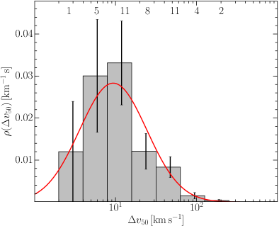
Figure 1: The distribution of 21 cm line widths based on existing detections of intervening absorption at $z>0.1$ (see the text for details of this sample). The sample size in each bin is denoted by the number above and errorbars denote the standard deviation. The solid red line is a log-normal fit to the data, from which we draw random samples for our analysis.

The probability of detecting an absorbing system of given column density depends on the sensitivity of the survey, the flux density and structure of the background source and the fraction of H i in the lower spin state, given by the spin temperature. We express the column density ($N_{\rm HI}$; in atoms cm^-2) in terms of the optical depth ($\tau$) and spin temperature ($T_{\rm spin}$; in K) by

$$N_{\rm HI}=1.823\times 10^{18}\,T_{\rm spin}\int{\tau(v)\mathrm{d}v},$$ (3)

where the integral is performed across the spectral line in the system rest-frame velocity $v$ (in km s^-1). We then express the optical depth in terms of the observables as

$$\tau=-\ln\left[1+{\Delta{S}\over c_{\rm f}S_{\rm cont}}\right],$$ (4)

where $\Delta{S}$ is the observed change in flux density due to absorption, $S_{\rm cont}$ is the background continuum flux density and $c_{\rm f}$ is the (often unknown) fraction of background flux density subtended by the intervening gas.

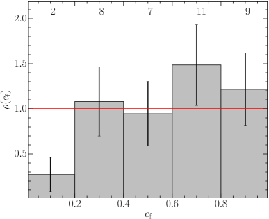
Figure 2: The distribution of H i covering factors from the main sample of Kanekar et al. (2014), which were estimated using the fraction of total continuum flux density in the quasar core. The sample size in each bin is denoted by the number above and errorbars denote the standard deviation. The solid red line is the uniform distribution, from which we draw random samples for our analysis.

We assume that a single intervening system can be described by a Gaussian velocity distribution of full width at half maximum (FWHM) dispersion ($\Delta{v_{\rm 50}}$) and peak optical depth ($\tau_{\rm peak}$), so that Equation 3 can be re-written as

$$N_{\rm HI}=1.941\times 10^{18}\,T_{\rm spin}\,\tau_{\rm peak}\,\Delta{v_{\rm 50}}.$$ (5)

If we further assume that the rms spectral noise is Gaussian, with a standard deviation $\sigma_{\rm chan}$ per independent channel $\Delta{v_{\rm chan}}$, then the 5$\sigma$ column density detection limit is given by

$$N_{5\sigma}\approx 1.941\times 10^{18}\,T_{\rm spin}\,\tau_{\rm 5\sigma}\,\Delta{v_{\rm conv}},$$ (6)

where

$$\tau_{5\sigma}\approx-\ln\left[1-{5\,\sigma_{\rm chan}\over c_{\rm f}\,S_{\rm cont}}\sqrt{\Delta{v}_{\rm chan}\over\Delta{v_{\rm conv}}}\right],$$ (7)

and $\Delta{v_{\rm conv}}\approx\sqrt{\Delta{v}_{\rm chan}^{2}+\Delta{v}_{50}^{2}}$, which is the observed width of the line, given by the convolution of the physical velocity distribution and the spectral resolution of the telescope. We now redefine $\mu$ as the expected number of intervening H i detections in our survey as a function of the column density sensitivity along each sight-line where each comoving path element $\delta{X}(z)$ in the integral defined by Equation 1 is given by

$$\delta{X}(z)=\begin{cases}{\delta{z}\,(1+z)^{2}\over\sqrt{(1+z)^{2}(1+z\Omega_{\rm M})-z(z+2)\Omega_{\rm\Lambda}}},&\text{if}\ N_{\rm HI}\geq N_{5\sigma},\\ 0,&\text{otherwise}.\end{cases}$$ (8)

To calculate the column density sensitivity for each comoving element we draw random samples for $\Delta{v}_{50}$ and $c_{\rm f}$ from continuous prior distributions based on existing evidence. In the case of $\Delta{v}_{50}$ we use a log-normal distribution obtained from a simple least-squares fit to the sample distribution from previous 21-cm absorption surveys reported in the literature (see Figure 1), assuming that this correctly describes the true distribution for the population of DLAs. However, direct measurement of the H i covering factor is significantly more difficult and so for the purposes of this work we draw random samples assuming a uniform distribution between 0 and 1. In Figure 2, we show a comparison between this assumption and the sample distribution estimated by Kanekar et al. (2014) from their main sample of 37 quasars. Kanekar et al. used VLBI synthesis imaging to measure the fraction of total quasar flux density contained within the core, which was then used as a proxy for the covering factor. By carrying out a two-tailed Kolmogorov-Smirnov (KS) test of the hypothesis that the Kanekar et al. data are consistent with our assumed uniform distribution, we find that this hypothesis is rejected at the 0.05 level, but not at the 0.01 level (this outcome is dominated by the paucity of quasars in the sample with $c_{\rm f}\lesssim 0.2$). It is therefore possible that the population distribution of H i covering factors may deviate somewhat from the uniform distribution assumed in this work. We discuss the implications of this further in subsection 5.1.

3 A 21 cm absorption survey with ASKAP

We use the Australian Square Kilometre Array Pathfinder (ASKAP; Johnston et al. 2007) as a case study to demonstrate the expected results from planned wide-field surveys for 21 cm absorption (e.g. the ASKAP First Large Absorption Survey in H i – Sadler et al., the MeerKAT Absorption Line Survey – Gupta et al., and the Search for HI absorption with AperTIF – Morganti et al.). ASKAP is currently undergoing commissioning. Proof-of-concept observations with the Boolardy Engineering Test Array (Hotan et al. 2014) have already been used to successfully detect a new H i absorber associated with a probable young radio galaxy at $z=0.44$ (Allison et al. 2015). Here we predict the outcome of a future 2 h-per-pointing survey of the entire southern sky ($\delta\leq+10\degr$) using the full 36-antenna ASKAP in a single 304 MHz band between 711.5 and 1015.5 MHz, equivalent to H i redshifts between $z=0.4$ and 1.0.

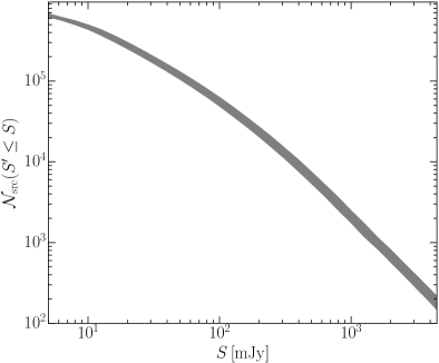
Figure 3: The number of radio sources in our simulated southern sky survey ($\delta\leq+10\degr$) estimated from existing catalogues at $L$-band frequencies (see the text for details). The grey region encloses the expected number across the 711.5 - 1015.5 MHz ASKAP frequency band, assuming a canonical spectral index of $\alpha=-0.7$.

Our expectations of the ASKAP performance are based on preliminary measurements by Chippendale et al. (2015) using the prototype Mark II phase array feed. We estimate the noise per spectral channel using the radiometer equation

$$\sigma_{\rm chan}={S_{\rm system}\over\sqrt{n_{\rm pol}\,n_{\rm ant}\,(n_{\rm ant}-1)\,\Delta{t}_{\rm in}\,\Delta{\nu}_{\rm chan}}},$$ (9)

where $S_{\rm system}$ is the system equivalent flux density, $n_{\rm pol}$ is the number of polarizations, $n_{\rm ant}$ is the number of antennas, $\Delta{t}_{\rm in}$ is the on-source integration time and $\Delta{\nu}_{\rm chan}$ is the spectral resolution in frequency. The sensitivity of the telescope in the 711.5 - 1015.5 MHz band is expected to vary between $S_{\rm system}\approx 3200$ and $2000$ Jy, with the largest change in sensitivity between 700 and 800 MHz. ASKAP has dual linear polarization feeds, 36 antennas and a fine filter bank that produces 16 416 independent channels across the full 304 MHz bandwidth, so the expected noise per 18.5 kHz channel in a 2 h observation is approximately 5.5 - 3.5 mJy beam^-1 across the band. In the case of an actual survey, the true sensitivity will of course be recorded in the spectral data as a function of redshift (see e.g. Allison et al. 2015), but for the purposes of the simulated survey presented in this work we split the band into several frequency bins to capture the variation in sensitivity and velocity resolution (which is in the range 7.8 km s^-1 at 711.5 MHz to 5.5 km s^-1 at 1015.5 MHz).

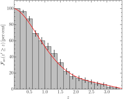
Figure 4: The distribution of CENSORS sources (Brookes et al. 2008) brighter than 10 mJy beyond a given redshift $z$. The red line denotes the cumulative distribution calculated from the parametric model of De Zotti et al. (2010).

In order to simulate a realistic survey of the southern sky we select all radio sources south of $\delta=+10\degr$ from catalogues of the National Radio Astronomy Observatory Very Large Array Sky Survey (NVSS, $\nu=1.4$ GHz, $S_{\rm src}\gtrsim 2.5$ mJy; Condon et al. 1998), the Sydney University Molonglo SkySurvey ($\nu=843$ MHz, $S_{\rm src}\gtrsim 10$ mJy; Mauch et al. 2003) and the second epoch Molonglo Galactic Plane Survey ($\nu=843$ MHz, $S_{\rm src}\gtrsim 10$ mJy; Murphy et al. 2007). The source flux densities, used to calculate the optical depth limit in Equation 7, are estimated at the centre of each frequency bin by extrapolating from the catalogue values and assuming a canonical spectral index of $\alpha=-0.7$. In Figure 3, we show the resulting cumulative distribution of radio sources in our sample as a function of flux density across the band.

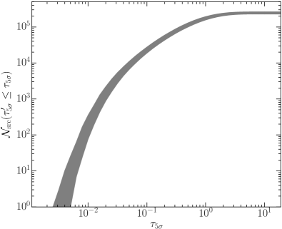
Figure 5: The number of sources in our simulated ASKAP survey with a 21 cm opacity sensitivity greater than or equal to $\tau_{5\sigma}$, as defined by Equation 7. The grey region encloses opacity sensitivities for the 711.5 - 1011.5 MHz band. Random samples for the line FWHM and covering factor were drawn from the distributions shown in Figure 1 and Figure 2.

For any given sight-line, the redshift interval over which absorption may be detected is dependent upon the distance to the continuum source. The lack of accurate spectroscopic redshift measurements for most radio sources over the sky necessitates the use of a statistical approach based on a model for the source redshift distribution. We therefore apply a statistical weighting to each comoving path element $\delta{X}(z)$ such that the expected number of absorber detections is now given by

$$\mu=\iint{f(N_{\rm HI},X)\,\mathcal{F}_{\rm src}(z^{\prime}\geq z)\,\mathrm{d}X\,\mathrm{d}N_{\rm HI}},$$ (10)

where

$$\mathcal{F}_{\rm src}(z^{\prime}\geq z)={\int_{z}^{\infty}\mathcal{N}_{\rm src}(z^{\prime})\mathrm{d}z^{\prime}\over\int_{0}^{\infty}\mathcal{N}_{\rm src}(z^{\prime})\mathrm{d}z^{\prime}},$$ (11)

and $\mathcal{N}_{\rm src}(z)$ is the number of radio sources as a function of redshift. To estimate $\mathcal{N}_{\rm src}(z)$ we use the Combined EIS-NVSS Survey Of Radio Sources (CENSORS; Brookes et al. 2008), which forms a complete sample of radio sources brighter than 7.2 mJy at 1.4 GHz with spectroscopic redshifts out to cosmological distances. In Figure 4 we show the distribution of CENSORS sources brighter than 10 mJy beyond a given redshift $z$, and the corresponding analytical function derived from the model fit of De Zotti et al. (2010), given by

$$\mathcal{N}_{\rm src}(z)\approx 1.29+32.37z-32.89z^{2}+11.13z^{3}-1.25z^{4},$$ (12)

which we use in our analysis. For the redshifts spanned by our simulated ASKAP survey, the fraction of background sources evolves from 87 per cent at $z=0.4$ to 53 per cent at $z=1.0$.

We assume that this redshift distribution applies to any sight-line irrespective of the continuum flux density. However, this assumption is only true if the source population in the target sample evolves such that the effect of distance is nullified by an increase in luminosity. Given this criterion, and the sensitivity of our simulated survey, we limit our sample to sources with flux densities between 10 and 1000 mJy, which are dominated by the rapidly evolving population of high-excitation radio galaxies and quasars (e.g. Jackson & Wall 1999; Best & Heckman 2012; Best et al. 2014; Pracy et al. 2016) and for which the redshift distribution is known to be almost independent of flux density (e.g. Condon 1984; Condon et al. 1998). In Figure 5, we show the number of sources from this sub-sample as a function of opacity sensitivity [as defined by Equation 7], drawing random samples of the line FWHM and covering factor from the distributions shown in Figure 1 and Figure 2. There are approximately 190 000 sightlines with sufficient sensitivity to detect absorption of optical depth greater than $\tau_{5\sigma}\approx 1.0$ and 25 000 sensitive to optical depths greater than $\tau_{5\sigma}\approx 0.1$. Since this distribution converges at optical depth sensitivities greater than $\tau_{5\sigma}\approx 5$, the population of sources fainter than 10 mJy, which are excluded from our simulated ASKAP survey, would not significantly contribute to further detections of absorption. Similarly, while sources brighter than 1 Jy are good probes of low-column-density H i gas, they do not constitute a sufficiently large enough population to significantly affect the total number of absorber detections expected in the survey and can also be safely excluded.

Based on these assumptions, we can estimate the number of absorbers we would expect to detect in our survey with ASKAP as a function of spin temperature. In Figure 6, we show the expected detection yield as a cumulative function of column density. We show results for two scenarios where the spin temperature is fixed at a single value of either 100 or 1000 K, and the line FWHM and covering factors are drawn from the random distributions shown in Figure 1 and Figure 2. We find that for both these cases the expected number of detections is not sensitive to column densities below the DLA definition of $N_{\rm HI}=2\times 10^{20}$ cm^-2. We also show in Figure 7 the expected total detection yield (integrated over all H i column densities) as a function of a single spin temperature $T_{\mathrm{spin}}$ and line FWHM $\Delta{v}_{\mathrm{50}}$. We find that for typical spin temperatures of a few hundred kelvin (consistent with the typical fraction of CNM observed in the local Universe) and a line FWHM of approximately $20$ km s^-1, a wide-field 21 cm survey with ASKAP is expected to yield $\sim 1000$ detections. However, even moderate evolution to a higher spin temperature in the DLA population should see significant reduction in the detection yield from this survey.

4 Inferring the average spin temperature

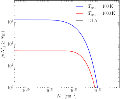
Figure 6: The expected number of absorber detections (as a cumulative function of column density) in our simulated ASKAP survey. We show two scenarios for a single spin temperature $T_{\rm spin}=100$ and $1000$ K, where we have drawn random samples for the line FWHM and covering factor from the distributions shown in Figure 1 and Figure 2. In both cases we find that the expected number of detections is not sensitive to column densities below $N_{\rm HI}=2\times 10^{20}$ cm^-2, indicating that such a survey will only be sensitive to DLA systems.

We cannot directly measure the spin temperatures of individual systems without additional data from either 21 cm emission or Lyman-$\alpha$ absorption. However, from Figure 7 it is evident that the total number of absorbing systems expected to be detected with a reasonably large 21 cm survey is strongly dependent on the assumed value for the spin temperature. Therefore, by comparing the actual survey yield with that expected from the known H i distribution, we can infer the average spin temperature of the atomic gas within the DLA population for a given redshift interval.

Assuming that the total number of detections follows a Poisson distribution, the probability of detecting $\mathcal{N}$ intervening absorbing systems is given by

$$p(\mathcal{N}|\overline{\mu})={\overline{\mu}^{\mathcal{N}}\over\mathcal{N}!}\mathrm{e}^{-\overline{\mu}},$$ (13)

where $\overline{\mu}$ is the expected total number of detections given by the integral

$$\overline{\mu}=\iiint{\mu(T_{\rm spin},\Delta{v}_{50},c_{\rm f})\rho(T_{\rm spin},\Delta{v}_{50},c_{\rm f})\mathrm{d}T_{\rm spin}\mathrm{d}\Delta{v}_{50}\mathrm{d}c_{\rm f}},$$ (14)

and $\rho$ is the distribution of systems as a function of spin temperature, line FWHM and covering factor. We assume that all three of these variables are independent so that $\rho$ factorizes into functions of each. We then marginalise over the covering factor and line width distributions shown in Figure 1 and Figure 2 so that the expression for $\overline{\mu}$ reduces to

$$\overline{\mu}=\int{\mu(T_{\rm spin})\rho(T_{\rm spin})\mathrm{d}T_{\rm spin}}=\mu(\overline{T}_{\rm spin}),$$ (15)

where $\overline{T}_{\rm spin}$ is the harmonic mean of the unknown spin temperature distribution, weighted by column density. This is analogous to the spin temperature inferred from the detection of absorption in a single intervening galaxy averaged over several gaseous components at different temperatures (e.g. Carilli et al. 1996).

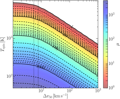
Figure 7: The expected total number of detections in our simulated ASKAP survey, as a function of a single spin temperature ($T_{\rm spin}$) and line FWHM ($\Delta{v}_{50}$). The vertical dotted lines enclose the velocity resolution across the observed frequency band. We draw random samples for the covering factor from a uniform distribution between 0 and 1 (as shown in Figure 2). The contours are truncated at $\mu<1$ for clarity.

In the event of the survey yielding $\mathcal{N}$ detections, we can calculate the posterior probability density of $\overline{T}_{\rm spin}$ using the following relationship between conditional probabilities

$$p(\overline{T}_{\rm spin}|\mathcal{N})={p(\mathcal{N}|\overline{T}_{\rm spin})p(\overline{T}_{\rm spin})\over p(\mathcal{N})},$$ (16)

where $p(\overline{T}_{\rm spin})$ is our prior probability density for $\overline{T}_{\rm spin}$ and $p(\mathcal{N})$ is the marginal probability of the number of detections, which can be treated as a normalizing constant. The minimally informative Jeffreys prior for the mean value $\mu$ of a Poisson distribution is $1/\sqrt{\mu}$ (Jeffreys 1946). From Equation 15 it therefore follows that a suitable form for the non-informative spin temperature prior is $p(\overline{T}_{\rm spin})=1/\sqrt{\overline{\mu}}$, so that

$$p(\overline{T}_{\rm spin}|\mathcal{N})=C^{-1}\,{\overline{\mu}^{(\mathcal{N}-1/2)}\over\mathcal{N}!}\mathrm{e}^{-\overline{\mu}},$$ (17)

where the distribution is normalised to unit total probability by evaluating the integral

$$C=\int{{\overline{\mu}^{(\mathcal{N}-1/2)}\over\mathcal{N}!}\mathrm{e}^{-\overline{\mu}}}\,\mathrm{d}\overline{T}_{\rm spin}.$$ (18)

The probabilistic relationship given by Equation 17 and the expected detection yield derived in section 3 can be used as a frame-work for inferring the harmonic-mean spin temperature using the results of any homogeneous 21-cm survey. We have assumed that we can accurately distinguish intervening absorbing systems from those associated with the host galaxy of the radio source. However, any 21-cm survey will be accompanied by follow-up observations, at optical and sub-mm wavelengths, which will aid identification. Furthermore, future implementation of probabilistic techniques to either use photometric redshift information or distinguish between line profiles should provide further disambiguation.

Of course we have not yet accounted for any error in our estimate of $\overline{\mu}$, which will increase our uncertainty in $\overline{T}_{\mathrm{spin}}$. In the following section we discuss these possible sources of error and their effect on the result.

5 Sources of error

Our estimate of the expected number of 21 cm absorbers is dependent upon several distributions describing the properties of the foreground absorbing gas and the background source distribution. For future large-scale 21 cm surveys, the accuracy to which we can infer the harmonic mean of the spin temperature distribution will eventually be limited by the accuracy to which we can measure these other distributions. In this section, we describe these errors and their propagation through to the estimate of $\overline{T}_{\mathrm{spin}}$, summarizing our results in Table 1.

5.1 The covering factor

5.1.1 Deviation from a uniform distribution between 0 and 1

The fraction $c_{\rm f}$ by which the foreground gas subtends the background radiation source is difficult to measure directly and is thereby a significant source of error for 21 cm absorption surveys. In this work, we have assumed a uniform distribution for $c_{\rm f}$, taking random values between 0 and 1. In section 2, we tested this assumption by comparing it with the distribution of flux density core fractions in a sample of 37 quasars, used by Kanekar et al. (2014) as a proxy for the covering factor. By carrying out a two-tailed KS test, we found some evidence (at the 0.05 level) that this quasar sample was inconsistent with our assumption of a uniform distribution between 0 and 1. Noticeably there seems to be an under-representation of quasars in the Kanekar et al. sample with estimated $c_{\rm f}\lesssim 0.2$. In the low optical depth limit, the detection rate is dependent on the ratio of spin temperature to covering factor, in which case a fractional deviation in $c_{\rm f}$ will propagate as an equal fractional deviation in $\overline{T}_{\mathrm{spin}}$. Based on the difference seen in the covering factor distribution of the Kanekar et al. sample and the uniform distribution, we assume that the spin temperature can deviate by as much as $\pm$10 per cent.

5.1.2 Evolution with redshift

We also consider that the covering factor distribution may evolve with redshift, which would mimic a perceived evolution in the average spin temperature. Such an effect was proposed by Curran & Webb (2006) and Curran (2012), who claimed that the relative change in angular-scale behaviour of absorbers and radio sources between low- and high-redshift samples could explain the apparent evolution of the spin temperature found by Kanekar & Chengalur (2003). To test for this effect in their larger DLA sample, Kanekar et al. (2014) considered a sub-sample at redshifts greater than $z=1$, for which the relative evolution of the absorber and source angular sizes should be minimal. While the significance of their result was reduced by removing the lower redshift absorbers from their sample, they still found a difference at $3.5\,\sigma$ significance between spin temperature distributions in the two DLA sub-samples separated by a median redshift of $z=2.683$.

Future surveys with ASKAP and the other SKA pathfinders will search for H i absorption at intermediate redshifts ($z\sim 1$), where the relative evolution of the absorber and source angular sizes is expected to be more significant than for the higher redshift DLA sample considered by Kanekar et al. (2014). We therefore consider the potential effect of this cosmological evolution on the inferred value of $\overline{T}_{\mathrm{spin}}$. We approximate the covering factor using the following model of Curran & Webb (2006)

$$c_{f}\approx\begin{cases}\left({\theta_{\rm abs}\over\theta_{\rm src}}\right)^{2},&\text{if}\ \theta_{\rm abs}<\theta_{\rm src},\\ 1,&\text{otherwise},\end{cases}$$ (19)

where $\theta_{\rm abs}$ and $\theta_{\rm src}$ are the angular sizes of the absorber and background source, respectively. Under the small-angle approximation $\theta_{\rm abs}\approx{d_{\rm abs}/D_{\rm abs}}$ and $\theta_{\rm abs}\approx{d_{\rm src}/D_{\rm src}}$, where $d_{\rm abs}$ and $D_{\rm abs}$ are the linear size and angular diameter distance of the absorber, and likewise $d_{\rm src}$ and $D_{\rm src}$ are the linear size and angular diameter distance of the background source. Assuming that the ratio $d_{\rm abs}/d_{\rm src}$ is randomly distributed and independent of redshift, any evolution in the covering factor is therefore dominated by relative changes in the angular diameter distances. We calculate the expected angular diameter distance ratio at a redshift $z$ by

$$\left\langle{D_{\rm abs}\over D_{\rm src}}\right\rangle_{z}=D_{\rm abs}(z){\int_{z}^{\infty}\mathcal{N}_{\rm src}(z^{\prime})D_{\rm src}(z^{\prime})^{-1}\mathrm{d}z^{\prime}\over\int_{z}^{\infty}\mathcal{N}_{\rm src}(z^{\prime})\mathrm{d}z^{\prime}},$$ (20)

which, for the source redshift distribution model given by De Zotti et al. (2010), evolves from 0.7 at $z=0.4$ to 1.0 at $z=1.0$ (see Figure 8). We note that this is consistent with the behaviour measured by Curran (2012) for the total sample of DLAs observed at 21 cm wavelengths. By applying this as a correction to the otherwise uniformly distributed covering factor (using Equation 19), we find that the inferred value of $\overline{T}_{\rm spin}$ systematically increases by approximately 30 per cent.

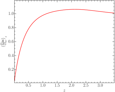
Figure 8: The expected redshift behaviour of $D_{\rm abs}/D_{\rm src}$ based on the De Zotti et al. (2010) model for the radio source redshift distribution.

5.2 The $\mn@boldsymbol{N_{\rm HI}}$ frequency distribution

5.2.1 Uncertainty in the measurement of $f(N_{\rm HI},X)$

We assume that $f(N_{\rm HI},X)$ is relatively well understood as a function of redshift by interpolating between model gamma functions fitted to the distributions at $z=0$ and $3$. However, these distributions were measured from finite samples of galaxies, which of course have associated uncertainties that need to be considered. In the case of the data presented by Zwaan et al. (2005) and Noterdaeme et al. (2009), both have typical measurement uncertainties in $f(N_{\rm HI},X)$ of approximately 10 per cent over the range of column densities for which our simulated ASKAP survey is sensitive (see Figure 6). This will propagate as a 10 per cent fractional error in the expected number of absorber detections, and contribute a similar percentage uncertainty in the inferred average spin temperature.

5.2.2 Correcting for 21 cm self-absorption

In the local Universe, Braun (2012) showed that self-absorption from opaque H i clouds identified in high-resolution images of the Local Group galaxies M31, M33 and the Large Magellanic Cloud may necessitate a correction to the local atomic mass density of up to 30 per cent. Although it is not yet clear whether this small sample of Local Group galaxies is representative of the low-redshift population, it is useful to understand how this effect might propagate through to our average spin temperature measurement. We therefore replace the gamma-function parametrization of the local $f(N_{\rm HI})$ given by Zwaan et al. (2005) with the non-parametric values given in table 2 of Braun (2012), and recalculate $\overline{T}_{\rm spin}$. For an all-sky survey with the full 36-antenna ASKAP we find that $\overline{T}_{\rm spin}$ increases by $\sim$30 for 100 detections and $\sim$10 per cent for 1000 detections. Note that the correction increases for low numbers of detections, which are dominated by the highest column density systems.

5.2.3 Dust obscuration bias in optically-selected DLAs

At higher redshifts, it is possible that the number density of optically-selected DLAs could be significantly underestimated as a result of dust obscuration of the background quasar (Ostriker & Heisler 1984). This would cause a reduction in the $f(\mbox{H\,{\sc i}},X)$ measured from optical surveys, thereby significantly underestimating the expected number of intervening 21 cm absorbers at high redshifts. The issue is further compounded by the expectation that the highest column density DLAs ($N_{\rm HI}\gtrsim 10^{21}$ cm^-2), for which future wide-field 21 cm surveys are most sensitive (see Figure 6), may contain more dust than their less-dense counterparts.

This conclusion was supported by early analyses of the existing quasar surveys at that time (e.g. Fall & Pei 1993), which indicated that up to 70 per cent of quasars could be missing from optical surveys through the effect of dust obscuration, albeit with large uncertainties. However, subsequent optical and infrared observations of radio-selected quasars (e.g. Ellison et al. 2001; Ellison, Hall & Lira 2005; Jorgenson et al. 2006), which are free of the potential selection biases associated with these optical surveys, found that the severity of this issue was substantially over-estimated and that there was minimal evidence in support of a correlation between the presence of DLAs and dust reddening. Furthermore, the H i column density frequency distribution measured by Jorgenson et al. (2006) was found to be consistent with the optically-determined gamma-function parametrization of Prochaska et al. (2005), with no evidence of DLA systems missing from the SDSS sample at a sensitivity of $N_{\rm HI}\lesssim 5\times 10^{21}$ cm^-2. Although radio-selected surveys of quasars are free of the selection biases associated with optical surveys, they do typically suffer from smaller sample sizes and are therefore less sensitive to the rarer DLAs with the highest column densities.

Another approach is to directly test whether optically-selected quasars with intervening DLAs, selected from the SDSS sample, are systematically more dust reddened than a control sample of non-DLA quasars. Comparisons in the literature are based on several different colour indicators, which include the spectral index (e.g. Murphy & Liske 2004; Murphy & Bernet 2016), spectral stacking (e.g. Frank & Péroux 2010; Khare et al. 2012) and direct photometry (e.g. Vladilo, Prochaska & Wolfe 2008; Fukugita & Ménard 2015). The current status of these efforts is summarized by Murphy & Bernet (2016), showing broad support for a missing DLA population at the level of $\sim$5 per cent but highlighting that tension still exists between different dust measurements. No substantial evidence has yet been found to support a correlation between the dust reddening and H i column density in these optically selected DLA surveys (e.g. Vladilo et al. 2008; Khare et al. 2012; Murphy & Bernet 2016).

In an attempt to reconcile the differences and myriad biases associated with these techniques, Pontzen & Pettini (2009) carried out a statistically-robust meta-analysis of the available optical and radio data, using a Bayesian parameter estimation approach to model the dust as a function of column density and metallicity. They found that the expected fraction of DLAs missing from optical surveys is 7 per cent, with fewer than 28 per cent missing at 3 $\sigma$ confidence. Based on this body of work we therefore assume that approximately 10 per cent of DLAs are missing from the SDSS sample of Noterdaeme et al. (2009) and consider the affect on our estimate of $\overline{T}_{\rm spin}$. We further assume that there is no dependance on column density, an assumption which is supported by the aforementioned observational data for the range of column densities to which our 21 cm survey is sensitive. We find that increasing the high-redshift column density frequency distribution by 10 per cent introduces a systematic increase of approximately 3 per cent in the expected number of detections for the redshifts covered by our ASKAP surveys. We note that this error will increase significantly for 21 cm surveys at higher redshifts where the optically derived $f(\mbox{H\,{\sc i}},X)$ dominates the calculation of the expected detection rate.

5.3 The radio source background

As described in section 3, we weight the comoving path-length for each sight-line by a statistical redshift distribution in order to account for evolution in the radio source background. We use the parametric model of De Zotti et al. (2010), which is derived from fitting the measured redshifts of Brookes et al. (2008) for CENSORS sources brighter than 10 mJy, and assume that this applies to all sources in the range 10 - 1000 mJy. In Figure 4, we show the cumulative distribution of sources located behind a given redshift and the associated measurement uncertainty given by the errorbars. For the intermediate redshifts covered by the ASKAP survey, the fractional uncertainty in this distribution increases from $\sigma_{\mathcal{F}_{\rm src}}/\mathcal{F}_{\rm src}\approx 3.5$ to 8 per cent between $z=0.4$ and 1.0, which propagates through to a similar fractional uncertainty in $\overline{T}_{\rm spin}$. However, for higher redshifts this fractional uncertainty increases rapidly at $z>2$, to more than 50 per cent at $z=3$, reflecting the paucity of optical spectroscopic data for the high-redshift radio source population. Understanding how the radio source population is distributed at lower flux densities and at higher redshifts is therefore a concern for the future 21 cm absorption surveys undertaken with the SKA mid- and low-frequency telescopes (see Kanekar & Briggs 2004 and Morganti, Sadler & Curran 2015 for reviews).

Table 1: An account of errors in our estimate of $\overline{T}_{\rm spin}$ due to the accuracy to which we can determine the expected number of absorber detections.

	Source of error	$\mathrm{err}(\overline{T}_{\rm spin})$	Refs.
		[per cent]
Covering factor	Distribution uncertainty	$\pm 10$	$a$
Covering factor	Systematic evolution	+30	$a$, $b$
$f(N_{\rm HI},X)$	Measurement uncertainty	$\pm 10$	$c,d$
Low-$z$ $f(N_{\rm HI},X)$	Systematic self-absorption	$+(10-30)$	$e$
High-$z$ $f(N_{\rm HI},X)$	Systematic dust-obscuration	$+3$	$f$, $g$
$\mathcal{F}_{\rm src}(z^{\prime}\geq z)$	Measurement uncertainty	$\pm 5$	$h$, $i$

• References: ^aKanekar et al. (2014), ^bCurran (2012), ^cZwaan et al. (2005), ^dNoterdaeme et al. (2009) , ^eBraun (2012), ^fPontzen & Pettini (2009), ^gMurphy & Bernet (2016), ^hBrookes et al. (2008), ⁱDe Zotti et al. (2010).

6 Expected results for future 21-cm absorption surveys

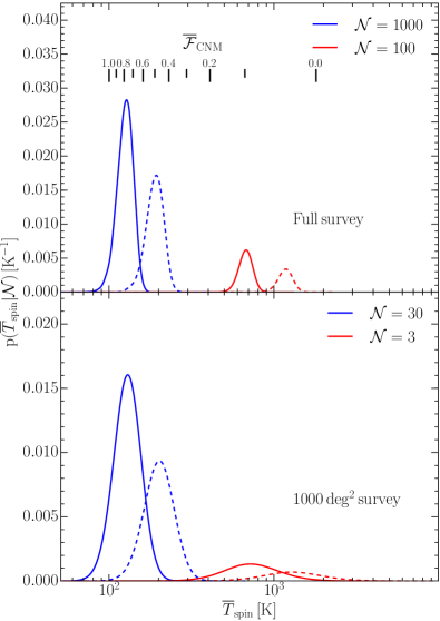
Figure 9: The posterior probability density of the average spin temperature, as a function of absorber detection yield ($\mathcal{N}$). We show results for our simulated all-southern-sky survey with 2-h per pointing using the full 36-antenna ASKAP (top panel) and a smaller 1000 deg² survey with 12-h per pointing and 12 antennas of ASKAP (bottom panel). The dashed curves show the cumulative effect of the systematic errors discussed in section 5. $\overline{\mathcal{F}}_{\rm CNM}$ is the average CNM fraction assuming a simple two-phase neutral ISM with $T_{\rm spin,CNM}=100$ K and $T_{\rm spin,WNM}=1800$ K (Liszt 2001).

In the top panel of Figure 9 we show the results of applying our method for inferring $\overline{T}_{\rm spin}$ to the simulated all-southern-sky H i absorption survey with ASKAP described in section 3. We account for the uncertainties in the expected detection rate $\overline{\mu}$, discussed in section 5, by using a Monte Carlo approach and marginalizing over many realizations. A yield of 1000 absorbers from such a survey would imply an average spin temperature of $\overline{T}_{\mathrm{spin}}=127^{+14}_{-14}\,(193^{+23}_{-23})$ K, where values in parentheses denote the alternative posterior probability resulting from the systematic errors discussed in section 5. This scenario would indicate that a large fraction of the atomic gas in DLAs at these intermediate redshifts is in the classical stable CNM phase. Conversely, a yield of only 100 detections would imply that $\overline{T}_{\mathrm{spin}}=679^{+64}_{-65}\,(1184^{+116}_{-120})$ K, indicating that less than 10 per cent of the atomic gas is in the CNM and that the bulk of the neutral gas in galaxies is significantly different at intermediate redshifts compared with the local Universe.

We also consider the effect of reducing the sky area and array size, which is relevant for planned early science surveys with ASKAP and other SKA pathfinder telescopes. In the bottom panel of Figure 9, we show the spin temperatures inferred when observing a random 1000 deg² field for 12 h per pointing, between $z_{\rm HI}=0.4$ and $1.0$, using a 12-antenna version of ASKAP. We find that detection yields of 30 and 3 from such a survey would give inferred spin temperatures of $\overline{T}_{\rm spin}=134^{+23}_{-27}\,(209^{+40}_{-47})$ and $848^{+270}_{-430}\,(1535^{+513}_{-837})$ K, respectively. The significant reduction in telescope sensitivity and sky-area, compensated by the increase in integration time per pointing planned for early-science, results in a factor of 30 decrease in the expected number of detections and therefore an increase in the sample variance and uncertainty in $\overline{T}_{\rm spin}$. However, this result demonstrates that we expect to be able to distinguish between the limiting cases of CNM-rich or deficient DLA populations even during the early-science phases of the SKA pathfinders. For example 30 detections with the early ASKAP survey rules out an average spin temperature of 1000 K at high probability.

7 Conclusions

We have demonstrated a statistical method for measuring the average spin temperature of the neutral ISM in distant galaxies, using the expected detection yields from future wide-field 21 cm absorption surveys. The spin temperature is a crucial property of the ISM that can be used to determine the fraction of the cold ($T_{\rm k}\sim 100$ K) and dense ($n\sim 100$ cm^-2) atomic gas that provides sites for the future formation of cold molecular gas clouds and star formation. Recent 21 cm surveys for H i absorption in Mg ii absorbers and DLAs towards distant quasars have yielded some evidence of an evolution in the average spin temperature that might reveal a decrease in the fraction of cold dense atomic gas at high redshift (e.g. Gupta et al. 2009; Kanekar et al. 2014).

By combining recent specifications for ASKAP, with available information for the population of background radio sources, we show that strong statistical constraints (approximately $\pm 10$ per cent) in the average spin temperature can be achieved by carrying out a shallow 2-h per pointing survey of the southern sky between redshifts of $z=0.4$ and $1.0$. However, we find that the accuracy to which we can measure the average spin temperature is ultimately limited by the accuracy to which we can measure the distribution of the covering factor, the $N_{\rm HI}$ frequency distribution function and the evolution of the radio source population as a function of redshift. By improving our understanding of these distributions we will be able to leverage the order-of-magnitude increases in sensitivity and redshift coverage of the future SKA telescope, allowing us to measure the evolution of the average spin temperature to much higher redshifts.

References

- Allison et al. (2015) Allison J. R., et al., 2015, MNRAS, 453, 1249
- Astropy Collaboration et al. (2013) Astropy Collaboration et al., 2013, A&A, 558, A33
- Bahcall & Ekers (1969) Bahcall J. N., Ekers R. D., 1969, ApJ, 157, 1055
- Best & Heckman (2012) Best P. N., Heckman T. M., 2012, MNRAS, 421, 1569
- Best et al. (2014) Best P. N., Ker L. M., Simpson C., Rigby E. E., Sabater J., 2014, MNRAS, 445, 955
- Braun (2012) Braun R., 2012, ApJ, 749, 87
- Braun et al. (2009) Braun R., Thilker D. A., Walterbos R. A. M., Corbelli E., 2009, ApJ, 695, 937
- Briggs et al. (2001) Briggs F. H., de Bruyn A. G., Vermeulen R. C., 2001, A&A, 373, 113
- Brookes et al. (2008) Brookes M. H., Best P. N., Peacock J. A., Röttgering H. J. A., Dunlop J. S., 2008, MNRAS, 385, 1297
- Brüns et al. (2005) Brüns C., et al., 2005, A&A, 432, 45
- Carilli et al. (1993) Carilli C. L., Rupen M. P., Yanny B., 1993, ApJL, 412, L59
- Carilli et al. (1996) Carilli C. L., Lane W., de Bruyn A. G., Braun R., Miley G. K., 1996, AJ, 111, 1830
- Carswell et al. (2011) Carswell R. F., Jorgenson R. A., Wolfe A. M., Murphy M. T., 2011, MNRAS, 411, 2319
- Carswell et al. (2012) Carswell R. F., Becker G. D., Jorgenson R. A., Murphy M. T., Wolfe A. M., 2012, MNRAS, 422, 1700
- Chengalur & Kanekar (2000) Chengalur J. N., Kanekar N., 2000, MNRAS, 318, 303
- Chengalur et al. (1999) Chengalur J. N., de Bruyn A. G., Narasimha D., 1999, A&A, 343, L79
- Chippendale et al. (2015) Chippendale A. P., et al., 2015, in 2015 International Conference on Electromagnetics in Advanced Applications (ICEAA). IEEE, pp 541 – 544 (arXiv:1509.00544)
- Condon (1984) Condon J. J., 1984, ApJ, 287, 461
- Condon et al. (1998) Condon J. J., Cotton W. D., Greisen E. W., Yin Q. F., Perley R. A., Taylor G. B., Broderick J. J., 1998, AJ, 115, 1693
- Cooke et al. (2015) Cooke R. J., Pettini M., Jorgenson R. A., 2015, ApJ, 800, 12
- Curran (2012) Curran S. J., 2012, ApJ, 748, L18
- Curran & Webb (2006) Curran S. J., Webb J. K., 2006, MNRAS, 371, 356
- Curran et al. (2005) Curran S. J., Murphy M. T., Pihlström Y. M., Webb J. K., Purcell C. R., 2005, MNRAS, 356, 1509
- Curran et al. (2007) Curran S. J., Darling J., Bolatto A. D., Whiting M. T., Bignell C., Webb J. K., 2007, MNRAS, 382, L11
- Darling et al. (2011) Darling J., Macdonald E. P., Haynes M. P., Giovanelli R., 2011, ApJ, 742, 60
- Davis & May (1978) Davis M. M., May L. S., 1978, ApJ, 219, 1
- De Zotti et al. (2010) De Zotti G., Massardi M., Negrello M., Wall J., 2010, A&AR, 18, 1
- Ellison et al. (2001) Ellison S. L., Yan L., Hook I. M., Pettini M., Wall J. V., Shaver P., 2001, A&A, 379, 393
- Ellison et al. (2005) Ellison S. L., Hall P. B., Lira P., 2005, AJ, 130, 1345
- Ellison et al. (2012) Ellison S. L., Kanekar N., Prochaska J. X., Momjian E., Worseck G., 2012, MNRAS, 424, 293
- Fall & Pei (1993) Fall S. M., Pei Y. C., 1993, ApJ, 402, 479
- Fernández et al. (2016) Fernández X., et al., 2016, ApJL, 824, L1
- Field (1958) Field G. B., 1958, Proc. IRE, 46, 240
- Field (1959) Field G. B., 1959, ApJ, 129, 536
- Field et al. (1969) Field G. B., Goldsmith D. W., Habing H. J., 1969, ApJL, 155, L149
- Frank & Péroux (2010) Frank S., Péroux C., 2010, MNRAS, 406, 2235
- Fukugita & Ménard (2015) Fukugita M., Ménard B., 2015, ApJ, 799, 195
- Giovanelli & Haynes (2016) Giovanelli R., Haynes M. P., 2016, A&AR, 24, 1
- Gratier et al. (2010) Gratier P., et al., 2010, A&A, 522, A3
- Gupta et al. (2009) Gupta N., Srianand R., Petitjean P., Noterdaeme P., Saikia D. J., 2009, MNRAS, 398, 201
- Gupta et al. (2012) Gupta N., Srianand R., Petitjean P., Bergeron J., Noterdaeme P., Muzahid S., 2012, A&A, 544, A21
- Gupta et al. (2013) Gupta N., Srianand R., Noterdaeme P., Petitjean P., Muzahid S., 2013, A&A, 558, A84
- Haynes et al. (2011) Haynes M. P., et al., 2011, AJ, 142, 170
- Heiles & Troland (2003) Heiles C., Troland T. H., 2003, ApJ, 586, 1067
- Hotan et al. (2014) Hotan A. W., et al., 2014, Publ. Astron. Soc. Aust., 31, e041
- Howk et al. (2005) Howk J. C., Wolfe A. M., Prochaska J. X., 2005, ApJL, 622, L81
- Jackson & Wall (1999) Jackson C. A., Wall J. V., 1999, MNRAS, 304, 160
- Jeffreys (1946) Jeffreys H., 1946, Proc. R. Soc. A, 186
- Jeffreys (1961) Jeffreys H., 1961, Theory of Probability, third edn. Clarendon Press, Oxford
- Johnston et al. (2007) Johnston S., et al., 2007, Publ. Astron. Soc. Aust., 24, 174
- Jorgenson et al. (2006) Jorgenson R. A., Wolfe A. M., Prochaska J. X., Lu L., Howk J. C., Cooke J., Gawiser E., Gelino D. M., 2006, ApJ, 646, 730
- Jorgenson et al. (2010) Jorgenson R. A., Wolfe A. M., Prochaska J. X., 2010, ApJ, 722, 460
- Kanekar (2014) Kanekar N., 2014, ApJL, 797, L20
- Kanekar & Briggs (2003) Kanekar N., Briggs F. H., 2003, A&A, 412, L29
- Kanekar & Briggs (2004) Kanekar N., Briggs F. H., 2004, New Astron. Rev., 48, 1259
- Kanekar & Chengalur (2001) Kanekar N., Chengalur J. N., 2001, A&A, 369, 42
- Kanekar & Chengalur (2003) Kanekar N., Chengalur J. N., 2003, A&A, 399, 857
- Kanekar et al. (2001) Kanekar N., Ghosh T., Chengalur J. N., 2001, A&A, 373, 394
- Kanekar et al. (2006) Kanekar N., Subrahmanyan R., Ellison S. L., Lane W. M., Chengalur J. N., 2006, MNRAS, 370, L46
- Kanekar et al. (2007) Kanekar N., Chengalur J. N., Lane W. M., 2007, MNRAS, 375, 1528
- Kanekar et al. (2009) Kanekar N., Prochaska J. X., Ellison S. L., Chengalur J. N., 2009, MNRAS, 396, 385
- Kanekar et al. (2013) Kanekar N., Ellison S. L., Momjian E., York B. A., Pettini M., 2013, MNRAS, 428, 532
- Kanekar et al. (2014) Kanekar N., et al., 2014, MNRAS, 438, 2131
- Khare et al. (2012) Khare P., vanden Berk D., York D. G., Lundgren B., Kulkarni V. P., 2012, MNRAS, 419, 1028
- Kim et al. (2003) Kim S., Staveley-Smith L., Dopita M. A., Sault R. J., Freeman K. C., Lee Y., Chu Y.-H., 2003, ApJS, 148, 473
- Lagos et al. (2014) Lagos C. D. P., Baugh C. M., Zwaan M. A., Lacey C. G., Gonzalez-Perez V., Power C., Swinbank A. M., van Kampen E., 2014, MNRAS, 440, 920
- Lane & Briggs (2001) Lane W. M., Briggs F. H., 2001, ApJL, 561, L27
- Lane et al. (2000) Lane W. M., Briggs F. H., Smette A., 2000, ApJ, 532, 146
- Lehner et al. (2008) Lehner N., Howk J. C., Prochaska J. X., Wolfe A. M., 2008, MNRAS, 390, 2
- Liszt (2001) Liszt H., 2001, A&A, 371, 698
- Lovell et al. (1996) Lovell J. E. J., et al., 1996, ApJ, 472, L5
- Mauch et al. (2003) Mauch T., Murphy T., Buttery H. J., Curran J., Hunstead R. W., Piestrzynski B., Robertson J. G., Sadler E. M., 2003, MNRAS, 342, 1117
- McClure-Griffiths et al. (2009) McClure-Griffiths N. M., et al., 2009, ApJS, 181, 398
- McKee & Ostriker (1977) McKee C. F., Ostriker J. P., 1977, ApJ, 218, 148
- Morganti et al. (2015) Morganti R., Sadler E. M., Curran S., 2015, in Advancing Astrophysics with the Square Kilometre Array (AASKA14). p. 134 (arXiv:1501.01091)
- Murphy & Bernet (2016) Murphy M. T., Bernet M. L., 2016, MNRAS, 455, 1043
- Murphy & Liske (2004) Murphy M. T., Liske J., 2004, MNRAS, 354, L31
- Murphy et al. (2007) Murphy T., Mauch T., Green A., Hunstead R. W., Piestrzynska B., Kels A. P., Sztajer P., 2007, MNRAS, 382, 382
- Murray et al. (2015) Murray C. E., et al., 2015, ApJ, 804, 89
- Neeleman et al. (2015) Neeleman M., Prochaska J. X., Wolfe A. M., 2015, ApJ, 800, 7
- Neeleman et al. (2016) Neeleman M., Prochaska J. X., Ribaudo J., Lehner N., Howk J. C., Rafelski M., Kanekar N., 2016, ApJ, 818, 113
- Noterdaeme et al. (2009) Noterdaeme P., Petitjean P., Ledoux C., Srianand R., 2009, A&A, 505, 1087
- Novick & Hall (1965) Novick M. R., Hall W. J., 1965, J. Am. Stat. Assoc., 60, 1104
- Ostriker & Heisler (1984) Ostriker J. P., Heisler J., 1984, ApJ, 278, 1
- Pontzen & Pettini (2009) Pontzen A., Pettini M., 2009, MNRAS, 393, 557
- Pracy et al. (2016) Pracy M. B., et al., 2016, MNRAS, 460, 2
- Prochaska et al. (2005) Prochaska J. X., Herbert-Fort S., Wolfe A. M., 2005, ApJ, 635, 123
- Purcell & Field (1956) Purcell E. M., Field G. B., 1956, ApJ, 124, 542
- Rao et al. (2006) Rao S. M., Turnshek D. A., Nestor D. B., 2006, ApJ, 636, 610
- Roy et al. (2013) Roy N., Kanekar N., Chengalur J. N., 2013, MNRAS, 436, 2366
- Srianand et al. (2005) Srianand R., Petitjean P., Ledoux C., Ferland G., Shaw G., 2005, MNRAS, 362, 549
- Villegas (1977) Villegas C., 1977, J. Am. Stat. Assoc., 7, 651
- Vladilo et al. (2008) Vladilo G., Prochaska J. X., Wolfe A. M., 2008, A&A, 478, 701
- Wolfe et al. (2003a) Wolfe A. M., Prochaska J. X., Gawiser E., 2003a, ApJ, 593, 215
- Wolfe et al. (2003b) Wolfe A. M., Gawiser E., Prochaska J. X., 2003b, ApJ, 593, 235
- Wolfe et al. (2005) Wolfe A. M., Gawiser E., Prochaska J. X., 2005, ARA&A, 43, 861
- Wolfire et al. (1995) Wolfire M. G., Hollenbach D., McKee C. F., Tielens A. G. G. M., Bakes E. L. O., 1995, ApJ, 443, 152
- Wolfire et al. (2003) Wolfire M. G., McKee C. F., Hollenbach D., Tielens A. G. G. M., 2003, ApJ, 587, 278
- Wu et al. (2015) Wu Z., Haynes M. P., Giovanelli R., Zhu M., Chen R., 2015, Acta Astronomica Sinica, 39, 466
- York et al. (2007) York B. A., Kanekar N., Ellison S. L., Pettini M., 2007, MNRAS, 382, L53
- Zwaan et al. (2005) Zwaan M. A., van der Hulst J. M., Briggs F. H., Verheijen M. A. W., Ryan-Weber E. V., 2005, MNRAS, 364, 1467
- Zwaan et al. (2015) Zwaan M. A., Liske J., Péroux C., Murphy M. T., Bouché N., Curran S. J., Biggs A. D., 2015, MNRAS, 453, 1268