Global Continuous Optimization with Error Bound
and Fast Convergence

Abstract

This paper considers global optimization with a black-box unknown objective function that can be non-convex and non-differentiable. Such a difficult optimization problem arises in many real-world applications, such as parameter tuning in machine learning, engineering design problem, and planning with a complex physics simulator. This paper proposes a new global optimization algorithm, called Locally Oriented Global Optimization (LOGO), to aim for both fast convergence in practice and finite-time error bound in theory. The advantage and usage of the new algorithm are illustrated via theoretical analysis and an experiment conducted with $11$ benchmark test functions. Further, we modify the LOGO algorithm to specifically solve a planning problem via policy search with continuous state/action space and long time horizon while maintaining its finite-time error bound. We apply the proposed planning method to accident management of a nuclear power plant. The result of the application study demonstrates the practical utility of our method.

1 Introduction

Optimization problems are prevalent and have held great importance throughout history in engineering applications and scientific endeavors. For instance, many problems in the field of artificial intelligence (AI) can be viewed as optimization problems. Accordingly, generic local optimization methods, such as hill climbing and the gradient method, have been successfully adopted to solve AI problems since early research on the topic (?, ?, ?). On the other hand, the application of global optimization to AI problems has been studied much less despite its practical importance. This is mainly due to the lack of necessary computational power in the past and the absence of a practical global optimization method with a strong theoretical basis. Of these two obstacles, the former is becoming less serious today, as evidenced by a number of studies on global optimization in the past two decades (?, ?, ?, ?). The aim of this paper is to partially address the latter obstacle.

The inherent difficulty of the global optimization problem has led to two distinct research directions: development of heuristics without theoretically guaranteed performance and advancement of theoretically supported methods regardless of its difficulty. A degree of practical success has resulted from heuristic approaches such as simulated annealing, genetic algorithms (for a brief introduction on the context of AI, see ?), and swarm-based optimization (for an interesting example of a recent study, see ?). Although these methods are heuristics without strong theoretical supports, they became very popular partly because their optimization mechanisms aesthetically mimic nature’s physical or biological optimization mechanism.

On the other hand, the Lipschitzian approach to global optimization aims to accomplish the global optimization task in a theoretically supported manner. Despite its early successes in theoretical viewpoints (?, ?, ?, ?), the early studies were based on an assumption that is impractical in most applications: the Lipschitz constant, which is the bound of the slope on the objective function, is known. The relaxation of this crucial assumption resulted in the well-known DIRECT algorithm (?) that has worked well in practice, yet guarantees only consistency property. Recently, the Simultaneous Optimistic Optimization (SOO) algorithm (?) achieved the guarantee of a finite-time error bound without knowledge of the Lipschitz constant. However, the practical performance of the algorithm is unclear.

In this paper, we propose a generic global optimization algorithm that is aimed to achieve both a satisfactory performance in practice and a finite-loss bound as the theoretical basis without strong additional assumption (Section 2), and apply it to an AI planning problem (Section 6). For AI planning problem, we aim at solving real-world engineering problem with a long planning horizon and with continuous state/action space. As an illustration of the advantage of our method, we present the preliminary results of an application study conducted on accident management of a nuclear power plant as well. Note that the optimization problems discussed in this paper are practically relevant yet inherently difficult to scale up for higher dimensions, i.e., NP-complete (?). Accordingly, we discuss possible extensions of our algorithm for higher dimensional problems, with an experimental illustration with a 1000-dimensional problem.

2 Global Optimization on Black-Box Function

The goal of global optimization is to solve the following very general problem:

$${\max}_{x}f(x)$$

$$\text{subject to }x\in\Omega$$

where $f$ is the objective function defined on the domain $\Omega\subseteq\mathbb{R}^{D}$. Since the performance of our proposed algorithm is independent of the scale of $\Omega$, we consider the problem with the rescaled domain $\Omega^{\prime}=[0,1]^{D}$. Further, in this paper, we focus on a deterministic function $f$. For global optimization, the performance of an algorithm can be assessed by the loss $r_{n}$, which is given by

$$r_{n}=\max_{x\in\Omega^{\prime}}f(x)-f(x^{+}(n)).$$

Here, $x^{+}(n)$ is the best input vector found by the algorithm after $n$ trials (more precisely, we define $n$ to denote the total number of divisions in the next section).

A minimal assumption that allows us to solve this problem is that the objective function $f$ can be evaluated at all points of $\Omega^{\prime}$ in an arbitrary order. In most applications, this assumption is easily satisfied, for example, by having a simulator of the world dynamics or an experimental procedure that defines $f$ itself. In the former case, $x$ corresponds to the input vector for a simulator $f$, and only the ability to arbitrarily change the input and run the simulator satisfies the assumption. A possible additional assumption is that the gradient of function $f$ can be evaluated. Although this assumption may produce some effective methods, it limits the applicability in terms of real-world applications. Therefore, we assume the existence of a simulator or a method to evaluate $f$, but not an access to the gradient of $f$. The methods in this scope are often said to be derivative-free and the objective function is said to be a black-box function.

However, if no further assumption is made, this very general problem is proven to be intractable. More specifically, any number of function evaluations cannot guarantee getting close to the optimal (maximum) value of $f$ (?). This is because the solution may exist in an arbitrary high and narrow peak, which makes it impossible to relate the optimal solution to the evaluations of $f$ at any other points.

One of the simplest additional assumptions to restore the tractability would be that the slope of $f$ is bounded. The form of this assumption studied the most is Lipschitz continuity for $f$:

$$\lvert f(x_{1})-f(x_{2})\rvert\leq b\lVert x_{1}-x_{2}\rVert,\quad\forall x_{1},x_{2}\in\Omega^{\prime},$$ (1)

where $b>0$ is a constant, called the Lipschitz constant, and $\lVert\,\cdot\,\rVert$ denotes the Euclidean norm. The global optimization with this assumption is referred to as Lipschitz optimization, and has been studied for a long time. The best-known algorithm in the early days of its history was the Shubert algorithm (?), or equivalently the Piyavskii algorithm (?) as the same algorithm was independently developed. Based on the assumption that the Lipschitz constant is known, it creates an upper bound function over the objective function and then chooses a point of $\Omega^{\prime}$ that has the highest upper bound at each iteration. For problems with higher dimension $D\geq 2$, finding the point with the highest upper bound becomes difficult and many algorithms have been proposed to tackle the problem (?, ?). These algorithms successfully provided finite-loss bounds.

However appealing from a theoretical point of view, a practical concern was soon raised regarding the assumption that the Lipschitz constant is known. In many applications, such as with a complex physics simulator as an objective function $f$, the Lipschitz constant is indeed unknown. Some researchers aimed to relax this somewhat impractical assumption by proposing procedures to estimate the Lipschitz constant during the optimization process (?, ?). Similarly, the Bayesian optimization method with upper confidence bounds (?) estimates the objective function and its upper confidence bounds with a certain model assumption, avoiding the prior knowledge on the Lipschitz constant. Unfortunately, this approach, including the Bayesian optimization method, results in mere heuristics unless the several additional assumptions hold. The most notable of these assumptions are that an algorithm can maintain the overestimate of the upper bound and that finding the point with the highest upper bound can be done in a timely manner. As noted by ? (?), it is unclear if this approach provides any advantage, considering that other successful heuristics are already available. This argument still applies to this day to relatively recent algorithms such as those by ? (?) and ? (?).

Instead of trying to estimate the unknown Lipschitz constant, the well-known DIRECT algorithm (?) deals with the unknowns by simultaneously considering all the possible Lipschitz constants, $b$: $0<b<\infty$. Over the past decade, there have been many successful applications of the DIRECT algorithm, even in large-scale engineering problems (?, ?; ?). Although it works well in many practical problems, the DIRECT algorithm only guarantees consistency property, $\lim_{n\to\infty}r_{n}=0$ (?, ?).

The SOO algorithm (?) expands the DIRECT algorithm and solves its major issues, including its weak theoretical basis. That is, the SOO algorithm not only guarantees the finite-time loss bound without knowledge of the slope’s bound, but also employs a weaker assumption. In contrast to the Lipschitz continuity assumption used by the DIRECT algorithm (Equation (1)), the SOO algorithm only requires the local smoothness assumption described below.

Assumption 1 (Local smoothness).

The decreasing rate of the objective function $f$ around at least one global optimal solution $\{x^{*}\in\Omega^{\prime}:f(x^{*})=\sup_{x\in\Omega^{\prime}}f(x)\}$ is bounded by a semi-metric $\ell$, for any $x\in\Omega^{\prime}$ as

$$f(x^{*})-f(x)\leq\ell(x,x^{*}).$$

Here, semi-metric is a generalization of metric in that it does not have to satisfy the triangle inequality. For instance, $\ell(x,x^{*})=b\lVert x^{*}-x\rVert$ is a metric and a semi-metric. On the other hand, whenever $\alpha>1$ or $p<1$, $\ell(x,x^{*})=b\lVert x^{*}-x\rVert^{\alpha}_{p}$ is not a metric but only a semi-metric since it does not satisfy the triangle inequality. This assumption is much weaker than the assumption described by Equation (1) for two reasons. First, Assumption 1 requires smoothness (or continuity) only at the global optima, while Equation (1) does so for any points in the whole input domain, $\Omega^{\prime}$. Second, while Lipschitz continuity assumption in Equation (1) requires the smoothness to be defined by a metric, Assumption 1 allows a semi-metric to be used. To the best of our knowledge, the SOO algorithm is the only algorithm that provides a finite-loss bound with this very weak assumption.

Summarizing the above, while the DIRECT algorithm has been successful in practice, concern about its weak theoretical basis led to the recent development of its generalized version, the SOO algorithm. We further generalize the SOO algorithm to increase the practicality and strengthen the theoretical basis at the same time. This paper adopts a very weak assumption, Assumption 1, to maintain the generality and the wide applicability.

3 Locally Oriented Global Optimization (LOGO) Algorithm

In this section, we modify the SOO algorithm (?) to accelerate the convergence while guaranteeing theoretical loss bounds. The new algorithm with this modification, the LOGO (Locally Oriented Global Optimization) algorithm, requires no additional assumption. To use the LOGO algorithm, one needs no prior knowledge of the objective function $f$; it may leverage prior knowledge if it is available. The algorithm uses two parameters, $h_{\mathit{max}}(n)$ and $w$, as inputs where $h_{\mathit{max}}(n)\in[1,\infty)$ and $w\in\mathbb{Z}^{+}$. $h_{\mathit{max}}(n)$ and $w$ act in part to balance the local and global search. $h_{\mathit{max}}(n)$ biases the search towards a global search whereas $w$ orients the search toward the local area.

The case with $w=1$ or $4$ (top or bottom diagrams) in Figure 1 illustrates the functionality of the LOGO algorithm in a simple $2$-dimensional objective function. In this view, the LOGO algorithm is a generalization of the SOO algorithm with the local orientation parameter $w$ in that SOO is a special case of LOGO with a fixed parameter $w=1$.

3.1 Predecessor: SOO Algorithm

Figure 1: Illustration of SOO ($w=1$) and LOGO ($w=1$ or $4$) at the end of each iteration

Before we discuss our algorithm in detail, we briefly describe its direct predecessor, the SOO algorithm (?). The top diagrams in Figure 1 (the scenario with $w=1$) illustrates the functionality of the SOO algorithm in a simple $2$-dimensional objective function. As illustrated in Figure 1, the SOO algorithm employs hierarchical partitioning to maintain hyperintervals, each center of which is the evaluation point of the objective function $f$. That is, in Figure 1, each rectangle represents the hyperintervals at the end of each iteration of the algorithm. Let $\psi_{h}$ be a set of rectangles of the same size that are divided $h$ times. The algorithm uses a parameter, $h_{\mathit{max}}(n)$, to limit the size of rectangle so as to be not overly small (and hence restrict the greediness of the search). In order to select and refine intervals that are likely to contain a global optimizer, the algorithm executes the following procedure:

1. Initialize $\psi_{0}=\{\Omega^{\prime}\}$ and for all $i>0$, $\psi_{i}=\{\varnothing\}$

2. Set $h=0$

3. Select the interval with the maximum center value among the intervals in the set $\psi_{h}$

4. If the interval selected by (iii) has a center value greater than that of any larger interval (i.e., intervals in $\psi_{l}$ for all $l<h$), divide it and adds the new intervals to $\psi_{h+1}$. Otherwise, reject the interval and skip this step.

5. Set $h=h+1$

6. Repeat (iii)–(v) until no smaller interval exists (i.e., until $\psi_{l}=\{\varnothing\}$ for all $l\geq h$) or $h>h_{\mathit{max}}(n)$

7. Delete all the intervals already divided in (iv) from $\psi$ and repeat (ii)–(vi)

We now explain this procedure using the example in Figure 1. For brevity, we use the term, “iteration”, to refer to the iteration of step (ii)–(vii). In Figure 1, the center point is shown as a (black) dot in each rectangle and each rectangle with a (red) circle around a (black) dot is the one that was divided (into three smaller rectangles) during an iteration. At the beginning of the first iteration, there is only one rectangle in $\psi_{0}$, which is the entire search domain $\Omega^{\prime}$. Thus, step (iii) selects this rectangle and step (iv) divides it, resulting in the leftmost diagram with $N=3$ (the rectangle with the center point with a red circle is the one divided during the first iteration and the other two are created as a result). At the beginning of the second iteration, there are three rectangles in $\psi_{1}$ (i.e., the three rectangles in the leftmost diagram with $N=3$) but none in $\psi_{0}$ (because step (vii) in the previous iteration deleted the interval in $\psi_{0}$). Hence, steps (iii)–(iv) are not executed for $\psi_{0}$ and we begin with $\psi_{1}$. Step (iii) selects the top rectangle from the three rectangles because it has the maximum center point among these. Step (iv) divides it because there is no larger interval, resulting in the second diagram on the top (labeled with $w=1$). Iteration 2 continues by conducting steps (iii)–(iv) for $\psi_{2}$ because there are three smaller rectangles in $\psi_{2}$. Step (iii) selects the center rectangle on the top (in the second diagram on the top labeled with $w=1$). However, step (iv) rejects it because its center value is not greater than that of the larger rectangle in $\psi_{l}$ with $l<h=2$. There is no smaller rectangle in $\psi$ and iteration 2 ends. At the beginning of iteration 3, there are two rectangles in $\psi_{1}$ and three rectangles in $\psi_{2}$ (as shown in the second diagram on the top labeled with $w=1$). Iteration 3 begins by conducting steps (iii)–(iv) for $\psi_{1}$. Steps (iii)–(iv) select and divide the top rectangle. For rectangles in $\psi_{2}$, steps (iii)–(iv) select and divides the middle rectangle. Here, the middle rectangle was rejected in iteration 2 because of a larger rectangle with a larger center value that existed in iteration 2. However, that larger rectangle no longer exists in iteration 3 due to step (vii) in the end of iteration 2, and hence it is not rejected. The result is the third diagram (on the top labeled with $w=1)$. Iteration 3 continues for the newly created rectangles in $\psi_{3}$. It halts, however, for the same reason as iteration 2.

3.2 Description of LOGO

Let $\Psi_{k}$ be the superset that is the union of the $w$ sets as $\Psi_{k}=\psi_{kw}\cup\psi_{kw+1}\cup\dots\cup\psi_{kw+w-1}$ for $k=0,1,2,\dots$. Then, similar to the SOO algorithm, the LOGO algorithm conducts the following procedure to select and refine the intervals that are likely to contain a global optimizer:

1. Initialize $\psi_{0}=\{\Omega^{\prime}\}$ and for all $i>0$, $\psi_{i}=\{\varnothing\}$

2. Set $k=0$

3. Select the interval with the maximum center value among the intervals in the superset $\Psi_{k}$

4. If the interval selected by (iii) has a center value greater than that of any larger interval (i.e., intervals in $\Psi_{l}$ with $l<k$), divide it and adds the new intervals to $\psi$. Otherwise, reject the interval and skip this step.

5. Set $k=k+1$

6. Repeat (iii)–(v) until no smaller interval exists (i.e., until $\Psi_{l}=\{\varnothing\}$ for all $l\geq k$) or $k>\lfloor h_{\mathit{max}}(n)/w\rfloor$.

7. Delete all the intervals already divided in (iv) from $\psi$ and repeat (ii)–(vi)

When compared with the SOO algorithm, the above steps are identical except that LOGO processes the superset $\Psi_{k}$ instead of set $\psi_{h}$. The superset $\Psi_{k}$ is reduced to $\psi_{h}$ with $k=h$ when $w=1$ and thus LOGO is reduced to SOO.

We now explain this procedure using the example in Figure 1. With $w=1$, the LOGO algorithm functions in the same fashion as the SOO algorithm. See the last paragraph in the previous section for the explanation as to how the SOO and LOGO algorithms function in this example. For the case with $w=4$, the difference arises during iteration 3 when compared to the case with $w=1$. At the beginning of iteration 3, there are two sets $\psi_{1}$ and $\psi_{2}$ (i.e., there are two sizes of rectangles in the second diagram on the bottom with $w=4$). However, there is only one superset consisting of the two sets $\Psi_{0}=\psi_{0}\cup\psi_{0+1}\cup\psi_{0+4-1}$. Therefore, step (iii)–(iv) is conducted only for $k=0$ and the LOGO algorithm divides only the one rectangle with the highest center value among those in $\Psi_{0}$. Consequently, the algorithm has one additional iteration (iteration 4) using the same number of function evaluations ($N=9$) as the case with $w=1$. It can be seen that as $w$ increases, the algorithm is more biased to the local search and, in this example, this strategy turns out to be beneficial as the algorithm divides the rectangle near the global optima more when $w=4$ than when $w=1$.

The pseudocode for the LOGO algorithm is provided in Algorithm 1. Steps (ii), (v), and (vi) correspond to the for-loop in lines 10–19. Steps (iii)–(iv) correspond to line 11 and line 12–14, respectively. We use following notation. Each hyperrectangle, $\omega\subseteq\Omega^{\prime}$, is coupled with a function value at its center point $f(c_{\omega})$, where $c$ indicates the center point of the rectangle. As explained earlier, we use $h$ to denote the number of divisions and the index of the set as in $\psi_{h}$. We define $\omega_{h,i}$ to be the $i^{\text{th}}$ element of a set $\psi_{h}$ (i.e., $\omega_{h,i}\in\psi_{h}$). Let $x_{h,i}$ and $c_{h,i}$ be an arbitrary point and the center point in the rectangle $\omega_{h,i}$, respectively. We denote $val[\omega_{h,i}]$ to indicate a stored function value of the center point in the rectangle $\omega_{h,i}$. As it can be seen in line 14, this paper considers a simple division procedure with a rescaled domain $\Omega^{\prime}$. If we have prior knowledge about the domain of the function, we should leverage the information. For example, we could map the original input space to another so that we can obtain a better $\ell$ based on the theoretical results in Section 4, or we could employ a more elaborate division procedure based on the prior knowledge.

Algorithm 1 LOGO algorithm

0:Inputs (problem): an objective function $f\colon x\in\mathbb{R}^{D}\to\mathbb{R}$, the search domain $\Omega$: $x\in\nobreak\Omega$

1:Inputs (parameter): the search depth function $h_{\mathit{max}}\colon\mathbb{Z}^{+}\to[1,\infty)$, the local weight $w\in\mathbb{Z}^{+}$, stopping condition

2:Define the set $\psi_{h}$ as a set of hyperrectangles divided $h$ times

3:Define the superset $\Psi_{k}$ as the union of the $w$ sets: $\Psi_{k}=\psi_{kw}\cup\psi_{kw+1}\cup\dots\cup\psi_{kw+w-1}$

4:Normalize the domain $\Omega$ to $\Omega^{\prime}=[0,1]^{D}$

5:Initialize the variables:

the set of hyperrectangles: $\psi_{h}=\{\varnothing\}$, $h=0,1,2,\dots$,

the current maximum index of the set: $h_{\mathit{upper}}=0$

the number of total divisions: $n=1$

6:Adds the initial hyperrectangle $\Omega^{\prime}$ to the set: $\psi_{0}\leftarrow\psi_{0}\cup\{\Omega^{\prime}\}$ (i.e., $\omega_{0,0}=\Omega^{\prime}$)

7:Evaluate the function $f$ at the center point of $\Omega^{\prime}$, $c_{0,0}$: $\mathit{val}[\omega_{0,0}]\leftarrow f(c_{0,0})$

8:for iteration ${}=1,2,3,\dots$ 

9:   $\mathit{val}_{\mathit{max}}\leftarrow-\infty$, $h_{\mathit{plus}}\leftarrow h_{\mathit{upper}}$

10:   for $k=0,1,2,\dots,\max(\lfloor\min(h_{\mathit{max}}(n),h_{\mathit{upper}})/w\rfloor,h_{\mathit{plus}})$ 

11:     Select a hyperrectangle to be divided: $(h,i)\in\arg\max_{h,i}\mathit{val}[\omega_{h,i}]$ for $h,i:\omega_{h,i}\in\Psi_{k}$

12:     if $\mathit{val}[\omega_{h,i}]>\mathit{val}_{\mathit{max}}$ then

13:       $\mathit{val}_{\mathit{max}}\leftarrow\mathit{val}[\omega_{h,i}]$, $h_{\mathit{plus}}\leftarrow 0$, $h_{\mathit{upper}}\leftarrow\max(h_{\mathit{upper}},h+1)$, $n\leftarrow n+1$

14:       Divide this hyperrectangle $\omega_{h,i}$ along the longest coordinate direction

15:     

- three smaller hyperrectangles are created $\rightarrow$ $\omega_{\mathit{left}}$, $\omega_{\mathit{center}}$, $\omega_{\mathit{right}}$

- $\mathit{val}[\omega_{\mathit{center}}]\leftarrow\mathit{val}[\omega_{h,i}]$

16:       Evaluate the function $f$ at the center points of the two new hyperrectangles: $\mathit{val}[\omega_{\mathit{left}}]\leftarrow f(c_{\omega_{\mathit{left}}}),\quad\mathit{val}[\omega_{\mathit{right}}]\leftarrow f(c_{\omega_{\mathit{right}}})$

17:       Group the new hyperrectangles into the set $h+1$ and remove the original rectangle: $\psi_{h+1}\leftarrow\psi_{h+1}\cup\{\omega_{\mathit{center}},\omega_{\mathit{left}},\omega_{\mathit{right}}\},\quad\psi_{h}\leftarrow\psi_{h}\setminus\omega_{h,i}$

18:     end if

19:     if stopping condition is met then Return $(h,i)=\arg\max_{h,i}\mathit{val}[\omega_{h,i}]$

20:   end for

21:end for

Having discussed how the LOGO algorithm functions, we now consider the reason why the algorithm might work well. The key mechanism of the DIRECT and SOO algorithms is to divide all the hyperintervals with potentially highest upper bounds w.r.t. unknown smoothness at each iteration. The idea behind the LOGO algorithm is to reduce the number of divisions per iteration by biasing the search toward the local area with the concept of the supersets. Intuitively, this can be beneficial for two reasons. First, by reducing the number of divisions per iteration, more information can be utilized when selecting intervals to divide. For example, one may simultaneously divide five or ten intervals per iteration. In the former, when selecting the sixth to the tenth interval to divide, one can leverage information gathered by the previous five divisions (evaluations), whereas the latter makes it impossible. Because the selection of intervals depends on the information, which in turn provides the new information to the next selection, the minor difference in availability of the information may make the two sequences of the search very different in the long run. Second, by biasing the search toward the local area, the algorithm likely converges faster in a certain type of problem. In many practical problems, we do not aim to find a position of global optima, but a position with a function value close to global optima. In that case, the local bias is likely beneficial unless there are too many local optima, the value of which is far from that of global optima. Even though our local bias strategy is motivated to solve the problem of the impractically slow convergence rate of most global optimization methods, the algorithm maintains guaranteed loss bounds w.r.t. global optima, as discussed below.

4 Theoretical Results: Finite-Time Loss Analysis

We first derive the loss bounds for the LOGO algorithm when it uses any division strategy that satisfies certain assumptions. Then, we provide the loss bounds for the algorithm with the concrete division strategy provided in Algorithm 1 and with the parameter values that we use in the rest of this paper. The motivation in the first part is to extend the existing framework of the theoretical analysis and thus produce the basis for future work. The second part is to prove that the LOGO algorithm maintains finite-time loss bounds for the parameter settings that we actually use in the experiments.

4.1 Analysis for General Division Method

In this section, we generalize the result obtained by ? (?) in that the previous result is now seen as a special case of the new result when $w=1$. The previous work provided the loss bound of the SOO algorithm with any division process that satisfied the following two assumptions, which we adopt in this section.

Assumption A1 (Decreasing diameter).

There exists a function $\delta(h)>0$ such that for any hyperinterval $\omega_{h,i}\subseteq\Omega^{\prime}$, we have $\delta(h)\geq\sup_{x_{h,i}}\ell(x_{h,i},c_{h,i})$, while $\delta(h-1)\geq\delta(h)$ holds for $h\geq 1$.

Assumption A2 (Well-shaped cell).

There exists a constant $\nu>0$ such that any hyperinterval $\omega_{h,i}$ contains a $\ell$-ball of radius $\nu\delta(h)$ centered in $\omega_{h,i}$.

Intuitively, Assumption A1 states that the unknown local smoothness $\ell$ is upper-bounded by a monotonically decreasing function of $h$. This assumption ensures that each division does not increase the upper bound, $\delta(h)$. Assumption A2 ensures that every interval covers at least a certain amount of space in order to relate the number of intervals to the unknown smoothness $\ell$ (because $\ell$ is defined in terms of space). To present our analysis, we need to define the relevant terms and variables. We define $\epsilon$-optimal set $X_{\epsilon}$ as

$$X_{\epsilon}:=\{x\in\Omega^{\prime}:f(x)+\epsilon\geq f(x^{*})\}.$$

That is, the set of $\epsilon$-optimal set $X_{\epsilon}$ is the set of input vectors whose function value is at least $\epsilon$-close to the value of the global optima. In order to bound the number of hyperintervals relevant to the $\epsilon$-optimal set $X_{\epsilon}$, we define near-optimality dimension as follows.

Definition 1 (Near-optimality dimension).

The near-optimality dimension is the smallest $d\geq 0$ such that there exists $C>0$, for all $\epsilon>0$, the maximum number of disjoint $\ell$-balls of radius $\nu\epsilon$ centered in the $\epsilon$-optimal set $X_{\epsilon}$ is less than or equal to $C\epsilon^{-d}$.

The near-optimality dimension was introduced by ? (?) and is closely related to a previous measure used by ? (?). The value of the near-optimality dimension $d$ depends on the objective function $f$, the semi-metric $\ell$ and the division strategy (i.e., the constant $\nu$ in Assumption A2). If we consider a semi-metric $\ell$ that satisfies Assumptions 1, A1, and A2, then the value of $d$ depends only on such a semi-metric $\ell$ and the division strategy. In Theorem 2, we show that the division strategy of the LOGO algorithm can let $d=0$ for a general class of semi-metric $\ell$.

Now that we have defined the relevant terms and variables used in previous work, we introduce new concepts to advance our analysis. First, we define the set of $\delta$-optimal hyperinterval $\psi_{h}(w)^{*}$ as

$$\psi_{h}(w)^{*}:=\{\omega_{h,i}\subseteq\Omega^{\prime}:f(c_{\omega_{h,i}})+\delta(h-w+1)\geq f(x^{*})\}.$$

The $\delta$-optimal hyperinterval $\psi_{h}(w)^{*}$ is used to relate the hyperintervals to $\epsilon$-optimal set $X_{\epsilon}$. Indeed, the $\delta$-optimal hyperinterval $\psi_{h}(w)^{*}$ is almost identical to the $\delta(h-w+1)$-optimal set $X_{\delta(h-w+1)}$ ($\epsilon$-optimal set $X_{\epsilon}$ with $\epsilon$ being $\delta(h-w+1)$), except that $\psi_{h}(w)^{*}$ only considers the hyperintervals and the values of their center points while $X_{\delta(h-w+1)}$ is about the whole input vector space. In order to relate $\psi_{h}(w)^{*}$ to $\psi_{h}(1)^{*}$, we define $\ell$-ball ratio as follows.

Definition 2 ($\ell$-ball ratio).

For every $h$ and $w$, the $\ell$-ball ratio is the smallest $\lambda_{h}(w)>0$ such that the volume of a $\ell$-ball of radius $\delta(h-w+1)$ is no more than the volume of $\lambda_{h}(w)$ disjoint $\ell$-balls of radius $\delta(h)$.

In the following lemma, we bound the maximum cardinality of $\psi_{h}(w)^{*}$. We use $\lvert\psi_{h}(w)^{*}\rvert$ to denote the cardinality.

Lemma 1.

Let $d$ be the near-optimality dimension and $C$ denote the corresponding constant in Definition 1. Let $\lambda_{h}(w)$ be the $\ell$-ball ratio in Definition 2. Then, the $\delta$-optimal hyperinterval is bounded as

$$\lvert\psi_{h}(w)^{*}\rvert\leq C\lambda_{h}(w)\delta(h-w+1)^{-d}.$$

Proof.

The proof follows the definition of $\epsilon$-optimal set $X_{\epsilon}$, Definition 1, Definition 2, and Assumption A2. From the definition of $\epsilon$-optimal space $X_{\epsilon}$, we can write $\delta(h-w+1)$-optimal set as

$$X_{\delta(h-w+1)}=\{x\in\Omega^{\prime}:f(x)+\delta(h-w+1)\geq f(x^{*})\}.$$

The definition of the near-optimality dimension (Definition 1) implies that at most $C\delta(h-w+1)^{-d}$ centers of disjoint $\ell$-balls of radius $\nu\delta(h-w+1)$ exist within space $X_{\delta(h-w+1)}$. Then, from the definition of the $\ell$-ball ratio (Definition 2), the space of $C\delta(h-w+1)^{-d}$ disjoint $\ell$-balls of radius $\nu\delta(h-w+1)$ is covered by at most $C\lambda_{h}(w)\delta(h-w+1)^{-d}$ disjoint $\ell$-balls of radius $\nu\delta(h)$. Notice that the set of space covered by $C\delta(h-w+1)^{-d}$ disjoint $\ell$-balls of radius $\nu\delta(h-w+1)$ is a superset of $X_{\delta(h-w+1)}$. Therefore, we can deduce that there are at most $C\lambda_{h}(w)\delta(h-w+1)^{-d}$ centers of disjoint $\ell$-balls of radius $\nu\delta(h)$ within $X_{\delta(h-w+1)}$. Now, recall the definition of the $h$-$w$-optimal interval,

$$\psi_{h}(w)^{*}:=\{\omega_{h,i}\subseteq\Omega^{\prime}:f(c_{\omega_{h,i}})+\delta(h-w+1)\geq f(x^{*})\}$$

and notice that the number of intervals is equal to the number of centers $c_{\omega_{h,i}}$ that satisfy the condition $f(c_{\omega_{h,i}})+\delta(h-w+1)\geq f(x^{*})$. Assumption A2 causes this number to be equivalent to the number of centers of disjoint $\ell$-balls with radius $\nu\delta(h)$, which we showed to be upper bounded by $C\lambda_{h}(w)\delta(h-w+1)^{-d}$. ∎

Next, we bound the maximum size of the optimal hyperinterval, which contains a global optimizer $x^{*}$. In the following analysis, we use the concept of the set and superset of hyperintervals. Recall that set $\psi_{h}$ contains all the hyperintervals that have been divided $h$ times thus far, and superset $\Psi_{k}$ is a union of the $w$ sets, given as $\Psi_{k}=\psi_{kw}\cup\psi_{kw+1}\cup\dots\cup\psi_{kw+w-1}$ for $k=0,1,2,\dots$. We say that a hyperinterval is dominated by other intervals when the hyperinterval is not divided because its center value is at most that of other hyperintervals in any set.

Lemma 2.

Let $k_{n}^{*}$ be the highest integer such that the optimal hyperinterval, which contains a global optimizer $x^{*}$, belongs to the superset $\Psi_{k_{n}^{*}}$ after $n$ total divisions (i.e., $k_{n}^{*}\leq n$ determines the size of the optimal hyperinterval, and hence the loss of the algorithm). Then, $k_{n}^{*}$ is lower bounded as $k_{n}^{*}\geq K$ with any $K$ that satisfies $0\leq K\leq\lfloor h_{\mathit{max}}(n)/w\rfloor$ and

$$n\geq\biggl{\lfloor}\frac{h_{\mathit{max}}(n)+w}{w}\biggr{\rfloor}\sum_{k=0}^{K}\biggl{(}\lvert\psi_{kw}(1)^{*}\rvert+\sum_{l=1}^{w-1}\lvert\psi_{kw+l}(l+1)^{*}\rvert\biggr{)}.$$

Proof.

Let $\tau(\Psi_{k})$ be the number of divisions, with which the algorithm further divides the optimal hyperinterval in superset $\Psi_{k}$ and places it into $\Psi_{k+1}$. In the example in Figure 1 with $w=1$, the optimal hyperinterval is initially the whole domain $\Omega^{\prime}\subseteq\Psi_{0}$. It is divided with the first division and the optimal hyperinterval is placed into $\Psi_{1}$. Therefore, $\tau(\Psi_{0})=1$. Similarly, $\tau(\Psi_{1})=2$. A division of non-optimal interval occurs before that of the optimal one for $\tau(\Psi_{2})$ and hence $\tau(\Psi_{2})=4$. In other words, $\tau(\Psi_{k})$ is the time when the optimal hyperinterval in superset $\Psi_{k}$ is further divided and escapes the superset $\Psi_{k}$, entering into $\Psi_{k+1}$. Let $c_{kw+l,i^{*}}$ be the center point of the optimal hyperinterval in a set $\psi_{kw+l}\subseteq\Psi_{k}$.

We prove the statement by showing that the quantity $\tau(\Psi_{k})-\tau(\Psi_{k-1})$ is bounded by the number of $\delta$-optimal hyperintervals $\psi_{h}(w)^{*}$. To do so, let us consider the possible hyperintervals to be divided during the time $[\tau(\Psi_{k-1}),\tau(\Psi_{k})-1]$. For the hyperintervals in the set $\psi_{kw}$, the ones that can possibly further be divided during this time must satisfy $f(c_{kw,i})\geq f(c_{kw,i^{*}})\geq f(x^{*})-\delta(kw)$. The first inequality is due to the fact that the algorithm does not divide an interval that has center value less than the maximum center value of an existing interval for each set, and there exists $f(c_{kw,i^{*}})$ during the time $[\tau(\Psi_{k-1}),\tau(\Psi_{k})-1]$. The second inequality follows Assumption 1 and the definition of the optimal interval. Then, from the definition of $\psi_{h}(w)^{*}$, the hyperintervals that can possibly be divided during this time belong to $\psi_{kw}(1)^{*}\subseteq\Psi_{k}$.

In addition to set $\psi_{kw}$, in superset $\Psi_{k}$, there are sets $\psi_{kw+l}$ with $l\colon w-1\geq l\geq 1$. For these sets, we have $f(c_{kw+l,i})\geq f(c_{lw+l,i^{*}})\geq f(x^{*})-\delta(kw)$ with similar deductions. Here, notice that during the time $[\tau(\Psi_{k-1}),\tau(\Psi_{k})-1]$, we can be sure that the center value in the superset is lower bounded by $f(c_{kw,i^{*}})$ instead of $f(c_{kw+l,i^{*}})$. In addition, we have $\delta(kw)=\delta(kw+l-l)$. Thus, we can conclude that the hyperintervals in set $\psi_{kw+l}$ that can be divided during time $[\tau(\Psi_{k-1}),\tau(\Psi_{k})-1]$ belongs to $\psi_{kw+l}(l+1)^{*}$ where $(w-1)\geq l\geq 1$.

No hyperinterval in superset $k$ may be divided at iteration since the intervals can be dominated by those in other supersets. In this case, we have $f(c_{jw+l,i})\geq f(c_{kw,i^{*}})\geq f(x^{*})-\delta(kw)$ for some $j<k$ and $l\geq 0$. With similar deductions, it is easy to see $f(x^{*})-\delta(kw)\geq f(x^{*})-\delta(jw+l)$. Thus, the hyperintervals in a superset $\Psi_{j}$ with $j<k$ that can dominate those in superset $\Psi_{k}$ during $[\tau(\Psi_{k-1}),\tau(\Psi_{k})-1]$ belongs to $\psi_{jw+l}(1)^{*}$.

Putting the above results together and noting that the algorithm divides at most $\lfloor h_{\mathit{max}}(n)/w\rfloor+1$ intervals during any iteration ($h_{\mathit{plus}}$ plays its role only when the algorithm divides at most one interval), we have

$$\tau(\Psi_{k})-\tau(\Psi_{k-1})\leq\biggl{(}\biggl{\lfloor}\frac{h_{\mathit{max}}(n)}{w}\biggr{\rfloor}+1\biggr{)}\biggl{(}\lvert\psi_{kw}(1)^{*}\rvert+\sum_{l=1}^{w-1}\lvert\psi_{kw+l}(l+1)^{*}\rvert+\sum_{j=1}^{k-1}\sum_{l=0}^{w-1}\lvert\psi_{jw+l}(1)^{*}\rvert\biggr{)}.$$

Then,

$$\sum_{k=1}^{k_{n}^{*}}\tau(\Psi_{k})-\tau(\Psi_{k-1})\leq\biggl{\lfloor}\frac{h_{\mathit{max}}(n)+w}{w}\biggr{\rfloor}\sum_{k=1}^{k_{n}^{*}}\biggl{(}\lvert\psi_{kw}(1)^{*}\rvert+\sum_{l=1}^{w-1}\lvert\psi_{kw+l}(l+1)^{*}\rvert\biggr{)}$$

since the last term for a superset $\Psi_{j}$ with $j\leq k-1$ in the previous inequality contains only the optimal intervals that are subsets of the optimal intervals covered by the new summation $\sum_{k=1}^{k_{n}^{*}}$.

If $k_{n}^{*}\geq\lfloor h_{\mathit{max}}(n)/w\rfloor$, then the statement always holds true for any $0\,{\leq}\,K\,{\leq}\,\lfloor h_{\mathit{max}}(n)/w\rfloor$ since $k_{n}^{*}\geq\lfloor h_{\mathit{max}}(n)/w\rfloor\geq K$. Accordingly, we assume $k_{n}^{*}<\lfloor h_{\mathit{max}}(n)/w\rfloor$ in the following. Since $\tau(\Psi_{0})$ is upper bounded by the term in the previous summation on the right hand of the above inequality with $k=0$,

$$\tau(\Psi_{k_{n}^{*}+1})\leq\biggl{\lfloor}\frac{h_{\mathit{max}}(n)+w}{w}\biggr{\rfloor}\sum_{k=0}^{k_{n}^{*}+1}\biggl{(}\lvert\psi_{kw}(1)^{*}\rvert+\sum_{l=1}^{w-1}\lvert\psi_{kw+l}(l+1)^{*}\rvert\biggr{)}.$$

By the definition of $k_{n}^{*}$, we have $n<\tau(\Psi_{k_{n}^{*}+1})$. Therefore, for any $K\leq\lfloor h_{\mathit{max}}(n)/w\rfloor$ such that

$$\biggl{\lfloor}\frac{h_{\mathit{max}}(n)+w}{w}\biggr{\rfloor}\sum_{k=0}^{K}\biggl{(}\lvert\psi_{kw}(1)^{*}\rvert+\sum_{l=1}^{w-1}\lvert\psi_{kw+l}(l+1)^{*}\rvert\biggr{)}\\ \leq n<\biggl{\lfloor}\frac{h_{\mathit{max}}(n)+w}{w}\biggr{\rfloor}\sum_{k=0}^{k_{n}^{*}+1}\biggl{(}\lvert\psi_{kw}(1)^{*}\rvert+\sum_{l=1}^{w-1}\lvert\psi_{kw+l}(l+1)^{*}\rvert\biggr{)},$$

we have $k_{n}^{*}\geq K$. ∎

With Lemmas 1 and 2, we can now present the main result in this section that provides the finite-time loss bound of the LOGO algorithm.

Theorem 1.

Let $\ell$ be a semi-metric such that Assumptions 1, A1, and A2 are satisfied. Let $h(n)$ be the smallest integer $h$ such that

$$n\leq C\biggl{\lfloor}\frac{h_{\mathit{max}}(n)+w}{w}\biggr{\rfloor}\sum_{k=0}^{\lfloor h/w\rfloor}\biggl{(}\delta(kw)^{-d}+\sum_{l=1}^{w-1}\lambda_{kw+l}(l+1)\delta(kw)^{-d}\biggr{)}.$$

Then, the loss of the LOGO algorithm is bounded as

$$r_{n}\leq\delta\bigl{(}\min(w\lfloor h(n)/w\rfloor-w,w\lfloor h_{\mathit{max}}(n)/w\rfloor)\bigr{)}.$$

Proof.

From Lemma 1 and the definition of $h(n)$,

$$n >C\biggl{\lfloor}\frac{h_{\mathit{max}}(n)+w}{w}\biggr{\rfloor}\sum_{k=0}^{\lfloor h(n)/w\rfloor-1}\biggl{(}\delta(kw)^{-d}+\sum_{l=1}^{w-1}\lambda_{kw+l}(l+1)\delta(kw+l-l)^{-d}\biggr{)}$$

$$\geq\biggl{\lfloor}\frac{h_{\mathit{max}}(n)+w}{w}\biggr{\rfloor}\sum_{k=0}^{\lfloor h(n)/w\rfloor-1}\biggl{(}\lvert\psi_{kw}(1)^{*}\rvert+\sum_{l=1}^{w-1}\lvert\psi_{kw+l}(l+1)^{*}\rvert\biggr{)}.$$

Therefore, we set $K$ as $K=\lfloor h(n)/w\rfloor-1$ in the following to apply the result of Lemma 2. Then, it follows that $k_{n}^{*}\geq K(n)$ when $K<\lfloor h_{\mathit{max}}(n)/w\rfloor$. Here, the number of divisions that an interval in the superset $\Psi_{K}$ is at least $Kw=w\lfloor h(n)/w\rfloor-w$. Therefore, from Assumptions 1, A1, and A2, we can deduce that $r_{n}\leq\delta(w\lfloor h(n)/w\rfloor-w)$.

When $K\geq\lfloor h_{\mathit{max}}(n)/w\rfloor$, we have $\lfloor(h_{\mathit{upper}})/w\rfloor\geq k_{n}^{*}\geq\lfloor h_{\mathit{max}}(n)/w\rfloor$. Thus, in this case, we have $k_{n}^{*}$ being equal to at least $\lfloor h_{\mathit{max}}(n)/w\rfloor$. From Assumptions 1, A1, and A2, we can similarly deduce that $r_{n}\leq\delta(w\lfloor h_{\mathit{max}}(n)/w\rfloor)$. ∎

The loss bound stated by Theorem 1 applies to the LOGO algorithm with any division strategy that satisfies Assumptions A1 and A2. We add the following assumption about the division process to derive more concrete forms of the loss bound.

Assumption A3 (Decreasing diameter revisit).

The decreasing diameter defined in Assumption 1 can be written as $\delta(h)=c\gamma^{h/D}$ for some $c>0$ and $\gamma<1$, and accordingly the corresponding $\ell$-ball ratio is $\lambda_{h}(w)=(\delta(h-w+1)/\delta(h))^{D}$.

Assumption A3 is similar to an assumption made by ? (?), which is that $\delta(h)=\nobreak c\gamma^{h}$. In contrast to the previous assumption, our assumption explicitly reflects the fact that the size of a hyperinterval decreases at a slower rate for higher dimensional problems. For the LOGO algorithm, the validity of Assumptions A1, A2, and A3 is confirmed in the next section.

We now present the finite-loss bound for the LOGO algorithm in the case of the general division strategy with the above additional assumption and with $d=0$.

Corollary 1.

Let $\ell$ be a semi-metric such that Assumptions 1, A1, A2, and A3 are satisfied. If the near-optimality dimension $d=0$ and $h_{\mathit{max}}(n)$ is set to $\sqrt{n}-w$, then the loss of the LOGO algorithm is bounded for all $n$ as

$$r_{n}\leq c\exp\Biggl{(}-\min\biggl{(}\sqrt{n}\frac{w}{C}\biggl{(}\frac{\gamma^{-w}-1}{\gamma^{-1}-1}\biggr{)}^{\!-1}-2,\sqrt{n}-w\biggr{)}\frac{w}{D}\ln\frac{1}{\gamma}\Biggr{)}.$$

Proof.

Based on the definition of $h(n)$ in Theorem 1, we first relate $h(n)$ to $n$ as

$$n \leq C\frac{h_{\mathit{max}}(n)+w}{w}\sum_{k=0}^{\lfloor h(n)/w\rfloor}\biggl{(}\delta(kw)^{-d}+\sum_{l=1}^{w-1}\lambda_{kw+l}(l+1)\delta(kw+l-l)^{-d}\biggr{)}$$

$$=C\frac{h_{\mathit{max}}(n)+w}{w}\sum_{k=0}^{\lfloor h(n)/w\rfloor}\biggl{(}1+\sum_{l=1}^{w-1}\gamma^{-w}\biggr{)}\leq C\frac{h_{\mathit{max}}(n)+w}{w}\biggl{(}\biggl{\lfloor}\frac{h(n)}{w}\biggr{\rfloor}+1\biggr{)}\sum_{l=0}^{w-1}\gamma^{-w}.$$

The first line follows the definition of $h(n)$, and the second line is due to $d=0$ and Assumption A3. By algebraic manipulation,

$$\biggl{\lfloor}\frac{h(n)}{w}\biggr{\rfloor}\geq\frac{n}{C}\frac{w}{h_{\mathit{max}}(n)+w}\biggl{(}\frac{\gamma^{-w}-1}{\gamma^{-1}-1}\biggr{)}^{\!-1}-1.$$

Here, we use $h_{\mathit{max}}(n)=\sqrt{n}-w$, and hence

$$\biggl{\lfloor}\frac{h(n)}{w}\biggr{\rfloor}\geq\sqrt{n}\frac{w}{C}\biggl{(}\frac{\gamma^{-w}-1}{\gamma^{-1}-1}\biggr{)}^{\!-1}-1.$$

By substituting these results into the statement of Theorem 1,

$$r_{n}\leq\delta\Biggl{(}\min\biggl{(}\sqrt{n}\frac{w^{2}}{C}\biggl{(}\frac{\gamma^{-w}-1}{\gamma^{-1}-1}\biggr{)}^{\!-1}-2w,w\sqrt{n}-w^{2}\biggr{)}\Biggr{)}.$$

From Assumption A3, $\delta(h)=c\gamma^{h/D}$. By using $\delta(h)=c\gamma^{h/D}$ in the above inequality, we have the statement of this corollary. ∎

2pt $\gamma$ [r] at 0 75 $w$ [t] at 100 0

Figure 2: Effect of local bias $w$ on loss bound in the case of $d=0:=w^{2}(\gamma^{-1}-1)/(\gamma^{-w}-1)$

Corollary 1 shows that the LOGO algorithm guarantees an exponential bound on the loss in terms of $\sqrt{n}$ (a stretched exponential bound in terms of $n$). The loss bound in Corollary 1 becomes almost identical to that of the SOO algorithm with $w=1$. Accordingly, we illustrate the effect of $w$, when $n$ is large enough to let us focus on the coefficient of $\sqrt{n}$, in Figure 2. The (red) bold line with label 1 indicates the area where $w$ has no effect on the bound. The area with lines having labels greater than one is where $w$ improves the bound, and the area with labels less than one is where $w$ diminishes the bound. More concretely, in the figure, we consider the ratio of the coefficient of $\sqrt{n}$ in the loss bound with the various value of $w$ to that with $w=1$. The ratio is $w^{2}(\gamma^{-1}-1)/(\gamma^{-w}-1)$ or $w$, depending on which element of the min in the bound is smaller. Since $w^{2}(\gamma^{-1}-1)/(\gamma^{-w}-1)$ is at most $w$ (in the domain we consider), we plotted $w^{2}(\gamma^{-1}-1)/(\gamma^{-w}-1)$ to avoid overestimating the benefit of $w$. Thus, this is a rather pessimistic illustration of the advantage of our generalization regarding $w$. For instance, if the second element of the min in the bound is smaller and $n$ is large enough, increasing $w$ always improves the bound, regardless of the values in Figure 2.

The next corollary presents the finite-loss bound for the LOGO algorithm in the case of $d\neq 0$.

Corollary 2.

Let $\ell$ be a semi-metric such that Assumptions 1, A1, A2, and A3 are satisfied. If the near-optimality dimension $d>0$ and $h_{\mathit{max}}(n)$ is set to be $\Theta((\ln n)^{c_{1}})-w$ for some $c_{1}>1$, the loss of the LOGO algorithm is bounded as

$$r_{n}\leq\tilde{O}\Biggl{(}n^{-1/d}\biggl{(}w^{2}(\gamma^{wd/D}-\gamma^{2wd/D})\biggl{(}\frac{\gamma^{-w}-1}{\gamma^{-1}-1}\biggr{)}^{\!-1}\biggr{)}^{\!-1/d}\,\Biggr{)}.$$

Proof.

In the same way as the first step in the proof of Corollary 1, except for $d>0$,

$$n\leq Cc^{-d}\frac{h_{\mathit{max}}(n)+w}{w}\sum_{k=0}^{\lfloor h(n)/w\rfloor}\sum_{l=0}^{w-1}\gamma^{-l-kwd/D}.$$

The reason why we could not bound the loss in a similar rate as in the case $d=0$ is that the last summation term $\sum_{l=0}^{w-1}$ is no longer independent of $k$. Since

$$\sum_{l=0}^{w-1}\gamma^{-l-kwd/D}=\gamma^{-kwd/D}\frac{\gamma^{-w}-1}{\gamma^{-1}-1},\quad\sum_{k=0}^{\lfloor h(n)/w\rfloor}\gamma^{-kwd/D}=\frac{\gamma^{-(\lfloor h(n)/w\rfloor+1)wd/D}-1}{\gamma^{-wd/D}-1},$$

with algebraic manipulation,

$$c^{-d}(\gamma^{-(\lfloor h(n)/w\rfloor+1)wd/D}-1)\geq\frac{n}{C}\frac{w}{h_{\mathit{max}}(n)+w}\biggl{(}\frac{\gamma^{-w}-1}{\gamma^{-1}-1}\biggr{)}^{\!-1}(\gamma^{-wd/D}-1).$$

Therefore,

$$c\gamma^{(w\lfloor h(n)/w\rfloor-w)/D}\geq\Biggl{(}\frac{n}{C}\frac{w}{h_{\mathit{max}}(n)+w}\biggl{(}\frac{\gamma^{-w}-1}{\gamma^{-1}-1}\biggr{)}^{\!-1}(\gamma^{-wd/D}-1)\gamma^{2wd/D}\Biggr{)}^{\!-1/d}.$$

From Theorem 1 and Assumption A3,

$$r_{n}\leq\max\Biggl{(}\biggl{(}\frac{n}{C}\frac{w}{h_{\mathit{max}}(n)+w}\biggl{(}\frac{\gamma^{-w}-1}{\gamma^{-1}-1}\biggr{)}^{\!-1}(\gamma^{wd/D}-\gamma^{2wd/D})\biggr{)}^{\!-1/d},c\gamma^{(w\lfloor h_{\mathit{max}}(n)/w\rfloor-w)/D}\Biggr{)}.$$

For $h_{\mathit{max}}(n)=\Theta((\ln n)^{c_{1}})-w$ and for a sufficiently large $n$, the first element of the previous max becomes larger than the second one, and its order is equivalent to the one in the statement. ∎

We derived the loss bound for the SOO algorithm with Assumption A3 in the case of $d\neq 0$ as well. The SOO version of the loss bound is $r_{n}\leq\tilde{O}(n^{-1/d}(\gamma^{d/D}-\gamma^{2d/D})^{-1/d})$, which is equivalent to the loss bound of the LOGO algorithm with $w=1$ in Corollary 2. In Figure 3, we thereby illustrate the effect of $w$ on the loss bound in the $\tilde{O}$ form. In the figure, we plotted the ratio of the elements inside $\tilde{O}$ of the loss bounds. From Figure 2 and Figure 3, we can infer that the loss bound is improved with $w>1$ if $\gamma$ is large and $d$ is small (when $n$ is sufficiently large). Intuitively, this makes sense, since there are more of the different yet similar sizes of hyperintervals w.r.t. $\ell$ if $\gamma$ is larger and $d$ is smaller. In that case, dividing all the hyperintervals in the marginally different sizes would be redundant and a waste of computational resources. Note that our discussion here is limited to the loss bound that we have now, which may be tightened in future work. We would then see the different effects of $w$ on such tightened bounds.

2pt $\gamma$ [r] at 12 55 $w$ [t] at 75 -5

(a) (a) $d=0.01$

$\gamma$ [r] at 5 55 $w$ [t] at 75 -5

(b) (b) $d=0.5$

$\gamma$ [r] at 2 55 $w$ [t] at 70 -5

(c) (c) $d=1.0$

Figure 3: Effect of local bias $w$ on loss bound in the case of $d\neq 0:=(w^{2}(\gamma^{wd/D}-\gamma^{2wd/D}(\frac{\gamma^{-w}-1}{\gamma^{-1}-1})^{-1})^{-1/d}/(\gamma^{d/D}-\gamma^{2d/D})^{-1/d}$

4.2 Basis of Practical Usage

In this section, we derive the loss bound of the LOGO algorithm with the concrete division strategy presented in Section 3.1. The purpose of this section is to analyze the LOGO algorithm with the division process and the parameter settings that are actually used in the rest of this paper. The results of this section are directly applicable to our experiments. In this section, we discard Assumptions A1, A2, and A3. We consider the following assumption to present the loss bound in a concrete form.

Assumption B1.

There exists a semi-metric $\ell$ such that that it satisfies Assumption 1 and both of the following conditions hold:

• there exist $b>0$, $\alpha>0$ and $p\geq 1$ such that for all $x,y\in\Omega^{\prime}$, $\ell(x,y)=b\lVert x-y\rVert^{\alpha}_{p}$

• there exist $\theta\in(0,1)$ such that for all $x\in\Omega^{\prime}$, $f({x^{*}})\geq f(x)+\theta\ell\left({x,{x^{*}}}\right)$.

First, we state that the loss bound of the algorithm with the practical division process and parameter settings decreases at a stretched exponential rate.

Theorem 2 (worst-case analysis).

Let $\ell$ be a semi-metric such that Assumptions 1 and B1 are satisfied. The loss of the LOGO algorithm is bounded as

$$r_{n}\leq c\exp\Biggl{(}-\min\biggl{(}\sqrt{n}\frac{w}{w^{\prime}C}\biggl{(}\frac{\gamma^{-w}-1}{\gamma^{-1}-1}\biggr{)}^{\!-1}-2,w^{\prime}\sqrt{n}-w\biggr{)}\frac{w}{D}\ln\frac{1}{\gamma}\Biggr{)}$$

where $\gamma=3^{-\alpha}$ and $c=b3^{\alpha}D^{\alpha/p}$. Here, $w^{\prime}=1$ if we set the parameter as $h_{\mathit{max}}(n)=\sqrt{n}-w$. On the other hand, $w^{\prime}=w$ if we set the parameter as $h_{\mathit{max}}(n)=w\sqrt{n}-w$.

Proof.

From Assumption B1 and the division strategy,

$${\sup}_{x_{h,i}}\ell(x_{h,i},c_{h,i})\leq b(3^{-\lfloor h/D\rfloor}D^{1/p})^{\alpha}=bD^{\alpha/p}3^{-\alpha\lfloor h/D\rfloor}$$

which corresponds to the diagonal length of each rectangle, while $3^{-\alpha\lfloor h/D\rfloor}$ corresponds to the length of the longest side. This quantity is upper bounded by $3^{-\alpha h/D+\alpha}$. Thus, we consider the case where $\delta(h)=b3^{\alpha}D^{\alpha/p}3^{-\alpha h/D}$, which satisfies Assumption A1. Also, Assumption A3 is satisfied for $\delta(h)$ with $\gamma=3^{-\alpha}$ and $c=b3^{\alpha}D^{\alpha/p}$.

Every rectangle contains at least a $\ell$-ball of radius corresponding to the length of the shortest side for the rectangle. Consequently, we have at least a $\ell$-ball of radius $\nu\delta(h)=b3^{-\alpha}3^{-\alpha h/D}$ for any rectangle where $\nu=3^{-2\alpha}D^{-\alpha/p}$, which satisfies Assumption A2.

From Assumption B1, the volume $V$ of a $\ell$-ball of radius $\nu\delta(h)$ is proportional to $(\nu\delta(h))^{D}$ as the following: $V^{p}_{D}(\nu\delta(h))=(2\nu\delta(h)\Gamma(1+1/p))^{D}/\Gamma(1+D/p)$. Therefore, Assumption A3 is satisfied for the $\ell$-ball ratio $\lambda_{h}(w)$. In addition, the $\delta(h)$-optimal set $X_{\delta(h)}$ is covered by a $\ell$-ball of radius $\delta(h)$ by Assumption B1, and thereby contains at most $(\delta(h)/\nu\delta(h))^{D}=\nu^{-D}$ disjoint $\ell$-balls of radius $\nu\delta(h)$. Hence, the number of the $\ell$-balls does not depend on $\delta(h)$, which means $d=0$.

Now that we have satisfied Assumptions A1, A2, and A3 with $\gamma=3^{-\alpha}$, $c=b3^{\alpha}D^{\alpha/p}$, and $d=0$, we obtain the statement by following the proof of Corollary 1. ∎

Regarding the effect of local orientation $w$, Theorem 2 presents the worst-case analysis. Recall that $w$ is introduced in this paper to restore the practicality of global optimization methods. Thus, focusing on the worst case is likely too pessimistic. To mitigate this problem, we present the following optimistic analysis.

Theorem 3 (best-case analysis in terms of $w$).

Let $\ell$ be a semi-metric such that Assumptions 1 and B1 are satisfied. For $1\leq l\leq w$, let $\omega_{h+l-1,i^{\prime}}$ be any hyperinterval that may dominate other intervals in the set $\psi_{h}$ during the algorithm’s execution. Assume that $\omega_{h+l-1,i^{\prime}}\subseteq\psi_{h}(1)^{*}$. Then, the loss of the LOGO algorithm is bounded as

$$r_{n}\leq c\exp\biggl{(}-\min\biggl{(}\sqrt{n}\frac{1}{w^{\prime}C}-2,w^{\prime}\sqrt{n}-w\biggr{)}\frac{w}{D}\ln\frac{1}{\gamma}\biggr{)}$$

where $\gamma=3^{-\alpha}$ and $c=b3^{\alpha}D^{\alpha/p}$. Here, $w^{\prime}=1$ if we set the parameter as $h_{\mathit{max}}(n)=\sqrt{n}-w$. On the other hand, $w^{\prime}=w$ if we set the parameter as $h_{\mathit{max}}(n)=w\sqrt{n}-w$.

Proof.

The statement of Lemma 2 is modified as

$$n\geq\biggl{\lfloor}\frac{h_{\mathit{max}}(n)+w}{w}\biggr{\rfloor}\sum_{k=0}^{K}\biggl{(}\lvert\psi_{kw}(1)^{*}\rvert+\sum_{l=1}^{w-1}\lvert\psi_{kw}(1)^{*}\rvert\biggr{)}.$$

The statement of Theorem 1 is modified as

$$n \leq C\biggl{\lfloor}\frac{h_{\mathit{max}}(n)+w}{w}\biggr{\rfloor}\sum_{k=0}^{\lfloor h/w\rfloor}(w\delta(kw)^{-d}),$$

$$r_{n} \leq\delta\bigl{(}\min(w\lfloor h(n)/w\rfloor-w,w\lfloor h_{\mathit{max}}(n)/w\rfloor)\bigr{)}.$$

Then, we can follow the proof of Theorem 2 and Corollary 1, obtaining

$$\biggl{\lfloor}\frac{h(n)}{w}\biggr{\rfloor}\geq\frac{n}{C}\frac{1}{h_{\mathit{max}}(n)+w}-1.$$

With $h_{\mathit{max}}(n)=\sqrt{n}-w$, from the modified statement of Theorem 1, we obtain the statement of this theorem. ∎

As Theorem 3 makes a strong assumption to eliminate the negative effect of the local orientation in the bound, increasing $w$ always improves the loss bound in the theorem when $n$ is sufficiently large. This may seem to be overly optimistic, but we show an instance of this case in our experiment.

2pt $\alpha$ [r] at 18 90 $w$ [t] at 115 0

(a) (a) Pessimistic $w^{2}(\gamma^{-1}-1)/(\gamma^{-w}-1)$

2pt $\alpha$ [r] at 1 90 $w$ [t] at 100 0

(b) (b) Optimistic $w^{2}$

Figure 4: Effect of local bias $w$ on loss bound with practical setting. The real effect would exist somewhere in-between.

More realistically, the effect of $w$ with large $n$ would exist somewhere between the left and the right diagrams in Figure 4. As in the previous figures, the (red) bold line with label $1$ is where $w$ has no effect on the bound, the area with labels greater than one is where $w$ improves the bound, and the area with labels less than one is where $w$ diminishes the bound. The left diagram shows the effect of $w$ in the worst case of Theorem 2 by plotting $w^{2}(\gamma^{-1}-1)/(\gamma^{-w}-1)$ with $\gamma=3^{-\alpha}$. The reason why plotting $w^{2}(\gamma^{-1}-1)/(\gamma^{-w}-1)$ represents the worst case is discussed in the previous section. The right diagram presents the effect of $w$ in the best case of Theorem 2 or Theorem 3 by simply plotting $w^{2}$. Notice that in both Theorem 2 and Theorem 3, the best scenario for the effect of $w$ is when we use $h_{\mathit{max}}(n)=w\sqrt{n}-w$ and the second element of the min dominates the bound. In this case, the coefficient of $\sqrt{n}$ is $w^{2}$, which is the effect of $w$ on the bound when $n$ is large enough to ignore the other term.

In conclusion, we showed that the LOGO algorithm provides a stretched exponential bound on the loss with the algorithm’s division strategy, which is likely more practical than the one used in the analysis of the SOO algorithm, and with the parameter setting $h_{\mathit{max}}(n)=\sqrt{n}-w$ or $h_{\mathit{max}}(n)=w\sqrt{n}-w$. We also discussed how the local bias $w$ affects the loss bound. Based on these results, we use the LOGO algorithm in the following experiments.

5 Experimental Results

In this section, we test the LOGO algorithm with a series of experiments. In the main part of the experiments, we compared the LOGO algorithm with its direct predecessor, the SOO algorithm (?) and its latest powerful variant, the Bayesian Multi-Scale Optimistic Optimization (BaMSOO) algorithm (?). The BaMSOO algorithm combines the SOO algorithm with a Gaussian Process (GP) to leverage the GP’s estimation of the upper confidence bound. It was shown to outperform the traditional Bayesian Optimization method that uses a GP and the DIRECT algorithm (?). Accordingly, we omitted the comparison with the traditional Bayesian Optimization method. We also compare LOGO with popular heuristics, simulated annealing (SA) and genetic algorithm (GA) (see ? for a brief introduction).

In the experiments, we rescaled the domains to the $[0,1]^{D}$ hypercube. We used the same division process for SOO, BaMSOO and LOGO, which is the one presented in Section 3.2 and proven to provide stretched exponential bounds on the loss in Section 4.2. Previous algorithms have also been used with this division process in experiments (?, ?, ?, ?). For the SOO and LOGO algorithms, we set $h_{\mathit{max}}(n)=w\sqrt{n}-w$. This setting guarantees a stretched exponential bound for LOGO, as proven in Section 4.2, and for SOO (?). For the LOGO algorithm, we used a simple adaptive procedure to set the parameter $w$. Let $f(x_{i}^{+})$ be the best value found thus far in the end of iteration $i$. Let $W=\{3,4,5,6,8,30\}$. The algorithm begins with $w=W_{1}=3$. At the end of iteration $i$, the algorithm set $w=W_{k}$ with $k=\min(j+1,6)$ if $f(x_{i}^{+})\geq f(x_{i-1}^{+})$, and $k=\max(j-1,1)$ otherwise, where $W_{j}$ is the previous parameter value $w$ before this adjustment occurs. Intuitively, this adaptive procedure is to encourage the algorithm to be locally biased when it seems to be making progress, forcing it to explore a more global region when this does not seem to be the case. Although the values in the set $W=\{3,4,5,6,8,30\}$ are arbitrary, this simple setting was used in all the experiments in this paper, including the real-world application in Section 6.4. The results demonstrate the robustness of this setting. As discussed later, a future work would be to replace this simple adaptive mechanism to improve the performance of the proposed algorithm. For the BaMSOO algorithm, the previous work of ? (?) used a pair of a good kernel and hyperparameters that were handpicked for each test function. In our experiments, we assumed that such a handpicking procedure was unavailable, which is typically the case in practice. We tested several pairs of a kernel and hyperparameters; however, none of the pairs performed robustly well for all the test functions (e.g., one pair performed well for one test function, although not others). Thus, we used the empirical Bayes method to adaptively update the hyperparameters. We selected the isotropic Matern kernel with $\nu=5/2$, which is given by $\kappa(x,x^{\prime})=g(\sqrt{5\lVert x-x^{\prime}\rVert^{2}/l})$, where the function $g$ is defined to be $g(z)=\sigma^{2}(1+z+z^{3}/3)$. The hyperparameters were initialized to $\sigma=1$ and $l=0.25$. We updated the hyperparameters every iteration until $1{,}000$ function evaluations were executed and then per $1{,}000$ iterations afterward (to reduce the computational cost). For SA and GA, we used the same settings as those of the Matlab standard subroutines simulannealbnd and ga, except that we specified the domain bounds.

$f$	$D$	$\Omega$	SOO			BaMSOO			LOGO
			$N$	$\mathit{Time}\,(s)$	$\mathit{Error}$	$N$	$\mathit{Time}\,(s)$	$\mathit{Error}$	$N$	$\mathit{Time}\,(s)$	$\mathit{Error}$
Sin 1	$1$	$[0,1]$	$57$	$5.3\,\mathrm{E}{-}02$	$2.3\,\mathrm{E}{-}06$	$30$	$2.0\,\mathrm{E}{+}00$	$2.3\,\mathrm{E}{-}06$	$17$	$3.9\,\mathrm{E}{-}02$	$2.3\,\mathrm{E}{-}06$
Sin 2	$2$	$[0,1]^{2}$	$271$	$1.7\,\mathrm{E}{-}01$	$4.6\,\mathrm{E}{-}06$	$181$	$7.5\,\mathrm{E}{+}00$	$4.6\,\mathrm{E}{-}06$	$45$	$5.4\,\mathrm{E}{-}02$	$4.6\,\mathrm{E}{-}06$
Peaks	$2$	$[-3,3]^{2}$	$141$	$1.0\,\mathrm{E}{-}01$	$9.0\,\mathrm{E}{-}05$	$37$	$3.5\,\mathrm{E}{+}00$	$9.0\,\mathrm{E}{-}05$	$35$	$6.1\,\mathrm{E}{-}02$	$9.0\,\mathrm{E}{-}05$
Branin	$2$	$[-5,10]\times[0,15]$	$339$	$2.1\,\mathrm{E}{-}01$	$9.0\,\mathrm{E}{-}05$	$121$	$8.1\,\mathrm{E}{+}00$	$9.0\,\mathrm{E}{-}05$	$85$	$7.0\,\mathrm{E}{-}02$	$8.7\,\mathrm{E}{-}05$
Rosenbrock 2	$2$	$[-5,10]^{2}$	$491$	$3.1\,\mathrm{E}{-}01$	$9.7\,\mathrm{E}{-}06$	${>}4000$	$5.8\,\mathrm{E}{+}04$	$5.5\,\mathrm{E}{-}03$	$137$	$1.3\,\mathrm{E}{-}01$	$9.7\,\mathrm{E}{-}06$
Hartman 3	$3$	$[0,1]^{3}$	$359$	$2.3\,\mathrm{E}{-}01$	$7.91\,\mathrm{E}{-}05$	$126$	$8.9\,\mathrm{E}{+}00$	$7.9\,\mathrm{E}{-}05$	$65$	$7.1\,\mathrm{E}{-}02$	$5.1\,\mathrm{E}{-}05$
Shekel 5	$4$	$[0,10]^{4}$	$1101$	$6.6\,\mathrm{E}{-}01$	$8.4\,\mathrm{E}{-}05$	$316$	$3.1\,\mathrm{E}{+}01$	$8.4\,\mathrm{E}{-}05$	$157$	$1.2\,\mathrm{E}{-}01$	$8.4\,\mathrm{E}{-}05$
Shekel 7	$4$	$[0,10]^{4}$	$1117$	$7.1\,\mathrm{E}{-}01$	$9.4\,\mathrm{E}{-}05$	$95$	$1.2\,\mathrm{E}{+}01$	$9.4\,\mathrm{E}{-}05$	$157$	$1.2\,\mathrm{E}{-}01$	$9.4\,\mathrm{E}{-}05$
Shekel 10	$4$	$[0,10]^{4}$	$1117$	$6.4\,\mathrm{E}{-}0.1$	$9.68\,\mathrm{E}{-}05$	${>}4000$	$4.5\,\mathrm{E}{+}04$	$8.1\,\mathrm{E}{+}00$	$197$	$1.5\,\mathrm{E}{-}01$	$9.7\,\mathrm{E}{-}05$
Hartman 6	$6$	$[0,1]^{6}$	$1759$	$1.2\,\mathrm{E}{+}00$	$7.51\,\mathrm{E}{-}05$	${>}4000$	$4.0\,\mathrm{E}{+}04$	$2.3\,\mathrm{E}{-}03$	$161$	$1.3\,\mathrm{E}{-}01$	$6.8\,\mathrm{E}{-}05$
Rosenbrock 10	$10$	$[-5,10]^{10}$	${>}8000$	$7.8\,\mathrm{E}{+}00$	$3.83\,\mathrm{E}{-}03$	${>}8000$	$5.8\,\mathrm{E}{+}04$	$9.6\,\mathrm{E}{+}00$	$1793$	$1.7\,\mathrm{E}{+}00$	$4.8\,\mathrm{E}{-}05$

Table 1: Performance comparison in terms of the number of evaluations ($N$) and CPU time ($\mathit{Time}$) to achieve $\mathit{Error}<10^{-4}$. The grayed cells indicate the experiments where we could not achieve $\mathit{Error}<10^{-4}$ even with a large number of function evaluations ($4000$ or $8000$).

Table 1 shows the results of the comparison with $11$ test functions in terms of the number of evaluations and CPU time to achieve a small error. The first two test functions, Sin 1 and Sin 2, were used to test the SOO algorithm (?), and have the form $f(x)=(\sin(13x)\sin(27x)+1)/2$ and $f(x_{1},x_{2})=f(x_{1})f(x_{2})$ respectively. The form of the third function, Peaks, is given in Equation (16) and illustrated in Figure 2 of ?’s paper (?). The rest of the test functions are common benchmarks in global optimization literature; ? present detailed information about the functions (?). In the table, $\mathit{Time}\,(s)$ indicates CPU time in second and $\mathit{Error}$ is defined as

$$\mathit{Error}=\begin{cases}\lvert(f(x^{*})-f(x^{+}))/f(x^{*})\rvert&\text{if }f(x^{*})\neq 0,\\ \lvert f(x^{*})-f(x^{+})\rvert&\text{otherwise}.\\ \end{cases}$$

In the table, $N=2n$ is the number of function evaluations needed to achieve $\mathit{Error}<10^{-4}$, where $n$ is the total number of divisions and is the one used as the main measure in the analyses in the previous sections. Here, $N$ is equal to $2n$ because of the adopted division process. Thus, the lower the value of $N$ becomes, the better the algorithm’s performance is. We continued iterations until $4000$ function evaluations for all the functions with dimensionality less than $10$, and $8000$ for the function with dimensionality equal to $10$.

As can be seen in Table 1, the LOGO algorithm outperformed the other algorithms. The superior performance of the LOGO algorithm with the small number of function evaluations is attributable to its focusing on the promising area discovered during the search. Conversely, the SOO algorithm continues to search the global domain and tends to be similar to a uniform grid search. The BaMSOO algorithm also follows the tendency toward a grid search as it is based on the SOO algorithm. The BaMSOO algorithm chooses where to divide based on the SOO algorithm; however, it omits function evaluations when the upper coincidence bound estimated by the GP indicates that the evaluation is not likely to be beneficial. Although this mechanism of the BaMSOO algorithm seems to be beneficial to reduce the number of function evaluations in some cases, it has two serious disadvantages. The first disadvantage is computational time due to the use of GP. Notice that it requires $O(N^{3})$ every time to re-compute the upper confidence bound. A more serious disadvantage is the possibility of not determining a solution at all. From Table 1, we can see that BaMSOO improves the performance of SOO in $7/11$ cases; however, it severely degrades the performance in $4/11$ cases. Moreover, not only may BaMSOO reduce the performance but also it may not guarantee convergence even in the limit in practice. The BaMSOO algorithm reduces the number of function evaluations by relying on the estimation of the upper confidence bound. However, the estimation can be wrong, and if it is wrong, it may never explore the region where the global optimizer exists. Notice that these limitations are not unique to BaMSOO but also apply to many GP-based optimization methods. In terms of the first limitation (computational time), BaMSOO is a significant improvement when compared to other traditional GP-based optimization methods (?).

Although the LOGO algorithm has a bias toward local search, it maintains a strong theoretical guarantee, similar to the SOO algorithm, as proven in the previous sections. In terms of theoretical guarantee, the SOO algorithm and the LOGO algorithm share a similar rate on the loss bound and base their analyses on the same set of assumptions that hold in practice. On the other hand, the BaMSOO algorithm has a worse rate on the loss bound (an asymptotic loss of the order $n^{-(1-\epsilon)/d})$ and its bound only applies to a restricted class of a metric $\ell$ (the Euclidean norm to the power $\alpha=\{1,2\}$). It also requires several additional assumptions to guarantee the bound. Some of the additional assumptions would be impractical, particularly the assumption of the objective function being always well-captured by the GP with a chosen kernel and hyperparameters. As discussed above, this assumption would cause BaMSOO to not only lose the loss bound but also the consistency guarantee (i.e., convergence in the limit) in practice.

Figure 5(k) presents the performance comparison for each number of function evaluations and Figure 6(k) plots the corresponding computational time. In both figures, a lower plotted value along the vertical axis indicates improved algorithm performance. For SA and GA, each figure shows the mean over 10 runs. We report the mean of the standard deviation over time in the following. For SA, it was 1.19 (Sin 1), 1.32 (Sin 2), 0.854 (Peaks), 0.077 (Branin), 1.06 (Rosenbrock 2), 0.956 (Hartman 3), 0.412 (Shekel 5), 0.721 (Shekel 7), 1.38 (Shekel 10), 0.520 (Hartman 6), and 0.489 (Rosenbrock 10). For GA, it was 0.921 (Sin 1), 0.399 (Sin 2), 0.526 (Peaks), 0.045 (Branin), 1.27 (Rosenbrock 2), 0.493 (Hartman 3), 0.216 (Shekel 5), 0.242 (Shekel 7), 1.19 (Shekel 10), 0.994 (Hartman 6), and 0.181 (Rosenbrock 10).

(a) Sin 1

(b) Sin 2

(c) Peaks

(d) Branin

(e) Rosenbrock 2

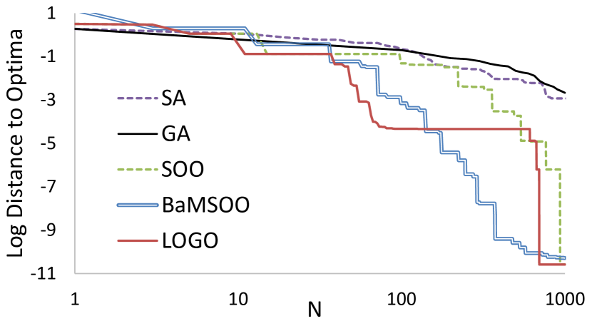
(f) Hartman 3

(g) Shekel 5

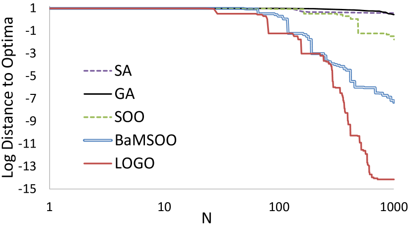
(h) Shekel 7

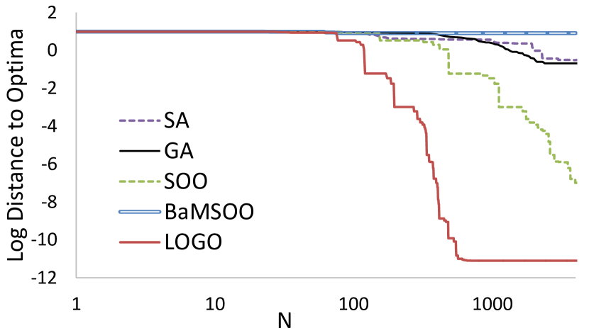
(i) Shekel 10

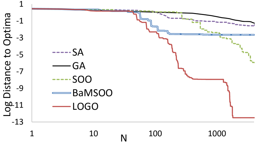
(j) Hartman 6

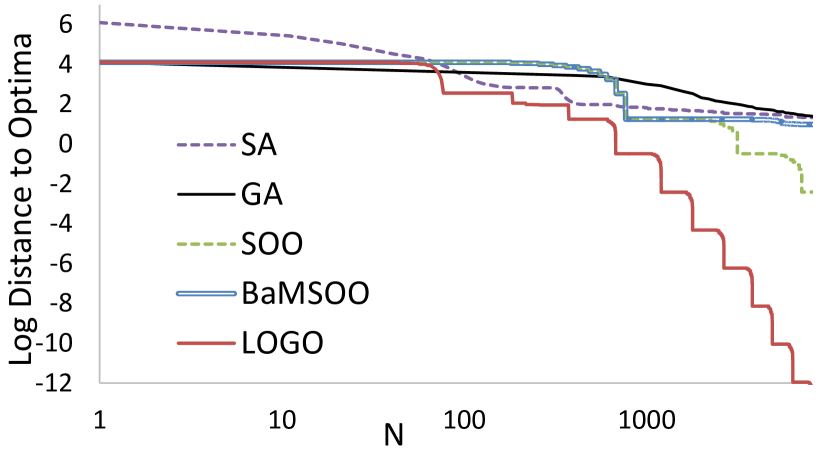
(k) Rosenbrock 10

Figure 5: Performance comparison: the number of evaluations $N$ vs. the log error computed as $\log_{10}\lvert f(x^{*})-f(x^{+})\rvert$. $f(x^{*})$ indicates the true optimal value of the objective function and $f(x^{+})$ is the best value determined by each algorithm.

 

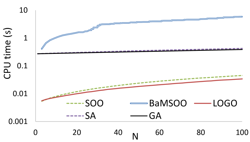
(a) Sin 1

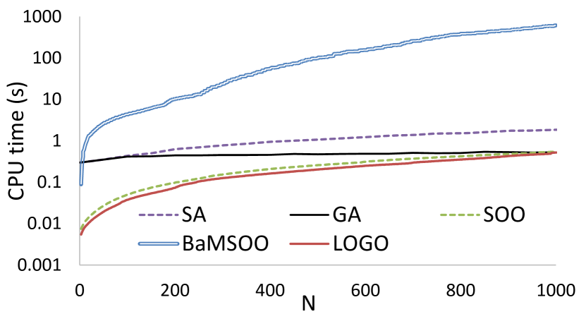
(b) Sin 2

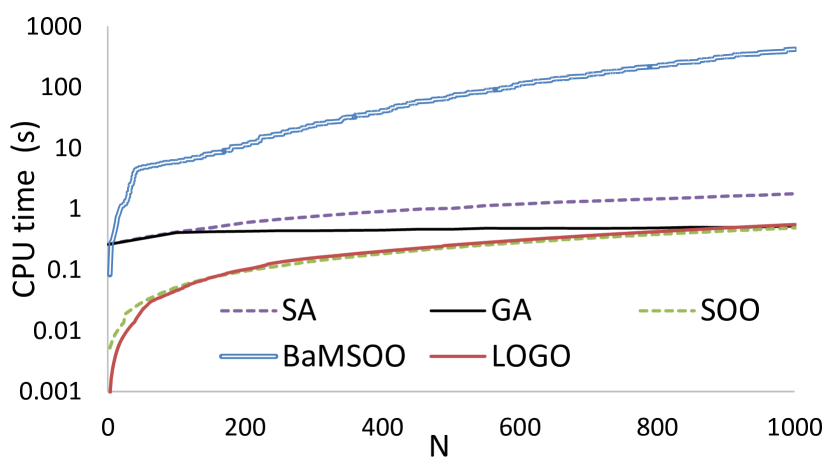
(c) Peaks

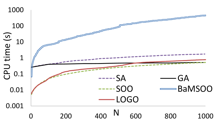
(d) Branin

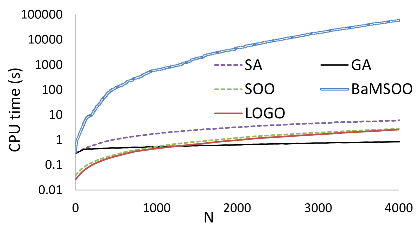
(e) Rosenbrock 2

(f) Hartman 3

(g) Shekel 5

(h) Shekel 7

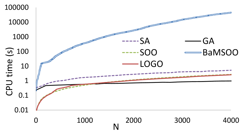
(i) Shekel 10

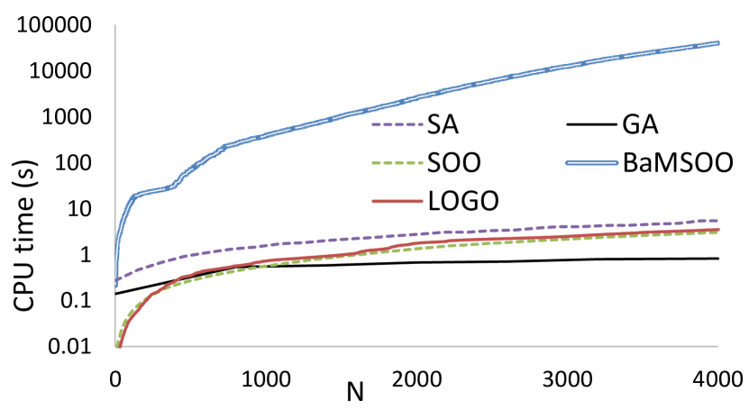
(j) Hartman 6

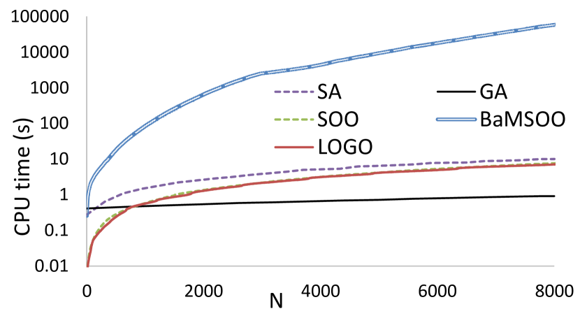
(k) Rosenbrock 10

Figure 6: CPU time comparison: CPU time required to achieve the performance indicated in Figure 5(k)

 

As illustrated in Figure 5(k), the LOGO algorithm generally delivered improved performance compared to the other algorithms. A particularly impressive result for the LOGO algorithm was its robustness for the more challenging functions, Shekel 10 and Rosenbrok 10. The function Shekel $m$ has $m$ local optimizers and the slope of the surface generally becomes larger as $m$ increases. Therefore, Shekel 10 and Rosenbrok 10, which have $10$-dimensionality, are generally more difficult functions when compared with the others in our experiment. Indeed, only the LOGO algorithm achieved acceptable performance on these. From Figure 6(k), we can see that the LOGO algorithm and the SOO algorithm were fast. The LOGO algorithm was often marginally slower than the SOO algorithm owing to the additional computation required to maintain the supersets. The reason why the BaMSOO algorithm required a large computational cost at some horizontal axis points is that it continued skipping to conduct the function evaluations (because the evaluations were judged to be not beneficial based on GP). This is an effective mechanism of BaMSOO to avoid wasteful function evaluations; however, one must be careful to make sure that the function evaluations are costly, relative to this mechanism.

In summary, compared to the BaMSOO algorithm, the LOGO algorithm was faster and considerably simpler (in both implementation and parameter selection) and had stronger theoretical bases while delivering superior performance in the experiments. When compared with the SOO algorithm, the LOGO algorithm decreased the theoretical convergence rate in the worst case analysis, but exhibited significant improvements in the experiments.

2pt Log Distance to Optimal [r] at 12 180 $N$ [t] at 270 25

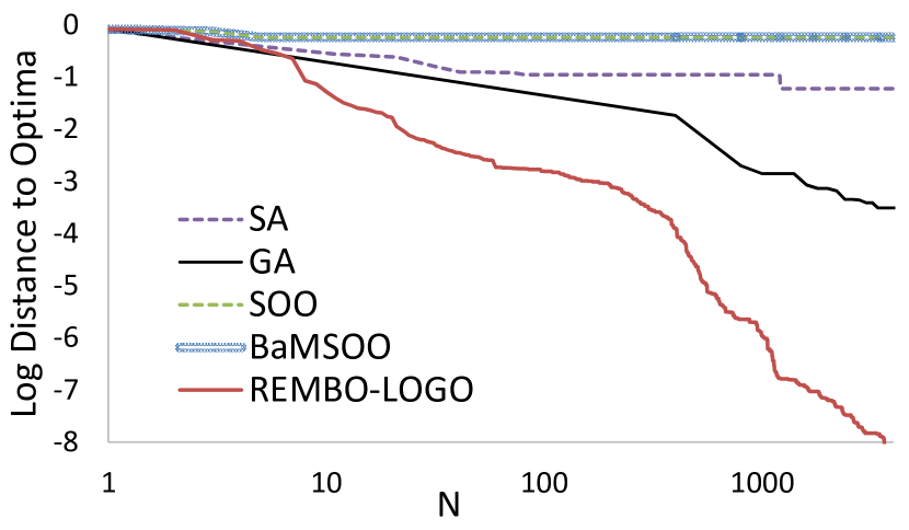
(a) Scalability: a 1000-dimensional function

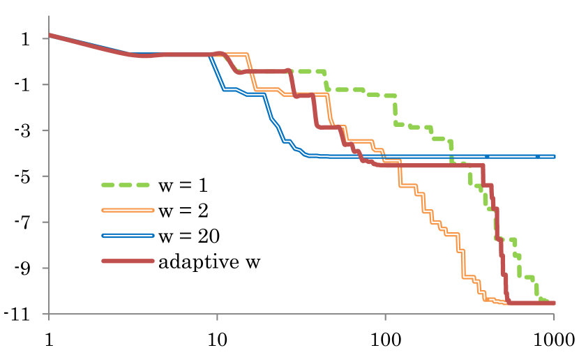
(b) Sensitivity to local bias parameter $w$

Figure 7: On the current possible limitations of LOGO

Now that we have confirmed the advantages of the LOGO algorithm, we discuss its possible limitations: scalability and parameter sensitivity. The scalability for high dimensions is a challenge for non-convex optimization in general as the search space grows exponentially in space. However, we may achieve the scalability by leveraging additional structures of the objective function that are present for some applications. For example, ? (?) showed an instance of deep learning models, in which the objective function has such an additional structure: the nonexistence of poor local minima. As an illustration, we combine LOGO with a random embedding method, REMBO (?), to account for another structure: a low effective dimensionality. In Figure 7 (a), we report the algorithms’ performances for a 1000 dimensional function: Sin 2 embedded in 1000 dimensions in the same manner described in Section 4.1 in the previous study (?).

Another possible limitation of LOGO is the sensitivity of its performance to the free parameter $w$. Even though we provided theoretical analysis and insight on the effect of the parameter value in the previous section, it is yet unclear how to set $w$ in a principle manner. We illustrate this current limitation in Figure 7 (b). The result labeled with “adaptive w” indicates the result with the fixed adaptive mechanisms of $w$ that we use in all the other experiments except ones in Figure 7 (b) and 8. In the illustration, we use the Branin function because the experiment conducted with it clearly illustrated the limitation. As can be seen in the figure, the performance in the early stage is always improved as $w$ increases because the algorithm finds a local optimum faster with higher $w$. However, if $w$ is too large, such as $w=20$ in the figure, the algorithm gets stuck at the local optimum for a long time. Thus, the best value (or sweet spot) exists between too large and too small values of $w$. In the results of this experiment, it can be seen that the choice of $w=2$ is the best, which finds the global optima with high precision within only $200$ function evaluations.

However, this limitation would not be a serious problem in practice for the following four reasons. First, a similar limitation exists, to the best of our knowledge, for any algorithms that are successfully used in practice (e.g., simulated annealing, genetic algorithm, swarm-based optimization, the DIRECT algorithm, and Bayesian optimization). Second, unlike any other previous algorithm, the finite-time loss bound always applies even for a bad choice of $w$. Third, we demonstrated in the previous experiments that a very simple adaptive rule may suffice to produce a good result. Also, future work may further mitigate this limitation by developing different methods to adaptively determine the value of $w$. Also, another possibility would be to conduct optimization over $w$ with a cheaper surrogate model. Finally, the limitation may not apply to some of the target objective functions at all.

For the fourth and final reason, recall that we speculated in the algorithm’s analysis that increasing $w$ would always have beneficial effects in some problems, as illustrated in Figure 4. Clearly, any problems within the scope of local optimization fall into this category. In Figure 8, we show a rather unobvious instance of such problems, and thus an example, for which the limitation of the parameter sensitivity does not apply. As can be seen in the diagram on the left in Figure 8, this test function has many local optima, only one of which is the global optimum. Nevertheless, as in the diagram on the right, the performance of the LOGO algorithm improves as $w$ increases, with no harmful effect.

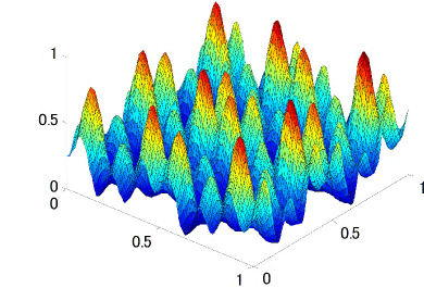
2pt $f$ [r] at -200 600 $x_{1}$ [tr] at 0 300 $x_{2}$ [t] at 400 330 2pt Log Distance to Optimal [r] at -160 420 Local Bias Parameter: $w$ [t] at 230 142

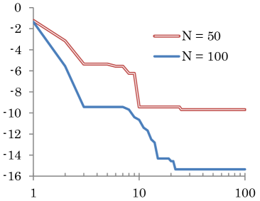
Figure 8: An example of problems where increasing $w$ is always better. The diagram on the left shows the objective function, and the diagram on the right presents the performance at $N=50$ and $100$ for each $w$.

6 Planning with LOGO via Policy Search

We now apply the LOGO algorithm to planning, which is an important area in the field of AI. The goal of our planning problem is to find an action sequence that maximizes the total return over the infinite discounted horizon or finite horizon (unlike classical planning problem, we do not consider constraints that specify the goal state). In this paper, we discuss the formulations for the case of the infinite discounted horizon, but all the arguments are applicable to the case of a finite horizon with straightforward modifications. We consider the case where the state/action space is continuous, the planning horizon is long, and the transition and reward functions are known and deterministic.

The planning problem can be formulated as follows. Let $S\subset\mathbb{R}^{D_{S}}$ be a set of states, $A\subset\mathbb{R}^{D_{A}}$ be a set of actions, $T\colon\mathbb{R}^{D_{S}}\to\mathbb{R}^{D_{S}}$ be a transition function, $R\colon\mathbb{R}^{D_{S}}\times\mathbb{R}^{D_{A}}\to\mathbb{R}$ be a return or reward function, and $\gamma\leq 1$ be a discount factor. A planner considers to take an action $a\in A$ in a state $s\in S$, which triggers a transition to another state based on the transition function $T$, while receiving a return based on the reward function $R$. The discount factor $\gamma$ discounts the future rewards to fulfill either or both of the following two roles: accounting for the relative importance of immediate rewards compared to future rewards, and obviating the need to think ahead toward the infinite horizon. An action sequence can be represented by a policy $\pi$ that maps the state space to the action space: $\pi\colon\mathbb{R}^{D_{S}}\to\mathbb{R}^{D_{A}}$.

The value of an action sequence or a policy $\pi$, $V^{\pi}$, is the sum of the rewards over the infinite discounted horizon, which is

$$V^{\pi}(s_{0})=\sum_{j=0}^{\infty}\gamma^{t}R(s_{j},\pi(s_{j})).$$

The value of a policy can be also written with a recursive form as

$$V^{\pi}(s)=R(s,\pi(s))+\gamma V^{\pi}\bigl{(}T(s,\pi(s))\bigr{)}.$$ (2)

Here, we are interested in finding the optimal policy $\pi^{*}$. In the dynamic programing approach, we can compute the optimal policy, by solving the following Bellman’s optimality equation:

$$V^{*}(s)=\max_{a}R(s,a)+\gamma V^{*}(T(s,a))$$ (3)

where $V^{*}$ is the value of the optimal policy. In Equation (3), the optimal policy $\pi^{*}$ is the set of the actions defined by the max. A major problem with this approach is that the efficiency of the computation depends on the size of the state space. In a real-world application, the state space is usually very large or continuous, which often makes it impractical to solve Equation (3).

A successful approach to avoid the state size dependency is to focus only on the state space that is reachable from the current state within the planning time horizon. In this way, even with an infinitely large state space, a planner only needs to consider a finitely sized subset of the space. This approach is called local planning. Unlike local optimization vs. global optimization, the optimal solution of local planning is indeed globally optimal, given the initial state. It is called local planning because it does not cover all the states and its solution changes for different initial states. Accordingly, as the initial state changes, a planner may need to conduct re-planning.

A natural way to solve local planning is to use tree search methods, which construct a tree rooted in an initial state toward the future possible states in the depth of the planning horizon. This tree search can be conducted using any traditional search method, including both uninformed search (e.g., breadth-first and depth-first search) and informed (heuristic) search (e.g., $\rm A^{*}$ search). Also, recent studies have developed several tree-based algorithms that are specialized to local planning. Among those, the SOO algorithm, the direct predecessor of the LOGO algorithm, was applied to local planning with the tree search approach (?). Most of the new algorithms, for example, HOLOP (?, ?), operate with stochastic transition functions.

However efficient these proposed algorithms are, the search space in the tree search approach grows exponentially in the planning time horizon, $H$. Therefore, local planning with the tree search approach would not work well with a very long time horizon. In some applications, a small $H$ is justified, but in other applications, it is not. If an application problem requires a long time tradeoff between immediate and future rewards, then the tree search approach would be impractical. Here, we are motivated to solve such a real-world application, and therefore need another approach.

In this paper, we consider policy search (?) as an effective alternative to solve the planning problem with continuous state/action space and with a long time horizon. Policy search is a form of local planning. Thus, like the tree search approach, it operates even with infinitely large or continuous state space. In addition, unlike the tree search approach, policy search significantly reduces the search space by naturally integrating the domain-specific expert knowledge into the structure of the policy. More concretely, the search space of policy search is a set of policies $\{\pi_{x}:x\in\Omega\}$, which are parameterized by a vector $x$ in $\Omega\subset\mathbb{R}^{D}$. Therefore, the search space is no longer dependent on the planning time horizon $H$, the state space $S$, nor the action space $A$, but only on the parameter space $\Omega$. Here, parameter space $\Omega$ can be determined by expert knowledge, which can significantly reduce the search space.

We use the regret $r_{m}$ as the measure of the policy search algorithm’s performance:

$$r_{m}=V^{\pi_{x}^{*}}(s_{0})-V^{\pi_{x}^{+}(m)}(s_{0})$$

where $\pi_{x}^{*}$ is the optimal policy in the given set of policies $\{\pi_{x}:x\in\Omega\}$, and $\pi_{x}^{+}(m)$ is the best policy found by an algorithm after the $m$ steps of planning. An evaluation of each policy takes $mH$ steps if we consider a fixed planning horizon $H$. Here, $\pi_{x}^{*}$ may differ from the optimal policy $\pi^{*}$ when $\pi^{*}$ is not covered in the set $\{\pi_{x}:x\in\Omega\}$.

The policy search approach is usually adopted with gradient methods (?, ?, ?). While a gradient method is fast, it converges to local optima (?). Further, it has been observed that it may result in a mere random walk when large plateaus exist in the surface of the policy space (?). Clearly, these problems can be resolved using global optimization methods at the cost of scalability (?, ?). Unlike previous policy search methods, our method guarantees finite-time regret bounds w.r.t. global optima in $\{\pi_{x}:x\in\Omega\}$ without strong additional assumption, and provides a practically useful convergence speed.

6.1 LOGO-OP Algorithm: Leverage (Unknown) Smoothness in Both Policy Space and Planning Horizon

In this section, we present a simple modification of the LOGO algorithm to leverage not only the unknown smoothness in policy space but also the known smoothness over the planning horizon. The former is accomplished by the direct application of the LOGO algorithm to policy search, and the latter is what the modification in this section aims to do without losing the advantage of the original LOGO algorithm. We call the modified version, Locally Oriented Global Optimization with Optimism in Planning horizon (LOGO-OP). As a result of this modification, we add a new free parameter $L$.

The pseudocode for the LOGO-OP algorithm is provided in Algorithm 2. By comparing Algorithms 1 and 2, it can be seen that the LOGO-OP algorithm functions in the same manner as the LOGO algorithm, except for line 15 (the function evaluation or, equivalently, the policy evaluation in the policy search) and line 20. Notice that the LOGO algorithm is directly applicable to the policy search by considering $V$ to be $f$ in Algorithm 1. While the LOGO algorithm does not assume the structure of the function $f$, the LOGO-OP algorithm functions with and exploits the given structure of the value function $V$ (i.e., MDP model). The algorithm functions as follows. The policy evaluation is performed for each policy $\pi_{x}$ with a parameter $x$ specified by each of the two new hyperrectangles (from line 15-1 to 15-11). Given the initial condition $s_{0}\in S$, the transition function $T$, the reward function $R$, a discount factor $\gamma\leq 1$, and the policy $\pi_{x}$, the algorithm computes the value of the policy as in Equation (2) (from line 15-2 to line 15-10, except line 15-6).

The main modification appears in line 15-6 where the algorithm leverages the known smoothness over the planning horizon. Remember that the unknown smoothness in policy space (or input space $x$) is specified as $f(x^{*})-f(x)\leq\ell(x,x^{*})$ (from Assumption 1) and thus it infers the upper bound of the value of a policy that is not yet evaluated but similar (close in policy space w.r.t. $\ell$) to already evaluated polices. Conversely, the known smoothness over the planning horizon renders the upper bound on the value of a policy while the particular policy is being evaluated. That is, the known smoothness over the planning horizon can be written as

$$\sum_{j=0}^{\infty}\gamma^{j}R(s_{j},\pi_{x}(s_{j}))-\sum_{j=0}^{t}\gamma^{j}R(s_{j},\pi_{x}(s_{j}))\leq\frac{\gamma^{t+1}}{1-\gamma}R_{\mathit{max}}$$

where $0\leq t\leq\infty$ is a arbitrary point in the planning horizon as in line 15-3 and $R_{\mathit{max}}$ is the maximum reward. This known smoothness is due to the definition of $R_{\mathit{max}}$ and the sum of a geometric series. In the case of the finite horizon with $H$, we have the same formula with $(\gamma^{t}/(1-\gamma))R_{\mathit{max}}$ being replaced by $(H-t)R_{\mathit{max}}$. In line 15-6, unlike the original LOGO algorithm, the LOGO-OP algorithm terminates the evaluation of a policy when the continuation of evaluating the policy is judged to be a misuse of the computational resources based on the known smoothness over the planning horizon. Concretely, it terminates the evaluation of a policy when the upper bound of the value of the policy becomes less than $(V^{+}-L)$, where $V^{+}$ is the value of the best policy found thus far and $L$ is the algorithm’s parameter.

When the upper bound of the value of policy becomes less than $V^{+}$, the planner can know that the policy is not the best policy. Thus, it is tempting to simply terminate the policy evaluation with this criterion. However, the essence of the LOGO algorithm is the utilization of the unknown smoothness embedded in the surface of the value function in the policy space. In other words, the algorithm makes use of the result of each policy evaluation, whether the policy is the best one or not. Any interruption of the policy evaluation changes the shape of the surface of the value function, which interferes with the mechanism of the LOGO algorithm. Nevertheless, the some degree of the interruption is likely to be beneficial since our goal is to find the optimal policy instead of surface analysis.

Algorithm 2 LOGO-OP algorithm

0:Inputs (problem): the initial condition $s_{0}\in S$, the transition function $T$, the reward function $R$, a discount factor $\gamma\leq 1$ with convergence criteria (or finite horizon $H$), the policy space $\pi_{x}:x\in\Omega\subset\mathbb{R}^{D}$.

1:Inputs (parameter): the search depth function $h_{\mathit{max}}\colon\mathbb{Z}^{+}\to[1,\infty)$, the local weight $w\in\mathbb{Z}^{+}$, stopping condition, the maximum reward $R_{\mathit{max}}$, a parameter $L$.

2–5:lines 2–5 are exactly the same as lines 2–5 in Algorithm 1

6:Adds the initial hyperrectangle $\Omega^{\prime}$ to the set: $\psi_{0}\leftarrow\psi_{0}\cup\{\Omega^{\prime}\}$ (i.e., $\omega_{0,0}=\Omega^{\prime}$)

7:Evaluate the value function $V$ at the center point of $\Omega^{\prime}$, $c_{0,0}$: $\mathit{val}[\omega_{0,0}]\leftarrow V(c_{0,0})$, $V^{+}\leftarrow\mathit{val}[\omega_{0,0}]$

8:for iteration ${}=1,2,3,\dots$ 

9:   $\mathit{val}_{\mathit{max}}\leftarrow-\infty$, $h_{\mathit{plus}}\leftarrow h_{\mathit{upper}}$

10:   for $k=0,1,2,\dots,\max(\lfloor\min(h_{\mathit{max}}(n),h_{\mathit{upper}})/w\rfloor,h_{\mathit{plus}})$ 

11:     Select a hyperrectangle to be divided: $(h,i)\in\arg\max_{h,i}\mathit{val}[\omega_{h,i}]$ for $h,i:\omega_{h,i}\in\Psi_{k}$

12:     if $\mathit{val}[\omega_{h,i}]>\mathit{val}_{\mathit{max}}$ then

13:       $\mathit{val}_{\mathit{max}}\leftarrow\mathit{val}[\omega_{h,i}]$, $h_{\mathit{plus}}\leftarrow 0$, $h_{\mathit{upper}}\leftarrow\max(h_{\mathit{upper}},h+1)$, $n\leftarrow n+1$

14:       Divide this hyperrectangle $\omega_{h,i}$ along the longest coordinate direction

15:     

- three smaller hyperrectangles are created $\rightarrow$ $\omega_{\mathit{left}}$, $\omega_{\mathit{center}}$, $\omega_{\mathit{right}}$

- $\mathit{val}[\omega_{\mathit{center}}]\leftarrow\mathit{val}[\omega_{h,i}]$

16:       Evaluate the value function $V$ at the center points of the two new hyperrectangles:

            16–1:       for each policy $\pi_{x}$ corresponding $c_{\omega_{\mathit{left}}}$ and $c_{\omega_{\mathit{right}}}$ 

            16–2:         $z_{1}\leftarrow 0$, $z_{2}\leftarrow 1$, $s\leftarrow s_{0}$

            16–3:         for $t=0,1,2,\dots$, 

            16–4:           $z_{1}\leftarrow z_{1}+z_{2}R(s,\pi_{x}(s))$

            16–5:           $z_{2}\leftarrow\gamma z_{2}$, $s\leftarrow T(s,\pi_{x}(s))$ ,

            16–6:           if $z_{1}+(\gamma^{t+1}/(1-\gamma))R_{\mathit{max}}<(V^{+}-L)$ then Exit loop

            16–7:           if convergence criteria is met then Exit loop

            16–8:         end for

            16–9:         save $z_{1}$ as the value of the corresponding rectangle

            16–10:         $\mathit{val}[\omega_{\mathit{left}}]\leftarrow z_{1}$ or $\mathit{val}[\omega_{\mathit{right}}]\leftarrow z_{1}$

            16–11:       end for

            16–12:       $V^{+}\leftarrow\max(V^{+},\mathit{val}[\omega_{\mathit{left}}],\mathit{val}[\omega_{\mathit{center}}],\mathit{val}[\omega_{\mathit{right}}])$

17:       Group the new hyperrectangles into the set $h+1$ and remove the original rectangle: $\psi_{h+1}\leftarrow\psi_{h+1}\cup\{\omega_{\mathit{center}},\omega_{\mathit{left}},\omega_{\mathit{right}}\},\quad\psi_{h}\leftarrow\psi_{h}\setminus\omega_{h,i}$

18:     end if

19:     if stopping condition is met then Return $(h,i)=\arg\max_{h,i}\mathit{val}[\omega_{h,i}]$

20:   end for

21:   for all intervals $\omega$ with $\mathit{val}[\omega]<(V^{+}-L)$ do $\mathit{val}[\omega]\leftarrow(V^{+}-L)$

22:end for

The LOGO-OP algorithm uses $L$ to determine the degree of the interruption. Because $V^{+}$ is monotonically increasing along the execution, the value of a policy that is not fully evaluated owing to line 15-6 in early iterations tends to be greater than the value of a policy that is not fully evaluated in the later iterations. The algorithm resolves this problem in line 20 such that it is not biased to divide the interval evaluated in an early iteration.

With smaller $L$, the LOGO-OP algorithm can stop the evaluation of a non-optimal policy earlier, at the cost of accuracy in the evaluation of the value function’s surface. With larger $L$, the algorithm needs to spend more time on the evaluation of a non-optimal policy, but can obtain a more accurate estimate of the value function’s surface. In the regret analysis, we show that a certain choice of $L$ ensures a tighter regret bound when compared to the direct application of the LOGO algorithm.

6.2 A Parallel Version of the LOGO-OP Algorithm

The LOGO-OP algorithm presented in Algorithm 2 has four main procedures: Select (line 11), Divide (line 14), Evaluate (line 15), and Group (line 16). A natural way to parallelize the algorithm is to decouple Select from the other three procedures. That is, let the algorithm first Select $z$ hyperrectangles to be divided, and then allocate the $z$ number of Divide, Evaluate, and Group to $z$ parallel workers. However, this natural parallelization has data dependency from one Select to another Select. In other words, the procedure of the next Select cannot start before Divide, Evaluate, and Group for the previous Select are finalized. As a result, the parallel overhead tends to be non-negligible. In addition, if Select chooses less hyperrectangles than parallel workers, then the available resources of the parallel workers are wasted. Indeed, the latter problem was tackled by creating multiple initial rectangles in a recent parallelization study of the DIRECT algorithm (?). While the use of multiple initial rectangles can certainly mitigate the problem, it still allows the occasional occurrence of the resource wastage, in addition to requiring the user to specify the arrangement of the initial rectangles.

To solve these problems, we instead decouple the Evaluate procedure from the other three procedures and allocate only the Evaluate task to each parallel worker. We call the parallel version, the pLOGO-OP algorithm. The algorithm uses one master process to conduct Select, Divide, and Group operations and an arbitrary number of parallel workers to execute Evaluate. The main idea is to temporarily use the artificial value assignment to the center point of a hyperrectangle in the master process, which is overwritten by the true value when the parallel worker finishes evaluating the center point. With this strategy, there is no data dependency and all the parallel workers are occupied with tasks almost all the time. In this paper, we use the center value of the original hyperrectangle before division as the temporary artificial value, but the artificial value may be computed using a more advanced method (e.g., methods in surface analysis) in future work. For the center point of the initial hyperrectangle, we simply assign the worst possible value (if we have no knowledge regarding the worst value, we can use $-\infty$).

The master process keeps selecting new hyperrectangles unless all the parallel workers are occupied with tasks. This logic ensures that all the parallel workers always have tasks assigned by the master process, but the master process does not select too many hyperrectangles based on the artificial information. Note that this parallelization makes sense only when Evaluate is the most time consuming procedure, and it is very likely true for policy evaluation.

6.3 Regret Analysis

Under a certain condition, all the finite-loss bounds of the LOGO algorithm are directly translated to the regret bound of the LOGO-OP algorithm. The condition that must be met is that $(V^{+}-L)$ is less than the center value of the optimal hyperinterval during the algorithm’s execution. We state the regret bound more concretely below. For simplicity, we use the notion of a planning horizon $H$, which is the effective (non-negligible) planning horizon for LOGO in accordance with the discount factor, $\gamma$. Let $H^{\prime}$ be the effective planning horizon of the LOGO-OP algorithm. Then, the planning horizon for LOGO-OP, $H^{\prime}$, becomes smaller than that for LOGO, $H$, as the algorithm finds improved function values. This is because the LOGO-OP algorithm terminates each policy evaluation at line 15-6 when the upper bound on the policy value is determined to be lower than $(V^{+}-L)$.

Corollary 3.

Let $H^{\prime}\leq H$ be the planning horizon used by the LOGO-OP algorithm at each policy evaluation. Let $V^{+}$ be the value of the best policy found by the algorithm at any iteration. Assume that the value function of the policy satisfies Assumptions 1 and B1. If $(V^{+}-L)$ is maintained to be less than the center value of the optimal hyperinterval, then the algorithm holds the finite-time loss bound of Theorem 2 with

$$n\geq\biggl{\lfloor}\frac{m}{2H^{\prime}}\biggr{\rfloor}.$$

Proof.

As the policy search is just a special case of the optimization problem, it is trivial that the loss bound of Theorem 2 holds for the LOGO algorithm when it is applied to policy search. Because every function evaluation takes $H$ steps in the planning horizon, we have $n\geq\lfloor m/2H\rfloor$ in this case. For the LOGO-OP algorithm, only the effect that new parameter $L$ has in the loss analysis takes place in the proof of Lemma 2. If $(V^{+}-L)$ is maintained to be less than the center value of the optimal interval, then all the statements in the proof hold true for the LOGO-OP algorithm as well. Here, due the effect of $L$, function evaluation may take less than $H$ steps in the planning horizon. Therefore, we have the statement of this corollary. ∎

We can tighten the regret bound of the LOGO-OP algorithm by decreasing $L$, since the algorithm can then terminate evaluations of unpromising policies earlier, which means that the value of $H^{\prime}$ in the bound is reduced. However, using a too small value of $L$ that violates the condition in Corollary 3 leads us to discard the theoretical guarantee. Even in that case, because the too small value of $L$ only results in a more global search, the consistency property, $\lim_{n\to\infty}r_{n}=0$, is still trivially maintained. On the other hand, if we set $L=\infty$, the LOGO-OP algorithm becomes equivalent to the direct application of the LOGO algorithm to policy search, and thus, we have the regret bound of Corollary 3 with $H^{\prime}=H$.

The pLOGO-OP algorithm also maintains the same regret bound with $n=n_{p}$ where $n_{p}$ counts the number of the total divisions that are devoted to the set of $\delta$-optimal hyperinterval $\psi_{kw+l}(l+1)^{*}$, where $(w-1)\geq l\geq 0$. While non-parallel versions ensure the devotion to $\psi_{kw+l}(l+1)^{*}$, the parallelization makes it possible to conduct division on other hyperintervals. Thus, considering the worst case, the pLOGO-OP may not improve the bound in our proof procedure, although the parallelization is likely beneficial in practice.

6.4 Application Study on Nuclear Accident Management

The management of the risk of potentially hazardous complex systems, such as nuclear power plants, is a major challenge in modern society. In this section, we apply the proposed method to accident management of nuclear power plants and demonstrate the potential utility and usage of our method in a real-world application. Our focus is on assessing the efficiency of containment venting as an accident management measure and on obtaining knowledge about its effective operational procedure (i.e., policy $\pi$). This problem requires planning with continuous state space and with a very long planning horizon ($H\geq 86400$), for which dynamic programming (e.g., value iteration), tree-based planning (e.g., $\rm A^{*}$ search and its variants) would not work well (dynamic programming suffers from the curse of dimensionality for the state space, and the search space of tree-based methods grows exponentially in the planning horizon).

Containment venting is an operation that is used to maintain the integrity of the containment vessel and to mitigate accident consequences by releasing gases from the containment vessel to the atmosphere. In the accident at the Fukushima Daiichi nuclear power plant in 2011, the containment venting was activated as an essential accident management measure. As a result, in 2012, the United States Nuclear Regulatory Commission (USNRC) issued an order for $31$ nuclear power plants to install the containment vent system (?). Currently, many countries are considering the improvement of the containment venting system and its operational procedures (?). The difficulty of determining its actual benefit and effective operation comes from the fact that the containment venting also releases fission products (radioactive materials) into the atmosphere. In other words, the effective containment venting must trade off the future risk of containment failure against the immediate release of fission products (radioactive materials). In our experiments, we use the release amount of the main fission product compound, cesium iodide (CsI), as a measure of the effectiveness of the containment venting.

In the nuclear accident management literature, an integrated physics simulator is used as the model of world dynamics or the transition function $T$ and the state space $S$. The simulator that we adopt in this paper is THALES2 (Thermal Hydraulics and radionuclide behavior Analysis of Light water reactor to Estimate Source terms under severe accident conditions) (?). Thus, the transition function $T$ and the state space $S$ are fully specified by THALES2. The initial condition $s_{0}\in S$ is designed to approximately simulate the accident at the Fukushima Daiichi nuclear power plant. In this experiment, we focus on a single initial condition with the deterministic simulator, the relaxation of which is discussed in the next section. The reward function $R$ is the negative of the amount of CsI being released in the atmosphere as a result of a state-action pair. We use the finite-time horizon $H=86400$ seconds ($24$ hours), which is a traditional first phase time-window considered in risk analysis with nuclear power plant simulations (owing to the assumption that after $24$ hours, many highly uncertain human operations are expected). We use the following policy structure based on our engineering judgment.

$$\pi_{x}=\begin{cases}1&\text{if }((\mathit{FP}\leq x_{1})\cap(\mathit{Press}\geq x_{2}))\cup(\mathit{Press}>100490),\\ 0&\text{otherwise},\end{cases}$$

where $\pi_{x}=1$ indicates the implementation of the containment venting, $\mathit{FP}$ (g) represents the amount of CsI in the gas phase of the suppression chamber, and $\mathit{Press}$ (kgf/m²) is the pressure of the suppression chamber. Here, the suppression chamber is the volume in the containment vessel that is connected to the atmosphere via the containment venting system. This policy structure reflects our engineering knowledge that the venting should be done while the fission products exist under a certain amount in the suppression chamber, but should not be operated before the pressure gets larger than a specific value. We consider $x_{1}=[0,3000]$ and $x_{2}=[10810,100490]$. We let $\pi_{x}=1$ whenever the pressure exceeds $100490$ kgf/m², since the containment failure is considered to probably occur after the pressure exceeds this point. The detail of the experimental setting is outlined in Appendix A.

We first compare the performance of various algorithms in this problem. For all the algorithms, we used the same parameter settings as in the benchmark tests in Section 5. That is, we used $h_{\mathit{max}}(n)=w\sqrt{n}-w$ and a simple adaptive procedure for the parameter $w$ with $W=\{3,4,5,6,8,30\}$. For the LOGO-OP algorithm and the pLOGO-OP algorithm, we blindly set $L=1000$ (i.e., there is likely a better parameter setting for $L$). We used only eight parallel workers for the pLOGO-OP algorithm.

2pt CsI release by the Computed Policy (g) [r] at 0 100 Wall time (s) [t] at 160 0

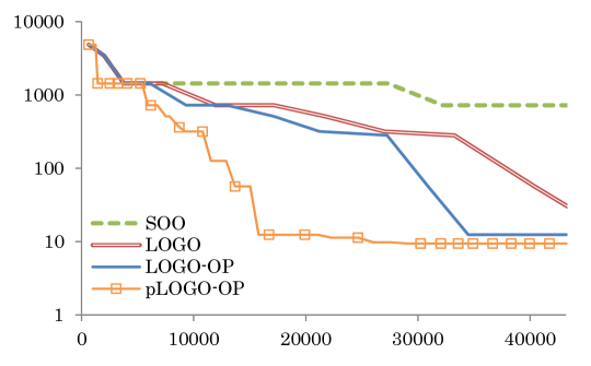
Figure 9: Performance of the computed policy (CsI release) vs. Wall Time.

Figure 9 shows the result of the comparison with wall time $\leq 12$ hours. The vertical axis is the total amount of CsI released into the atmosphere (g), which we want to minimize. Since we conducted containment venting whenever the pressure exceeded $100490$ kgf/m², containment failure was prevented in all the simulation experiments. Thus, the lower the value along the vertical axis gets, the better the algorithm’s performances is. As can be seen, the new algorithms performed well compared to the SOO algorithm. It is also clear that the two modified versions of the LOGO algorithm improved the performance of the original. For the LOGO-OP algorithm, the effect of $L$ on the computational efficiency becomes greater as the found best policy improves. Indeed, the LOGO algorithm required $10798$ seconds for ten policy evaluations and $52329$ seconds for $48$ evaluations. The LOGO-OP algorithm required $9297$ seconds for ten policy evaluations, and $44678$ seconds for $48$ evaluations. This data in conjunction with Figure 9 illustrates the property of the LOGO-OP algorithm that the policy evaluation becomes faster as the found best policy improves. For the pLOGO-OP algorithm, the number of function evaluations performed by the algorithm increased by a factor of approximately eight (the number of parallel workers) compared to the non-parallel versions. Notice that the parallel version tends to allocate the extra resources to the global search (as opposed to the local search). We can focus more on the local search by utilizing the previous results of the policy evaluations; however, the parallel version must initiate several policy evaluations without waiting for the previous evaluations, resulting in a tendency for global search. This tendency forced the improvement, in terms of reducing the amount of CsI, to be moderate relative to the number of policy evaluations in this particular experiment. However, such a tendency may have a more positive effect in different problems where increased global search is beneficial. The CPU time per policy evaluation varied significantly for different policies owing to the different phenomenon computed in the simulator. On the average, for the LOGO-OP algorithm, it took approximately $930$ seconds per policy evaluation.

Now that we partially confirmed the validity of the pLOGO-OP algorithm, we attempt to use it to provide meaningful information to this application field. Based on the examination of the results in the above comparison, we narrowed the range of the parameter values as $x_{1}=[0,1.2]$ and $x_{2}=[10330,10910]$. After the computation with CPU time of $86400$ (s) and with eight workers for the parallelization, the pLOGO-OP algorithm found the policy with $x_{1}\approx 0.195$ (g) and $x_{2}\approx 10880$ (kgf/m²). With the policy determined, containment failure was prevented and the total amount of CsI released into the atmosphere was limited to approximately $0.5$ (g) (approximately $0.002\%$ of the total CsI) in the $24$ hours after the initiation of the accident. This is a major improvement because this scenario with our experimental setting is considered to result in a containment failure or at best, in a large amount of CsI release, more than $2000$ (g) (about $10\%$ of total CsI) in our setting. The computational cost of CPU time of $86400$ (s) is likely acceptable in the application field. In terms of computational cost, we must consider two factors: the offline computation and the variation of scenarios. The computational cost with CPU time of $86400$ (s) for a phenomenon that requires $86400$ (s) is not acceptable for online computation (i.e., determining a satisfactory policy while the accident is progressing). However, such computational cost is likely acceptable if we consider preparing acceptable policies for various scenarios in an offline manner (i.e., determining satisfactory polices before the accident). Such information regarding these polices can be utilized during an accident by first identifying the accident scenario with heuristics or machine learning methods (?). For offline preparation, we must determine policies for various major scenarios and thus if each computation takes, for example, one month, it may not be acceptable.

2pt Venting (-) / CsI (g) [r] at -10 80 Time along Accident Progression (s) [t] at 230 -5

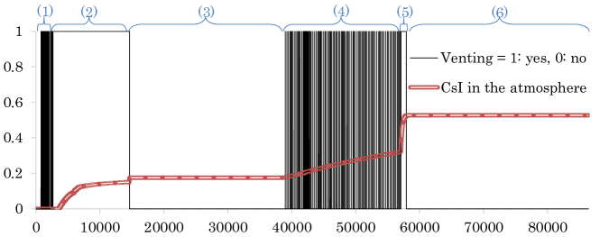
Figure 10: Action sequence generated by found policy and CsI release

Note that the policy found by our method is both novel and nontrivial in the literature, and yet worked very well. Accordingly, we explain why the policy performed as well as it did. Figure 10 shows the action sequence generated by the policy found and the amount of CsI (g) released versus accident progression time (s). We analyze the action sequence by dividing it into six phases, as indicated in Figure 10, with the six numbers inside the parentheses. In the first phase (1), the venting is conducted intermittently in order to keep the pressure around $x_{2}\approx 10880$ (kgf/m²). In this phase, no fission product has yet been released from the nuclear fuels. Reducing the pressure and the heat should be done preferably without releasing fission products, and the actions in this phase accomplish this. One may wonder why the venting should be done intermittently, instead of continuing to conduct venting to reduce the pressure as much as possible, which can be done without the release of fission products only in this phase. This is because reducing the pressure too much leads to a large difference between the pressures in the suppression chamber and the reactor pressure vessel, which in turn results in a large mass flow and fission product transportation from the reactor pressure vessel to the suppression chamber (see Figure 11 in Appendix A for information about the mass flow paths). The increase in the amount of fission products in the suppression chamber will likely result in a large release of fission products into the atmosphere when venting is conducted. Therefore, this specific value of $x_{2}$ that generates the intermittent venting works well in the first phase. In the second phase (2), containment venting is executed all the time since the pressure in the suppression chamber increases rapidly in this phase (due to the operation of depressurizing the reactor pressure vessel via the SRV line), and thus, the criterion ($\mathit{Press}\geq x_{2}$) in the policy is satisfied all the time from this point. In the beginning of the third phase (3), the amount of CsI in the suppression chamber exceeds $x_{1}\approx 0.195$ (g) and thereby no venting is conducted. In the fourth phase (4), the pressure reaches $100490$ (kgf/m²) and containment venting is intermittently done in order to keep the pressure under the point to avoid catastrophic containment failure. In the fifth phase (5), the containment vent is kept open because the amount of CsI in the gas phase of the suppression chamber decreases to below $x_{1}$ (due to the phenomenon illustrated in Figure 12 in Appendix A). This continuous containment venting decreases the pressure such that no venting is required in terms of the pressure in the final phase (6), where venting is not conducted also because the amount of CsI becomes larger than $x_{1}$.

Thus, it is clear that the policy found by this AI-related method also has a basis in terms of physical phenomenon. In addition, the generated action sequence is likely not simple enough for an engineer to discover with several sensitivity analyses. In particular, not only did our method solve the known tradeoff between the immediate CsI release and the risk of future containment failure, the method also discovered the existence of a new tradeoff between the immediate reduction of the pressure without CsI release and future increase in the mass flow. Although there is no consensus as to how to operate the containment venting system at the moment, the tendency is to use it only when the pressure exceeds a certain point in order to prevent immediate sever damage of containment vessel, which corresponds only to the fourth phase (4) in Figure 10. In our experiment, such a myopic operation resulted in containment failure, or a significantly large amount of CsI being released into the atmosphere (at least more than $4800$ (g)).

In summary, we successfully applied the proposed method to investigate the containment venting policy in nuclear power plant accidents. As a preliminary application study, several topics are left to future work. From a theoretical viewpoint, future work should consider a way to mitigate the simulation bias due to model error and model uncertainty. For the model error, the robotics community is already cognizant that a small error in a simulator can result in poor performance of the derived policy (i.e., simulation bias) (?). We can mitigate this problem by adding a small noise to the model, since the noise works as regularization to prevent over-fitting as demonstrated by ? (?). For the model uncertainty, recent studies in the field of nuclear accident analysis provide possible directions for the treatment of uncertainty in accident phenomena (?) and accident scenarios (?). As a result of either or both of these countermeasures, the objective function becomes stochastic, and thereby we may first expand the pLOGO-OP algorithm to stochastic case. On the other hand, from the phenomenological point of view, future work should consider other fission products as well as CsI. Such fission products include, but are not limited to, Xe, Cs, I, Te, Sr, and Ru. In particular, a noble gas element, such as Xe, can be a major concern in an accident (it tends to be released a lot and is easily diffused into the atmosphere), but its property is different from CsI (its half-life is much smaller). Thus, if Xe is identified as a major concern, one may consider a significantly different policy from ours (considering its half-life, one may delay conducting the containment venting).

7 Conclusions

In this paper, we proposed the LOGO algorithm, the global optimization algorithm that is designed to operate well in practice while maintaining a finite-loss bound with no strong additional assumption. The analysis of the LOGO algorithm generalized previous finite-loss bound analysis. Importantly, the analysis also provided several insights regarding practical usage of this type of algorithm by showing the relationship among the loss bound, the division strategy, and the algorithm’s parameters.

We applied the LOGO algorithm to an AI planning problem with the policy search framework, and showed that the performance of the algorithm can be improved by leveraging not only the unknown smoothness in policy space, but also the known smoothness in the planning horizon. As our study is motivated to solve real-world engineering applications, we also discussed a parallelization design that utilizes the property of AI planning in order to minimize the overhead. The resulting algorithm, the pLOGO-OP algorithm, was successfully applied to a complex engineering problem, namely, policy derivation for nuclear accident management.

Aside from the planning problem that we considered, the LOGO algorithm can be also used, for example, to optimize parameters of other algorithms (i.e., algorithm configuration). In the AI community, the algorithm configuration problem has been addressed by several methods, including a genetic algorithm (?), discrete optimization with convergence guarantee in the limit (?), the racing approach originated from the machine learning community (Hoeffding Races) (?), model-based optimization with convergence guarantee in the limit (?), a simultaneous use of several randomized local optimization methods (?), and Bayesian optimization (?). Compared to the previous parameter tuning methods, the LOGO algorithm itself is limited to optimizing continuous deterministic functions. To apply it to stochastic functions, a future work would modify the LOGO algorithm as was done for the SOO algorithm in a previous study (?). To consider categorical and/or discrete parameters in addition to continuous parameters, a possibility could be to use the LOGO algorithm as a subroutine to deal with the continuous variables in one of the previous methods.

The promising results presented in this paper suggest several interesting directions for future research. An important direction is to leverage additional assumptions. Since LOGO is based on a weak set of assumptions, it would be natural to use LOGO as a main subroutine but add other mechanisms to account for additional assumptions. As a example, we illustrated that LOGO would be able to scale up for a higher dimension with additional assumptions in Section 5. Another possibility is to add a GP assumption based on the idea presented in a recent paper (?). Future work also would design an autonomous agent by integrating our planning algorithm with a learning/exploration algorithm (?). One remaining challenge of LOGO is to derive a series of methods that adaptively determine the algorithm’s free parameter $w$. As illustrated in our experiment, the achievement in this topic not only mitigates the problem of parameter sensitivity, but also would improve the algorithm’s performance.

Acknowledgments

This work was carried out while the first author was at the Japan Atomic Energy Agency. The authors would like to thank Dr. Hiroto Itoh and Mr. Jun Ishikawa at JAEA for several discussions on the related topics. The authors would like to thank Mr. Lawson Wong at MIT for his insightful comments. The authors would like to thank anonymous reviewers for their insightful and constructive comments.

Appendix A. Experimental Design of Application Study on Nuclear Accident Management

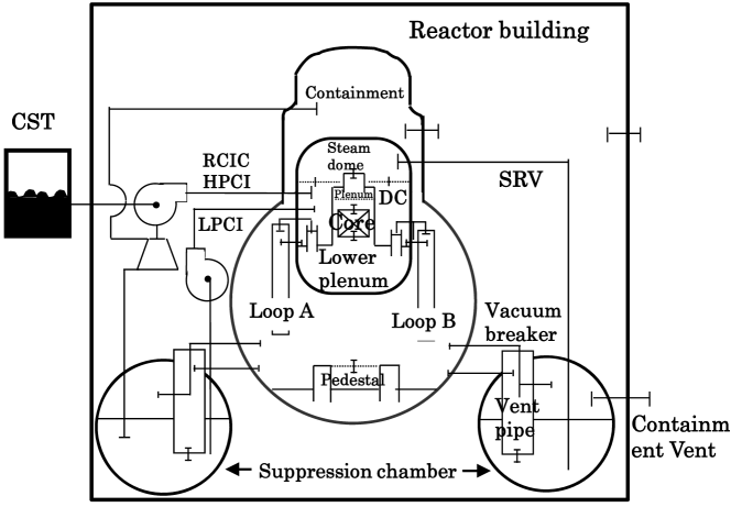
Figure 11: Nodalization of physical space

2pt FP: Fission Products [tl] at 50 -4

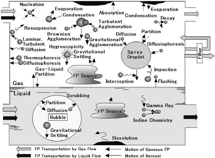
Figure 12: Phenomenon considered for fission product transportation

In this appendix, we present the experimental setting for the Application Study on Nuclear Accident Management in Section 6.4. With THALES2, we consider the volume nodalization as shown in Figure 11. The reactor pressure vessel was divided into seven volumes, consisting of core, upper plenum, lower plenum, steam dome, downcomer, and recirculation loops A and B. The containment vessel consists of drywell, suppression chamber, pedestal and vent pipes. The atmosphere and suppression chamber are connected via the containment venting system (S/C venting). The plant data and initial conditions were determined based on the data of the Unit 1 of the Browns Ferry nuclear power plant (BWR4/Mark-I) and the construction permit application forms of BWR plants in Japan. The failure of the containment vessel is assumed to occur when the pressure of the vessel becomes $2.5$ times greater than the design pressure. Here, the design pressure is $3.92$ (kgf/cm²g) and the criterion for the containment failure is $108330$ kgf/m². The degree of opening for the containment venting was fixed at $25\%$ and no filtering was considered.

We consider the TQUV sequence as the accident scenario. In the TQUV sequence, no Emergency Core Cooling Systems (ECCSs) functions, similar to the case of the accident at the Fukushima Daiichi nuclear power plant. The TQUV sequence is one of the major scenarios considered in Probabilistic Risk Assessment (PRA) of nuclear plants. Therefore, our results show a promising benefit of containment venting, as long as we use it with a good policy.

The simulator we developed at the Japan Atomic Energy Agency and adopted in this experiment (THALES2) computes the transportation of fission products as well as thermal hydraulics in each volume of Figure 11 and core melt progression in the Core volume. The transportation of fission products considered in the experiment is shown in Figure 12. The details of the computation of the THALES2 code are found in the paper by ? (?). Figure 11 and Figure 12 are the modified versions of the graphs used in a previous presentation about the ongoing development of the THALES2 code, which was given at the USNRC’s 25th Regulatory Information Conference (?).

References

- Ansótegui, Sellmann, and Tierney Ansótegui, C., Sellmann, M., and Tierney, K. (2009). A gender-based genetic algorithm for the automatic configuration of algorithms. In Proceedings of the 15th International Conference on Principles and Practice on Constraint Programing (CP 2009).
- Atkeson Atkeson, C. G. (1998). Nonparametric model-based reinforcement learning. In Advances in Neural Information Processing Systems (NIPS), pp. 1008–1014.
- Azar, Lazaric, and Brunskill Azar, M. G., Lazaric, A., and Brunskill, E. (2014). Stochastic optimization of a locally smooth function under correlated bandit feedback. In 31st International Conference on Machine Learning (ICML).
- Baxter and Bartlett Baxter, J., and Bartlett, P. L. (2001). Infinite-horizon policy-gradient estimation. Journal of Artificial Intelligence Research (JAIR), 15, 319–350.
- Birattari, Yuan, Balaprakash, and Stützle Birattari, M., Yuan, Z., Balaprakash, P., and Stützle, T. (2010). F-race and iterated F-race: An overview. In Experimental Methods for the Analysis of Optimization Algorithms, pp. 311–336. Springer-Verlag.
- Brochu, Cora, and de Freitas Brochu, E., Cora, V. M., and de Freitas, N. (2009). A tutorial on Bayesian optimization of expensive cost functions, with application to active user modeling and hierarchical reinforcement learning. Technical report No. UBC TR-2009-23 and arXiv:1012.2599v1, Dept. of Computer Science, University of British Columbia.
- Bubeck and Munos Bubeck, S., and Munos, R. (2010). Open loop optimistic planning. In Conference on Learning Theory.
- Bubeck, Stoltz, and Yu Bubeck, S., Stoltz, G., and Yu, J. Y. (2011). Lipschitz bandits without the Lipschitz constant. In Proceedings of the 22nd International Conference on Algorithmic Learning Theory.
- Busoniu, Daniels, Munos, and Babuska Busoniu, L., Daniels, A., Munos, R., and Babuska, R. (2013). Optimistic planning for continuous-action deterministic systems. In 2013 Symposium on Adaptive Dynamic Programming and Reinforcement Learning.
- Carter, Gablonsky, Patrick, Kelly, and Eslinger Carter, R. G., Gablonsky, J. M., Patrick, A., Kelly, C. T., and Eslinger, O. J. (2001). Algorithms for noisy problems in gas transmission pipeline optimization. Optimization and Engineering, 2(2), 139–157.
- Daly and Shen Daly, R., and Shen, Q. (2009). Learning Bayesian network equivalence classes with ant colony optimization. Journal of Artificial Intelligence Research, 35(1), 391–447.
- Deisenroth, Neumann, and Peters Deisenroth, M. P., Neumann, G., and Peters, J. (2013). A survey on policy search for robotics. Foundations and Trends in Robotics, 2, 1–142.
- Deisenroth and Rasmussen Deisenroth, M. P., and Rasmussen, C. E. (2011). PILCO: A model-based and data-efficient approach to policy search. In 28th International Conference on Machine Learning (ICML).
- Dixon Dixon, L. C. W. (1978). Global Optima Without Convexity. Hatfield, England: Numerical Optimization Centre, Hatfield Polytechnic.
- Gablonsky Gablonsky, J. M. (2001). Modifications of the direct algorithm. Ph.D. thesis, North Carolina State University, Raleigh, North Carolina.
- Gullapalli, Franklin, and Benbrahim Gullapalli, V., Franklin, J., and Benbrahim, H. (1994). Acquiring robot skills via reinforcement learning. Control Systems Magazine, IEEE, 14(1), 13–24.
- Gyorgy and Kocsis Gyorgy, A., and Kocsis, L. (2011). Efficient multi-start strategies for local search algorithms. Journal of Artificial Intelligence Research (JAIR), 41, 407–444.
- Hansen and Jaumard Hansen, P., and Jaumard, B. (1995). Lipschitz optimization. In Horst, R., and Pardalos, P. M. (Eds.), Handbook of Global Optimization, pp. 407–493. The Netherlands: Kluwer Academic Publishers.
- Hansen, Jaumard, and Lu Hansen, P., Jaumard, B., and Lu, S. H. (1991). On the number of iterations of Piyavskii’s global optimization algorithm. Mathematics of Operations Research, 16, 334–350.
- He, Verstak, Sosonkina, and Watson He, J., Verstak, A., Sosonkina, M., and Watson, L. (2009). Performance modeling and analysis of a massively parallel DIRECT, Part 1. Journal of High Performance Computing Applications, 23, 14–28.
- He, Verstak, Watson, Stinson, et al. He, J., Verstak, A., Watson, L. T., Stinson, C. A., et al. (2004). Globally optimal transmitter placement for indoor wireless communication systems. IEEE Transactions on Wireless Communications, 3(6), 1906–1911.
- Heidrich-Meisner and Igel Heidrich-Meisner, V., and Igel, C. (2008). Evolution strategies for direct policy search. In Proceedings of the 10th International Conference on Parallel Problem Solving from Nature: PPSN X, pp. 428–437. Springer-Verlag.
- Horst and Tuy Horst, R., and Tuy, H. (1990). Global Optimization: Deterministic Approaches. Berlin: Springer.
- Hutter, Hoos, and Leyton-Brown Hutter, F., Hoos, H. H., and Leyton-Brown, K. (2011). Sequential model-based optimization for general algorithm configuration. In Learning and Intelligent Optimization, 5, 507–523.
- Hutter, Hoos, Leyton-Brown, and Stützle Hutter, F., Hoos, H. H., Leyton-Brown, K., and Stützle, T. (2009). ParamILS: An automatic algorithm configuration framework. Journal of Artificial Intelligence Research (JAIR), 36, 267–306.
- Ishikawa, Muramatsu, and Sakamoto Ishikawa, J., Muramatsu, K., and Sakamoto, T. (2002). Systematic source term analysis for level 3 PSA of a BWR with Mark-II containment with THALES-2 code. In Proceedings of 10th International Conference of Nuclear Engineering, ICONE-10-22080.
- Jones, Perttunen, and Stuckman Jones, D. R., Perttunen, C. D., and Stuckman, B. E. (1993). Lipschitzian optimization without the Lipschitz constant. Journal of Optimization Theory and Applications, 79(1), 157–181.
- Kawaguchi, Uchiyama, and Muramatsu Kawaguchi, K., Uchiyama, T., and Muramatsu, K. (2012). Efficiency of analytical methodologies in uncertainty analysis of seismic core damage frequency. Journal of Power and Energy Systems, 6(3), 378–393.
- Kawaguchi Kawaguchi, K. (2016a). Bounded optimal exploration in MDP. In Proceedings of the 30th AAAI Conference on Artificial Intelligence (AAAI).
- Kawaguchi Kawaguchi, K. (2016b). Deep learning without poor local minima. Massachusetts Institute of Technology, Technical Report, MIT-CSAIL-TR-2016-005.
- Kawaguchi, Kaelbling, and Lozano-Pérez Kawaguchi, K., Kaelbling, L. P., and Lozano-Pérez, T. (2015). Bayesian optimization with exponential convergence. In Advances in Neural Information Processing (NIPS).
- Kirk Kirk, D. E. (1970). Optimal Control Theory. Englewood Cliffs, NJ: Prentice-Hall.
- Kleinberg, Slivkins, and Upfal Kleinberg, R. D., Slivkins, A., and Upfal, E. (2008). Multi-armed bandit problems in metric spaces. In Proceedings of the 40th ACM Symposium on Theory of Computing, pp. 681–690.
- Kober, Bagnell, and Peters Kober, J., Bagnell, J. A. D., and Peters, J. (2013). Reinforcement learning in robotics: A survey. International Journal of Robotics Research, 32.
- Kvasov, Pizzuti, and Sergeyev Kvasov, D. E., Pizzuti, C., and Sergeyev, Y. D. (2003). Local tuning and partition strategies for diagonal GO methods. Numerische Mathematik, 94(1), 93–106.
- Maruyama Maruyama, Y. (2013). Development of THALES2 code and application to analysis of the accident at Fukushima Daiichi Nuclear Power Plant. In The NRC’s 25th Regulatory Information Conference.
- Mayne and Polak Mayne, D. Q., and Polak, E. (1984). Outer approximation algorithm for nondifferentiable optimization problems. Journal of Optimization Theory and Applications, 42(1), 19–30.
- McDonald, Grantham, Tabor, and Murphy McDonald, D. B., Grantham, W. J., Tabor, W. L., and Murphy, M. J. (2007). Global and local optimization using radial basis function response surface models. Applied Mathematical Modelling, 31(10), 2095–2110.
- Mladineo Mladineo, R. H. (1986). An algorithm for finding the global maximum of a multimodal, multivariate function. Mathematical Programming, 34, 188–200.
- Munos Munos, R. (2011). Optimistic optimization of deterministic functions without the knowledge of its smoothness. In Advances in Neural Information Processing Systems (NIPS), pp. 783–791.
- Munos Munos, R. (2013). From bandits to Monte-Carlo tree search: The optimistic principle applied to optimization and planning. Foundations and Trends in Machine Learning, 7(1), 1–130.
- Murty and Kabadi Murty, K. G., and Kabadi, S. N. (1987). Some np-complete problems in quadratic and nonlinear programming. Mathematical programming, 39(2), 117–129.
- OECD/NEA/CSNI OECD/NEA/CSNI (2014). Status report on filtered containment venting. Technical report NEA/CSNI/R(2014)7, JT03360082.
- Park and Ahn Park, Y., and Ahn, I. (2010). SAMEX: A severe accident management support expert. Annals of Nuclear Energy, 37(8), 1067–1075.
- Pinter Pinter, J. (1986). Globally convergent methods for -dimensional multiextremal optimization. Optimization, 17, 187–202.
- Piyavskii Piyavskii, S. A. (1967). An algorithm for finding the absolute minimum of a function. Theory of Optimal Solutions, 2, 13–24. Kiev, IK AN USSR.
- Rios and Sahinidis Rios, L. M., and Sahinidis, N. V. (2013). Derivative-free optimization: A review of algorithms and comparison of software implementations. Journal of Global Optimization, 56, 1247–1293.
- Russell and Norvig Russell, S. J., and Norvig, P. (2009). Artificial intelligence: A modern approach (3rd edition). Prentice-Hall.
- Ryoo and Sahinidis Ryoo, H. S., and Sahinidis, N. V. (1996). A branch-and-reduce approach to global optimization. Journal of Global Optimization, 8(2), 107–138.
- Shubert Shubert, B. O. (1972). A sequential method seeking the global maximum of a function. SIAM Journal on Numerical Analysis, 9, 379–388.
- Snoek, Larochelle, and Adams Snoek, J., Larochelle, H., and Adams, R. P. (2012). Practical Bayesian optimization of machine learning algorithms. In Advances in Neural Information Processing Systems (NIPS).
- Strongin Strongin, R. G. (1973). On the convergence of an algorithm for finding a global extremum. Engineering Cybernetics, 11, 549–555.
- Surjanovic and Bingham Surjanovic, S., and Bingham, D. (2013). Virtual library of simulation experiments: Test functions and datasets. Retrieved July 2, 2014, from http://www.sfu.ca/~ssurjano.
- Sutton, McAllester, Singh, and Mansour Sutton, R. S., McAllester, D., Singh, S., and Mansour, Y. (1999). Policy gradient methods for reinforcement learning with function approximation. In Advances in Neural Information Processing Systems, 12, 1057–1063.
- USNRC USNRC (2013). Hardened Vents and Filtration for Boiling Water Reactors with Mark I and Mark II containment designs . Retrieved in August 2015 from http://www.nrc.gov/reactors/operating/ops-experience/japan-dashboard/hardened-vents.html .
- Valko, Carpentier, and Munos Valko, M., Carpentier, A., and Munos, R. (2013). Stochastic simultaneous optimistic optimization. In Proceedings of the 30th International Conference on Machine Learning (ICML).
- Wang, Shakibi, Jin, and de Freitas Wang, Z., Shakibi, B., Jin, L., and de Freitas, N. (2014). Bayesian multi-scale optimistic optimization. In AI and Statistics, pp. 1005–1014.
- Wang, Zoghi, Hutter, Matheson, and De Freitas Wang, Z., Zoghi, M., Hutter, F., Matheson, D., and De Freitas, N. (2013). Bayesian optimization in high dimensions via random embeddings. In Proceedings of the Twenty-Third international joint conference on Artificial Intelligence, pp. 1778–1784. AAAI Press.
- Weinstein Weinstein, A. (2014). Local planning for continuous Markov decision processes. Ph.D. thesis, Rutgers, The State University of New Jersey.
- Weinstein and Littman Weinstein, A., and Littman, M. L. (2012). Bandit-based planning and learning in continuous-action Markov decision processes. In International Conference on Automated Planning and Scheduling, pp. 306–314.
- Zheng, Itoh, Kawaguchi, Tamaki, and Maruyama Zheng, X., Itoh, H., Kawaguchi, K., Tamaki, H., and Maruyama, Y. (2015). Application of Bayesian nonparametric models to the uncertainty and sensitivity analysis of source term in a BWR severe accident. Journal of Reliability Engineering & System Safety, 138, 253–262.
- Zwolak, Tyson, and Watson Zwolak, J. W., Tyson, J. J., and Watson, L. T. (2005). Globally optimized parameters for a model of mitotic control in frog egg extracts. IEE Systems Biology, 152(2), 81–92.