Finite-time and finite-size scalings in the evaluation of large-deviation functions:
Analytical study using a birth-death process

Abstract

The Giardinà-Kurchan-Peliti algorithm is a numerical procedure that uses population dynamics in order to calculate large deviation functions associated to the distribution of time-averaged observables. To study the numerical errors of this algorithm, we explicitly devise a stochastic birth-death process that describes the time-evolution of the population-probability. From this formulation, we derive that systematic errors of the algorithm decrease proportionally to the inverse of the population size. Based on this observation, we propose a simple interpolation technique for the better estimation of large deviation functions. The approach we present is detailed explicitly in a two-state model.

I Introduction

Cloning algorithms are numerical procedures aimed at simulating rare events efficiently, using a population dynamics scheme. In such algorithms, copies of the system are evolved in parallel and the ones showing the rare behavior of interest are multiplied iteratively Anderson (1975); Glasserman et al. (1996); Iba (2001); Grassberger (2002); L’Ecuyer et al. (2006); Cappé et al. (2004); van Erp et al. (2003); Allen et al. (2005); Del Moral and Garnier (2005); Dean and Dupuis (2009); Frédéric and Arnaud (2007); Giardinà et al. (2006); Lecomte and Tailleur (2007); Tailleur and Kurchan (2007); Tailleur and Lecomte (2009); Giardinà et al. (2011); Laffargue et al. (2013); Guevara Hidalgo and Lecomte (2016) (See Fig. 1). One of these algorithms proposed by Giardinà et al. Giardinà et al. (2006); Lecomte and Tailleur (2007); Tailleur and Kurchan (2007); Tailleur and Lecomte (2009); Giardinà et al. (2011); Laffargue et al. (2013); Guevara Hidalgo and Lecomte (2016) is used to evaluate numerically the cumulant generating function (a large deviation function, LDF) of additive (or “time-extensive”) observables in Markov processes Dembo and Zeitouni (1998); Touchette (2009). It has been applied to many physical systems, including chaotic systems, glassy dynamics and non-equilibrium lattice gas models, and it has allowed the study of novel properties, such as the behavior of breathers in the Fermi-Pasta-Ulam-Tsingou chain Tailleur and Kurchan (2007), dynamical phase transitions in kinetically constrained models Garrahan et al. (2007), and an additivity principle for simple exclusion processes Bodineau and Derrida (2004); Hurtado and Garrido (2010).

While the method has been used widely, there have been fewer studies focusing on the analytical justification of the algorithm. Even though it is heuristically believed that the LDF estimator converges to the correct result as the number of copies $N_{c}$ increases, there is no proof of this convergence. Related to this lack of the proof, although we use the algorithm by assuming its validity, we do not have any clue how fast the estimator converges as $N_{c}\rightarrow\infty$. In order to discuss this convergence, we define two types of numerical errors. First, for a fixed finite $N_{c}$, averaging over a large number of realizations, the LDF estimator converges to an incorrect value, which is different from the desired large deviation result. We call this deviation from the correct value, systematic errors. Compared with these errors, we also consider the fluctuations of the estimated value. More precisely, for a fixed value of $N_{c}$, the results obtained in different realizations are distributed around this incorrect value. We call the errors associated to these fluctuations the stochastic errors. Although both errors are important in numerical simulations, the former one can lead this algorithm to produce wrong results. For example as seen in Ref. Nemoto et al. (2016), the systematic error grows exponentially as a temperature decreases (or generically in the weak noise limit of diffusive dynamics).

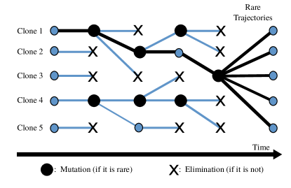
Figure 1: Schematic picture illustrating the principle of the population dynamics algorithm. ‘Clones’ (or copies) of the system are prepared and they evolve following a mutation-and-selection process, maintaining the total population constant.

In order to study these errors, we employ a birth-death process Kampen (2007); Gardiner (1983) description of the population dynamics algorithm as explained below: We focus on physical systems described by a Markov dynamics Giardinà et al. (2006, 2011); Lecomte and Tailleur (2007) with a finite number of states $M$, and we denote by $i$ ($i=0,1,\cdots M-1$) the states of the system. This Markov process has its own stochastic dynamics, described by the transition rates $w(i\rightarrow j)$. In population dynamics algorithms, in order to study its rare trajectories, one prepares $N_{c}$ copies of the system, and simulate these copies according to (i) the dynamics of $w(i\rightarrow j)$ (followed independently by all copies) and (ii) ‘cloning’ step in which the ensemble of copies is directly manipulated, i.e., some copies are eliminated while some are multiplied (See Table 1). Formally, the population dynamics represents, for a single copy of the system, a process that does not preserve probability. This fact has motivated the studies of auxiliary processes Jack and Sollich (2010), effective processes Popkov et al. (2010) and driven processes Chetrite and Touchette (2013) to construct modified dynamics (and their approximations Nemoto and Sasa (2014)) that preserve probability. Different from these methods, in this article, we formulate explicitly the meta-dynamics of the copies themselves by using a stochastic birth-death process. The process preserves probability, and it allows us to study the numerical errors of the algorithm when evaluating LDF.

Table 1: Correspondence between the population dynamics and the birth-death process to describe it.

	Population dynamics algorithm	Birth-death process describing
		the population dynamics
| State of the system	$i$	$n=(n_{0},n_{2},\cdots,n_{M-1})$
	($i=0,1,\cdots M-1$)	($0\leq n_{i}\leq N_{c}$ with $\sum_{i}n_{i}=N_{c}$)
| Transition rates	$w(i\rightarrow j)$	$\sigma(n\rightarrow\tilde{n})$
	Markov process on states $i$	Markov process on states $n$
| Numerical procedure	Prepare $N_{c}$ clones and evolve those	Described by the dynamics
for rare-event sampling	with a mutation-selection procedure	of rates $\sigma(n\rightarrow\tilde{n})$

In this article, we consider the dynamics of the copies as a stochastic birth-death process whose state is denoted $n=(n_{0},n_{1},n_{2},\cdots,n_{M-1})$, where $0\leq n_{i}\leq N_{c}$ represents the number of copies which are in state $i$ in the ensemble of copies. We explicitly introduce the transition rates describing the dynamics of $n$, which we denote by $\sigma(n\rightarrow\tilde{n})$. We show that the dynamics described by these transition rates lead in general to the correct LDF estimation of the original system $w(i\rightarrow j)$ in the $N_{c}\rightarrow\infty$ limit. We also show that the systematic errors are of the order $\mathcal{O}(1/N_{c})$, whereas the numerical errors are of the order $\mathcal{O}(1/(\tau N_{c}))$ (where $\tau$ is an averaging duration). This result is in clear contrast with standard Monte-Carlo methods, where the systematic errors are always 0. Based on this convergence speed, we then propose a simple interpolation technique to make the cloning algorithm more reliable. Furthermore, the formulation developed in this paper provides us the possibility to compute exactly the expressions of the convergence coefficients, as we do in Sec. IV on a simple example.

The analytical analysis presented in this paper is supplemented with a thorough numerical study in a companion paper Guevara Hidalgo et al. (2016). In the companion paper, we employ an intrinsically different cloning algorithm, which is the continuous-time population dynamics algorithm, that cannot be studied by the methods presented in this paper (see Sec. II.4.2). We show in the companion paper Guevara Hidalgo et al. (2016) that the validity of the scaling that we derive analytically here is very general. In particular, we demonstrate in practice the efficiency of the interpolation technique in the evaluation of the LDF, irrespective of the details of the population dynamics algorithm.

The construction of this paper is as follows. We first define the LDF problem in the beginning of Sec. II, and then formulate the birth-death process used to describe the algorithm in Sec. II.1. By using this birth-death process, we demonstrate that the estimator of the algorithm converges to the correct large deviation function in Sec. II.2. At the end of this section, in Sec. II.3, we discuss the convergence speed of this estimator (the systematic errors) and derive its scaling $\sim 1/N_{c}$. In Sec. III, we turn to stochastic errors. For discussing this, we introduce the large deviation function of the estimator, from which we derive that the convergence speed of the stochastic errors is proportional to $1/(\tau N_{c})$. In the next section, Sec. IV, we introduce a simple two-state model, to which we apply the formulations developed in the previous sections. We derive the exact expressions of the systematic errors in Sec. IV.1 and of the stochastic errors in Sec. IV.2. At the end of this section, in Sec. IV.3, based on these exact expressions, we propose another large deviation estimator defined in the population dynamics algorithm. In the final section, Sec. V, we first summarize the result obtained throughout this paper, and then in Sec. V.1, we propose a simple interpolation technique based on the convergence speed of the systematic errors which allows us to devise a better practical evaluation of the LDF. Finally in Sec. V.2, we discuss two open questions.

II Birth-Death Process Describing the Population Dynamics Algorithm

As explained in the introduction (also see Table 1), the state of the population is $n=(n_{0},n_{1},\cdots,n_{M-1})$, where $n_{i}$ represents the number of clones in the state $i$. The total population is preserved: $\sum_{i}n_{i}=N_{c}$. Below, we introduce the transition rates of the dynamics between the occupations $n$, $\sigma(n\rightarrow\tilde{n})$ that describe corresponding large deviations of the original system, where the dynamics of the original system is given by the rates $w(i\rightarrow j)$ as detailed below.

As the original system, we consider the continuous-time Markov process in a discrete-time representation. By denoting by $dt$ the time step, the transition matrix $R_{j,i}$ for time evolution of the state $i$ is described as

$$R_{j,i}=\delta_{i,j}+dt\Big{[}w(i\rightarrow j)-\delta_{i,j}\sum_{k}w(i\rightarrow k)\Big{]},$$ (1)

where we set $w(i\rightarrow i)=0$. The probability distribution of the state $i$, $p_{i}(t)$, evolves in time as $p_{i}(t+dt)=\sum_{j}R_{i,j}p_{j}(t)$. In the $dt\rightarrow 0$ limit, one obtains the continuous-time master equation describing the evolution of $p_{i}(t)$ Kampen (2007); Gardiner (1983). For simplicity, especially for the cloning part of the algorithm, we keep here a small finite $dt$. The reason why we use a discrete-time representation is solely for simplicity of the discussion. The main results can be derived even if we start with a continuous-time representation (see Sec. II.4.1). For the original dynamics described by the transition matrix (1), we consider an observable $b_{i}$ depending on the state $i$ and we are interested in the distribution of its time-averaged value during a time interval $\tau$, defined as

$$B(\tau)=\frac{1}{\tau}\sum_{t=0}^{\tau/dt}dt\ b_{i(t)}.$$ (2)

Here $i(t)$ is a trajectory of the system generated by the Markov dynamics described by $R_{j,i}$. We note that $B(\tau)$ is a path- (or history-, or realization-) dependent quantity. Since $\tau B(\tau)$ is an additive observable, the fluctuations of $B(\tau)$ depending on the realizations are small when $\tau$ is large, but one can describe the large deviations of $B(\tau)$. Those occur with a small probability, and obey a large deviation principle. We denote by ${\rm Prob}(B)$ the distribution function of $B(\tau)$. The large deviation principle ensures that ${\rm Prob}(B)$ takes an asymptotic form ${\rm Prob}(B)\sim\exp(-\tau I(B))$ for large $\tau$, where $I(B)$ is a large deviation function (or ‘rate function’) Touchette (2009); Dembo and Zeitouni (1998). If the rate function $I(B)$ is convex, the large deviation function is expressed as a Legendre transform of a cumulant generating function (CGF) $\psi(s)$ defined as

$$\psi(s)=\lim_{\tau\rightarrow\infty}\frac{1}{\tau}\log\left\langle e^{-s\tau B(\tau)}\right\rangle,$$ (3)

namely: $I(B)=-\inf_{s}\left[sB+\psi(s)\right]$. The large deviation function $I(B)$ and this generating function $\psi(s)$ are by definition difficult to evaluate numerically in Monte-Carlo simulations of the original system of transition rates $w(i\rightarrow j)$ (see, for example, Rohwer et al. (2015)). To overcome this difficulty, population dynamics algorithms have been developed Giardinà et al. (2006); Lecomte and Tailleur (2007); Tailleur and Kurchan (2007); Tailleur and Lecomte (2009); Giardinà et al. (2011); Laffargue et al. (2013); Guevara Hidalgo and Lecomte (2016). Here, we describe this population dynamics algorithm by using a birth-death process on the occupation state $n$ allowing us to study systematically the errors in the estimation of $\psi(s)$ within the population dynamics algorithm. We mention that, without loss of generality, we restrict our study to so-called ‘type-B’ observables that do not depend on the transitions of the state Garrahan et al. (2009), i.e. which are time integrals of the state of the system, as in (2). Indeed, as explained for example in Refs. Giardinà et al. (2011) and Nemoto et al. (2016), one can always reformulate the determination of the CGF of mixed-type observables into that of a type-B variable, by modifying the transition rates of the given system.

II.1 Transition Matrices Representing the Population Dynamics Algorithm

We denote the probability distribution of the occupation $n$ at time $t$ by $P_{n}(t)$. The time-evolution of this probability is decomposed into three parts. The first one is the original Monte-Carlo dynamics based on the transition rates $w(i\rightarrow j)$. The second one is the cloning procedure of the population dynamics algorithm, which favors or disfavors configurations according to a well-defined rule. The third one is a supplementary (but important) part which maintains the total number of clones to a constant $N_{c}$. We denote the transition matrices corresponding to these steps by $\mathcal{T}$, $\mathcal{C}$ and $\mathcal{K}$, respectively. By using these matrices, then, the time evolution of the distribution function is given as

$$P_{n}(t+dt)=\sum_{\tilde{n}}\left(\mathcal{K}\mathcal{C}\mathcal{T}\right)_{n,\tilde{n}}P_{\tilde{n}}(t).$$ (4)

We derive explicit expressions of these matrices in the following sub-sections. We also summarize the obtained results in Table 2.

Table 2: Transition matrices (see Eq. (4)) describing the birth-death process.

	Transition matrices
| Dynamics (“mutations”)	$\mathcal{T}_{\tilde{n},n}\equiv\delta_{\tilde{n},n}+dt\sum_{i=0}^{M-1}n_{i}\sum_{j=0,(j\neq i)}^{M-1}w(i\rightarrow j)\left[\delta_{\tilde{n}_{i},n_{i}-1}\delta_{\tilde{n}_{j},n_{j}+1}\ \delta^{i,j}_{\tilde{n},n}\ -\delta_{\tilde{n},n}\right]$
| Cloning (“selection”)	$\mathcal{C}_{\tilde{n},n}=\delta_{\tilde{n},n}+s\ dt\sum_{i=0}^{M-1}n_{i}|\alpha_{i}|\left[\delta_{\tilde{n}_{i},n_{i}+\alpha_{i}/|\alpha_{i}|}\ \delta^{i}_{\tilde{n},n}-\delta_{\tilde{n},n}\right]+\mathcal{O}(dt^{2})$
| Maintaining $N_{c}$	$\mathcal{K}_{\tilde{n},n}=\delta_{\sum n_{i},N_{c}}\delta_{\tilde{n},n}+\sum_{k=-1,1}\delta_{\sum_{i}n_{i},N_{c}+k}\sum_{i=0}^{M-1}\delta_{\tilde{n}_{i},n_{i}-k}\ \delta^{i}_{\tilde{n},n}\ \frac{n_{i}}{N_{c}+k}$
| Full process	$(\mathcal{K}\mathcal{C}\mathcal{T})_{\tilde{n},n}=\delta_{\tilde{n},n}+dt\sum_{i=0}^{M-1}n_{i}\sum_{j=0,(j\neq i)}^{M-1}\left[w(i\rightarrow j)+s\tilde{w}_{n}(i\rightarrow j)\right]\left[\delta_{\tilde{n}_{i},n_{i}-1}\delta_{\tilde{n}_{j},n_{j}+1}\ \delta^{i,j}_{\tilde{n},n}\ -\delta_{\tilde{n},n}\right]$
	with     $\tilde{w}_{n}(i\rightarrow j)=\frac{n_{j}}{N_{c}}\left[\alpha_{j}\delta_{j\in\Omega^{(+)}}\frac{N_{c}}{N_{c}+1}-\alpha_{i}\delta_{i\in\Omega^{(-)}}\frac{N_{c}}{N_{c}-1}\right]$

II.1.1 Derivation of the Original Dynamics Part, $\mathcal{T}$

We first consider the transition matrix $\mathcal{T}$, which describes the evolution of the occupation state $n$ solely due to the dynamics based on the rates $w(i\rightarrow j)$. During an infinitesimally small time step $dt$, the occupation $n=(n_{0},n_{1},\cdots,n_{M-1})$ changes to $\tilde{n}=(n_{0},n_{1},\cdots,n_{i}-1,\cdots,n_{j}+1,\cdots,n_{M-1})$ where $0\leq i<M$ and $0\leq j<M$ (for all $i\neq j$). Since there are $n_{i}$ clones in the state $i$ before the transition, the transition probability of this change is given as $n_{i}w(i\rightarrow j)dt$. Thus, we obtain

$$\begin{split}\mathcal{T}_{\tilde{n},n}\equiv\delta_{\tilde{n},n}+&dt\sum_{i=0}^{M-1}n_{i}\sum_{j=0,(j\neq i)}^{M-1}w(i\rightarrow j)\\ &\times\left[\delta_{\tilde{n}_{i},n_{i}-1}\delta_{\tilde{n}_{j},n_{j}+1}\ \delta^{i,j}_{\tilde{n},n}\ -\delta_{\tilde{n},n}\right],\end{split}$$ (5)

where $\delta^{i,j}_{\tilde{n},n}$ is a Kronecker-delta for the indices except for $i,j$: $\delta^{i,j}_{\tilde{n},n}\equiv\prod_{k\neq i,j}\delta_{\tilde{n}_{k},n_{k}}$. One can easily check that this matrix satisfies the conservation of the probability: $\sum_{\tilde{n}}\mathcal{T}_{\tilde{n},n}=1$. It corresponds to the evolution of $N_{c}$ independent copies of the original system with rates $w(i\to j)$.

II.1.2 Derivation of the Cloning Part, $\mathcal{C}$

In the population dynamics algorithm (for example the one described in the Appendix A of Ref. Nemoto et al. (2016)), at every certain time interval $\Delta t$, one evaluates the exponential factor for all clones, which is equal to $e^{-s\int_{t}^{t+\Delta t}\!dt^{\prime}~{}b_{i(t^{\prime})}}$ if the clone is in state $(i(t^{\prime}))_{t^{\prime}=t}^{t+\Delta t}$ during a time interval $t\leq t^{\prime}\leq t+\Delta t$. We also call this exponential factor cloning ratio, because this factor determines whether each clone is copied or eliminated after this time interval. Although the details of how to determine this selection process can depend on the specific type of algorithms, the common idea is that each of the clones is copied or eliminated in such a way that a clone in state $i(t)$ has a number of descendant(s) proportional to the cloning factor on average after this time interval.

In order to implement this idea in our birth-death process, we assume this time step $\Delta t$ to be small. For the sake of simplicity, we set this $\Delta t$ to be our smallest time interval $dt$: $\Delta t=dt$. This condition is not mandatory whenever the $\Delta t\rightarrow 0$ limit is taken at the end (see Sec. II.4.1 for the case $\Delta t>dt$). Then, noticing that the time integral $\int_{t}^{t+\Delta t}dt^{\prime}~{}b_{i(t^{\prime})}$ is expressed as $dt\ b_{i(t)}$ for small $dt$, we introduce the following quantity for each state $i$ ($i=0,1,2,...,M-1$):

$$\nu_{i}\equiv\frac{n_{i}e^{-s~{}dt~{}b_{i}}}{\sum_{j=0}^{M-1}n_{j}e^{-s~{}dt~{}b_{j}}}N_{c}.$$ (6)

Note that there is a factor $n_{i}$ in front of the exponential function $e^{-s~{}dt~{}b_{i}}$ which enumerates the number of clones that occupy the state $i$. The quantity $\nu_{i}$ is aimed at being the number of clones in state $i$ after the cloning process, however, since $\nu_{i}$ is not an integer but a real number, one needs a supplementary prescription to fix the corresponding integer number of descendants. In general, in the implementation of population dynamics, this integer is generated randomly from the factor $\nu_{i}$, equal either to its lower or to its upper integer part. The probability to choose either the lower or upper integer part is fixed by imposing that the number of descendants is equal to $\nu_{i}$ on average. For instance, if $\nu_{i}$ is equal to $13.2$, then $13$ is chosen with probability $0.8$, and $14$ with probability $0.2$. Generically, $\lfloor\nu_{i}\rfloor$ and $\lfloor\nu_{i}\rfloor+1$ are chosen with probability $1+\lfloor\nu_{i}\rfloor-\nu_{i}$ and $\nu_{i}-\lfloor\nu_{i}\rfloor$, respectively. We note that we need to consider these two possibilities for all indices $i$. We thus arrive at the following matrix:

$$\begin{split}\mathcal{C}_{\tilde{n},n}\equiv&\sum_{x_{0}=0}^{1}\sum_{x_{1}=0}^{1}\sum_{x_{2}=0}^{1}\cdots\sum_{x_{M-1}=0}^{1}\prod_{i=0}^{M-1}\\ &\times\delta_{\tilde{n}_{i},\lfloor\nu_{i}\rfloor+x_{i}}\left[\left(\nu_{i}-\lfloor\nu_{i}\rfloor\right)x_{i}+\left(1+\lfloor\nu_{i}\rfloor-\nu_{i}\right)(1-x_{i})\right].\end{split}$$ (7)

Now, we expand $\mathcal{C}$ at small $dt$ and we keep only the terms proportional to $\mathcal{O}(1)$ and $\mathcal{O}(dt)$, which do not vanish in the continuous-time limit. For this purpose, we expand $\nu_{i}$ as

$$\nu_{i}=n_{i}\bigg{[}1+s\ dt\Big{(}\sum_{j}\frac{n_{j}b_{j}}{N_{c}}-b_{i}\Big{)}\bigg{]}+\mathcal{O}(dt^{2}),$$ (8)

where we have used $\sum_{i}n_{i}=N_{c}$. This expression indicates that $\lfloor\nu_{i}\rfloor$ is determined depending on the sign of $\sum_{j}n_{j}b_{j}/N_{c}-b_{i}$, where we assumed $s>0$ for simplicity without loss of generality (because when $s<0$, we can always re-define $-b$ as $b$ to make $s$ to be positive). By denoting this factor by $\alpha_{i}$, i.e.

$$\alpha_{i}(n)\equiv\sum_{j}\frac{n_{j}b_{j}}{N_{c}}-b_{i},$$ (9)

we thus define the following state-space $\Omega^{(\pm)}(n)$:

$$\Omega^{(\pm)}(n)=\left\{\ i\ \big{|}\ 0\leq i<M\ {\rm and}\ \pm\alpha_{i}(n)>0\right\}.$$ (10)

From this definition, for sufficiently small $dt$, we obtain

$$\left\lfloor\nu_{i}\right\rfloor=n_{i}$$ (11)

for $i\in\Omega^{(+)}$, and

$$\left\lfloor\nu_{i}\right\rfloor=n_{i}-1$$ (12)

for $i\in\Omega^{(-)}$. Substituting these results into (7) and expanding in $dt$, we obtain (denoting here and thereafter $\alpha_{i}=\alpha_{i}(n))$:

$$\begin{split}\mathcal{C}_{\tilde{n},n}=&\delta_{\tilde{n},n}+s\ dt\sum_{i=0}^{M-1}n_{i}|\alpha_{i}|\big{[}\delta_{\tilde{n}_{i},n_{i}+\alpha_{i}/|\alpha_{i}|}\ \delta^{i}_{\tilde{n},n}-\delta_{\tilde{n},n}\big{]}\\ &+\mathcal{O}(dt^{2}),\end{split}$$ (13)

where $\delta^{i}_{\tilde{n},n}$ is a Kronecker delta for the indices except for $i$: $\delta^{i}_{\tilde{n},n}=\prod_{k\neq i}\delta_{\tilde{n}_{k},n_{k}}$. One can easily check that this matrix preserves probability: $\sum_{\tilde{n}}\mathcal{C}_{\tilde{n},n}=1$.

II.1.3 Derivation of the Maintaining Part, $\mathcal{K}$

As directly checked, the operator $\mathcal{T}$ preserves the total population $\sum_{i}n_{i}$. However, the operator representing the cloning $\mathcal{C}$, does not. In our birth-death implementation, this property originates from the rounding process $\lfloor\nu_{i}\rfloor$ in the definition of $\mathcal{C}$: even though $\nu_{i}$ itself satisfies $\sum_{i}\nu_{i}=N_{c}$, because of the rounding process of $\nu_{i}$, the number of clones after multiplying by $\mathcal{C}$ (that is designed to be proportional to $\nu_{i}$ on average) can change. There are several ways to keep the number $N_{c}$ of copies constant without biasing the distribution of visited configurations. One of them is to choose randomly and uniformly $\delta N_{c}$ clones from the ensemble, where $\delta N_{c}$ is equal to the number of excess (resp. lacking) clones with respect to $N_{c}$, and to eliminate (resp. multiply) them.

In our birth-death description, we implement this procedure as follows. We denote by $\mathcal{K}$ the transition matrix maintaining the total number of clones to be the constant $N_{c}$. We now use a continuous-time asymptotics $dt\rightarrow 0$. In this limit, from the expression of the transition matrix elements (13), we find that at each cloning step the number of copies of the cloned configuration varies by $\pm 1$ at most. Hence, the total number of clones after multiplying by $\mathcal{C}$, $\sum_{i}n_{i}$, satisfies the following inequality

$$N_{c}-1\leq\sum_{i}n_{i}\leq N_{c}+1.$$ (14)

Among the configurations $n$ that satisfy this inequality, there are three possibilities, which are $\sum_{i}n_{i}=N_{c}$ and $\sum_{i}n_{i}=N_{c}\pm 1$. If $n$ satisfies $\sum_{i}n_{i}=N_{c}$, we do not need to adjust $n$, while if $n$ satisfies $\sum_{i}n_{i}=N_{c}+1$ (resp. $\sum_{i}n_{i}=N_{c}-1$), we eliminate (resp. multiply) a clone chosen randomly and uniformly. Note that, in our formulation, we do not distinguish the clones taking the same state. This means that we can choose one of the occupations $n_{i}$ of a state $i$ according to a probability proportional to the number of copies $n_{i}$ in this state. In other words, the probability to choose the state $i$ and to copy or to eliminate a clone from this state is proportional to $n_{i}/\sum_{j=0}^{M-1}n_{j}$. Therefore, we obtain the expression of the matrix $\mathcal{K}$ as

$$\begin{split}\mathcal{K}_{\tilde{n},n}=&\delta_{\sum_{i}\!n_{i},N_{c}}\delta_{\tilde{n},n}\\ &+\sum_{k=-1,1}\delta_{\sum_{i}\!n_{i},N_{c}+k}\sum_{i=0}^{M-1}\delta_{\tilde{n}_{i},n_{i}-k}\ \delta^{i}_{\tilde{n},n}\ \frac{n_{i}}{N_{c}+k}\end{split}$$ (15)

for $\tilde{n}$ that satisfies $\sum_{i}\tilde{n}_{i}=N_{c}$, and $\mathcal{K}_{\tilde{n},n}=0$ otherwise.

II.1.4 Total Transition, $\mathcal{K}\mathcal{C}\mathcal{T}$

We write down the matrix describing the total transition of the population dynamics (see Eq. (4)). From the obtained expressions of $\mathcal{K}$, $\mathcal{C}$, $\mathcal{T}$, we calculate $\mathcal{K}\mathcal{C}\mathcal{T}$

$$\begin{split}&(\mathcal{K}\mathcal{C}\mathcal{T})_{\tilde{n},n}=\delta_{\tilde{n},n}\\ &+dt\sum_{i=0}^{M-1}n_{i}\sum_{j=0,(j\neq i)}^{M-1}\left[w(i\rightarrow j)+s\,\tilde{w}_{n}(i\rightarrow j)\right]\\ &\qquad\qquad\times\left[\delta_{\tilde{n}_{i},n_{i}-1}\delta_{\tilde{n}_{j},n_{j}+1}\ \delta^{i,j}_{\tilde{n},n}\ -\delta_{\tilde{n},n}\right],\end{split}$$ (16)

where the population-dependent transition rate $\tilde{w}_{n}(i\rightarrow j)$ is given as

$$\tilde{w}_{n}(i\rightarrow j)=\frac{n_{j}}{N_{c}}\left[\alpha_{j}\delta_{j\in\Omega^{(+)}}\frac{N_{c}}{N_{c}+1}-\alpha_{i}\delta_{i\in\Omega^{(-)}}\frac{N_{c}}{N_{c}-1}\right].$$ (17)

The comparison of the expression (16) with the original part $\mathcal{T}$ provides an insight into the obtained result. The jump ratio $w(i\rightarrow j)$ in the original dynamics is replaced by $w(i\rightarrow j)+s\,\tilde{w}_{n}(i\rightarrow j)$ in the population dynamics algorithm. We note that this transition rate depends on the population $n$, meaning that we cannot get a closed equation for this modified dynamics at the level of the states $i$ in general. We finally remark that the transition matrix $\sigma(n\rightarrow\tilde{n})$ for the continuous-time limit is directly derived from (16) as

$$\begin{split}&\sigma(n\rightarrow\tilde{n})=\sum_{i=0}^{M-1}n_{i}\sum_{j=0,(j\neq i)}^{M-1}\left[w(i\rightarrow j)+s\tilde{w}_{n}(i\rightarrow j)\right]\\ &\qquad\qquad\qquad\times\left[\delta_{\tilde{n}_{i},n_{i}-1}\delta_{\tilde{n}_{j},n_{j}+1}\ \delta^{i,j}_{\tilde{n},n}\right].\end{split}$$ (18)

II.2 Derivation of the Large Deviation Results
in the $N_{c}\rightarrow\infty$ Asymptotics

In this subsection, we study the $N_{c}\rightarrow\infty$ limit for the transition matrix of rates $\sigma(n\rightarrow\tilde{n})$, and derive the validity of the population dynamics algorithm.

II.2.1 The Estimator of the Large Deviation Function

One of the ideal implementations of the population dynamics algorithm is as follows: We make copies of each realization (clone) at the end of simulation, where the number of copies for each realization is equal to the exponential weight $e^{-s\tau B(\tau)}$ in Eq. (3) (so that we can discuss an ensemble with this exponential weight without multiplying the probability by it). In this implementation, the number of clones grows (or decays) exponentially proportionally as $\left\langle e^{-s\tau B(\tau)}\right\rangle$ by definition. In real implementations of the algorithm, however, since taking care of an exponentially large or small number of clones can cause numerical problems, one rather keeps the total number of clones to a constant $N_{c}$ at every time step, as seen in (6). Within this implementation, we reconstruct the exponential change of the total number of clones as follows: We compute the average of cloning ratio (see the beginning of Sec. II.1.2 for its definition) at each cloning step, and we store the product of these ratios along the cloning steps. At final time, this product gives the empirical estimation of total (unnormalized) population during the whole duration of the simulation Guevara Hidalgo and Lecomte (2016), i.e. an estimator of $\left\langle e^{-s\tau B(\tau)}\right\rangle$. One thus estimates the CGF $\psi(s)$ given in Eq. (3) Giardinà et al. (2006); Lecomte and Tailleur (2007); Tailleur and Kurchan (2007); Tailleur and Lecomte (2009); Giardinà et al. (2011); Laffargue et al. (2013); Guevara Hidalgo and Lecomte (2016) as the logarithm of this reconstructed population, divided by the total time.

In our formulation, the average cloning ratio is given as $\sum_{i}n_{i}e^{-sdtb_{i}}/N_{c}$, and thus the multiplication over whole time interval reads $\prod_{t=0}^{\tau/dt}\{n_{i}(t)e^{-sdtb_{i}}/N_{c}\}$. Because we empirically assume that the CGF estimator converges to $\psi(s)$ in the $N_{c},\tau\rightarrow\infty$ limit, the following equality is expected to hold in probability 1:

$$\psi(s)\stackrel{{\scriptstyle?}}{{=}}\lim_{N_{c}\rightarrow\infty}\lim_{\tau\rightarrow\infty}\frac{1}{\tau}\sum_{t=0}^{\tau/dt}\ \log\sum_{i}\frac{n_{i}(t)e^{-sdtb_{i}}}{N_{c}}+O(dt).$$ (19)

Since the dynamics of the population $n$ is described by a Markov process, ergodicity is satisfied, i.e., time averages can be replaced by the expected value with respect to the stationary distribution function. Applying this result to the right-hand side of (19), we obtain

$$\begin{split}&\lim_{\tau\rightarrow\infty}\frac{1}{\tau}\sum_{t=0}^{\tau/dt}\ \log\sum_{i}\frac{n_{i}(t)e^{-sdtb_{i}}}{N_{c}}\\ &=\frac{1}{dt}\sum_{n}P_{n}^{\rm st}\ \log\sum_{i}\frac{n_{i}e^{-sdtb_{i}}}{N_{c}}+\mathcal{O}(dt),\end{split}$$ (20)

where $P_{n}^{\rm st}$ is the stationary distribution function of the population $n$ in the $dt\rightarrow 0$ limit, (namely, $P_{n}^{\rm st}$ is the stationary distribution of the dynamics of transition rates $\sigma(n\rightarrow\tilde{n})$). By expanding this right-hand side with respect to $dt$, we rewrite the expected equality (19) as

$$\psi(s)\stackrel{{\scriptstyle?}}{{=}}-s\lim_{N_{c}\rightarrow\infty}\sum_{n}P_{n}^{\rm st}\sum_{i}\frac{n_{i}b_{i}}{N_{c}}+O(dt).$$ (21)

where we used that $\sum_{i}n_{i}=N_{c}$ is a conserved quantity. Below we demonstrate that this latter equality (21) is satisfied by analyzing the stationary distribution function $P_{n}^{\rm st}$.

II.2.2 The Connection between the Distribution Functions
of the Population and of the Original System

From the definition of the stationary distribution function $P_{n}^{\rm st}$, we have

$$\sum_{\tilde{n}}P_{\tilde{n}}^{\rm st}\sigma(\tilde{n}\rightarrow n)-\sum_{\tilde{n}}P_{n}^{\rm st}\sigma(n\rightarrow\tilde{n})=0,$$ (22)

(which is a stationary Master equation.) In this equation, we use the explicit expression of $\sigma$ shown in (18). By denoting by $n^{j\rightarrow i}$ the configuration where one clone in the state $j$ moves to the state $i$: $n^{j\rightarrow i}\equiv(n_{0},n_{1},\cdots,n_{i}+1,\cdots,n_{j}-1,\cdots,n_{M-1})$, and the stationary master equation (22) is rewritten as

$$\sum_{i,j(i\neq j)}\left[f_{i\rightarrow j}(n^{j\rightarrow i})-f_{i\rightarrow j}(n)\right]=0,$$ (23)

where we defined $f_{i\rightarrow j}(n)$ as

$$f_{i\rightarrow j}(n)=P_{n}^{\rm st}n_{i}\left[w(i\rightarrow j)+s\tilde{w}_{n}(i\rightarrow j)\right].$$ (24)

Now we multiply expression (23) by $n_{k}$ ($k$ is arbitrary from $k=0,1,2,\cdots,M-1$), and sum it over all configurations $n$:

$$\sum_{n}\sum_{i,j(i\neq j)}n_{k}\left[f_{i\rightarrow j}(n^{j\rightarrow i})-f_{i\rightarrow j}(n)\right]=0.$$ (25)

We can change the dummy summation variable $n$ in the first term to $n^{i\rightarrow j}$, which leads to $\sum_{n}\sum_{i,j(i\neq j)}(n^{i\rightarrow j})_{k}f_{i\rightarrow j}(n)$. Since the second term has almost the same expression as the first one except for the factor $n_{k}$, the sum in (25) over the indices $(i,j)$, where none of $i$ nor $j$ is equal to $k$, becomes 0. The remaining term in (25) is thus

$$\begin{split}0&=\sum_{n}\sum_{j(j\neq k)}\left((n^{k\rightarrow j})_{k}-n_{k}\right)f_{k\rightarrow j}(n)\\ &+\sum_{n}\sum_{i(i\neq k)}\left((n^{i\rightarrow k})_{k}-n_{k}\right)f_{i\rightarrow k}(n).\end{split}$$ (26)

Using the definition of $n^{i\rightarrow j}$ in this equation, we arrive at

$$0=\sum_{n}\bigg{[}\sum_{i(i\neq k)}f_{i\rightarrow k}(n)-f_{k\rightarrow i}(n)\bigg{]}.$$ (27)

This equation (27) connects the stationary property of the population dynamics (described by the occupation states $n$) and the one in the original system (described by the states $i$).

The easiest case where we can see this connection is when $s=0$. By defining the empirical occupation probability of the original system as $p_{i}\equiv\sum_{n}P_{n}^{\rm st}n_{i}/N_{c}$, Eq. (27) leads to the following (stationary) master equation for $w(i\rightarrow j)$:

$$0=\sum_{j}p_{j}w(j\rightarrow i)-\sum_{j}p_{i}w(i\rightarrow j)\quad\textnormal{(for $s=0$)}$$ (28)

This is valid for any $N_{c}$, meaning that, for original Monte-Carlo simulations in $s=0$, the empirical probability $p_{i}$ is exactly equal to the steady-state probability, as being the unique solution of (28). It means that there are no systematic errors in the evaluation of $p_{i}$ (see the introduction of this paper for the definition of the term “systematic errors”). However, in the generic case $s\neq 0$, this property is not satisfied. One thus needs to understand the $N_{c}\rightarrow\infty$ limit to connect the population dynamics result with the large deviation property of the original system.

II.2.3 Justification of the Convergence of the Large Deviation Estimator as Population Size becomes Large

In order to take the $N_{c}\rightarrow\infty$ limit, we define a scaled variable $x_{i}$ as $n_{i}/N_{c}$. With keeping this occupation fractions $x_{i}$ to be $\mathcal{O}(1)$, we take the $N_{c}\rightarrow\infty$ limit in (27), which leads to

$$\begin{split}0=\sum_{n}P_{n}^{\rm st}&\Bigg{[}\sum_{j}x_{j}w(j\rightarrow i)-\sum_{j}x_{i}w(i\rightarrow j)\\ &-s~{}x_{i}\left(b_{i}-\sum_{k}x_{k}b_{k}\right)\Bigg{]}+\mathcal{O}(1/N_{c}).\end{split}$$ (29)

Inspired by this expression, we define a matrix $L_{i,j}^{s}$ as

$$L_{i,j}^{s}=w(j\rightarrow i)-\delta_{i,j}\left(\sum_{k}w(i\rightarrow k)+s~{}b_{i}\right),$$ (30)

and a correlation function between $x_{i}$ and $x_{j}$ as

$$c_{i,j}=\sum_{n}x_{i}x_{j}P_{n}^{\rm st}-p_{i}p_{j},$$ (31)

(where we recall $p_{i}\equiv\sum_{n}x_{i}P_{n}^{\rm st}$). From these definitions, (29) is rewritten as

$$\sum_{j}p_{j}L_{i,j}^{s}=-sp_{i}\sum_{k}p_{k}b_{k}-s\sum_{k}c_{i,k}b_{k}+\mathcal{O}\left(\frac{1}{N_{c}}\right).$$ (32)

Since $x_{i}$ is an averaged quantity (an arithmetic mean) with respect to the total number of clones ($x_{i}\equiv n_{i}/N_{c}$), we can safely assume that the correlation $c_{i,j}$ becomes 0 in $N_{c}\rightarrow\infty$ limit:

$$\lim_{N_{c}\rightarrow\infty}c_{i,k}=0.$$ (33)

(For more detailed discussion of why this is valid, see the description after Eq. (36)). Thus, by defining $p_{i}^{\infty}\equiv\lim_{N_{c}\rightarrow\infty}p_{i}$, we obtain

$$\sum_{j}p_{j}^{\infty}L_{i,j}^{s}=-sp^{\infty}_{i}\sum_{k}p^{\infty}_{k}b_{k}.$$ (34)

From the Perron-Frobenius theory, the positive eigenvector of the matrix $L_{i,j}^{s}$ is unique and corresponds to its eigenvector of largest eigenvalue (in real part). This means that $-s\sum_{k}p_{k}^{\infty}b_{k}$ is the largest eigenvalue of the matrix $L_{i,j}^{s}$. Finally, by recalling that the largest eigenvalue of this matrix $L_{i,j}^{s}$ is equal to the generating function $\psi(s)$ (see Ref. Garrahan et al. (2009) for example), we have finally justified that the CGF estimator (21) is valid in the large-$N_{c}$ limit.

II.3 Systematic Errors due to Finite $N_{c}$; Convergence Speed of the Large Deviation Estimator as $N_{c}\to\infty$

In the introduction of this paper, we defined the systematic errors as the deviations of the large deviation estimator from the correct value due to a finite number of clones $N_{c}$. From (21), we quantitatively define this systematic error $\epsilon_{\rm sys}$ as

$$\epsilon_{\rm sys}\equiv\left|\psi(s)+s\sum_{i}p_{i}b_{i}\right|.$$ (35)

From a simple argument based on a system size expansion, we below show that this $\epsilon_{\rm sys}$ is of order $\mathcal{O}(1/N_{c})$.

We first show that one can perform a system size expansion (as, e.g. in van Kampen Kampen (2007)) for the population dynamics. In (23), by recalling the definition of the vector $x$ as $x=n/N_{c}$, and by denoting $\tilde{P}^{\rm st}(x)=P^{\rm st}_{xN_{c}}$, we obtain

$$\begin{split}0=&\sum_{i,j(i\neq j)}\sum_{r=1}^{\infty}\frac{1}{r!}\frac{1}{N_{c}^{r}}\left(\frac{\partial}{\partial x_{i}}-\frac{\partial}{\partial x_{j}}\right)^{r}x_{i}\tilde{P}^{\rm st}(x)\\ &\qquad\qquad\quad\times\left[w(i\rightarrow j)+s\tilde{w}_{n}(i\rightarrow j)|_{n=xN_{c}}\right].\end{split}$$ (36)

This indicates that the stochastic process governing the evolution of $x$ becomes deterministic in the $N_{c}\rightarrow\infty$ limit. The deterministic trajectory for $x$ is governed by a differential equation derived from the sole term $r=1$ in the expansion (36) (see e.g. Sec. 3.5.3 Deterministic processes - Liouville’s Equation in Ref. Gardiner (1983) for the detail of how to derive this property). Thus if $x$ converges to a fixed point as $N_{c}$ increases, which is normally observed in implementations of cloning algorithms, the assumption $(\ref{eq:Assumption})$ is satisfied.

From the expression of $\epsilon_{\rm sys}$, we see that the dependence in $N_{c}$ comes solely from $p_{i}$, which can be calculated from the first order correction of $P^{\rm st}_{n}$ (at large $N_{c}$). The equation to determine $P^{\rm st}_{n}$ is the stationary master equation (22) or equivalently, the system-size expansion formula (36). We expand the jump ratio $w(i\rightarrow j)+s\tilde{w}_{n}(i\rightarrow j)$ in (36) with respect to $1/N_{c}$ as:

$$\begin{split}&w(i\rightarrow j)+s\tilde{w}_{n}(i\rightarrow j)\\ &=w(i\rightarrow j)+s\tilde{w}_{x}^{\infty}(i\rightarrow j)+\frac{s}{N_{c}}\delta w_{x}(i\rightarrow j)+\mathcal{O}(1/N_{c}^{2}),\end{split}$$ (37)

where $\tilde{w}_{x}^{\infty}(i\rightarrow j)$ and $\delta w_{x}(i\rightarrow j)$ are defined as

$$\tilde{w}_{x}^{\infty}(i\rightarrow j)=x_{j}\left[\alpha_{j}\delta_{j\in\Omega^{(+)}}-\alpha_{i}\delta_{i\in\Omega^{(-)}}\right]$$ (38)

and

$$\delta w_{x}(i\rightarrow j)=-x_{j}\left[\alpha_{j}\delta_{j\in\Omega^{(+)}}+\alpha_{i}\delta_{i\in\Omega^{(-)}}\right].$$ (39)

By substituting (37) into the system-size expansion formula (36) and performing a perturbation expansion, we find that a first-order correction of $p$ is naturally of order $\mathcal{O}(1/N_{c})$, i.e. $\epsilon_{\rm sys}=\mathcal{O}(1/N_{c})$. For a practical scheme of how to implement this perturbation on a specific example, see Sec. IV.1. In our companion paper Guevara Hidalgo et al. (2016), the scaling analysis of the $1/N_{c}$ correction is shown to hold numerically with the continuous-time cloning algorithm (see Sec. II.4.2). We also show that the $1/N_{c}$ correction behavior remains in fact valid at finite time Guevara Hidalgo et al. (2016), an open question that remains to be investigated analytically.

Table 3: Magnitudes of the numerical errors

	Magnitude of errors
Systematic errors	$\mathcal{O}(1/N_{c})$
Numerical errors	$\mathcal{O}(1/(\tau N_{c}))$

II.4 Remarks

Here, we discuss some remarks on the formulation presented in this section.

II.4.1 Relaxing the Condition $dt=\Delta t$

In Sec. II.1.2, we set the discretization time of the process $dt$ to be equal to the time interval for cloning $\Delta t$, and we took the $dt=\Delta t\rightarrow 0$ limit at the end. We note that the condition $\Delta t=dt$ is not necessary if both limits $\Delta t\rightarrow 0$ and $dt\rightarrow 0$ (with $dt<\Delta t$) are taken at the end. This is practically important, because we can use the continuous-time process to perform the algorithm presented here by setting $dt=0$ first, and $\Delta t\rightarrow 0$ limit afterwards. More precisely, replacing $dt$ by $\Delta t$ in the matrix $\mathcal{C}$ and $\mathcal{K}$, we build a new matrix $\mathcal{K}\mathcal{C}(\mathcal{T}^{\Delta t/dt})$. Taking the $dt\rightarrow 0$ limit in this matrix while keeping $\Delta t$ non-infinitesimal (but small), this matrix represents the population dynamics algorithm of a continuous-time process with a finite cloning time interval $\Delta t$. The arguments presented in this section can then be applied in the same way, replacing $dt$ by $\Delta t$. We note that the deviation due to a non-infinitesimal $\Delta t$ should thus appear as $O(\Delta t)$ [see Eq. (19) for example].

II.4.2 A Continuous-time Algorithm Used in the companion paper

The $\Delta t\rightarrow 0$ limit is the key point in the formulation developed in this section. Thanks to this limit, upon each cloning step, the total number of clones $\sum_{j=0}^{M-1}n_{j}$ always varies only by $\pm 1$, which makes the expression of the matrices $\mathcal{C}$ and $\mathcal{K}$ simple enough to develop the arguments presented in Secs. II.2 and II.3. Furthermore, during the time interval $\Delta t$ separating two cloning steps, the configuration is changing at most once. The process between cloning steps is thus simple, which allows us to represent the corresponding time-evolution matrix as $\mathcal{T}$ (by replacing $dt$ by $\Delta t$ as explained in Sec. II.4.1 above). Generalizing our analytical study to a cloning dynamics in which the limit $\Delta t\to 0$ is not taken is therefore a very challenging task, which is out of the scope of this paper.

However, interestingly, in the companion to this paper Guevara Hidalgo et al. (2016) we observe numerically that our predictions for the finite-time and finite-population scalings are still valid in a different version of algorithm for which $\sum_{j=0}^{M-1}n_{j}$ can vary by an arbitrary amount – supporting the hypothesis that the analytical arguments that we present here could be extended to more general algorithms. More precisely, we use a continuous-time version of the algorithm Lecomte and Tailleur (2007) to study numerically an observable of ‘type A’ Garrahan et al. (2009). This version of the algorithm differs from that considered in this paper, in the sense that the cloning steps are separated by non-fixed non-infinitesimal time intervals. These time intervals are distributed exponentially, in contrast to the fixed ones taken in here (where $\Delta t$ is a constant). This results in an important difference: The effective interaction between copies due to the cloning/pruning procedure is unbounded (it can a priori affect any proportion of the population), while in the algorithm of the present paper, this effective interaction is restricted to a maximum of one cloning/pruning event in the $\Delta t\to 0$ limit. We stress that the $dt\to 0$ limit of the cloning algorithm studied here with a fixed $\Delta t$ does not yield the continuous-time cloning algorithm, stressing that these two versions of the population dynamics present essential differences.

III Stochastic Errors: Large Deviations of the Population Dynamics

In the previous section, we formulated the population dynamics algorithm as a birth-death process and evaluated the systematic errors (which are the deviation of the large deviation estimator from the correct value) due to a finite number of clones (Table 3). In this section, we focus on stochastic errors corresponding to the run-to-run fluctuations of the large deviation estimator within the algorithm, at fixed $N_{c}$ (see the introduction of this paper for the definition of the terms stochastic errors and systematic errors).

In order to study stochastic errors, we formulate the large deviation principle of the large deviation estimator. In the population dynamics algorithm, the CGF estimator to measure is the time-average of the average cloning ratio of the population (see Sec. II.2.1):

$$\psi_{N_{c},\tau}(s)\equiv-s\frac{1}{\tau}\int_{0}^{\tau}dt\sum_{i=0}^{M-1}\frac{n_{i}(t)b_{i}}{N_{c}}.$$ (40)

As $\tau$ increases, this quantity converges to the expected value (which depends on $N_{c}$) with probability 1. However whenever we consider a finite $\tau$, dynamical fluctuations are present, and there is a probability that this estimator deviates from its expected value. Since the population dynamics in the occupation states $n$ is described by a Markov process, the probability of these deviations are themselves described by a large deviation principle Touchette (2009); Dembo and Zeitouni (1998): By denoting by $\rm Prob(\psi)$ the probability of $\psi_{N_{c},\tau}(s)$, one has:

$${\rm Prob}(\psi)\sim\exp\left(-\tau I_{N_{c},s}(\psi)\right),$$ (41)

where $I_{N_{c},s}(\psi)$ is a large deviation “rate function” (of the large deviation estimator). To study these large deviations, we can apply a standard technique using a biased evolution operator for our population dynamics: For a given Markov system, to calculate large deviations of additive quantities such as (40), one biases the time-evolution matrix with an exponential factor Dembo and Zeitouni (1998). Specifically, by defining the following matrix

$$L^{h}_{\tilde{n},n}=\sigma(n\rightarrow\tilde{n})-\delta_{\tilde{n},n}\sum_{n^{\prime}}\sigma(n\rightarrow n^{\prime})-hs\sum_{i=0}^{M-1}\frac{n_{i}b_{i}}{N_{c}}.$$ (42)

and by denoting the largest eigenvalue of this matrix $G(h,s)$ (corresponding, as a function of $h$, to a scaled cumulant generating function for the observable (40)), the large deviation function $I_{N_{c},s}(\psi)$ is obtained as the Legendre transform $\sup_{h}\left[h\psi-G(h,s)\right]$. In the companion paper Guevara Hidalgo et al. (2016), we show that a quadratic approximation of the rate function $I_{N_{c},s}(\psi)$ (i.e. a Gaussian approximation) can be estimated directly from the cloning algorithm.

We consider the scaling properties of $I_{N_{c},s}$ in the large-$N_{c}$ limit. For this, we define a scaled variable $\tilde{h}\equiv h/N_{c}$ and a scaled function $\tilde{G}(\tilde{h},s)\equiv G(\tilde{h}N_{c},s)/N_{c}$. If this scaled function $\tilde{G}(\tilde{h},s)\equiv G(\tilde{h}N_{c},s)/N_{c}$ is well-defined in the $N_{c}\rightarrow\infty$ limit (which is natural as checked in the next paragraph), then we can derive that $I_{N_{c},s}$ has the following scaling:

$$I_{N_{c},s}(\psi)=N_{c}I_{s}(\psi)+o(N_{c})$$ (43)

or equivalently,

$${\rm Prob}(\psi)\sim e^{-\tau N_{c}I_{s}(\psi)},$$ (44)

where $I_{s}(\psi)=\max_{\tilde{h}}\left[\tilde{h}\psi-\tilde{G}(\tilde{h},s)\right]$. The scaling form (43) is validated numerically in Ref. Guevara Hidalgo et al. (2016). From this large deviation principle, we can see that the stochastic errors of the large deviation estimator is of $\mathcal{O}(1/(N_{c}\tau))$ as shown in Table 3.

In the largest eigenvalue problem for the transition matrix (42), by performing a system size expansion (see Sec. II.3), we obtain

$$\begin{split}\tilde{G}(\tilde{h},s)=&\sum_{i,j(i\neq j)}\left(\frac{\partial}{\partial x_{i}}-\frac{\partial}{\partial x_{j}}\right)x_{i}q(x)\\ &\qquad\qquad\times\left[w(i\rightarrow j)+s\tilde{w}_{x}^{\infty}(i\rightarrow j)\right]\\ &-\frac{\tilde{h}}{s}s\sum_{i}x_{i}b_{i}q(x)+\mathcal{O}(1/N_{c}),\end{split}$$ (45)

where $q(x)$ is the right-eigenvector associated to the largest eigenvalue of $L_{\tilde{n},n}^{h}$ (represented as a function of $x\equiv n/N_{c}$). The first order of the right-hand side is of order $\mathcal{O}(N_{c}^{0})$, so that $\tilde{G}(\tilde{h},s)$ is also of order $\mathcal{O}(N_{c}^{0})$ in $N_{c}\rightarrow\infty$. (For an analytical example of the function $\tilde{G}(\tilde{h},s)$, see Sec. IV.2).

IV Example:
A Simple Two-State Model

In this section, to illustrate the formulation that we developed in the previous sections, we consider a simple two state model. In this system, the dimension of the state $i$ is two ($M=2$) and the transition rates $w(i\rightarrow j)$ are

$$w(0\rightarrow 1)=c,$$ (46)

$$w(1\rightarrow 0)=d$$ (47)

with positive parameters $c,d$ and $w(i\rightarrow i)=0$. In this model, the quantity $\alpha_{i}$ defined in (9) becomes

$$\alpha_{i}=\delta_{i,0}\frac{n_{1}}{N_{c}}\left(b_{1}-b_{0}\right)+\delta_{i,1}\frac{n_{0}}{N_{c}}(b_{0}-b_{1}).$$ (48)

Hereafter, we assume that $b_{1}>b_{0}$ without loss of generality. From this, the space $\Omega^{(\pm)}$ is determined as $\Omega^{(+)}=\{0\}$ and $\Omega^{(-)}=\{1\}$, which leads to the jump ratio $\tilde{w}_{n}(i\rightarrow j)$ as

$$\tilde{w}_{n}(i\rightarrow j)=\delta_{i,1}\delta_{j,0}\frac{n_{0}}{N_{c}}(b_{1}-b_{0})\left[\frac{n_{1}}{N_{c}+1}+\frac{n_{0}}{N_{c}-1}\right].$$ (49)

Finally, from the conservation of the total population: $n_{0}+n_{1}=N_{c}$, we find that the state of the population $n$ can be uniquely determined by specifying only the variable $n_{0}$. Thus the transition rate for the population dynamics is a function of $n_{0}$ (and $\tilde{n}_{0}$), $\sigma(n_{0}\rightarrow\tilde{n}_{0})$, which is derived as

$$\begin{split}&\sigma(n_{0}\rightarrow\tilde{n}_{0})=\delta_{\tilde{n}_{0},n_{0}+1}\bigg{[}(N_{c}-n_{0})d\\ &+k(n_{0},N_{c}-n_{0})\Big{(}\frac{n_{0}}{N_{c}-1}+\frac{N_{c}-n_{0}}{N_{c}+1}\Big{)}\bigg{]}+\delta_{\tilde{n}_{0},n_{0}-1}\ n_{0}\,c,\end{split}$$ (50)

where we have defined

$$k(n_{0},n_{1})=\frac{n_{0}n_{1}}{N_{c}}s\left[b_{1}-b_{0}\right].$$ (51)

IV.1 Systematic Errors

We first evaluate the systematic errors (see Sec. II.3). For this, we consider the distribution function $P_{n}^{\rm st}$. Since the system is described by a one dimensional variable $n_{0}$ restricted to $0\leq n_{0}\leq N_{c}$, the transition rates $\sigma(n_{0}\rightarrow\tilde{n}_{0})$ satisfy the detailed balance condition:

$$P_{n_{0}}^{\rm st}\sigma(n_{0}\rightarrow n_{0}+1)=P_{n_{0}+1}^{\rm st}\sigma(n_{0}+1\rightarrow n_{0}).$$ (52)

We can solve this equation exactly, but to illustrate the large-$N_{c}$ limit, it is in fact sufficient to study the solution in an expansion $1/N_{c}\ll 1$. The result is

$$P^{\rm st}_{xN_{c}}=C\exp\left[-N_{c}I_{\rm conf}(x)+\delta I(x)+\mathcal{O}(1/N_{c})\right]$$ (53)

(with here $x\equiv n_{0}/N_{c}$), where, explicitly

$$\begin{split}I_{\rm conf}(x)=&x+\log(1-x)-\frac{d\log\left[d+(b_{1}-b_{0})sx\right]}{(b_{1}-b_{0})s}\\ &-x\log\left[\frac{1}{cx}(1-x)\left(d+(b_{1}-b_{0})sx\right)\right]\end{split}$$ (54)

and

$$\begin{split}\delta I(x)&=-x-\frac{2dx}{(b_{1}-b_{0})s}+x^{2}-\log x\\ &+\frac{2d^{2}\log\left[d+(b_{1}-b_{0})sx\right]}{(b_{1}-b_{0})^{2}s^{2}}+\frac{d\log\left[d+(b_{1}-b_{0})sx\right]}{(b_{1}-b_{0})s}.\end{split}$$ (55)

We now determine the value of $x$ that minimizes $-N_{c}I_{s}(x)+\delta I(x)$, which leads to a finite-size correction (i.e. the systematic errors) of the population dynamics estimator. Indeed, denoting this optimal value of $x$ by $x_{N_{c}}^{*}$, the large deviation estimator is obtained as

$$\psi_{N_{c}}(s)=-s\left[x^{*}_{N_{c}}b_{0}+(1-x^{*}_{N_{c}})b_{1}\right]$$ (56)

(see Sec. II.2.1). From a straightforward calculation based on the expressions $I_{\rm conf}(x)$ and $\delta I(x)$, we obtain the expression of $x_{N_{c}}^{*}$ as

$$x^{*}_{N_{c}}=x^{*}+\frac{1}{N_{c}}\delta x^{*}+\mathcal{O}((1/N_{c})^{2}),$$ (57)

with

$$\begin{split}x^{*}&=\frac{-c-d+(b_{1}-b_{0})s}{2(b_{1}-b_{0})s}\\ &+\frac{\sqrt{4d(b_{1}-b_{0})s+\left[-c-d+(b_{1}-b_{0})s\right]^{2}}}{2(b_{1}-b_{0})s}\end{split}$$ (58)

and

$$\begin{split}\delta x^{*}=&\left(2d+2(b_{1}-b_{0})sx^{*}\right)^{-1}\\ &\times\frac{2c\left[-d-(b_{1}-b_{0})sx^{*}\left(1+x^{*}-2(x^{*})^{2}\right)\right]}{\sqrt{4d(b_{1}-b_{0})s+[c+d-(b_{1}-b_{0})s]^{2}}}.\end{split}$$ (59)

We thus arrive at

$$\begin{split}\psi(s)=&\frac{-c-d-(b_{1}+b_{0})s}{2}\\ &+\frac{\sqrt{4d(b_{1}-b_{0})s+\left[-c-d+(b_{1}-b_{0})s\right]^{2}}}{2}\end{split}$$ (60)

and

$$\begin{split}\epsilon_{\rm sys}=&\frac{1}{N_{c}}\frac{1}{\left|d+(b_{1}-b_{0})sx^{*}\right|}\\ &\times\left|\frac{sc(b_{0}-b_{1})\left(d+(b_{0}-b_{1})s(x^{*}-1)x^{*}(1+2x^{*})\right)}{\sqrt{4(b_{1}-b_{0})ds+[c+d+(b_{0}-b_{1})s]^{2}}}\right|\end{split}$$ (61)

(see Eq. (35) for the definition of the systematic error $\epsilon_{\rm sys}$.) We check easily that the expression of $\psi(s)$ is the same as the one obtained from a standard method by solving the largest eigenvalue problem of a biased time-evolution operator (see for example, Ref. Guevara Hidalgo and Lecomte (2016)).

IV.2 Stochastic Errors

We now turn our attention to the stochastic errors. The scaled cumulant generating function $N_{c}\tilde{G}(\tilde{h},s)$ is the largest eigenvalue of a matrix $L_{\tilde{n},n}^{h}$ (see Eq. (42) and the explanations around it). We then recall a formula to calculate this largest eigenvalue problem from the following variational principle:

$$\begin{split}&\tilde{G}(\tilde{h},s)\\ &=\sup_{\phi>0}\sum_{n}p_{\rm st}(n_{0})\phi(n_{0})^{2}\Bigg{[}\frac{\sigma(n\rightarrow n+1)}{N_{c}}\left(\frac{\phi(n_{0}+1)}{\phi(n_{0})}-1\right)\\ &+\frac{\sigma(n\rightarrow n-1)}{N_{c}}\left(\frac{\phi(n_{0}-1)}{\phi(n_{0})}-1\right)-s\tilde{h}\frac{\sum_{i}n_{i}b_{i}}{N_{c}^{2}}\Bigg{]}.\end{split}$$ (62)

(See, e.g., Appendix G of Ref. Nemoto and Sasa (2011) or Ref. Garrahan et al. (2009) for the derivation of this variational principle). By following the usual route to solve such equations (see, e.g., Sec. 2.5 of Ref. Nemoto et al. (2014)), we obtain

$$\begin{split}\tilde{G}(\tilde{h},s)=\sup_{x}&\Bigg{[}-\left(\sqrt{(1-x)(d+(b_{1}-b_{0})sx)}-\sqrt{cx}\right)^{2}\\ &-s\tilde{h}\left[xb_{0}+(1-x)b_{1}\right]\Bigg{]}.\end{split}$$ (63)

Thus, $\tilde{G}(\tilde{h},s)$ is well-defined, demonstrating that the large deviation principle (44) is satisfied. Furthermore, by expanding this variational principle with respect to $\tilde{h}$, we obtain

$$\tilde{G}(\tilde{h},s)=\psi(s)\tilde{h}+\frac{\kappa_{s}}{2}\tilde{h}^{2}+\mathcal{O}(\tilde{h}^{3}),$$ (64)

where $\psi(s)$ is given in (60), and the variance $\kappa_{s}$ is given as

$$\begin{split}\kappa_{s}=&c+\frac{cs(b_{1}-b_{0})}{\sqrt{4(b_{1}-b_{0})sd+(c+d+(b_{0}-b_{1})s)^{2}}}\\ &-\frac{c(c+d)^{2}+c(b_{0}-b_{1})(c-3d)s}{c^{2}+2c\left[d+(b_{0}-b_{1})s\right]+(d+(b_{1}-b_{0})s)^{2}}.\end{split}$$ (65)

We note that the expansion (64) is equivalent to the following expansion of the large deviation function $I_{s}(\psi)$ (see (44)) around the expected value $\psi(s)$:

$$I_{s}(\psi)=\frac{(\psi-\psi(s))^{2}}{2\kappa_{s}}+\mathcal{O}((\psi-\psi_{s})^{3}).$$ (66)

The variance of the obtained large deviation estimator is thus $\kappa_{s}/(N_{c}\tau)$.

IV.3 A Different Large Deviation Estimator

As an application of these exact expressions, we expand the systematic error $\epsilon_{\rm sys}$ and the stochastic error (variance) $\kappa_{s}$ with respect to $s$. A straightforward calculation leads to

$$\begin{split}\epsilon_{\rm sys}N_{c}=&\Bigg{|}\frac{2c(b_{0}-b_{1})}{c+d}s\Bigg{|}+\mathcal{O}(s^{2})\end{split}$$ (67)

and

$$\kappa_{s}=\frac{2(b_{0}-b_{1})^{2}cd}{(c+d)^{3}}s^{2}+\mathcal{O}(s^{3}).$$ (68)

We thus find that the first-order of the error $\epsilon_{\rm sys}$ scales as $\mathcal{O}(s)$ at small $s$, but that the variance $\kappa_{s}$ is of order $\mathcal{O}(s^{2})$. From this scaling, as we explain below, one can argue that the following large deviation estimator can be better than the standard one for small $s$:

$$\tilde{\Psi}(s)\equiv\frac{1}{\tau}\log\overline{\prod_{t=0}^{\tau/dt}\sum_{i}\frac{n_{i}(t)e^{-sdtb_{i}}}{N_{c}}},$$ (69)

where the overline represents the averaging with respect to the realizations of the algorithm. (Normally, this realization-average is taken after calculating the logarithm, which corresponds to the estimator (19).) Mathematically, this average ((69), before taking the logarithm) corresponds to a bias of the time-evolution matrix $\sigma$ as seen in (42) for $h=1$. This means that, in the limit $\tau\rightarrow\infty$ with a sufficiently large number of realizations, this averaged value behaves as $\tilde{\Psi}(s)\sim e^{\tau G(1,s)}$. By combining this result with the expansion (64), we thus obtain

$$\begin{split}\lim_{\tau\rightarrow\infty}\lim_{\begin{subarray}{c}\text{many}\\ \text{realizations}\end{subarray}}\tilde{\Psi}(s)=\psi(s)+\frac{\kappa_{s}}{2}N_{c}^{-1}+\mathcal{O}(N_{c}^{-2})\end{split}$$ (70)

(recalling $\tilde{G}=G/N_{c}$ and $\tilde{h}=h/N_{c}$). When we consider small $s$, by recalling $\epsilon_{\rm sys}N_{c}=\mathcal{O}(s)$ and $\kappa_{s}=\mathcal{O}(s^{2})$, we thus find that the deviations from the correct value are smaller in the estimator $\tilde{\Psi}(s)$ than in the normal estimator given in (19), which comes as a surprise because in (69) the average and the logarithm are inverted with respect to a natural definition of the CGF estimator.

To use this estimator, we need to discuss the two following points. First, since the scaled cumulant generating function $G(1,s)$ has small fluctuations, one needs a very large number of realizations in order to attain the equality (70). The difficulty of this measurement is the same level as the one of direct observations of a large deviation function, see for example Ref. Rohwer et al. (2015). However, we stress that this point may not be fatal in this estimator, because we do not need to attain completely this equality, i.e. our aim is the zero-th order coefficient, $\psi(s)$, in (70). Second, we have not proved yet the scaling properties with respect to $s$, which are $\epsilon_{\rm sys}N_{c}=\mathcal{O}(s)$ and $\kappa_{s}=\mathcal{O}(s^{2})$, in a general set-up aside from this simple two state model. We show in practice in Ref. Guevara Hidalgo et al. (2016) that for small values of $s$, the estimator (69) is affected by smaller systematic errors, in the numerical study of the creation-annihilation process studied in this section. We will focus on the generality of our observations on these points in a future study.

V Discussion

In this paper, we formulated a birth-death process that describes population dynamics algorithms and aims at evaluating numerically large deviation functions. We derived that this birth-death process leads generically to the correct large deviation results in the large limit of the number of clones $N_{c}\rightarrow\infty$. From this formulation, we also derived that the deviation of large deviation estimator from the desired value (which we called systematic errors) is small and proportional with $\mathcal{O}(N_{c}^{-1})$. Below, based on this observation, we propose a simple interpolation technique to improve the numerical estimation of large deviation functions in practical uses of the algorithm.

V.1 An Interpolation Technique using the $\mathcal{O}(1/N_{c})$ Scaling of the Systematic Error

Imagine that we now apply the population dynamics algorithm to a given system. We need to carefully consider the asymptotic limit of the two large parameters $\tau$ and $N_{c}$ in the convergence of the large deviation estimator (40). Indeed, what one needs to do in this simulation is, (i) take the large-$\tau$ limit for a fixed $N_{c}$ and estimating the $\tau\rightarrow\infty$ value of the estimator for this fixed $N_{c}$, and then (ii) estimate this large-$\tau$ value for several (and increasing) $N_{c}$, and finally estimate large-$\tau$-$N_{c}$ limit value. This is different from standard Monte-Carlo simulations, where one needs to consider only the large-$\tau$ limit, thanks to ergodicity.

Any method that can make the LDF estimation easier thus will be appreciated. Based on our observations, we know that the second part [(ii) above] converges with an error proportional to $1/N_{c}$. Also, from the large deviation estimator (40), one can easily see that the convergence speed with respect to $\tau$ for a fixed $N_{c}$ is proportional to $1/\tau$ (i.e. the first part [(i) above] converges proportionally to $1/\tau$). By using these $1/\tau$- and $1/N_{c}$-scalings for (i) and (ii), one can interpolate the large-$\tau$ and large-$N_{c}$ asymptotic value of the LDF estimator from the measured values for finite $\tau$ and $N_{c}$. We introduce this numerical method in practice in the companion paper Guevara Hidalgo et al. (2016). We demonstrate numerically that the interpolation technique is very efficient in practice, by a direct comparison of the resulting estimation of the CGF to its analytical value, which is also available in the studied system. We also stress that it is developed for a different cloning algorithm by using a continuous-time population dynamics Lecomte and Tailleur (2007) (see Sec. II.4.2 for the description of the conceptual difference). From these results, we conjecture that the validity of the large-$\tau$ and large-$N_{c}$ scalings is very general and independent of the details of the algorithm.

V.2 Open Questions

We mention two open questions. The first question is about the precise estimate of the error due to a non-infinitesimal time interval $\Delta t$ between cloning steps: As explained in Secs. II.4.1 and II.4.2, taking the $\Delta t\rightarrow 0$ limit is important in our analysis, in order to make the estimator converge to the correct LDF. The error due to non-infinitesimal $\Delta t$ is at most of order $\Delta t$ as seen from Eq. (19) (see also Sec. II.4.1). From a practical point of view, taking this limit can, however, be problematic, since it requires infinitely many cloning procedures per unit time (as $\Delta t\to 0$). Interestingly, most of existing algorithms do not take such a limit (see for instance the original version of the algorithm Giardinà et al. (2006)). Empirically, one thus expects that the error goes to zero as $N_{c}\to\infty$ while keeping $\Delta t$ finite. Within the method developed in this paper, the analytical estimation of this error is challenging (see Sec. II.4.2) and remains an open problem, but for example, one can approach to this issue numerically at least.

The second question is about possible extensions of the formulation developed in this paper. In our algorithm, we perform a cloning procedure for a fixed time interval, which means that our formulation cannot cover the case of algorithms where $\Delta t$ itself is statistically distributed, as in continuous-time cloning algorithms Lecomte and Tailleur (2007). Moreover, our formulation is limited to Markov systems, although population dynamics algorithms are applied to chaotic deterministic dynamics Tailleur and Kurchan (2007); Laffargue et al. (2013) or to non-Markovian evolutions Cavallaro and Harris (2016). Once one removes the Markov condition in the dynamics, developing analytical approaches becomes more challenging. However, as the physics of those systems are important scientifically and industrially Wettlaufer (2016), the understanding of such dynamics cannot be avoided for the further development of population algorithms.