A new astrobiological model of the atmosphere of Titan

Abstract

We present results of an investigation into the formation of nitrogen-bearing molecules in the atmosphere of Titan. We extend a previous model (Li et al., 2014, 2015) to cover the region below the tropopause, so the new model treats the atmosphere from Titan’s surface to an altitude of 1500 km. We consider the effects of condensation and sublimation using a continuous, numerically stable method. This is coupled with parameterized treatments of the sedimentation of the aerosols and their condensates, and the formation of haze particles. These processes affect the abundances of heavier species such as the nitrogen-bearing molecules, but have less effect on the abundances of lighter molecules. Removal of molecules to form aerosols also plays a role in determining the mixing ratios, in particular of HNC, HC₃N and HCN. We find good agreement with the recently detected mixing ratios of C₂H₅CN, with condensation playing an important role in determining the abundance of this molecule below 500 km. Of particular interest is the chemistry of acrylonitrile (C₂H₃CN) which has been suggested by Stevenson et al. (2015) as a molecule that could form biological membranes in an oxygen-deficient environment. With the inclusion of haze formation we find good agreement of our model predictions of acrylonitrile with the available observations.

1 Introduction

A major goal of planetary exploration is to obtain a fundamental understanding of planetary environments, both as they are currently and as they were in the past. This knowledge can be used to explore the questions of (a) how conditions for planetary habitability arose and (b) the origins of life. Titan is a unique object of study in this quest. Other than Earth itself, and Pluto (which has also been observed to have photochemically produced haze; Stern et al., 2015; Gladstone et al., 2016), Titan is the only solar system body demonstrated to have complex organic chemistry occurring today. Its atmospheric properties— (1) a thick N₂ atmosphere, (2) a reducing atmospheric composition, (3) energy sources for driving disequilibrium chemistry and (4) an aerosol layer for shielding the surface from solar UV radiation—suggest it is a counterpart of the early Earth, before the latter’s reducing atmosphere was eradicated by the emergence and evolution of life (Coustenis & Taylor, 1999; Lunine, 2005; Lorenz & Mitton, 2008).

A significant number of photochemical models have been developed to investigate the distribution of hydrocarbons in Titan’s atmosphere (Strobel, 1974; Yung et al., 1984; Lara et al., 1996; Wilson & Atreya, 2004; De La Haye et al., 2008; Lavvas et al., 2008a, b; Krasnopolsky, 2009). Recently, more constraints have been placed on the abundance of hydrocarbons and nitriles in the mesosphere of Titan (500 – 1000 km) from Cassini/UVIS stellar occultations (Koskinen et al., 2011; Kammer et al., 2013). In combination with the updated version of Cassini/ CIRS limb view (Vinatier et al., 2010), the complete profiles of C₂H₂, C₂H₄, C₆H₆, HCN, HC₃N are revealed for the first time. C₃ compounds, including C₃H₆, were modeled by Li et al. (2015), and the agreement with observations (Nixon et al., 2013) is satisfactory. The chemistry of many of these nitrogen molecules has recently been modeled by Loison et al. (2015).

In this paper we introduce our updated Titan chemical model that includes the formation of such potentially astrobiologically important molecules as acrylonitrile. In addition to the usual gas phase chemistry, it also includes a numerically stable treatment of the condensation and sublimation, allowing the formation and destruction of ices in the lower atmosphere to be tracked. Haze formation is also included in a parameterized fashion, allowing for the permanent removal of molecules from the atmosphere. We present here the effects of condensation on the nitrogen chemistry. The interaction of hydrocarbons and nitrile species in the condensed phase is complex and is beyond the scope of this paper (see, for example, Figures 1 and 2 of Anderson et al., 2016).

We begin with describing our updated model and in particular our treatment of condensation and sublimation (Section 2). We use this updated model to consider the chemistry in Titan’s atmosphere from the surface of the moon to an altitude of 1500 km. We explore how condensation processes and haze formation affect the predicted gas phase abundances of observable molecules (Section 3). We also consider where the condensates form within the atmosphere (Section 2.2). Section 4 presents our conclusions.

2 The Model

We use the Caltech/JPL photochemical model (KINETICS; Allen et al., 1981) with a recently updated chemical network, and with the addition of condensation and sublimation processes to explore the atmospheric chemistry of Titan. The 1-D model solves the mass continuity equation from the surface of Titan to 1500 km altitude:

$$\frac{\partial n_{i}}{\partial t}+\frac{\partial\psi_{i}}{\partial z}=P_{i}-L_{i}$$ (1)

where $n_{i}$ is the number density of species $i$, and $P_{i}$ and $L_{i}$ are its chemical production and loss rates respectively. $\psi_{i}$ is the vertical flux of $i$ calculated from

$$\psi_{i}=-\frac{\partial n_{i}}{\partial z}(D_{i}+K_{zz})-n_{i}\left(\frac{D_{i}}{H_{i}}+\frac{K_{zz}}{H_{a}}\right)-n_{i}\frac{\partial T}{\partial z}\frac{(1+\alpha_{i})D_{i}+K_{zz}}{T}$$ (2)

where $D_{i}$ and $H_{i}$ are the molecular diffusion coefficient and the scale height for species $i$ respectively, $H_{a}$ is the atmospheric scale height, $\alpha_{i}$ is the thermal diffusion coefficient of species $i$, $T$ is the temperature and $K_{zz}$ is the eddy diffusion coefficient. The eddy diffusion coefficient used here is taken from Li et al. (2015) and can be summarized as

$$logK_{zz}(z)=\left\{\begin{array}[]{ll}log(3\times 10^{3}),&z<z_{1}\\ \\ log(3\times 10^{3})\dfrac{z_{2}-z}{z_{2}-z_{1}}+log(2\times 10^{7})\dfrac{z-z_{1}}{z_{2}-z_{1}},&z_{1}\leq z<z_{2}\\ \\ log(2\times 10^{7})\dfrac{z_{3}-z}{z_{3}-z_{1}}+log(2\times 10^{6})\dfrac{z-z_{2}}{z_{3}-z_{2}},&z_{2}\leq z<z_{3}\\ \\ log(2\times 10^{6})\dfrac{z_{4}-z}{z_{4}-z_{3}}+log(4\times 10^{8})\dfrac{z-z_{3}}{z_{4}-z_{3}},&z_{3}\leq z<z_{4}\\ \\ log(4\times 10^{8}),&z\geq z_{4}\end{array}\right.$$ (3)

The atmospheric density and temperature profiles are also taken from Li et al. (2015), and are based on the T40 Cassini flyby (Westlake et al., 2011).

Aerosols are included in our model, both for the absorption of UV radiation and to provide surfaces onto which molecules can condense. The aerosol properties are from Lavvas et al. (2010) who derived them from a microphysical model validated against Cassini/Descent Imager Spectral Radiometer (DISR) observations. Their results provide the mixing ratio and surface area of aerosol particles as a function of altitude (Figure 1). To calculate the absorption of UV by dust we assume absorbing aerosols with extinction cross-sections that are independent of wavelength (Li et al., 2014, 2015).

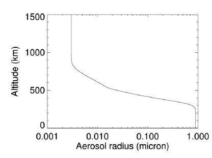
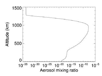
Figure 1: Aerosol properties from Lavvas et al. (2010) derived from a microphysical model validated against DISR observations. left: The mean radius of particles. right: The mixing ratio of particles.

2.1 Boundary Conditions

The lower boundary of our model is the surface of Titan and the upper boundary is at 1500 km. For H and H₂ the flux at the lower boundary is zero and at the top of the atmosphere these molecules are allowed to escape with velocities of 2.4 $\times$ 10⁴ cms^-1 and 6.1 $\times$ 10³ cms^-1 respectively (equivalent to fluxes of 3.78 $\times$ 10⁸ H atoms cm^-2 and 6.2 $\times$ 10⁹ H₂ molecules cm^-2). For all other gaseous species the concentration gradient at the lower boundary is assumed to be zero, while they have zero flux at the top boundary. Observations suggest that CH₄ can escape from the top of the atmosphere by sputtering (de La Haye et al., 2007) but the same effect can be generated in models by applying a larger eddy diffusivity (Li et al., 2015, 2014; Yelle et al., 2008) which is the approach we have taken here. Condensed species have zero flux at both the upper and lower boundaries.

Table 1 provides a list of the molecules in our model. The mixing ratio of N₂ is set according to the observational data and held fixed, with values below 50 km taken from the Huygens observations (Niemann et al., 2005) and above 1000 km from Cassini/UVIS data (Kammer et al., 2013). Between 50 and 1000 km the mixing ratio is assumed to be 0.98. The mixing ratio of CH₄ is fixed to the observed (super-saturated) values (Niemann et al., 2010) below the tropopause and allowed to vary above this.

Family	Molecule
	H, H2
hydrocarbons	C CH CH2 3CH2 CH3 CH4 C2 C2H C2H2 C2H3 C2H4 C2H5 C2H6 C3 C3H C3H2 C3H3 C2CCH2 CH3C2H C3H5 C3H6 C3H7 C3H8 C4H C4H2 C4H3 C4H4 C4H5 1-C4H6 1,2-C4H6 1,3-C4H6 C4H8 C4H9 C4H10 C5H3 C5H4 C6H C6H2 C6H3 C6H4 C6H5 $l$-C6H6 C6H6 C8H2
nitrogen-molecules	N NH NH2 NH3 N2H N2H2 N2H3 N2H4 CN HCN HNC H2CN CHCN CH2CN CH3CN C2H3CN C2H5CN C3H5CN C2N2 HC2N2 C3N HC3N HC4N CH3C2CN H2C3N C4N2 HC5N C6N2 CH2NH CH2NH2 CH3NH CH3NH2
condensed molecules	C2H${}_{2}^{c}$ C2H${}_{4}^{c}$ C2H${}_{6}^{c}$ CH2CCH${}_{2}^{c}$ CH3C2Hc C3H${}_{6}^{c}$ C3H${}_{8}^{c}$ C4H${}_{2}^{c}$ C4H${}_{4}^{c}$ 1-C4H6c 1,2-C4H6c 1,3-C4H6c C4H${}_{8}^{c}$ C4H${}_{10}^{c}$ C5H${}_{4}^{c}$ $l$-C6H${}_{6}^{c}$ C6H${}_{6}^{c}$ HCNc HNCc CH3CNc C2H3CNc C2H5CNc C3H5CNc C2N${}_{2}^{c}$ C4N${}_{2}^{c}$ C6N${}_{2}^{c}$ HC3Nc HC5Nc CH3C2CNc CH2NHc CH3NH${}_{2}^{c}$ NH${}_{3}^{c}$ N2H${}_{2}^{c}$ N2H${}_{4}^{c}$

Table 1: The species included in the model. A superscript of ^c indicates the molecule is condensed.

2.2 Condensation and Sublimation

Condensation occurs when the saturation ratio, $S$, of a molecule is greater than 1. S is defined as n($x$)/n_sat(s), where n($x$) is the gas phase mixing ratio of species $x$ and n_sat($x$) is its saturated density derived from the saturated vapor pressure. For $S$ $<$ 1, condensation is switched off and sublimation of any adsorbed molecules can occur. The abrupt change in behavior at $S$ = 1 can lead to numerical instabilities where the system oscillates between the condensation and sublimation regimes. In previous Titan models various methods have been used to smooth out the transition and prevent such instabilities. For example, Yung et al. (1984) parameterized the condensation rate in terms of $S$:

$$\hbox{Loss rate}\propto-\frac{S-1}{S}$$ (4)

This results in a relatively constant loss rate as a function of $S$. A more complicated expression was used by Lavvas et al. (2008a) to ensure that the loss rate increases with increasing saturation ratios:

$$\hbox{Loss rate}\propto-(S-1)\frac{exp(-0.5/ln(S+1)^{2})}{ln(S+1)^{2}}\hbox{~{}~{}~{}for S $>$ 1}$$ (5)

Other expressions that have been invoked include

$$\hbox{Loss rate}\propto-lnS$$ (6)

(Krasnopolsky, 2009).

Here we use a numerically stable method to determine the net condensation rate. The rate at which molecules condense on to a pre-existing aerosol particle is given by the collision rate with the particle:

$$k_{c}=\alpha_{x}\sigma v_{x}n(x)\hbox{~{}~{}~{}molecules s${}^{-1}$}$$ (7)

where $\alpha$ is the sticking coefficient of molecule $x$ (where $\alpha_{x}$ $\leq$ 1), $\sigma$ is the collisional cross-section of the particles, $v_{x}$ is the gas phase velocity of $x$, and $n(x)$ is its number density. For a pure ice the saturated vapor pressure is measured when the condensation and sublimation processes are in equilibrium. In this scenario

$$k_{c}n_{sat}(x)=k_{s}\Theta_{x}$$ (8)

where $k_{s}$ is the sublimation rate and $\Theta_{x}$ is the surface coverage of molecule $x$. In the case of a pure ice, $\Theta_{x}$ = 1, and hence the sublimation rate, $k_{s}$ = $k_{c}n_{sat}(x)$. The net condensation rate, $J_{c}$ is therefore

$$J_{c}=\alpha_{x}\sigma v_{x}[n(x)-n_{sat}(x)\Theta_{x}]\hbox{~{}~{}~{}molecules s${}^{-1}$}$$ (9)

When sublimation is taking place from a mixture of ices (rather than from pure ice) $\Theta$ will be less than 1 and the resulting gas phase abundance will be lower than the saturated value. $\Theta$ is calculated from

$$\Theta=n(x^{c})/\Sigma_{y}n(y^{c})$$ (10)

where $n(x^{c})$ is the number density of $x$ in the condensed phase, $\Sigma_{y}n(y^{c})$ is the total number density of all molecules condensed on to the grain surface. We assume that the ices are well-mixed, so that the composition of the surface from which sublimation occurs reflects that of the bulk of the ice.

To determine the saturated densities used in this paper we use the expressions for the saturated vapor pressure given in Table 2. The values from these fits are extrapolated as necessary to provide saturation vapor pressures over a wider range of temperatures. Figure 2 compares the predicted mixing ratios of HCN and C₂H₂ with the value predicted directly from the saturated vapor pressure. It can be seen that the model produces good agreement with the saturation vapor pressure in regions where the gas is saturated.

Molecule	Expression for log Psat	Temp range	Notes
	(mmHg)	(K)
CH4	6.84570 - 435.6214/(T-1.639)	91 – 189	Yaws (2007)
C2H2	6.09748 - (1644.1/T) + 7.42346 log(1000./T)	80 – 145	Moses et al. (1992)
	7.3147 - 790.20947/(T-10.141)	192 – 208	Lara et al. (1996)
C2H4	1.5477 - 1038.1 (1/T - 0.011) + 16537./(1/T - 0.011)2	77 – 89	Moses et al. (1992)
	8.724 - 901.6/(T-2.555)	89 –104	Moses et al. (1992)
	50.79 - 1703./T - 17.141 log(T)	104 – 120	Moses et al. (1992)
	6.74756 - 585./(T-18.18)	120 – 155	Moses et al. (1992)
C2H6	10.01 - 1085./(T - 0.561)	30 – 90	Lara et al. (1996)
	6.9534 - 699.10608/(T-12.736)	91 – 305	Yaws (2007)
CH3C2H	6.78485 - 803.72998/(T-43.92)	183 – 267	Yaws (2007)
CH2CCH2	6.62555 - 684.69623/(T-55.658)	144 – 294	Yaws (2007)
C3H6	6.8196 - 785./(T-26.)	161 – 241	Yaws (2007)
C3H8	7.0189 - 889.8642/(T-15.916)	85 – 176	Yaws (2007)
C4H2	5.3817 - 3300.5/T + 16.63415 log10(1000./T)	127–237	Lara et al. (1996)
	6.5326 - 761.68429/(T-74.732)	237 – 478	Yaws (2007)
C4H4	6.6633 - 826.0438/(T-59.712)	181 – 454	Yaws (2007)
1-C4H6	6.98198 - 988.75(T-39.99)	205 – 300	Yaws (2007)
1,2-C4H6	6.99383 - 1041.117/(T-30.726)	247 – 303	Yaws (2007)
1,3-C4H6	6.84999 - 930.546/(T-34.146)	215 – 287	Yaws (2007)
C4H8	6.8429 - 926.0998/(T-33.)	192 – 286	Yaws (2007)
C4H10	7.0096 - 1022.47681/(T-24.755)	135 – 425	Yaws (2007)
C5H4	7.986 - 1509.98716/(T-32.226)	234 – 367	Yaws (2007)
l-C6H6	7.95508 - 1773.77625/(T-52.937)	341 – 449	Yaws (2007)
C6H6	6.814 - 1090.43115/(T-75.852)	233 – 562	Yaws (2007)
NH3	7.5874 - 1013.78149/(T-24.17)	196 – 405	Yaws (2007)
HCN	11.41 - 2318./T	132 – 168	Lara et al. (1996)
	8.0258 - 1608.28491/(T-286.893)	260 – 456	Yaws (2007)
HNC	11.41 - 2318./T	132 – 168	same as HCN
	8.0258 - 1608.28491/(T-286.893)	260 – 456	same as HCN
C2N2	6.9442 - 779.237/(T-60.078)	146 – 400	Yaws (2007)
C4N2	8.269 - 2155./T	147 – 384	Yaws (2007)
C6N2	8.269 - 2155./T	147 – 384	same as C4N2
HC3N	6.2249 - 714.01178/(T-101.55)	214 – 315	Yaws (2007)
HC5N	6.2249 - 714.01178/(T-101.55)	214 – 315	same as HC3N
C2H3CN	7.8376 - 1482.7653/T-25.)	189 – 535	Yaws (2007)
C2H5CN	7.0414 - 1270.41907/(T-65.33)	204 – 564	Yaws (2007)
C3H5CN	7.0406 - 1617.87915/(T-34.032)	186 – 583	Yaws (2007)
N2H2	7.8288 - 1698.58081/(T-43.21)	270 – 653	same as N2H4
N2H4	7.8288 - 1698.58081/(T-43.21)	270 – 653	Yaws (2007)
CH3NH2	7.3638 - 1025.39819/(T-37.938)	180 – 430	Yaws (2007)
CH3CN	6.8376 - 995.2049/(T-80.494)	266 – 518	Yaws (2007)
CH3C2CN	6.2249 - 714.01178/(T-101.855)	214 – 315	Yaws (2007)
CH2NH	8.0913 - 1582.91077/(T-33.904)	175 –512	From Yaws (2007) value for CH3OH

Table 2: Expressions used to calculate the saturated vapor pressures. In the absence of laboratory data we assume that the saturated vapor pressure of HNC is the same as HCN, and that of N₂H₂ is the same as N₂H₄. We follow Loison et al. (2015) in using the vapor pressure of CH₃OH for CH₂NH and in using H₃CN for H₅CN.

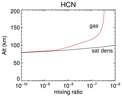
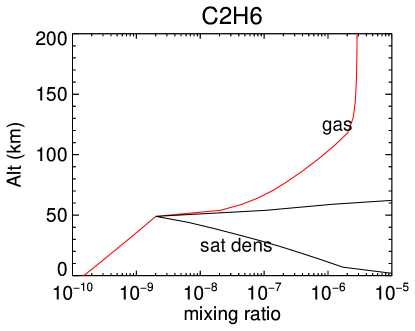
Figure 2: A comparison of the model results and the calculated mixing ratio under saturation conditions for (a) HCN and (b) C₂H₂. The saturated value (black line) is calculated assuming a pure ice and using the vapor pressure expressions given in Table 2. The model is shown in red. The two lines coincide in the region where the model calculations reach the saturated value and deviate where the calculated mixing ratios are below the saturated values.

2.3 Sedimentation and Haze Formation

We assume that the abundance, size and location of the aerosol particles is fixed. In reality the particles do not remain at the same altitude but rather sediment out towards the surface of Titan, taking any condensates with them. To mimic this effect we have included a loss process for condensed molecules which removes them from the model atmosphere with a rate coefficient of 10^-10 s^-1. All condensed species are assumed to be lost at the same rate. The assumed size of this reaction rate is somewhat arbitrary and to test the sensitivity of our results to its value we also considered a loss rate of 10^-12 molecules s^-1. Changing the rate was found to have no effect on the predicted gas phase mixing ratios.

In addition to the condensation of ice or liquids onto existing aerosols, molecules can also be incorporated into new or existing aerosols. In this scenario the molecules are then unavailable for return to the gas via sublimation and are permanently removed from the gas (Liang et al., 2007). This process is simulated using rates that are proportional to the collision rates between aerosols (assuming mean radii provided by Lavvas et al. (2010)) and molecules. We simulate this by adding reactions that remove the molecules from the gas with

$$\hbox{X}+haze=haze\hbox{~{}~{}~{}k = $\beta v\sigma n_{g}$ s${}^{-1}$}$$ (11)

where $n_{g}$ is the mixing ratio of aerosol particles, and $\beta$ is an efficiency factor ranging from 0.01 to 10 depending on the molecule. The value of $\beta$ was chosen for each molecule to maximize the agreement of the models with the observations. The molecules to be removed in this way are HCN ($\beta$ = 0.01), C₂H₃CN ($\beta$ = 0.1), HC₃N and HNC ($\beta$ = 10) C₂H₅CN ($\beta$ = 1). Other molecules are assumed not to condense in this way – for these molecules agreement of the models with observations is sufficiently good without invoking an additional loss mechanism such as haze formation.

3 Results

3.1 The Effect of Condensation Processes

We present the results of three models with different assumptions about the condensation and sublimation. Model A is a gas phase only model, with no condensation. Model B includes condensation and sublimation processes as outlined in Section 2.2, and the sedimentation of aerosol particles and their condensates. Model C extends Model B to include the removal of molecules from the gas by haze formation. The model parameters are summarized in Table 3.

Model	Condensation	Sedimentation	Haze
			formation
A	No	No	No
B	Yes	Yes	No
C	Yes	Yes	Yes

Table 3: Summary of model assumptions. Condensation and sublimation rates are discussed in Section 2.2. Sedimentation and haze formation rates are discussed in Section 2.3.

The largest effects are seen for the biggest molecules and in particular for those that contain nitrogen. The addition of sedimentation increases the rate of removal of these species from the gas in the lower atmosphere and improves agreement with the observations. However, some molecules are still found to be over-abundant. Further improvement is achieved between 200 and 600 km for HCN, HNC, HC₃N and C₂H₅CN if these molecules are assumed to be incorporated into haze particles.

Below we discuss the chemistry of several species in more detail.

3.2 Distribution of Nitrogen Molecules

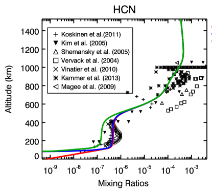
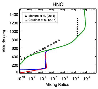
Figure 3: Distribution of some nitrogen-bearing molecules. (red line = Model A, blue line = Model B, green line = Model C). Cassini/INMS ($\bullet$ Cui et al. (2009); $\triangleleft$ Magee et al. (2009), $\Leftcircle$ Vuitton et al. (2007)), Cassini/UVIS (+ Koskinen et al. (2011), $\vartriangle$ Shemansky et al. (2005), $*$ Kammer (2015)), Keck ($\blacktriangledown$ Kim et al., 2005)), Voyager occultation observations ($\square$ Vervack et al. (2004)), Cassini/CIRS ($\times$ Vinatier et al. (2010), $\ocircle$Nixon et al. (2010), $\Diamondblack$ Teanby et al. (2013)), ($\blacktriangle$ Moreno et al., 2011), IRAM ($\diamond$ Marten et al. (2002)), ALMA ($\oplus$ Cordiner et al. (2014)).

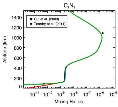
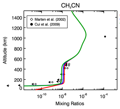
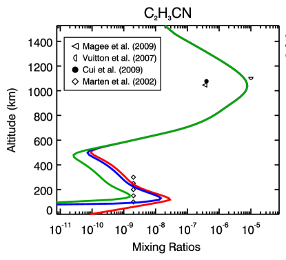
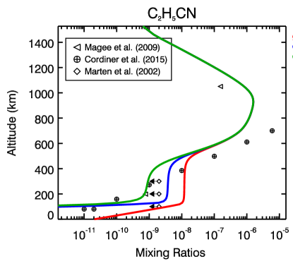
Figure 4: Abundances of more nitrogen-bearing species. Cassini/INMS ($\bullet$ Cui et al. (2009), $\triangleleft$ Magee et al. (2009), $\Leftcircle$ Vuitton et al. (2007)), Cassini/CIRS ($\Diamondblack$ Teanby et al. (2013)), IRAM 30m ($\diamond$ Marten et al. (2002)), ALMA data ($\oplus$ Cordiner et al. (2015)).

3.2.1 NH₃

In the lower atmosphere upper limits of the NH₃ abundance are provided by Herschel/SPIRE measurements (65 – 100 km; Teanby et al., 2013) and from CIRS/Cassini limb observations (110 – 250 km; Nixon et al., 2010). In the upper atmosphere the abundance is derived from Cassini/INMS of NH${}_{4}^{+}$ (Vuitton et al., 2007) at 1100 km. Cui et al. (2009) claim a detection of NH₃ in the ionosphere between 950 and 1200km. Their value is an order of magnitude larger than that derived by Vuitton et al. and its origin is a matter of debate. It is possible that this high value is due to spent hydrazine fuel (Magee et al., 2009).

Our model abundances in the upper atmosphere are a factor of 10 lower than the observations of Vuitton et al. (2007) (Figure 3). Below 250 km our models are considerably lower (but consistent with) the upper limits derived by Teanby et al. (2013) and Nixon et al. (2010).

The main formation processes for NH₃ are

$$\hbox{C${}_{2}$H${}_{3}$}+\hbox{NH${}_{2}$} \longrightarrow\hbox{NH${}_{3}$}+\hbox{C${}_{2}$H${}_{2}$} <$$ 800 km (12)

with destruction by photodissociation.

As discussed by Loison et al. (2015) the formation of NH₃ via neutral-neutral reactions depends on the presence of NH₂ which is not efficiently produced in Titan’s atmosphere. The inclusion of ion-molecule chemistry may lead to higher abundances of NH₃.

3.2.2 HCN

Observations of HCN have been made from 100 km to 1000 km. The millimeter observations of Marten et al. (2002) covered the whole disk and were mainly sensitive to the mid-latitude and equatorial regions. Observations from Cassini/CIRS (Vinatier et al., 2007, 2010), UVIS (Koskinen et al., 2011; Shemansky et al., 2005; Kammer, 2015), and INMS (Magee et al., 2009) provide abundance information between 400 and 1000 km. Abundances in the lower atmosphere are also provided by Kim et al. (2005) from Keck observations (Geballe et al., 2003). Vervack et al. (2004) used Voyager 1 Ultraviolet Spectrometer measurements to determine abundances between 500 and 900km, although the inferred abundances are much higher than other estimates. The differences between the Voyager 1 HCN abundances and those from Cassini may be due to solar cycle variations. Investigating such differences is beyond the scope of this work.

Overall our models are in good agreement with the observational data (Figure 3). We find that condensation and sublimation are important for HCN below 500 km. The best fit to the observations is obtained with Model C (Figure 3), where sedimentation and haze formation reduce the abundance of HCN below 500 km.

The main formation processes are

$$\hbox{HNC}+\hbox{H} \longrightarrow\hbox{HCN}+\hbox{H}$$ 300 – 800 km (13)

$$\hbox{CN}+\hbox{CH${}_{4}$} \longrightarrow\hbox{HCN}+\hbox{CH${}_{3}$}$$ 200 – 600 km (14)

$$\hbox{N}+\hbox{CH${}_{2}$} \longrightarrow\hbox{HCN}+\hbox{H}$$ 600 – 900 km (15)

$$\hbox{C${}_{2}$H${}_{3}$CN}+h\nu \longrightarrow\hbox{HCN}+\hbox{C${}_{2}$H${}_{2}$} <$$ 1000 km (16)

$$\hbox{H${}_{2}$CN}+\hbox{H} \longrightarrow\hbox{HCN}+\hbox{H}_{2}$$ 900 - 1300 km (17)

Photodissociation plays a role in both the formation of HCN (via photodisssociation of C₂H₃CN above 1000 km) and in its destruction (forming CN and H). Below 200 km destruction is by

$$\hbox{C${}_{2}$H${}_{3}$}+\hbox{HCN}\longrightarrow\hbox{C${}_{2}$H${}_{3}$CN}+\hbox{H}$$ (18)

3.2.3 HNC

The first observations of HNC in Titan were made using Herschel/HIFI by Moreno et al. (2011). These measurements do not allow the exact vertical abundance profile to be determined. Several possible profiles can fit the data depending on the mixing ratio and the cut-off altitude assumed. Loison et al. (2015) suggest two possible profiles: one where the mixing ratio of HNC is 1.4 $\times$10^-5 above 900 km (shown in Figure 3) and another where the mixing ratio is 6 $\times$10^-5 above 1000 km. Our models fall between these two ranges.

More recently Cordiner et al. (2014) used ALMA to detect HNC. They found that the emission mainly originates at altitudes above 400 km and that there are two emission peaks that are not symmetrical in longitude. We are able to match their best fit profile reasonably well with model C (green line; Figure 3), where HNC forms haze providing the best agreement with the data at lower altitudes.

The main formation channels of HNC are

$$\hbox{C${}_{2}$H${}_{3}$CN}+h\nu \longrightarrow\hbox{HNC}+\hbox{C${}_{2}$H${}_{2}$} <$$ 900 km (19)

$$\hbox{H${}_{2}$CN}+\hbox{H} \longrightarrow\hbox{HNC}+\hbox{H${}_{2}$} >$$ 900 km (20)

$$\hbox{N}+\hbox{CH${}_{3}$} \longrightarrow\hbox{HNC}+\hbox{H} >$$ 900 km (21)

The main destruction process is by reaction with H atoms forming HCN. This reaction has an activation barrier. In the literature the value for the activation barrier ranges from 800 to 2000 K (Talbi et al., 1996; Sumathi & Nguyen, 1998; Petrie, 2002; Wakelam et al., 2012). Here we are using the rate from the KIDA database (Wakelam et al., 2012) which has the highest activation barrier of 2000 K. Loison et al. (2015) used the lowest value (800 K), resulting in more efficient HCN production and consequently a lower gas phase abundance of HNC than we see here. We find that reducing the activation barrier does indeed reduce the mixing ratio of HNC but does not result in a good fit to the ALMA observations in this region (Figure 5).

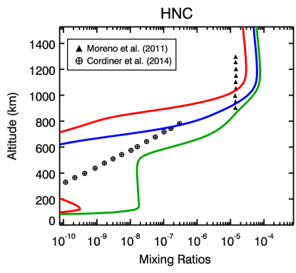
Figure 5: How the HNC abundance depends on the activation barrier of the reaction H + HNC $\longrightarrow$ HCN + H. green E_A = 2000 K (Wakelam et al., 2012), blue E_A = 1400 K, red E_A = 800 K (Loison et al., 2015). The lower activation barrier results in more HNC being converted into HCN but does not result in a better agreement with the altitude distribution seen in the ALMA observations.

3.2.4 HC₃N

HC₃N has been observed at altitudes from 200 to 1000 km (Marten et al., 2002; Vervack et al., 2004; Teanby et al., 2006; Vuitton et al., 2007; Cui et al., 2009; Magee et al., 2009; Vinatier et al., 2010; Cordiner et al., 2014). Below 500 km our models are in excellent agreement with the observations if it is assumed that HC₃N forms aerosols and thus is permanently removed from the gas (Figure 3 (bottom left)). Condensation and sublimation alone result in an over-estimate of the abundance compared to the observations in this region. Good agreement is also seen for all models between 500 km and 700 km. Above this our models tend to under predict the HC₃N abundance. Below 100 km the mixing ratio follows the saturation level, so that below this altitude the mixing ratio is much reduced compared to the gas only model. Better agreement with the observations below 400 km is obtained in the haze formation model where condensed molecules are assumed to be incorporated into aerosol particles and removed from the gas.

The main formation process below 1000 km is

$$\hbox{C${}_{3}$N}+\hbox{CH${}_{4}$}\longrightarrow\hbox{HC${}_{3}$N}+\hbox{CH}_{3}$$ (22)

and above 800 km by

$$\hbox{CN}+\hbox{C${}_{2}$H${}_{2}$} \longrightarrow\hbox{HC${}_{3}$N}+\hbox{H}$$ (23)

$$\hbox{C${}_{2}$H${}_{3}$CN}+h\nu \longrightarrow\hbox{HC${}_{3}$N}+\hbox{H}_{2}$$ (24)

Destruction is by photodissociation

$$\hbox{HC${}_{3}$N}+h\nu\longrightarrow\hbox{C${}_{3}$N}+\hbox{H}$$ (25)

and by reaction with H atoms

$$\hbox{H}+\hbox{HC${}_{3}$N}+\hbox{M}\longrightarrow\hbox{H${}_{2}$C${}_{3}$N}+\hbox{M}$$ (26)

The observations show a sharp decrease in the abundance of HC₃N below 400 km. In our models this can be accounted for if HC₃N is incorporated into haze particles (Model C). An alternative explanation of meridional circulation and condensation in the polar regions has been suggested (Loison et al., 2015; Hourdin et al., 2004).

3.2.5 C₂N₂

Observations of C₂N₂ have been made by Cassini/CIRS (Teanby et al., 2006, 2009) and by Cassini/INMS (Cui et al., 2009; Magee et al., 2009). The models with condensation are in very good agreement with both of these datasets (Figure 4). Without condensation the abundance in the lower atmosphere is over-estimated.

The main formation route for C₂N₂ is by the reaction of CN and HNC:

$$\hbox{CN}+\hbox{HNC}\longrightarrow\hbox{C${}_{2}$N${}_{2}$}+\hbox{H}$$ (27)

with destruction via photodissociation forming CN or by

$$\hbox{H}+\hbox{C${}_{2}$N${}_{2}$}+\hbox{M}\longrightarrow\hbox{H${}_{2}$CN${}_{2}$}+\hbox{M}\hbox{~{}~{}~{}~{}$<$ 400 km}$$ (28)

3.2.6 CH₃CN

Submillimeter observations with the IRAM 30 m telescope detected the CH₃CN (12-11) rotational line providing a disk average vertical profile up to 500 km, dominated by the equatorial region (Marten et al., 2002). Cassini/CIRS (Nixon et al., 2013) and Cassini/INMS (Vuitton et al., 2007; Cui et al., 2009) provide estimates of the abundance above 1000 km.

All models are in good agreement with the observations below 800 km, although all predict slightly lower abundances than observed between 500 and 600 km. The predicted mixing ratio at 1100 km is a factor of 10 lower than the observed value of 3 $\times$10^-5 Cui et al. (2009).

The main formation processes are

$$\hbox{CN}+\hbox{CH}_{4} \longrightarrow\hbox{CH${}_{3}$CN}+\hbox{H} <$$ 900 km (29)

$$\hbox{NH}+\hbox{C${}_{2}$H${}_{4}$} \longrightarrow\hbox{CH${}_{3}$N}+\hbox{H} >$$ 900 km (30)

$$\hbox{CH${}_{2}$NH}+\hbox{CH} =\hbox{CH${}_{3}$CN}+\hbox{H} <$$ 900 km (31)

with destruction by

$$\hbox{CH${}_{3}$CN}+\hbox{H} \longrightarrow\hbox{CN}+\hbox{CH}_{4} <$$ 1200 km (32)

3.2.7 C₂H₃CN

Several observations have placed upper limits on the abundance of C₂H₃CN. Marten et al. (2002) used the IRAM 30m telescope to determine upper limits between 100 and 300 km. Cassini/INMS has provided an upper limit of 4 $\times$10^-7 at 1077 km (Cui et al., 2009), while Cassini/INMS Magee et al. (2009) determined a mixing ratio of 3.5 $\times$10^-7 at 1050 km and Vuitton et al. (2007) found 10^-5 at 1100 km from observations of ions. Cordiner et al. (private communication) have detected C₂H₃CN in the submillimeter and found an average abundance of 1.9 x 10^-9 above 300 km.The model abundance of C₂H₃CN in the upper atmosphere is within a factor of 2 of the Vuitton et al. (2007) value but 50 times higher than Magee et al. (2009) and Cui et al. (2009).

None of our models have a constant mixing ratio with altitude between 100 and 300 km as derived from the IRAM observations (Figure 4). Model B and C (which include condensation) are consistent with the derived mixing ratio at a particular altitude, but neither reproduce the constant value between 100 and 300 km. In the upper atmosphere all models predict mixing ratios within a factor a 3 of the Magee et al. (2009) result but are over-abundant compared to the other measurement in this region.

The main production mechanism is by reaction of CN with C₂H₄:

$$\hbox{C${}_{2}$H${}_{3}$}+\hbox{HCN} \longrightarrow\hbox{C${}_{2}$H${}_{5}$CN}+\hbox{H} <$$ 200 km (33)

$$\hbox{CN}+\hbox{C${}_{2}$H${}_{4}$} \longrightarrow\hbox{C${}_{2}$H${}_{3}$CN}+\hbox{H}$$ 400 – 800 km (34)

$$\hbox{H${}_{2}$C${}_{3}$N}+\hbox{H} \longrightarrow\hbox{C${}_{2}$H${}_{3}$CN} >$$ 400 km (35)

Gas phase destruction processes are

$$\hbox{C${}_{2}$H${}_{3}$CN}+h\nu \longrightarrow\left\{\begin{array}[]{ll}\hbox{HCN}+\hbox{C${}_{2}$H${}_{2}$}\\ \hbox{HNC}+\hbox{C${}_{2}$H${}_{2}$}\\ \hbox{HC${}_{3}$N}+\hbox{H}_{2}\end{array}\right.$$ (39)

Below 400 km haze formation and sedimentation of aerosol particles play an important role in determining the gas mixing ratio in Model C.

3.2.8 C₂H₅CN

Upper limits for the abundance of C₂H₅CN have been determined between 100 and 300 km from IRAM 30m observations Marten et al. (2002), with abundances in the upper atmosphere provided by Cassini/INMS data (Vuitton et al., 2007; Cui et al., 2009; Magee et al., 2009). More recently Cordiner et al. (2015) detected this molecule above 200 km using ALMA.

Our models over-estimate the abundance of C₂H₅CN in the upper atmosphere (Figure 4), probably because we do not include ion chemistry (for a discussion of this point see Loison et al., 2015). Below 700 km, Model C is in excellent agreement with the ALMA data of Cordiner et al.

The main formation process is

$$\hbox{CH${}_{2}$CN}+\hbox{CH${}_{3}$}+\hbox{M}\longrightarrow\hbox{C${}_{2}$H${}_{5}$CN}+\hbox{M}$$ (40)

Destruction is by photodissociation

$$\hbox{C${}_{2}$H${}_{5}$CN}+h\nu \longrightarrow\left\{\begin{array}[]{ll}\hbox{C${}_{2}$H${}_{4}$}+\hbox{HCN}\\ \hbox{CH}_{3}+\hbox{CH${}_{2}$CN}\\ \hbox{C${}_{2}$H${}_{3}$CN}+\hbox{H${}_{2}$}\end{array}\right.$$ (44)

or by reaction with CH, C₂H₃ or C₂H.

$$\hbox{C${}_{2}$H${}_{5}$CN}+\hbox{CH} \longrightarrow\hbox{CH${}_{2}$CN}+\hbox{C${}_{2}$H${}_{4}$}$$ (45)

$$\hbox{C${}_{2}$H${}_{5}$CN}+\hbox{C${}_{2}$H} \longrightarrow\hbox{HC${}_{3}$N}+\hbox{C${}_{2}$H${}_{5}$} <$$ 300 km (46)

$$\hbox{C${}_{2}$H${}_{3}$CN}+\hbox{C${}_{2}$H${}_{3}$} \longrightarrow\hbox{C${}_{2}$H${}_{3}$CN}+\hbox{C${}_{2}$H${}_{5}$} <$$ 300 km (47)

3.3 Condensates in Titan’s Atmosphere

We find several layers at which condensates are abundant with the location being molecule dependent. The first condensate layer is in the lower atmosphere around the tropopause. Here we find condensates of C₂H₂, C₂H₄, C₂H₆, C₃H₈ among others. A little further up in the atmosphere around 65 – 80 km several molecules have peaks in condensation e.g. HCN, C₄H₈, C₄H₂, C₂H₃CN, C₂N₂, CH₃C₂H. Another layer of C₂H₃CN, CH₃CN, C₂H₅CN and CH₃C₂H forms around 110 – 130 km. Several molecules also have high condensation levels between 600 and 900 km e.g. CH₃C₂H, HC₅N, HC₃N, CH₃CN, and C₂H₅CN. Figure 6 shows the condensation layers for HCN and HC₃N. Both these molecules have high condensate abundances between 70 and 100 km, but HC₃N has a further peak around 500 km where the atmospheric temperature dips, and the gas phase abundance of this molecule is high.

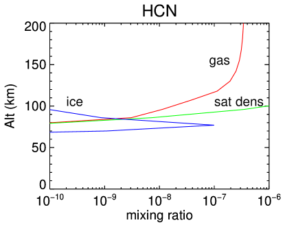
Figure 6: The calculated mixing ratios of HCN (left) and HC₂N (right) in the gas (red line) and in condensed form (blue line). Also shown is the saturated mixing ratio (green line). The mixing ratio of HCN^c peak at $\sim$ 65 km. The mixing ratio of HCN in the gas around this altitude is slightly below the saturated value, even though there is condensed HCN available to be sublimated. The reason for this is that the condensates are not pure. Since the sublimation rate depends on the surface coverage of the condensed molecule sublimation from a mixed condensate is less efficient than from a pure condensate, leading to lower gas abundances. A similar effect is seen for other condensed molecules. For HC₃N the peak condensate mixing ratio occurs around 500 km where there is a dip in temperature corresponding to a high local abundance of HC₃N. Other nitrogen-bearing molecules show similar behavior in this region.

The net flux of material falling on to the surface of Titan can be calculated from the difference between the atmospheric formation and destruction. Table 4 presents our predictions of the surface flux of nitrogen molecules. These are in solid form and if evenly distributed across Titan’s surface would create a layer 4.4 m deep over a timescale of 1 Gyr. This amount of “fixed nitrogen” could be of biological importance.

Molecule	Flux	Flux	Depth (m)	Solid/Liquid
	(molecules cm-2 s-1)	(g cm-2/Gyr)		at 95 K
HCNc	-1.2 $\times$108	-170	2.12	S
HNCc	-8.1 $\times$106	-11.0	0.14	S
HC3Nc	-2.9 $\times$107	-77.4	1.0	S
HC5Nc	-3.4  106	-13.5	0.17
C2N${}_{2}^{c}$	-5.8 $\times$105	-15.8	0.02	S
CH3CNc	-2.8 $\times$105	-0.6	0.01	S
CH3C2CN	-4.5 $\times$106	-15.3	0.19
C2H5CNc	-6.4 $\times$106	-18.4	0.23	S
C2H3CNc	-1.5 $\times$107	-41.6	0.52	S
Total N			4.4 m

Table 4: Flux of condensed molecules onto Titan’s surface. Also shown are the estimated deposit thickness (depths) calculated assuming an average density of 0.8 g cm^-3.

4 Discussion and Conclusions

The removal of molecules by condensation plays an important role in determining the gas phase composition of Titan’s atmosphere, as well as creating new aerosols. Condensates are found throughout the atmosphere. For the majority of molecules, condensation is most efficient below the tropopause. Larger molecules, and in particular nitrogen-bearing molecules have another condensation peak between 200 and 600 km. Relatively high abundances of condensates can also be present above 500 km if the gas phase abundance of a given molecule is high, e.g. HC₃N, HC₅N, CH₃CN and C₂H₅CN. These molecules condense in the region where Titan’s haze forms. The effect is enhanced if it is assumed that some molecules can be permanently removed from the gas by being incorporated into aerosol particles. This mechanism was able to bring the abundances of HC₃N, HCN, HNC, CH₃CN and C₂H₅CN into good agreement with the observations below 600 km.

Although Titan possesses a rich organic chemistry it is unclear whether this could lead to life. Photochemically produced compounds on Titan, principally acetylene, ethane and organic solids, would release energy when consumed with atmospheric hydrogen, which is also a photochemical product. McKay & Smith (2005) speculate on the possibility of widespread methanogenic life in liquid methane on Titan. On Earth fixed nitrogen is often a limiting nutrient. Our work shows that an abundant supply of fixed nitrogen, including species of considerable complexity, is available from atmospheric photochemistry.

Creating the kinds of lipid membranes that form the basis of lie on Earth depends on the presence of liquid water. Titan’s atmosphere contains little oxygen and the surface temperature is well below that at which liquid water can survive. Instead surface liquids are hydrocarbons (e.g. Hayes, 2016). Therefore any astrobiological processes, if present, are likely to be quite different to those on Earth. A recent paper by Stevenson et al. (2015) suggests that as alternative to lipids, membranes could be formed from small nitrogen-bearing organic molecules such as acrylonitrile (C₂H₃CN). Stevenson et al. calculate that a membrane composed of acrylonitrile molecules would be thermodynamically stable at cryogenic temperatures and would have a high energy barrier to decomposition.

All of our models predict abundances of C₂H₃CN that are in agreement with observations above 500 km. Below this condensation and incorporation into haze are required to bring the predicted mixing ratios down to the values inferred from observations Cordiner et al. (2015). If acrylonitrile were to be involved in life formation it needs to reach the surface of Titan. Our predicted flux of this molecule onto Titan’s surface is 1.5 $\times$10⁷ molecules cm^-2 s^-1, or $\sim$ 41.5 gcm^-2/Gyr, a quantity that is potentially of biological importance.

References

- Allen et al. (1981) Allen, M., Yung, Y. L., & Waters, J. W. 1981, J. Geophys. Res., 86, 3617
- Anderson et al. (2016) Anderson, C. M., Samuelson, R. E., Yung, Y. L., & McLain, J. L. 2016, Geophys. Res. Letts., 43, 3088
- Cordiner et al. (2014) Cordiner, M. A., Nixon, C. A., Teanby, N. A., et al. 2014, Astrophys. J. Letts, 795, L30
- Cordiner et al. (2015) Cordiner, M. A., Palmer, M. Y., Nixon, C. A., et al. 2015, Astrophys. J. Letts, 800, L14
- Coustenis & Taylor (1999) Coustenis, A., & Taylor, F. 1999, Titan : the earth-like moon (Singapore: World Scientific)
- Cui et al. (2009) Cui, J., Yelle, R. V., Vuitton, V., et al. 2009, Icarus, 200, 581
- De La Haye et al. (2008) De La Haye, V., Waite, J. H., Cravens, T. E., Robertson, I. P., & Lebonnois, S. 2008, Icarus, 197, 110
- de La Haye et al. (2007) de La Haye, V., Waite, J. H., Johnson, R. E., et al. 2007, Journal of Geophysical Research (Space Physics), 112, A07309
- Geballe et al. (2003) Geballe, T. R., Kim, S. J., Noll, K. S., & Griffith, C. A. 2003, Astrophys. J. Letts, 583, L39
- Gladstone et al. (2016) Gladstone, G. R., Stern, S. A., Ennico, K., et al. 2016, Science, 351, aad8866
- Hayes (2016) Hayes, A. G. 2016, Annual Review of Earth and Planetary Sciences, 44, 57
- Hourdin et al. (2004) Hourdin, F., Lebonnois, S., Luz, D., & Rannou, P. 2004, Journal of Geophysical Research (Planets), 109, E12005
- Kammer (2015) Kammer, J. A. 2015, PhD thesis, California Institute of Technology
- Kammer et al. (2013) Kammer, J. A., Shemansky, D. E., Zhang, X., & Yung, Y. L. 2013, Planet. Space Sci., 88, 86
- Kim et al. (2005) Kim, S. J., Geballe, T. R., Noll, K. S., & Courtin, R. 2005, Icarus, 173, 522
- Koskinen et al. (2011) Koskinen, T. T., Yelle, R. V., Snowden, D. S., et al. 2011, Icarus, 216, 507
- Krasnopolsky (2009) Krasnopolsky, V. A. 2009, Icarus, 201, 226
- Lara et al. (1996) Lara, L. M., Lellouch, E., López-Moreno, J. J., & Rodrigo, R. 1996, J. Geophys. Res., 101, 23261
- Lavvas et al. (2010) Lavvas, P., Yelle, R. V., & Griffith, C. A. 2010, Icarus, 210, 832
- Lavvas et al. (2008a) Lavvas, P. P., Coustenis, A., & Vardavas, I. M. 2008a, Planet. Space Sci., 56, 27
- Lavvas et al. (2008b) —. 2008b, Planet. Space Sci., 56, 67
- Li et al. (2015) Li, C., Zhang, X., Gao, P., & Yung, Y. 2015, Astrophys. J. Letts, 803, L19
- Li et al. (2014) Li, C., Zhang, X., Kammer, J. A., et al. 2014, Planet. Space Sci., 104, 48
- Liang et al. (2007) Liang, M.-C., Yung, Y. L., & Shemansky, D. E. 2007, Astrophys. J. Letts, 661, L199
- Loison et al. (2015) Loison, J. C., Hébrard, E., Dobrijevic, M., et al. 2015, Icarus, 247, 218
- Lorenz & Mitton (2008) Lorenz, R., & Mitton, J. 2008, Titan Unveiled: Saturn’s Mysterious Moon Explored (Princeton University Press)
- Lunine (2005) Lunine, J. I. 2005, in Meteorites, Comets and Planets: Treatise on Geochemistry, ed. A. M. Davis (Elsevier B), 623
- Magee et al. (2009) Magee, B. A., Waite, J. H., Mandt, K. E., et al. 2009, Planet. Space Sci., 57, 1895
- Marten et al. (2002) Marten, A., Hidayat, T., Biraud, Y., & Moreno, R. 2002, Icarus, 158, 532
- McKay & Smith (2005) McKay, C. P., & Smith, H. D. 2005, Icarus, 178, 274
- Moreno et al. (2011) Moreno, R., Lellouch, E., Lara, L. M., et al. 2011, Astron. Astrophys., 536, L12
- Moses et al. (1992) Moses, J. I., Allen, M., & Yung, Y. L. 1992, Icarus, 99, 318
- Niemann et al. (2005) Niemann, H. B., Atreya, S. K., Bauer, S. J., et al. 2005, Nature, 438, 779
- Niemann et al. (2010) Niemann, H. B., Atreya, S. K., Demick, J. E., et al. 2010, J. Geophys. Res. (Planets), 115, 12006
- Nixon et al. (2010) Nixon, C. A., Achterberg, R. K., Teanby, N. A., et al. 2010, Faraday Discussions, 147, 65
- Nixon et al. (2013) Nixon, C. A., Jennings, D. E., Bézard, B., et al. 2013, Astrophys. J. Letts, 776, L14
- Petrie (2002) Petrie, S. 2002, J. Phys. Chem. A, 106, 11181
- Shemansky et al. (2005) Shemansky, D. E., Stewart, A. I. F., West, R. A., et al. 2005, Science, 308, 978
- Stern et al. (2015) Stern, S. A., Bagenal, F., Ennico, K., et al. 2015, Science, 350, aad1815
- Stevenson et al. (2015) Stevenson, J., Lunine, J., & Clancy, P. 2015, Science Advances, 1, 1400067
- Strobel (1974) Strobel, D. F. 1974, Icarus, 21, 466
- Sumathi & Nguyen (1998) Sumathi, R., & Nguyen, M. 1998, J. Phys. Chem. A, 102, 8013–8020
- Talbi et al. (1996) Talbi, D., Ellinger, Y., & Herbst, E. 1996, A&A, 314, 688
- Teanby et al. (2009) Teanby, N. A., Irwin, P. G. J., de Kok, R., et al. 2009, Icarus, 202, 620
- Teanby et al. (2006) —. 2006, Icarus, 181, 243
- Teanby et al. (2013) Teanby, N. A., Irwin, P. G. J., Nixon, C. A., et al. 2013, Planet. Space Sci., 75, 136
- Vervack et al. (2004) Vervack, R. J., Sandel, B. R., & Strobel, D. F. 2004, Icarus, 170, 91
- Vinatier et al. (2007) Vinatier, S., Bézard, B., Fouchet, T., et al. 2007, Icarus, 188, 120
- Vinatier et al. (2010) Vinatier, S., Bézard, B., Nixon, C. A., et al. 2010, Icarus, 205, 559
- Vuitton et al. (2007) Vuitton, V., Yelle, R. V., & McEwan, M. J. 2007, Icarus, 191, 722
- Wakelam et al. (2012) Wakelam, V., Herbst, E., Loison, J.-C., et al. 2012, Astrophys. J. Suppl., 199, 21
- Westlake et al. (2011) Westlake, J. H., Bell, J. M., Waite, Jr., J. H., et al. 2011, J. Geophys. Res. (Space Phys.), 116, 3318
- Wilson & Atreya (2004) Wilson, E. H., & Atreya, S. K. 2004, J. Geophys. Res., 106, 2181
- Yaws (2007) Yaws, C. L. 2007, Yaws handbook of vapor pressures: Antoine Coefficients (Houston, Tex: Gulf Pub.)
- Yelle et al. (2008) Yelle, R. V., Cui, J., & Müller-Wodarg, I. C. F. 2008, Journal of Geophysical Research (Planets), 113, E10003
- Yung et al. (1984) Yung, Y. L., Allen, M., & Pinto, J. P. 1984, Astrophys. J. Suppl., 55, 465