Evaluation of toroidal torque by non-resonant magnetic perturbations in tokamaks for resonant transport regimes using a Hamiltonian approach

Abstract

Toroidal torque generated by neoclassical viscosity caused by external non-resonant, non-axisymmetric perturbations has a significant influence on toroidal plasma rotation in tokamaks. In this article, a derivation for the expressions of toroidal torque and radial transport in resonant regimes is provided within quasilinear theory in canonical action-angle variables. The proposed approach treats all low-collisional quasilinear resonant NTV regimes including superbanana plateau and drift-orbit resonances in a unified way and allows for magnetic drift in all regimes. It is valid for perturbations on toroidally symmetric flux surfaces of the unperturbed equilibrium without specific assumptions on geometry or aspect ratio. The resulting expressions are shown to match existing analytical results in the large aspect ratio limit. Numerical results from the newly developed code NEO-RT are compared to calculations by the quasilinear version of the code NEO-2 at low collisionalities. The importance of the magnetic shear term in the magnetic drift frequency and a significant effect of the magnetic drift on drift-orbit resonances are demonstrated.

I Introduction

In tokamaks, non-axisymmetric magnetic field perturbations such as toroidal field ripple, error fields and perturbation fields from Edge Localized Mode (ELM) mitigation coils produce non-ambipolar radial transport at non-resonant flux surfaces occupying most of the plasma volume. The toroidal torque associated with this transport significantly changes the toroidal plasma rotation – an effect known as neoclassical toroidal viscosity Zhu et al. (2006); Shaing et al. (2009a); Park et al. (2009); Shaing et al. (2010); Kasilov et al. (2014); Shaing et al. (2015) (NTV). At low collisionalities, resonant transport regimes Yushmanov (1982, 1990), namely superbanana plateau Shaing et al. (2009b); Shaing (2015), bounce and bounce-transit (drift-orbit) resonance regimes Shaing et al. (2009a), have been found to play an important role in modern tokamaks, in particular in ASDEX Upgrade Martitsch et al. (2016). In these regimes, which emerge if perturbation field amplitudes are small enough, transport coefficients become independent of the collision frequency (form a plateau). The interaction of particles with the (quasi-static) electromagnetic field in these plateau-like regimes is a particular case of collisionless wave-particle interaction with time dependent fields and can be described within quasilinear theory. The most compact form of this theory in application to a tokamak geometry is obtained in canonical action-angle variables Kaufman (1972); Hazeltine et al. (1981); Mahajan et al. (1983); Becoulet et al. (1991); Timofeev and Tokman (1994); Kominis et al. (2008). Here, this formalism is applied to ideal quasi-static electromagnetic perturbations, which can be described in terms of flux coordinates. As a starting point, the Hamiltonian description of the guiding center motion in those coordinates in general 3D magnetic configurations (see, e.g., Refs. White et al., 1982; White and Chance, 1984; White, 1990) is used. For the particular case of Boozer coordinates the perturbation theory is constructed with respect to non-axisymmetric perturbations of the magnetic field module, which is the only function of angles relevant for neoclassical transport.

The purpose of this paper is twofold: The first aim is to describe the NTV in all quasilinear resonant regimes in a unified form using the standard Hamiltonian formalism and to develop a respective numerical code allowing for fast NTV evaluation in these regimes without any simplifications to the magnetic field geometry. The second aim is to benchmark this approach with the quasilinear version of the NEO-2 code Kasilov et al. (2014); Martitsch et al. (2016) which treats the general case of plasma collisionality. Since particular resonant regimes described in literature basically agree with the Hamiltonian approach within their applicability domains, such a benchmarking means also the benchmarking of NEO-2 against those results. The structure of the paper is as follows. In section II, basic definitions are given and two different quasilinear expressions for the toroidal torque density are derived for the general case of small amplitude quasi-static electromagnetic perturbations. In section III the perturbation theory for ideal perturbations described by small corrugation of magnetic surfaces in flux coordinates is outlined, and expressions for the canonical action-angle variables are given. In section IV expressions for non-axisymmetric transport coefficients are derived, and in section V the numerical implementation of the Hamiltonian formalism in the code NEO-RT is presented and its results compared with the results of NEO-2 code for typical resonant transport regimes. The results are summarized in section VI.

II Transport equations and toroidal torque in Hamiltonian variables

In Hamiltonian variables the kinetic equation can be compactly written in the form

$$\frac{\partial f}{\partial t}+\left\{f,H\right\}=\hat{L}_{c}f,$$ (1)

where $\hat{L}_{c}$ is the collision operator and

$$\left\{f,g\right\}\equiv\frac{\partial f}{\partial{\bf r}}\cdot\frac{\partial g}{\partial{\bf p}}-\frac{\partial f}{\partial{\bf p}}\cdot\frac{\partial g}{\partial{\bf r}}=\frac{\partial f}{\partial\theta^{i}}\frac{\partial g}{\partial J_{i}}-\frac{\partial f}{\partial J_{i}}\frac{\partial g}{\partial\theta^{i}}=\frac{\partial}{\partial\theta^{i}}\left(f\frac{\partial g}{\partial J_{i}}\right)-\frac{\partial}{\partial J_{i}}\left(f\frac{\partial g}{\partial\theta^{i}}\right)$$ (2)

is the Poisson bracket which is invariant with respect to the canonical variable choice. Here, $({\bf r},{\bf p})$ are Cartesian coordinates and canonical momentum components, $(\boldsymbol{\theta},{\bf J})$ are canonical angles and actions specified later, summation over repeated indices is assumed, and bold face describes a whole set of three variables (e.g. $\boldsymbol{\theta}=(\theta^{1},\theta^{2},\theta^{3})$). In the following derivations, straight field line flux coordinates ${\bf x}=(r,\vartheta,\varphi)$ are used with a specific definition of the flux surface label (effective radius) such that $\langle|\nabla r|\rangle=1$, where the neoclassical magnetic flux surface average is given by

$$\langle a\rangle=\frac{1}{S}\int\limits_{-\pi}^{\pi}{\rm d}\vartheta\int\limits_{-\pi}^{\pi}{\rm d}\varphi\;\sqrt{g}\;a,\qquad S=\int\limits_{-\pi}^{\pi}{\rm d}\vartheta\int\limits_{-\pi}^{\pi}{\rm d}\varphi\;\sqrt{g},$$ (3)

and $\sqrt{g}$ is the metric determinant. Due to the above definition of $r$, quantity $S$ has the meaning of the flux surface area.

Multiplying (1) by a factor $a\,\delta\left(r-r_{c}\right)$ where $a=a(\boldsymbol{\theta},{\bf J})=a({\bf r},{\bf p})$ is some function of particle position in the phase space and $r_{c}=r_{c}(\boldsymbol{\theta},{\bf J})=r({\bf r}_{c}(\boldsymbol{\theta},{\bf J}))$ is the particle effective radius expressed via phase space variables, integrating over the phase space and dividing the result by the flux surface area $S$ leads to a generalized conservation law

$$\frac{\partial A}{\partial t}+\frac{1}{S}\frac{\partial}{\partial r}S\Gamma_{A}=s_{A}+s_{A}^{(c)},$$ (4)

where

$$A=A(t,r) \equiv \frac{1}{S}\int{\rm d}^{3}\theta\int{\rm d}^{3}J\;\delta\left(r-r_{c}\right)af=\frac{1}{S}\int{\rm d}^{3}r\delta\left(r-r_{c}\right)\int{\rm d}^{3}p\;af$$ (5)

$$= \frac{1}{S}\int\limits_{-\pi}^{\pi}{\rm d}\vartheta\int\limits_{-\pi}^{\pi}{\rm d}\varphi\;\sqrt{g}\int{\rm d}^{3}p\;af=\left\langle\int{\rm d}^{3}p\;af\right\rangle,$$

where $\delta(\dots)$ is the Dirac delta function. Generalized magnetic surface averaged flux and source densities in (4) are given, respectively, by

$$\Gamma_{A} \equiv \frac{1}{S}\int{\rm d}^{3}\theta\int{\rm d}^{3}J\;\delta\left(r-r_{c}\right)\left\{r_{c},H\right\}af,$$ (6)

$$s_{A} \equiv \frac{1}{S}\int{\rm d}^{3}\theta\int{\rm d}^{3}J\;\delta\left(r-r_{c}\right)\left\{a,H\right\}f,$$ (7)

where the second representation of the Poisson bracket (2) has been used for these expressions, and the collisional source density is

$$s_{A}^{(c)}=\left\langle\int{\rm d}^{3}p\;a\hat{L}_{c}f\right\rangle.$$ (8)

For $a=1$ the continuity equation is obtained with no sources, $s_{n}=s_{n}^{(c)}=0$ and surface averaged particle flux density $\Gamma_{A}=\Gamma$ given by

$$\Gamma=\frac{1}{S}\int{\rm d}^{3}\theta\int{\rm d}^{3}J\;\delta\left(r-r_{c}\right)\left\{r_{c},H\right\}f.$$ (9)

For $a=p_{\varphi}$ with

$$p_{\varphi}={\bf p}\cdot\frac{\partial{\bf r}}{\partial\varphi}=m_{\alpha}v_{\varphi}+\frac{e_{\alpha}}{c}A_{\varphi}(r)$$ (10)

being the canonical angular momentum, the equation for the canonical angular momentum density is obtained with the source term $s_{a}=s_{p_{\varphi}}=T_{\varphi}^{\rm NA}$ being the toroidal torque density acting on the given species from the electromagnetic field,

$$T_{\varphi}^{\rm NA}=-\frac{1}{S}\int{\rm d}^{3}\theta\int{\rm d}^{3}J\;\delta\left(r-r_{c}\right)\frac{\partial H}{\partial\varphi}f.$$ (11)

In Eq. (10), $v_{\varphi}={\bf v}\cdot\partial{\bf r}/\partial\varphi$ and $A_{\varphi}=-\psi_{\rm pol}$ are covariant toroidal velocity and vector potential components, respectively and $\psi_{\rm pol}$ is the normalized poloidal flux. In addition, speed of light $c$, and charge $e_{\alpha}$ and mass $m_{\alpha}$ of species $\alpha$ appear in the expression.

One can see that torque density is determined only by the non-axisymmetric part of the distribution function while the particle flux density contains also the axisymmetric contribution. This property of the torque is rather helpful in the nonlinear transport theory which, however, is not the topic of the present paper. A conservation law of the kinematic toroidal momentum, $a=m_{\alpha}v_{\varphi}$, is obtained by subtraction of the continuity equation multiplied by $e_{\alpha}A_{\varphi}/c$. The source term in this equation is

$$s_{m_{\alpha}v_{\varphi}}=T_{\varphi}^{\rm NA}+s_{p_{\varphi}}^{(c)}+\frac{e_{\alpha}}{c}\sqrt{g}B^{\vartheta}\Gamma,$$ (12)

where $B^{\vartheta}$ is the poloidal contravariant magnetic field component. Assuming a static momentum balance and estimating $\Gamma_{m_{\alpha}v_{\varphi}}\sim m_{\alpha}v_{\varphi}\Gamma$, which means that contribution of the radial momentum transport term to this balance is negligible because it scales to the last term in (12) as $q\rho_{L}R/r^{2}\ll 1$, this balance is reduced to $s_{m_{\alpha}v_{\varphi}}=0$. Here $q$, $\rho_{L}$, $R$ and $r$ are safety factor, Larmor radius, major and minor radius, respectively. The result is a flux-force relation Hirshman (1978); Shaing and Callen (1983), which links particle flux to the torques (a static density equilibrium without particle sources where $\Gamma=0$ demonstrates the fact that $T_{\varphi}^{\rm NA}$ is indeed a torque density because it balances collisional momentum source density $s_{p_{\varphi}}^{(c)}$ alone). The presence of the collisional force moment $s_{p_{\varphi}}^{(c)}$ in the flux force relation indicates that the calculation of torque and radial flux needs a certain caution when using a Krook collision model, which is usually the case in quasilinear “collisionless” plateau transport regimes described here. Due to momentum conservation by collisions, collisional torque $s_{p_{\varphi}}^{(c)}$ provides no contribution to the total torque that is of main interest here, which is not ensured by the simple Krook model. This is the case, in particular, for the ion component in the simple plasma where momentum is largely conserved within this component. Thus, when computing particle flux density in this case, one should keep in mind that direct computation of $\Gamma$ from the quasilinear equation provides a different result as compared to such computation through $T_{\varphi}^{\rm NA}$ via the flux force relation with no collisional torque $s_{p_{\varphi}}^{(c)}$,

$$T_{\varphi}^{\rm NA}=-\frac{e_{\alpha}}{c}\sqrt{g}B^{\vartheta}\Gamma=-\frac{e_{\alpha}}{c}\frac{{\rm d}\psi_{{\rm pol}}}{{\rm d}r}\Gamma.$$ (13)

Since $T_{\varphi}^{\rm NA}$ is not affected by details of the collision model, this more appropriate definition of $\Gamma$ is assumed below unless otherwise mentioned. It should be noted that in the standard neoclassical theory Hinton and Hazeltine (1976) momentum conservation terms are usually treated first before any approximations on the collision operator are made thus avoiding the errors of the kind discussed above.

Further steps are standard for quasilinear theory in action-angle variables Kaufman (1972). One presents the Hamiltonian and the distribution function as a sum of the unperturbed part depending on actions only and a perturbation with zero average over canonical angles, $H(\boldsymbol{\theta},{\bf J})=H_{0}({\bf J})+\delta H(\boldsymbol{\theta},{\bf J})$ and $f(\boldsymbol{\theta},{\bf J})=f_{0}({\bf J})+\delta f(\boldsymbol{\theta},{\bf J})$, respectively and expands the perturbations into a Fourier series over canonical angles,

$$\delta H(\boldsymbol{\theta},{\bf J})=\sum_{\bf m}H_{\bf m}({\bf J}){\rm e}^{im_{k}\theta^{k}},\qquad\delta f(\boldsymbol{\theta},{\bf J})=\sum_{\bf m}f_{\bf m}({\bf J}){\rm e}^{im_{k}\theta^{k}},$$ (14)

where sums exclude ${\bf m}=(0,0,0)$ term. By using a Krook collision term with infinitesimal collisionality, $\hat{L}_{c}f=-\nu\delta f\rightarrow 0$, the amplitudes of the perturbed distribution function from the linear order equation follow as

$$\left\{\delta f,H_{0}\right\}+\left\{f_{0},\delta H\right\}+\nu\delta f=\sum_{\bf m}\left(\left(im_{k}\Omega^{k}+\nu\right)f_{\bf m}-iH_{\bf m}m_{k}\frac{\partial f_{0}}{\partial J_{k}}\right){\rm e}^{im_{k}\theta^{k}}=0.$$ (15)

Here, $\Omega^{k}=\partial H/\partial J_{k}$ are canonical frequencies, and the time derivative has been omitted as small compared to all canonical frequencies in case of quasi-static perturbations of interest here. A quasilinear equation is obtained by retaining only secular, angle-independent terms in the second order equation,

$$\frac{\partial f_{0}}{\partial t}+\overline{\left\{\delta f,\delta H\right\}}=\frac{\partial f_{0}}{\partial t}-\sum_{\bf m}m_{k}\frac{\partial Q_{\bf m}}{\partial J_{k}}=0,$$ (16)

where the over-line stands for the average over the angles, and

$$Q_{{\bf m}}=Q_{{\bf m}}({\bf J})=\frac{\pi}{2}|H_{{\bf m}}|^{2}\delta(m_{j}\Omega^{j})m_{k}\frac{\partial f_{0}}{\partial J_{k}}$$ (17)

contains a resonance condition in the argument of a delta function that follows from the limit $\nu\rightarrow 0$. The knowledge of $f_{\bf m}$ is already sufficient for the evaluation of torque densities from Eq. (11) where the derivative over $\varphi$ is equivalent to a derivative over the canonical toroidal phase $\theta^{3}$,

$$T^{\rm NA}_{\varphi}=-\frac{m_{3}}{S}\int d^{3}\theta\int d^{3}J\delta(r-r_{c})\sum_{\bf m}Q_{\mathbf{m}},$$ (18)

and of the particle flux from (9)

$$\Gamma_{\rm F}=-\frac{1}{S}\int d^{3}\theta\int d^{3}J\delta(r-r_{c})\sum_{\mathbf{m}}m_{k}\frac{\partial r_{c}}{\partial J_{k}}Q_{\mathbf{m}},$$ (19)

which is distinguished here from (13) by subscript $F$. Alternatively the same expressions are obtained computing the conservation laws using the quasilinear equation (16) as a starting point Hazeltine et al. (1981). If the collision model does not conserve the parallel momentum such as e.g. the Krook model, direct calculations of the torque in terms of viscosity Shaing et al. (2009a) and calculation of the torque through particle flux Park et al. (2009) using the force-flux relation (13) may lead to different results. This difference, however, is negligible in resonant transport regimes where details of the collision model are not important, and collisionality can be treated as infinitesimal.

III Tokamak with ideal non-axisymmetric quasi-static perturbations

III.1 Canonical Hamiltonian variables for perturbed equilibria

Often in quasilinear theory in action-angle variables, both, the unperturbed and perturbed Hamiltonian correspond to physically possible motion with separation of the unperturbed electromagnetic field and its perturbation in real space. However, there is no mathematical need to do so. In particular, if the perturbed equilibrium is ideal such that it can be described in flux coordinates, it is more convenient to restrict the perturbations only to those quantities in the Hamiltonian which violate the axial symmetry. In case of Boozer coordinates and also in many cases described in Hamada coordinates the only important quantity is the magnetic field module which is generally adopted for the construction of perturbation theory for NTV models Shaing et al. (2009a); Park et al. (2009); Shaing et al. (2010); Kasilov et al. (2014); Shaing (2015). Thus the guiding center Lagrangian Littlejohn (1983) is transformed here to flux coordinates ${\bf x}=(r,\vartheta,\varphi)$ as a starting point,

$$L=m_{\alpha}v_{\parallel}h_{r}\dot{r}+(m_{\alpha}v_{\parallel}h_{\vartheta}+\frac{e_{\alpha}}{c}A_{\vartheta})\dot{\vartheta}+(m_{\alpha}v_{\parallel}h_{\varphi}+\frac{e_{\alpha}}{c}A_{\varphi})\dot{\varphi}+J_{\perp}\dot{\phi}-H,$$ (20)

where lower subscripts denote covariant components (in particular, $A_{\vartheta}=A_{\vartheta}(r)=\psi_{\rm tor}$ is the covariant poloidal component of the vector potential, which is equal to the normalized toroidal flux and $A_{r}=0$), $\mathbf{h}=\mathbf{B}/B$ is the unit vector along the magnetic field, $v_{\parallel}$ is the parallel velocity, $J_{\perp}=m_{\alpha}v_{\perp}^{2}/(2\omega_{c})$ is the perpendicular adiabatic invariant with $v_{\perp}$ and $\omega_{c}$ being the perpendicular velocity and cyclotron frequency, respectively, $\phi$ is the gyrophase and the Hamiltonian is given explicitly below in Eq. (26). The canonical form of the Lagrangian is obtained by transforming the toroidal angle $\varphi$ to

$$\varphi_{H}=\varphi-\frac{cm_{\alpha}v_{\parallel}h_{r}}{e_{\alpha}A_{\varphi}^{\prime}},$$ (21)

where the prime stands for a radial derivative. Omitting a total time derivative, the Lagrangian transforms to

$$L=p_{\vartheta}\dot{\vartheta}+p_{\varphi}\dot{\varphi}_{H}+J_{\perp}\dot{\phi}-H+\frac{cm_{\alpha}^{2}v_{\parallel}h_{\varphi}}{e_{\alpha}}\frac{d}{dt}\left(\frac{v_{\parallel}h_{r}}{A_{\varphi}^{\prime}}\right),$$ (22)

where

$$p_{\vartheta}=m_{\alpha}v_{\parallel}h_{\vartheta}({\bf x})+\frac{e_{\alpha}}{c}A_{\vartheta}(r),\qquad p_{\varphi}=m_{\alpha}v_{\parallel}h_{\varphi}({\bf x})+\frac{e_{\alpha}}{c}A_{\varphi}(r)$$ (23)

are canonical momenta in guiding center approximation, and the last term is of the next order in $\rho_{\parallel}=v_{\parallel}/\omega_{c}$ and should therefore be neglected. Transformation (21) affects only a small non-axisymmetric part of the field and is different from the one of Refs. White and Chance (1984); White (1990) where the poloidal angle $\vartheta$ is modified instead. Alternatively, for collisionless transport regimes of interest here, one can simply ignore the covariant magnetic field component $B_{r}$ because it does not contribute to the radial guiding center velocity, and its contribution to the rotation velocity vanishes on a time scale larger than bounce time.

Since the momenta are the independent variables, Eq. (23) should be regarded as a definition of $r$ and $v_{\parallel}$. For the construction of perturbation theory in Boozer coordinates being the main choice here, the last quantity is redefined via the unperturbed parallel velocity $v_{0\parallel}$ as follows,

$$v_{\parallel}=v_{0\parallel}\frac{B({\bf x})}{B_{0}(r,\vartheta)}$$ (24)

where subscript 0 corresponds to the axisymmetric part of the respective quantity. Due to such redefinition, $r$ and $v_{0\parallel}$ do not depend on the toroidal angle $\varphi$ because in Boozer coordinates this dependence vanishes in both expressions in (23) due to $h_{\vartheta,\varphi}=B_{\vartheta,\varphi}(r)/B({\bf x})$. For the comparison with the results obtained in Hamada coordinates for the superbanana-plateau regime, which is a resonant regime described by the bounce-averaged equation, the definition of the unperturbed parallel velocity is opposite to (24), $v_{\parallel}=v_{0\parallel}B_{0}/B$. With this redefinition, angular covariant components of ${\bf h}$ in (24) are transformed within linear order in the perturbation field as follows,

$$Bh_{k}=B_{0}h_{0k}+\frac{\partial\delta\chi}{\partial x^{k}}-h_{0k}h_{0}^{j}\frac{\partial\delta\chi}{\partial x^{j}},\qquad k=2,3,$$ (25)

where $\delta\chi$ is the non-axisymmetric perturbation of a function $\chi$ which enters the definition of co-variant magnetic field components in Hamada coordinates $B_{k}$ via their flux surface averages $\bar{B}_{k}=\bar{B}_{k}(r)$, with $B_{k}=\bar{B}_{k}+\partial\chi/\partial x^{k}$. Terms with $\delta\chi$, whose contribution in (25) is orthogonal to the unperturbed magnetic field, can be simply ignored in bounce-averaged regimes because they do not contribute to bounce averaged velocity components.

Thus, the Hamiltonian is expanded in Boozer coordinates up to a linear order in the perturbation field amplitude as follows,

$$H=\omega_{c}J_{\perp}+\frac{m_{\alpha}v_{\parallel}^{2}}{2}+e_{\alpha}\Phi=\frac{B}{B_{0}}\omega_{c0}J_{\perp}+\frac{B^{2}}{B_{0}^{2}}\frac{m_{\alpha}v_{0\parallel}^{2}}{2}+e_{\alpha}\Phi\approx H_{0}+\delta H,$$ (26)

where $\Phi=\Phi(r)$ is the electrostatic potential,

$$H_{0}=\omega_{c0}J_{\perp}+\frac{m_{\alpha}v_{0\parallel}^{2}}{2}+e_{\alpha}\Phi,\qquad\delta H=\left(\omega_{c0}J_{\perp}+m_{\alpha}v_{0\parallel}^{2}\right)\frac{\delta B}{B_{0}}.$$ (27)

The Hamiltonian perturbation $\delta H$ in Hamada coordinates differs from (27) by the opposite sign of the second term in the parentheses, $m_{\alpha}v_{0\parallel}^{2}$. This term is usually ignored in tokamaks with large aspect ratio $A$ because for trapped and barely trapped particles which are mainly contributing to NTV at small Mach numbers (at sub-sonic toroidal rotation velocities) it scales to the first term as $1/A$.

III.2 Action-angle variables in the axisymmetric tokamak

Since this subsection deals only with unperturbed motion corresponding to $H=H_{0}$, the subscript 0 is dropped on all quantities here which are strictly axisymmetric. Here it is convenient to replace the toroidal momentum $p_{\varphi}$, which is now a conserved quantity, by another invariant of motion $r_{\varphi}$ which describes the banana tip radius for trapped particles Hazeltine et al. (1981) and is implicitly defined via

$$\frac{e_{\alpha}}{c}A_{\varphi}(r_{\varphi})=p_{\varphi}.$$ (28)

Expanding the vector potential components in (23) over $r-r_{\varphi}$ up to the linear order and using $A^{\prime}_{\vartheta}/A^{\prime}_{\varphi}=-{\rm d}\psi_{\rm tor}/{\rm d}\psi_{\rm pol}=-q$, the poloidal momentum is approximated by

$$p_{\vartheta}=\frac{e_{\alpha}}{c}A_{\vartheta}+\frac{m_{\alpha}v_{\parallel}}{h^{\vartheta}}.$$ (29)

In the above formula and in the remaining derivation, all quantities are evaluated at $r=r_{\varphi}$ if not noted otherwise. In this approximation it is possible to express derivatives with respect to $p_{\varphi}$ by radial derivatives. The poloidal action is defined for trapped $(\delta_{\rm t-p}=0)$ and passing $(\delta_{\rm t-p}=1)$ particles by

$$J_{\vartheta}=\frac{1}{2\pi}\oint d\vartheta p_{\vartheta}=\frac{e_{\alpha}}{c}A_{\vartheta}\delta_{\rm t-p}+J_{\parallel}.$$ (30)

The first term cancels when integrating back and forth between the turning points of a trapped orbit. The parallel adiabatic invariant may be written as a bounce average,

$$J_{\parallel}=\frac{m_{\alpha}\tau_{b}}{2\pi}\left\langle v_{\parallel}^{2}\right\rangle_{b},$$ (31)

with bounce time $\tau_{b}$, orbit time $\tau$ and bounce averaging $\left\langle a(\vartheta)\right\rangle_{b}$ defined by

$$\tau_{b} =\oint\frac{dl}{v_{\parallel}}=\oint\frac{d\vartheta}{v_{\parallel}h^{\vartheta}},$$ (32)

$$\tau(\vartheta_{0},\vartheta_{{\rm orb}}) =\int_{\vartheta_{0}}^{\vartheta_{{\rm orb}}}\frac{d\vartheta}{v_{\parallel}h^{\vartheta}},$$ (33)

$$\left\langle a(\vartheta)\right\rangle_{b} =\frac{1}{\tau_{b}}\oint\frac{d\vartheta}{v_{\parallel}h^{\vartheta}}a(\vartheta)=\frac{1}{\tau_{b}}\int_{0}^{\tau_{b}}d\tau\,a(\vartheta_{{\rm orb}}(\vartheta_{0},\tau)).$$ (34)

Here $a(\vartheta)$ is any function of the poloidal angle and integrals of motion $(J_{\perp},H_{0},s_{\varphi})$ and $\vartheta_{{\rm orb}}(\vartheta_{0},\tau)$ is the (periodic) solution of the unperturbed guiding center equations (the orbit) starting at the magnetic field minimum point $\vartheta_{0}$. Finally, we arrive at the expressions for the three canonical actions in a tokamak Kaufman (1972),

$$J_{1} =J_{\perp}=\frac{m_{\alpha}c}{e}\mu,$$

$$J_{2} =J_{\vartheta}=\frac{e_{\alpha}}{c}A_{\vartheta}\delta_{\rm t-p}+\frac{m_{\alpha}\tau_{b}}{2\pi}\left\langle v_{\parallel}^{2}\right\rangle_{b},$$

$$J_{3} =p_{\varphi}=m_{\alpha}v_{\parallel}h_{\varphi}+\frac{e_{\alpha}}{c}A_{\varphi},$$ (35)

where $\mu$ denotes the magnetic moment. Canonical frequencies $\Omega^{k}=\partial H/\partial J_{k}$ are

$$\Omega^{1}=\left\langle\omega_{c}\right\rangle_{b},\qquad\Omega^{2}=\omega_{b},\qquad\Omega^{3}=q\omega_{b}\delta_{\rm t-p}+\left\langle v_{g}^{\varphi}\right\rangle_{b},$$ (36)

where the bounce frequency $\omega_{b}=2\pi/\tau_{b}$ is strictly positive for trapped particles, whereas for passing particles it can take both, positive and negative values. The bounce average of the toroidal precession frequency $v_{g}^{\varphi}$ due to the cross-field drift is separated in two parts,

$$\left\langle v_{g}^{\varphi}\right\rangle_{b}\equiv\Omega_{t}=\left\langle\frac{v_{\parallel}}{\omega_{c}\sqrt{g}}\frac{\partial}{\partial r}\left(\frac{v_{\parallel}}{h^{\vartheta}}\right)\right\rangle_{b}=\left<\Omega_{tE}\right>_{b}+\left<\Omega_{tB}\right>_{b}.$$ (37)

Here, bounce averages of electric drift frequency $\Omega_{tE}$ and magnetic drift frequency $\Omega_{tB}$ are

$$\left<\Omega_{tE}\right>_{b} =\Omega_{tE}=-\frac{c}{\psi_{{\rm pol}}^{\prime}}\frac{\partial\Phi}{\partial r},$$

$$\left<\Omega_{tB}\right>_{b} =\frac{v^{2}}{\psi_{{\rm pol}}^{\prime}}\left<-\frac{2-\eta B}{2\omega_{c}}\frac{\partial B}{\partial r}+\frac{1-\eta B}{\omega_{c}}h^{\vartheta}\left(\frac{\partial B_{\vartheta}}{\partial r}+q\frac{\partial B_{\varphi}}{\partial r}+B_{\varphi}\frac{dq}{dr}\right)\right>_{b},$$ (38)

with equilibrium potential $\Phi$, and velocity space parameterized by velocity module $v$ and the parameter $\eta=v_{\perp}^{2}/(v^{2}B)=2e_{\alpha}J_{\perp}/(cm_{\alpha}^{2}v^{2})$. Comparison of magnetic rotation frequency $\left<\Omega_{tB}\right>_{b}$ given by Eq. (38) with the expression obtained by bounce averaging of Eq. (67) of Ref. Kasilov et al., 2014 one can notice the absence in the latter expression of a term $B_{\varphi}q^{\prime}(r)$ describing the magnetic shear. This results from using the local neoclassical ansatz as a starting point in the linearized equation for the non-Maxwellian perturbation of the distribution function where the radial derivative of this perturbation is ignored. This local ansatz is the standard method in drift kinetic equation solvers in general 3D toroidal geometries Hirshman et al. (1986); Landreman et al. (2014) and is justified in most transport regimes, but not in resonant regimes, where magnetic drift plays a significant role. As shown in the example below, the shear term may lead to a significant modification of the superbanana resonance condition. This term is retained if linearization is applied after bounce-averaging the kinetic equation Shaing (2015). It should be noted that the guiding center Lagrangian (20) used as a starting point here is valid for the general case of the magnetic field, which is not necessarily a force-free field. Therefore, the effects of finite plasma pressure on the toroidal rotation velocity Connor et al. (1983) are automatically taken into account in (38).

The canonical angles in the leading order follow as

$$\theta^{1}=\phi-\Delta\phi(\theta^{2},{\bf J}),\qquad\theta^{2}=\Omega^{2}\tau,\qquad\theta^{3}=\varphi_{H}+q\theta^{2}\delta_{\rm t-p}-q\vartheta_{{\rm orb}}(\vartheta_{0},\tau),$$ (39)

where $\Delta\phi$ is a periodic function of the canonical poloidal variable $\theta^{2}$. Since according to (39) $\phi$ and $\varphi_{H}$ differ from the respective canonical angles $\theta^{1}$ and $\theta^{3}$ by additional terms depending on $\theta^{2}$ only and $\vartheta$ depends only on $\theta^{2}$, the spectrum $a_{\mathbf{m}}$ in canonical angles of a function given by a single harmonic (l,n) of the original angles $\phi,\varphi$,

$$a(\phi,\vartheta,\varphi)=a_{ln}(\vartheta)e^{i\left(l\phi+n\varphi\right)}=\sum_{\mathbf{m}}a_{\mathbf{m}}e^{im_{k}\theta^{k}},$$ (40)

contains non-zero contributions only from canonical modes with $m_{1}=l$ and $m_{3}=n$. In particular, for the gyroaverage $\left\langle a\right\rangle_{g}$ described by the harmonic $l=0$ of function $a$, one obtains to the leading order in $\rho_{\parallel}$

$$a_{\bf m}=\left\langle a_{0n}(\vartheta)e^{inq\vartheta-i\left(m_{2}+nq\delta_{\rm t-p}\right)\omega_{b}\tau}\right\rangle_{b},$$ (41)

where ${\bf m}=(0,m_{2},n)$.

IV Neoclassical toroidal viscous torque and related radial transport

For NTV applications, where the perturbed Hamiltonian (27) is independent of gyrophase, only harmonics with first canonical mode number $m_{1}=0$ can contribute to fulfill the resonance condition inside the $\delta$ distribution of Eq. (17), and the latter is reduced to

$$m_{j}\Omega^{j}=0\,\,\,\rightarrow\,\,\,(m_{2}+nq\delta_{\rm t-p})\omega_{b}+n\Omega_{t}=0.$$ (42)

This equation includes all regimes of interest here: The superbanana-plateau resonance is described by the condition $m_{2}=0$ for trapped particles. For passing particles, $m_{2}=0$ corresponds to a transit resonance. This is the only resonance remaining in the infinite aspect ratio limit, where it reduces to the usual Cherenkov (TTMP) resonance. Finite mode numbers $m_{2}$ correspond to bounce and bounce-transit resonances for trapped and passing particles, respectively. Resonances where both, parallel motion and cross-field drift determine the resonance condition, i.e. all resonances except the superbanana-plateau resonance are mentioned below as “drift-orbit” resonances.

Due to the properties of the spectrum (40), which follow from the axial symmetry of the unperturbed field, separate toroidal harmonics of perturbation Hamiltonian produce independent contributions to the torque and particle flux density. Therefore it is sufficient to assume the perturbation field $\delta B$ in (27) in the form of a single toroidal harmonic,

$$\delta B={\rm Re}(B_{n}(\vartheta)e^{in\varphi}).$$ (43)

Making use of Eq. (41), the associated modes of the Hamiltonian perturbation result in

$$H_{\mathbf{m}}=\left\langle\left(m_{\alpha}v_{0\parallel}^{2}(\vartheta)+\frac{e_{\alpha}}{m_{\alpha}c}J_{\perp}B_{0}(\vartheta)\right)\frac{B_{n}(\vartheta)}{B_{0}(\vartheta)}e^{inq\vartheta-i\left(m_{2}+nq\delta_{\rm t-p}\right)\omega_{b}\tau}\right\rangle_{b}.$$ (44)

For small enough perturbations, which are considered here, quasilinear effects are weak and thus $f_{0}$ is close to a drifting Maxwellian,

$$f_{0}=\frac{n_{\alpha}}{\left(2\pi m_{\alpha}T_{\alpha}\right)^{3/2}}e^{(e_{\alpha}\Phi-H_{0})/T_{\alpha}},$$ (45)

with parameters depending on $r_{\varphi}$ but not $r$. This Maxwellian differs from a local Maxwellian by linear terms in $\rho_{\parallel}$, which, as shown below, provide negligible contributions in resonant regimes with quasi-static perturbations. Let us check that within first order in $\rho_{\parallel}$ the toroidally drifting Maxwellian Eq. (45) is a solution to the axisymmetric kinetic equation for ions valid in all collisionality regimes in the absence of temperature gradients. For this purpose it is more convenient to replace the approximate expression for the canonical angular momentum (35) valid in first order in Larmor radius by the exact expression,

$$p_{\varphi}=m_{\alpha}v_{\varphi}+\frac{e_{\alpha}}{c}A_{\varphi},$$ (46)

where $v_{\varphi}$ is the toroidal covariant component of the total particle velocity including the Larmor gyration and $A_{\varphi}$ is evaluated at the exact particle position $r_{\rm c}$ (not at the guiding center position denoted with $r$ here) related to $r_{\varphi}$ as follows,

$$r_{\rm c}=r_{\varphi}+\frac{cm_{\alpha}v_{\varphi}}{e_{\alpha}\sqrt{g}B^{\vartheta}}.$$ (47)

Then, the unperturbed distribution function (45) up to linear order in Larmor radius is

$$f_{0}=\frac{n_{\alpha}}{\left(2\pi m_{\alpha}T_{\alpha}\right)^{3/2}}\exp\left(-\frac{m_{\alpha}}{2T_{\alpha}}\left({\bf v}_{\rm pol}^{2}+g_{\varphi\varphi}\left(v^{\varphi}-V_{\alpha}^{\varphi}\right)^{2}\right)\right),$$ (48)

where $g_{\varphi\varphi}=R^{2}$ and all functions of radius are evaluated at $r_{c}$. Here, ${\bf v}_{\rm pol}$ and $v^{\varphi}$ are total poloidal and contra-variant component of the total toroidal particle velocity, respectively, and the contra-variant toroidal component of the ion flow velocity is explicitly given by

$$V_{\alpha}^{\varphi}=\frac{c}{\sqrt{g}B^{\vartheta}}\left(E_{r}-\frac{T_{\alpha}}{e_{\alpha}n_{\alpha}}\frac{\partial n_{\alpha}}{\partial r_{c}}\right).$$ (49)

In a simple plasma where the momentum is approximately conserved within a single ion component, the drifting Maxwellian (48) annihilates the collision term. As a straightforward consequence of (48), the poloidal ion flow velocity is zero at all collisionalities if the temperature gradient is absent. Respectively, the toroidal flow velocity (49) is the same as given by ideal MHD (see, e.g., Eq. (6) of Ref. Kasilov et al., 2014). In the presence of temperature gradients and in a multi-species plasma Eq. (45) satisfies the kinetic equation only in zero order over Larmor radius. Additional anisotropic terms which appear in the first order solution are of same order as in (45), nevertheless, they provide a negligible contribution for the following reason. When substituting (45) in (17) one can notice that only derivatives of the parameters over $r_{\varphi}$ provide non-zero contributions in presence of resonance condition,

$$\delta(m_{j}\Omega^{j})m_{k}\frac{\partial f_{0}}{\partial J_{k}}=-\delta(m_{j}\Omega^{j})\frac{nc(A_{1}+A_{2}u^{2})}{e_{\alpha}}\frac{{\rm d}r}{{\rm d}\psi_{\rm pol}}f_{0},$$ (50)

where $u=v/v_{T}$ is the velocity module $v$ normalized by the thermal velocity $v_{T}=\sqrt{2T_{\alpha}/m_{\alpha}}$ and

$$A_{1}=\frac{1}{n_{\alpha}}\frac{\partial n_{\alpha}}{\partial r}+\frac{e_{\alpha}}{T_{\alpha}}\frac{\partial\Phi}{\partial r}-\frac{3}{2T_{\alpha}}\frac{\partial T_{\alpha}}{\partial r},\qquad A_{2}=\frac{1}{T_{\alpha}}\frac{\partial T_{\alpha}}{\partial r},$$ (51)

are the thermodynamic forces which are evaluated at $r=r_{\varphi}$. For any function $F$ of actions expressed in the form $F=F(H_{0},J_{\perp},p_{\varphi})$, only the derivative over $p_{\varphi}$ remains in expressions such as (50) because the derivative over $J_{1}$ enters with factor $m_{1}=0$ only, and the derivative over $H_{0}$ enters with factor $m_{k}\Omega^{k}$ which is zero due to the resonance condition (42) (the energy is preserved for static perturbations). Therefore the contribution of the linear correction in $\rho_{\parallel}$ to the unperturbed distribution function which depends also on $J_{\perp}$ would contribute in (50) only in the form of its derivative over $r_{\varphi}$ which is of higher order in $\rho_{\parallel}$ than such a derivative of the Maxwellian retained in (50). In the expression for the torque density (18) one can ignore finite Larmor radius effects together with finite orbit width effects in $r_{c}$ in the argument of the $\delta$-function by setting $r_{c}\approx r_{\varphi}$. Then an integration over $J_{3}=p_{\varphi}$ results in a replacement of $r_{\varphi}$ by $r$ in the subintegrand, and the integration over canonical angles is simply replaced by a factor $8\pi^{3}$. Changing the integration variables of the remaining integral over $J_{1}$ and $J_{2}$ to $v$ and $\eta$ and transforming the resulting $T_{\varphi}^{\rm NA}$ to a particle flux density using the flux-force relation (13) results in

$$\Gamma=\frac{2\pi^{2}nm_{\alpha}^{3}c}{e_{\alpha}S}\int_{0}^{\infty}dv\,v^{3}\int_{0}^{1/B_{{\rm min}}}d\eta\tau_{b}\sum_{{\rm m}_{2}}Q_{\mathbf{m}}.$$ (52)

Substituting $Q_{\mathbf{m}}$ in (52) explicitly and using the representation of $\Gamma$ in terms of thermodynamic forces (51), $\Gamma=-n_{\alpha}(D_{11}A_{1}+D_{12}A_{2})$, resonant transport coefficients follow as

$$D_{1k}=\frac{\pi^{3/2}n^{2}c^{2}v_{T}}{e_{\alpha}^{2}S}\frac{{\rm d}r}{{\rm d}\psi_{\rm pol}}\int_{0}^{\infty}du\,u^{3}e^{-u^{2}}\sum_{m_{2}}\sum_{{\rm res}}\left(\tau_{b}|H_{\mathbf{m}}|^{2}\left|m_{2}\frac{\partial\omega_{b}}{\partial\eta}+n\frac{\partial\Omega^{3}}{\partial\eta}\right|^{-1}\right)_{\eta=\eta_{{\rm res}}}w_{k},$$ (53)

where $w_{1}=1$ for $D_{11}$ and $w_{2}=u^{2}$ for $D_{12}$, respectively. In this expression the $\delta$ term inside $Q_{\mathbf{m}}$ has been evaluated with respect to $\eta$, and $\eta_{\mathrm{res}}$ are (generally multiple) roots of Eq. (42).

In the direct definition of the flux (19) one can, again, replace $r_{c}$ by $r_{\varphi}$ in the argument of the $\delta$-function. Using the same arguments as in (50) for ignoring the linear order term in $\rho_{\parallel}$ inside $f_{0}$, one can ignore the difference between $r_{c}$ and $r_{\varphi}$ in the derivative $m_{k}\partial r_{c}/\partial J_{k}$. Then $\Gamma_{\rm F}$ given by (19) leads to a result identical to (52).

The equivalence of $\Gamma_{F}$ and $\Gamma$ obtained here using a simple Krook collision model indicates that momentum conservation plays no role in resonant transport. While in case of superbanana plateau and bounce resonance regimes this can be concluded, in particular, from the fact that all resonant particles are trapped particles, which lose parallel momentum obtained from the perturbation field within a single bounce period due to magnetic mirroring, this explanation cannot be used for transit and bounce-transit resonances where passing particles are responsible. The general reason for the conclusion above is different and is actually the same as the reason to ignore the anisotropic correction in the unperturbed distribution function (45). As already mentioned, the resonant interaction with a static perturbation field does not modify the total particle energy $H_{0}$ in contrast to the case of time dependent perturbations where the change of total energy scales with perturbation frequency $\omega$ due to the more general resonance condition $m_{j}\Omega^{j}=\omega$. In addition, since cyclotron resonances, $m_{1}\neq 0$, cannot be realized for bulk particles (particles with energies of the order of thermal energy), the perpendicular adiabatic invariant $J_{\perp}$ is also conserved. Consequently, the change of parallel velocity $v_{\parallel}=v_{\parallel}({\bf x},H_{0},J_{\perp})$ and of bounce frequency $\omega_{b}=\omega_{b}(r_{\varphi},H_{0},J_{\perp})$, which represents the bounce averaged parallel momentum of passing particles, can only appear through the change by the resonant interaction of the particle position in space ${\bf x}$ (“radial” variable $r_{\varphi})$. In case of mild radial electric fields where the variation of the potential energy along the guiding center orbit with finite radial width is small (of the order of Larmor radius) compared to the thermal energy what corresponds to sub-sonic rotations (small toroidal Mach numbers), the contribution of the kinematic momentum change to the overall canonical momentum change is small of the same order too. Therefore, the momentum restoring term in the collision operator provides a correction proportional to the toroidal Mach number assumed to be small in the present paper.

As mentioned above, the Hamiltonian approach includes all quasilinear resonant transport regimes in a unified form where these regimes correspond to different resonances (42). In particular the expression for the contribution of the $m_{2}=0$ resonance for trapped particles corresponds to the superbanana-plateau regime and differs from such a result of Ref. Shaing, 2015 only in notation. The results for drift-orbit resonances $m_{2}\neq 0$ mostly agree with Ref. Shaing et al., 2009a up to simplifications of the magnetic field geometry and the neglected magnetic drift in this reference. Differences appear only in resonant contribution of passing particles on irrational flux surfaces arising from the representation in Eqs. (37) and (38) of Ref. Shaing et al., 2009a of an aperiodic function by a Fourier series.

V Numerical implementation and results

In the scope of this work the coefficients (53) are computed numerically in the newly developed code NEO-RT for the general case of a perturbed tokamak magnetic field specified in Boozer coordinates. Bounce averages are performed via numerical time integration of zero order guiding center orbits as specified in (41). An efficient numerical procedure for finding the roots in Eq. (42) is realized using the scalings

$$\omega_{b} =u\bar{\omega}_{b}(\eta),$$ (54)

$$\left<\Omega_{tB}\right>_{b} =u^{2}\bar{\Omega}_{tB}(\eta).$$ (55)

Normalized frequencies $\bar{\omega}_{b}$ and $\bar{\Omega}_{tB}$ (relatively smooth functions) are precomputed on an adaptive $\eta$-grid and interpolated via cubic splines in later calculations.

For testing and benchmarking, a tokamak configuration with circular concentric flux surfaces and safety factor shown in Fig. 1 is used (the same as in Ref. Kasilov et al., 2014) and results are compared to calculations from the NEO-2 code. The perturbation field amplitude in Eq. (44) is taken in the form of Boozer harmonics

$$B_{n}(\vartheta)=\varepsilon_{M}B_{0}(\vartheta)e^{im\vartheta}.$$ (56)

Two kinds of perturbations are considered here: a large scale perturbation with $(m,n)=(0,3)$ referred below as “RMP-like case” because of the toroidal wavenumber typical for perturbations produced by ELM mitigation coils, and a short scale perturbation with $(m,n)=(0,18)$ typical for the toroidal field (TF) ripple. The remaining parameters are chosen to be representative for a realistic medium-sized tokamak configuration. In the plots, transport coefficients $D_{1k}$ are normalized by (formally infinitesimal) $\varepsilon_{M}^{2}$ times the mono-energetic plateau value

$$D_{p}=\frac{\pi qv_{T}^{3}}{16\,R\,\bar{\omega}_{c}^{2}},$$ (57)

where $R$ is the major radius, and the reference gyrofrequency $\bar{\omega}_{c}$ is given by the $(0,0)$ harmonic of $\omega_{c}$. Radial dependencies are represented by the flux surface aspect ratio $A=\left(\psi^{a}_{\rm tor}/\psi_{\rm tor}\right)^{1/2}R/a$ of the current flux surface where $a$ is the minor radius of the outermost flux surface and $\psi^{a}_{\rm tor}$ the toroidal magnetic flux at this surface. The radial electric field magnitude is given in terms of the toroidal Mach number $M_{t}\equiv R\Omega_{tE}/v_{T}$. In all plots there are at least 4 data points between subsequent markers.

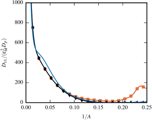
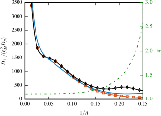
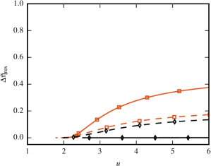
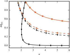
Figure 1: Radial dependence of superbanana plateau $D_{11}$ in the RMP case for Mach number $M_{t}=0.036$ (left) and $-0.036$ (right). Comparison of Hamiltonian approach (NEO-RT) to analytical formula by Shaing Shaing et al. (2009b) (solid line). Results with ($\diamond$) and without magnetic shear ($\square$) in the magnetic drift frequency (38). A safety factor profile (dash-dotted) is shown on the second axis of the upper right plot. The lower plots show resonance lines ranging from deeply trapped ($\Delta\bar{\eta}=0$) to trapped passing boundary ($\Delta\bar{\eta}=1$) at flux surfaces of aspect ratio $A=5$ (solid) and $A=10$ (dashed).

Fig. 1 shows the radial dependence of the transport coefficient $D_{11}$ in the superbanana plateau regime for the RMP-like perturbation for both positive and negative radial electric field. For this benchmarking case the relation between toroidal precession frequencies due to the ${\bf E}\times{\bf B}$ drift, $\Omega_{tE}$, and due to the magnetic drift $\Omega_{tB}$, has been fixed by setting the reference toroidal magnetic drift frequency $\Omega^{\rm ref}_{tB}\equiv cT_{\alpha}/(e_{\alpha}\psi^{a}_{\rm tor})$ (not the actual $\Omega_{tB}$) equal to $\Omega_{tE}$. Additional curves are shown for calculations where the magnetic shear term ($dq/dr$) in Eq. (38) has been neglected. The results are compared to the analytical formula for the large aspect ratio limit by Shaing Shaing et al. (2009b). Resonance lines in velocity space are plotted below the radial profiles for a flux surface relatively close to the axis ($A=10$) and one further outwards ($A=5$). Here $\Delta\bar{\eta}=(\eta-\eta_{\mathrm{tp}})/(\eta_{\mathrm{dt}}-\eta_{\mathrm{tp}})$ is the distance to the trapped passing boundary $\eta_{\mathrm{tp}}$ normalized to the trapped region between trapped-passing boundary $\eta_{\mathrm{tp}}$ and deeply trapped $\eta_{\mathrm{dt}}$. For flux surfaces with $A>10$ magnetic shear plays a small role due to the flat safety factor profile in the present field configuration: The diffusion coefficient $D_{11}$ is nearly identical to the result without shear and stays close to the analytical result for the large aspect ratio limit. For aspect ratio $A=10$, the agreement between NEO-2 calculations and large aspect ratio limit of Ref. Shaing et al., 2009b has been demonstrated earlier in Ref. Kasilov et al., 2014. At larger radii, where the q profile becomes steep, a significant deviation between the cases with and without magnetic shear term is visible. This can be explained by the strong shift of the resonance lines due to the shear term in the rotation frequency $\Omega_{tB}$ that is visible in lower plots. For both signs of the electric field, the resonant $\eta_{\rm res}$ is closer to the trapped passing boundary when shear is included.

In Figs. 2-3 the radial electric field dependence of non-ambipolar transport induced by drift-orbit resonances with magnetic drift neglected ($\Omega_{tB}$ set to zero) is pictured. Here, several canonical modes $m_{2}$ contribute for both, trapped and passing particles.

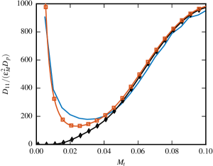
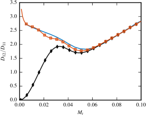
Figure 2: Drift-orbit resonances with neglected magnetic drift: Mach number dependence of $D_{11}$ (left) and the ratio $D_{12}/D_{11}$ (right) for an RMP-like perturbation at $A=10$. Comparison of Hamiltonian approach ($\diamond$), sum of Hamiltonian results and $\nu-\sqrt{\nu}$ regime by Shaing Shaing et al. (2010) ($\square$), and results from NEO-2 at collisionality $\nu^{\star}=3\cdot 10^{-4}$ (solid line).

In Fig. 2 the Mach number dependence of transport coefficient $D_{11}$ and the ratio $D_{12}/D_{11}$ is plotted for this regime for an RMP-like perturbation ($n=3$). NEO-2 calculations shown for the comparison have been performed at rather low collisionality (see the caption) characterized by the parameter $\nu^{\ast}=2\nu qR/v_{T}$ where $\nu$ is the collision frequency. In addition, also the curves with the sum of diffusion coefficients in the collisional $\nu-\sqrt{\nu}$ regime from the joint formula of Shaing Shaing et al. (2010) and resonant contributions from the Hamiltonian approach are shown.

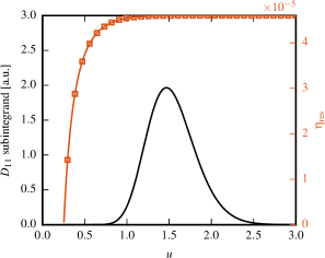
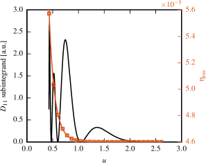
Figure 3: Drift-orbit resonances, RMP at $A=10$ with $M_{t}=0.028$. Dependence of the subintegrands in Eq. (53) on the normalized velocity $u$ for the dominant mode (solid line) of passing (left, $m_{2}=-3$) and trapped particles (right, $m_{2}=-1$) and resonance lines for these modes ($\square$, right axis). Significant contributions are visible where the resonance is close to the trapped passing boundary $\eta_{\rm tp}=4.6\cdot 10^{-5}$.

For $M_{t}<0.02$, in contrast to the superbanana plateau regime, collisionless transport is small compared to collisional effects. Between $M_{t}=0.02$ and $0.04$ the sum of Hamiltonian and $\nu-\sqrt{\nu}$ results for $D_{11}$ is clearly below NEO-2 values. The reason for this are contributions near the trapped passing boundary, which are illustrated in Fig. 3 at $M_{t}=0.028$. There the integrand in Eq. (53) for the mode $m_{2}$ with the strongest contribution is shown together with the resonance line in velocity space. For $M_{t}>0.04$ there is a close match between the results with slightly lower $D_{11}$ values from NEO-2 due to remaining collisionality effects.

It should be noted that validity of the “collisionless” Hamiltonian model cannot be accessed with the help of a simple Krook model although this model is fully adequate for the present derivations. The details of the collision model are not important as long as the collisional width of the resonant line in velocity space is smaller than the distance from that line to the trapped-passing boundary where the topology of the orbits changes abruptly. This criterion is much more restrictive than the smallness of the collision frequency compared to the bounce frequency suggested by the Krook model. At small Mach numbers where the resonant line approaches the trapped-passing boundary rather closely (see Fig. 3), the applicability of the “collisionless” approach is violated at much lower collisionalities than one could expect from the Krook model, and in that case a collisional boundary layer analysis including the resonant interaction is needed. As one can see from Fig. 2, for such transitional Mach numbers where both, $\nu-\sqrt{\nu}$ regime and resonant regime are important, a simple summation of the separate contributions from these regimes obtained in asymptotical limits cannot reproduce the numerical result, similarly to the observation in Ref. Sun et al., 2010. With increasing Mach numbers, the resonant curve gets more separated from the trapped-passing boundary, and the collisionless analysis becomes sufficient, as it can be seen for higher Mach numbers in Fig. 2.

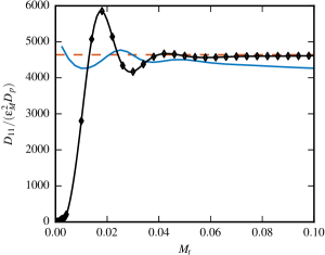
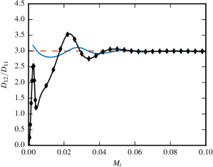
Figure 4: Mach number dependence of transport coefficients of drift-orbit resonances for a toroidal field ripple at $A=10$. Comparison between Hamiltonian approach ($\diamond$), ripple plateau (dashed) and NEO-2 at collisionality $\nu^{\star}=10^{-3}$ (solid line).

Fig. 4 shows the Mach number dependence of $D_{11}$ as well as $D_{12}/D_{11}$ for a toroidal field ripple ($n=18$) together with the analytical ripple plateau value Boozer (1980) and results for finite collisionality from NEO-2. At low Mach numbers $M_{t}<0.01$ collisional effects are again dominant. A resonance peak of passing particles is visible for $D_{12}/D_{11}$ at $M_{t}=2.8\cdot 10^{-3}$. In the intermediate region between $M_{t}=0.01$ and $0.05$ oscillations due to trapped particle resonances are shifted and reduced in the collisional case. For $M_{t}>0.05$ Hamiltonian results converge towards the ripple plateau. A small deviation of NEO-2 values for $D_{11}$, which is of the order of Mach number is caused by the low Mach number approximation used in NEO-2.

Figure 5: Mach number dependence of $D_{11}$ for RMP at $A=5$ with shear term included (left) and neglected (right) in Eq. (38). Total resonant transport ($\diamond$) and contributions by drift-orbit resonances with finite magnetic drift and excluding superbanana plateau ($\square$). Comparison to drift-orbit resonances with $\Omega_{tB}$ set to zero (solid line).

Finally, in Fig. 5 the Mach number dependence of $D_{11}$ for the RMP case is plotted for both, positive and negative Mach numbers for finite toroidal precession frequency due to the magnetic drift $\Omega_{tB}$. To set the scaling with respect to $\Omega_{tE}$, the reference magnetic drift frequency defined above is fixed by $R\Omega^{\rm ref}_{tB}/v_{T}=3.6\cdot 10^{-2}$. In this case all resonance types contribute to transport coefficients. Due to the finite magnetic drift, the Mach number dependence is not symmetric anymore. If shear is neglected in Eq. (38), the superbanana plateau is centered around slightly negative values of the electric field, and magnetic drift induces some deviation from the idealized case without magnetic drift. In the case with included shear superbanana plateau, contributions for positive Mach numbers vanish and a large deviation from the case without magnetic drift is visible also for drift-orbit resonances.

VI Conclusion

In this article, a method for the calculation of the toroidal torque in low-collisional resonant transport regimes due to non-axisymmetric perturbations in tokamaks based on a quasilinear Hamiltonian approach has been presented. This approach leads to a unified description of all those regimes including superbanana plateau and drift-orbit resonances without simplifications of the device geometry. Magnetic drift effects including non-local magnetic shear contributions are consistently taken into account. An efficient numerical treatment is possible by pre-computation of frequencies appearing in the resonance condition.

The analytical expressions for the transport coefficients obtained within the Hamiltonian formalism agree with the corresponding expressions obtained earlier for particular resonant regimes within the validity domains of those results. In particular, the agreement with formulas for the superbanana plateau regime, which have been updated recently for a general tokamak geometry in Ref. Shaing, 2015, is exact. Minor inconsistencies in the treatment of passing particles have been found (see section IV) in comparison to the analytical formulas for bounce-transit resonances of Ref. Shaing et al., 2009a. In addition, it has been demonstrated that momentum conservation of the collision operator plays a minor role in resonant regimes in general as long as the toroidal rotation is sub-sonic.

Results from the newly developed code NEO-RT based on the presented Hamiltonian approach agree well with the results from the NEO-2 code at relatively high Mach numbers where finite collisionality effects are small ($M_{t}>0.04$ in the examples here). At these Mach numbers, both approaches also reproduce the analytical result for the ripple plateau regime Boozer (1980) well. At intermediate Mach numbers $0.02<M_{t}<0.04$ which correspond to the transition between the $\nu-\sqrt{\nu}$ regime and resonant diffusion regime, the combined torque of $\nu-\sqrt{\nu}$ regime and resonant diffusion regime does not reach the numerical values calculated by NEO-2 even at very low collisionalities due to the contribution of the resonant phase space region very close to the trapped-passing boundary. Collisional boundary layer analysis is required in addition to obtain more accurate results in these regions.

Within the Hamiltonian approach, which is non-local by its nature, i.e. it does not use truncated “local” orbits which stay on magnetic flux surfaces, an additional term describing the influence of magnetic shear that is absent in the standard local neoclassical ansatz naturally arises in the resonance condition. This term significantly increases the asymmetry of the superbanana plateau resonance with respect to the toroidal Mach numbers of ${\bf E}\times{\bf B}$ rotation and may even eliminate this resonance for a given Mach number sign (at positive Mach numbers in the examples here). This shear term has been included into analytical treatment recently Shaing (2015) but was absent in earlier approximate formulas Shaing et al. (2009b, 2010). This could be a possible reason for the discrepancy with the non-local $\delta f$ Monte Carlo approach observed in Ref. Satake et al., 2011.

It should be noted that term “non-local transport ansatz” is used here with respect to the orbits employed in the computation of the perturbation of the distribution function, and it should not be confused with the nonlocal transport in the case where the orbit width is comparable to the radial scale of the parameter profiles and where the transport equations cannot be reduced to partial differential equations. In the sense used here, the shear term appears due to a radial displacement of the guiding center, what is a nonlocal effect. Namely, due to variation of the safety factor with radius, the toroidal connection length between the banana tips of the trapped particle is different at the outer and the inner sides of the flux surface containing these tips. Since particles with positive and negative parallel (and, respectively, toroidal) velocity signs are displaced from this surface in different directions, the sum of the toroidal displacements over the full banana orbit is not balanced to zero, what results in an overall toroidal drift proportional to the shear parameter. This effect cannot be described by the local ansatz in an arbitrary coordinate system but still can be retained within the local ansatz in the field aligned coordinates as the ones used in Ref. Shaing, 2015. This ambiguity in the description of the magnetic drift within the local ansatz Smith results from the fact that setting to zero one of the velocity vector components which are not invariant under a coordinate transformation destroys the covariance of equations of motion during such transformations.

Magnetic shear can also have a strong influence on drift-orbit (bounce and bounce-transit) resonances. A comparison between the results in this regime with neglected magnetic drift and results including magnetic drift shows a strong discrepancy, especially if magnetic shear is considered. Therefore, for an accurate evaluation of NTV torque in low-collisional resonant transport regimes it is necessary to consider magnetic drift including magnetic shear in the resonance condition. This is especially important for modern tokamaks with poloidal divertors where magnetic shear is high at the plasma edge where the main part of the NTV torque is produced.

It should be noted that benchmarking with NEO-2 performed in this work resulted in improvement of the analytical quasilinear approach Kasilov et al. (2014) used in NEO-2 as well as in the numerical treatment. In particular, the use of compactly supported basis functions Kernbichler et al. (2016) for the discretization of the energy dependence of the distribution function instead of global Laguerre polynomials used in earlier NEO-2 versions allowed to obtain correct results also at high Mach numbers with rather low collisionality where the global basis resulted in artificial oscillations of the diffusion coefficients with Mach number. In addition, the standard local neoclassical approach used in Ref. Kasilov et al., 2014 for the derivation of quasilinear equations has been generalized to a non-local approach where the effect of magnetic shear is treated appropriately. Details of the derivation will be published in a separate paper. NEO-2 results for NTV in an ASDEX Upgrade equilibrium from both, local and non-local approach are shown and compared in Ref. Martitsch et al., 2016.