Neutrino, $\gamma$-ray and cosmic ray fluxes from the core of the
closest radio galaxies

Abstract

The closest radio galaxies; Centaurus A, M87 and NGC 1275, have been detected from radio wavelengths to TeV $\gamma$-rays, and also studied as high-energy neutrino and ultra-high-energy cosmic ray potential emitters. Their spectral energy distributions show a double-peak feature, which is explained by synchrotron self-Compton model. However, TeV $\gamma$-ray measured spectra could suggest that very-high-energy $\gamma$-rays might have a hadronic origin. We introduce a lepto-hadronic model to describe the broadband spectral energy distribution; from radio to sub GeV photons as synchrotron self-Compton emission and TeV $\gamma$-ray photons as neutral pion decay resulting from p$\gamma$ interactions occurring close to the core. These photo-hadronic interactions take place when Fermi-accelerated protons interact with the seed photons around synchrotron self-Compton peaks. Obtaining a good description of the TeV $\gamma$-ray fluxes, firstly, we compute neutrino fluxes and events expected in IceCube detector and secondly, we estimate ultra-high-energy cosmic ray fluxes and event rate expected in Telescope Array, Pierre Auger and HiRes observatories. Within this scenario we show that the expected high-energy neutrinos cannot explain the astrophysical flux observed by IceCube, and the connection with ultra-high-energy cosmic rays observed by Auger experiment around Centaurus A, might be possible only considering a heavy nuclei composition in the observed events.

1. Introduction

Radio galaxies (RGs) are radio loud active galaxy nuclei (AGN) exhibiting clear structure of a compact central source, large-scale jets and lobes. These sources are also of interest due to the close proximity to the earth affording us an excellent opportunity for studying the physics of relativistic outflows. They have been widely studied from radio wavelengths to MeV-GeV $\gamma$-rays and recently at very-high-energy (VHE) by Imagine Atmospheric Cherenkov Telescope (IACT). RGs are generally described by the standard non-thermal synchrotron self-Compton (SSC) model (Abdo & et al., 2010; Fraija et al., 2012; Tavecchio et al., 1998). In SSC framework, low-energy emission; radio through optical, originates from synchrotron radiation while HE photons; X-rays through $\gamma$-rays, come from inverse Compton scattering emission. However, this model with only one population of electrons, predicts a spectral energy distribution (SED) that can be hardly extended up to higher energies than a few GeVs (Georganopoulos et al., 2005; Lenain et al., 2008). In addition, some authors have suggested that the emission in the GeV - TeV energy range may have origins in different physical processes (Brown & Adams, 2011; Georganopoulos et al., 2005).
The Telescope Array (TA) experiment, located in Millard Country (Utah), was designed to study ultra-high-energy cosmic rays (UHECRs) with energies above 57 EeV (Abu-Zayyad & et al., 2012). TA observatory, with a field of view covering the sky region above -10^∘ of declination, detected a cluster of 72 UHECRs events centered at R. A.=146^∘.7, Dec.=43${}^{\circ}.2$. It had a Li-Ma statistical significance of 5.1$\sigma$ within 5 years of data taking (Abbasi & The Telescope Array Collaboration, 2014). The Pierre Auger observatory (PAO), located in the Mendoza Province of Argentina, was designed to determine the arrival directions and energies of UHECRs using four fluorescence telescope arrays and the High Resolution Fly’s eye (HiRes) experiment, located in the west-central Utah desert, consisted of two detectors that observed cosmic ray showers via the fluorescence light. PAO studying the composition of the high-energy showers found that the distribution of their properties was located in somewhere between pure proton (p) and pure iron (Fe) at 57 EeV(Yamamoto, 2008; Pierre Auger Collaboration & et al., 2008; Unger et al., 2007), although the latest results favored a heavy nuclear composition (Abraham et al., 2010). By contrast, HiRes data were consistent with a dominant proton composition at this energy range (Unger et al., 2007; Engel, 2008). PAO detected 27 UHECRs, with two of them associated with Centaurus A (Cen A), being reconstructed inside a circle centered at the position of this FR I with a aperture of 3.1^∘.
The IceCube detector located at the South Pole was designed to record the interactions of neutrinos. Encompassing a cubic kilometer of ice and almost four years of data taking (from 2010 to 2014), the IceCube telescope reported with the High-Energy Starting Events (HESE) catalog a sample of 54 extraterrestrial neutrino events in the TeV - PeV energy range. Arrival directions of these events are compatible with an isotropic distribution. The neutrino flux is compatible with a high component due to extragalactic origin (Ahlers & Murase, 2014; Gaggero et al., 2015). For instance, gamma-ray bursts (Murase & Ioka, 2013; Razzaque, 2013; Fraija, 2014c; Liu & Wang, 2013; Tamborra & Ando, 2015; Petropoulou et al., 2014a; Fraija, 2016) and AGN (Dermer et al. (2014); Stecker (2013); Petropoulou et al. (2015); Padovani et al. (2015); Marinelli et al. (2014); Fraija (2015); Fraija & Marinelli (2015)), etc.
Hadronic processes producing VHE neutrinos and photons through the acceleration of cosmic rays in AGNs have been explored by many authors (Atoyan & Dermer, 2001; Becker, 2008; Kalashev et al., 2014; Mücke & Protheroe, 2001; Cuoco & Hannestad, 2008; Dermer et al., 2009; Tavecchio & Ghisellini, 2015; Kimura et al., 2015; Hardcastle et al., 2007, 2003). In particular, GeV-TeV $\gamma$-ray fluxes interpreted as pion decay products from photo-hadronic interactions occurring close to the core of RGs have been also discussed for different sources (Sahu et al., 2012; Fraija et al., 2012; Khiali et al., 2015; Khiali & de Gouveia Dal Pino, 2016; Fraija, 2014b; Petropoulou et al., 2014b; Fraija et al., 2015).
In this work we introduce a leptonic and hadronic model to describe the broadband SED of the closest RGs. For the leptonic model, we present the SSC model to explain the SED up to dozens of GeV and for the hadronic model, we propose that the proton-photon (p$\gamma$) interactions occurring close to the core could describe the $\gamma$-ray spectrum at the GeV - TeV energy range. Correlating the TeV $\gamma$-ray, UHECR and neutrino spectra through p$\gamma$ interactions, we estimate their fluxes and number of events expected in PAO, TA and HiRes experiments and IceCube telescope, respectively. For this correlation, we have assumed that the proton spectrum is extended through a simple power law up to UHEs.

2. The closest RGs: Cen A, M87 and NGC1275

In this section, we are going to present a brief description of the three RGs studied in this work and the set of data used in our analysis.

2.1. Cen A

Cen A, at a distance of d${}_{z}\simeq 3.8$ Mpc (z=0.00183), has been one of the best studied radio galaxies. It is characterized by having an off-axis jet estimated in $\sim 15^{\circ}-80^{\circ}$ (see, e.g. Horiuchi et al., 2006, and reference therein) and two giant radio lobes. Cen A has been imaged in radio wavelengths, optical bands (Winkler & White, 1975; Mushotzky et al., 1976; Bowyer et al., 1970; Baity & et al., 1981), X-rays, sub-GeV$\gamma$-rays and VHE $\gamma$-rays (Hardcastle et al., 2003; Sreekumar et al., 1999; Aharonian & et al., 2009; Abdo & et al., 2010; Steinle et al., 1998; Abdo & et al., 2010; Sahakyan et al., 2013). This radio galaxy was observed during a period of 10 months by the Large Area Telescope (LAT) on board the Fermi. The sub-GeV $\gamma$-ray flux collected was described with a power law (F$\propto E^{-\alpha}$ with $\alpha=2.67\pm 0.10_{\rm stat}\pm 0.08_{\rm sys}$; Abdo & et al. (2010)). In addition, Cen A was also detected for more than 120 hr by the High Energy Stereoscopic System (HESS) (Aharonian & et al., 2005, 2009). The observed spectrum ($>$ 250 GeV) was fitted using a simple power law with a spectral index of 2.7$\pm\,0.5_{\rm stat}\pm 0.2_{\rm sys}$ and an apparent luminosity of $\simeq 2.6\times 10^{39}$ erg s^-1. No significant flux variability was detected.

2.2. M87

M87, at a distance of d${}_{z}\simeq 16$ Mpc (z=0.0043), is located in the Virgo cluster of galaxies and hosts a central black hole (BH) of $(3.2\pm 0.9)\times 10^{9}$ solar masses (Bicknell & Begelman, 1996). The jet, inclined at an angle of $\sim$ 15^∘ - 20^∘ relative to the observe’s line of sight, has been imaged in its base down to $\sim$0.01 pc resolution (Junor et al., 1999; Ly et al., 2007). As one of the nearest radio galaxies to us, M87 is amongst the best-studied of its source class. It has been detected from radio wavelengths to VHE $\gamma$ rays. Above 100 MeV, M87 has been detected by LAT-Fermi (Abdo & et al., 2009b), HESS, MAGIC and the Very Energetic Radiation Imaging Telescope Array System (VERITAS) telescopes (Abramowski et al., 2012; Acciari & et al., 2009; Aliu et al., 2012). In 2004, the HESS telescope detected the active galaxy M87 in its historical minimum. The TeV flux measurement was well fitted with a simple power law. The differential energy spectrum was $(2.43\pm 0.75)\times 10^{-13}\,\,{\rm TeV^{-1}\,cm^{-2}\,s^{-1}}$ with a photon index of $2.62\pm 0.35$ (Aharonian et al., 2006). No indications for short-term variability were found.

2.3. NGC1275

NGC 1275, also known as Perseus A and 3C 84, is an elliptical/radio galaxy located at the center of the Perseus cluster at d${}_{z}\simeq 76$ Mpc ($z=0.0179$). This source has a strong, compact nucleus which has been studied in detail with Very Long Baseline Interferometry (VLBI)(Vermeulen et al., 1994; Taylor et al., 2006; Walker et al., 2000; Asada et al., 2006) and Array (VLBA) (Nagai et al., 2014). These observations reveal a compact core and a bowshock-like souther jet component moving steadily outwards at 0.3 mas/year (Kellermann et al., 2004; Lister et al., 2009). The norther counter jet is also detected, though it is much less prominent due to Doppler dimming, as well as to free-free absorption due an intervening disk. Walker, Romney and Berson (1994) derive from these observations that the jet has an intrinsic velocity of $0.3c-0.5c$ oriented at an angle $\approx$ 10^∘ - 35^∘ to the line of sight. Polarization has recently been detected in the southern jet (Taylor et al., 2006), suggesting increasingly strong interactions of the jet with the surrounding environment.
Due to its brightness and proximity, this source has been detected from radio to TeV $\gamma$-ray bands (Abdo & et al., 2009a). This radio galaxy was observed at energies above 100 MeV by Fermi-LAT from 2008 August 4 to 2008 December 5. The average flux and photon index measured, which remained relatively constant during the observing period were $(2.10\pm 0.23)\times 10^{-7}\,{\rm ph\,cm^{-2}\,s^{-1}}$ and $2.17\pm 0.05$, respectively. This source has been detected by MAGIC telescope with a statistical significance of $6.6\,\sigma$ above 100 GeV in 46 hr of stereo observations carried out between August 2010 and February 2011. The measured differential energy spectrum between 70 GeV and 500 GeV was described by a power law with a steep spectral index of $-4.1\pm 0.7_{stat}\pm 0.3_{\rm sys}$, and an average flux of $(1.3\pm 0.2_{stat}\pm 0.3_{\rm sys})\times 10^{-11}\,{\rm cm^{-2}\,s^{-1}}$ (Aleksić & et al., 2012). The light curve ($>$ 100 GeV) did not show hints of variability on a month time scale.

3. Theoretical Model

We propose that the broadband SED of RGs can be described as the superposition of SSC emission and $\pi^{0}$ decay product resulting from p$\gamma$ interactions.

3.1. Leptonic Model

Fermi-accelerated electrons are injected in an emitting region with radius $r_{d}$ which moves at ultra-relativistic velocities with Doppler factor $\delta_{D}$. Relativistic electrons are confined in the emitting region by a magnetic field, therefore it is expected non-thermal photons by synchrotron and Compton scattering radiation.

3.1.1 Synchrotron radiation

The electron population is described by a broken power-law given by (Longair, 1994)

$$N_{e}(\gamma_{e})=N_{0,e}\cases{\gamma_{e}^{-\alpha_{e}}&$\gamma_{\rm e,min}<\gamma_{e}<\gamma_{\rm e,c}$,\cr\gamma_{e,c}\gamma_{e}^{-(\alpha_{e}+1)}&$\gamma_{\rm e,c}\leq\gamma_{e}<\gamma_{\rm e,max}$,\cr}$$ (1)

where $N_{0,e}$ is the proportionality electron constant, $\alpha_{e}$ is the spectral power index of the electron population and $\gamma_{e,i}$ are the electron Lorentz factors. The index $i$ is min, c or max for minimum, cooling and maximum, respectively. By considering that a fraction of total energy density is given to accelerate electrons $U_{e}=m_{e}\int\gamma_{e}N_{e}(\gamma_{e})d\gamma_{e}$, then the minimum electron Lorentz factor and the electron luminosity can be written as

$$\gamma_{\rm e,min} = \frac{(\alpha_{e}-2)}{m_{e}(\alpha_{e}-1)}\,\frac{U_{e}}{N_{e}}\,,$$ (2)

and

$$L_{e}=4\pi\,\delta^{2}_{D}\,r^{2}_{d}\,U_{e}\,,$$ (3)

respectively, where $m_{e}$ is the electron mass. The electron distribution in the emitting region permeated by a magnetic field $B=\sqrt{8\pi\,U_{B}}$ cools down following the cooling synchrotron time scale $t^{\prime}_{c}=\frac{3m_{e}}{4\sigma_{T}}\,\,U^{-1}_{B}\,\gamma^{-1}_{e}$, with $\sigma_{T}=6.65\times 10^{-25}\,{\rm cm^{2}}$ the Compton cross section. Comparing the synchrotron time scale with the dynamic scale $t^{\prime}_{d}\simeq r_{d}/\delta_{D}$, we get that the cooling Lorentz factor is

$$\gamma_{\rm e,c}=\frac{3\,m_{e}}{4\,\sigma_{T}}\,(1+Y)^{-1}\,\delta_{D}\,U_{B}^{-1}\,r_{d}^{-1}\,,$$ (4)

where the Compton parameter is

$$Y\equiv\frac{L_{\rm\gamma,IC}}{L_{\rm syn}}=\frac{U_{\rm rad}}{U_{B}}=\frac{U_{\rm syn}}{U_{B}}=\frac{\eta\,U_{e}}{(1+Y)\,U_{B}}\,.$$ (5)

Here, $L_{\rm\gamma,IC}$ is the observed luminosity around the second SSC peak, $U_{\rm syn}$ and $U_{B}$ are the energy density of synchrotron radiation and magnetic field, respectively. Solving equation (5), the two interesting limits are

$$Y=\cases{\frac{\eta\,U_{e}}{U_{B}}\,,&if $\frac{\eta\,U_{e}}{U_{B}}\ll 1$ ,\cr\left(\frac{\eta\,U_{e}}{U_{B}}\right)^{1/2}\,,&if $\frac{\eta\,U_{e}}{U_{B}}\gg 1$,\cr}$$ (6)

with $\eta=(\gamma_{\rm e,c}/\gamma_{\rm e,min})^{2-\alpha_{e}}$ given for slow cooling and $\eta=1$ for fast cooling (Sari & Esin, 2001). By considering that acceleration time scale $t^{\prime}_{acc}\simeq\sqrt{\frac{\pi}{2}}m_{e}/q_{e}\,U^{-1/2}_{B}\,\gamma_{e}$ and cooling time scale are similar, it is possible to write the maximum electron Lorentz factor as

$$\gamma_{\rm e,max} = \biggl{(}\frac{9\,q_{e}^{2}}{8\pi\,\sigma_{T}^{2}}\biggr{)}^{1/4}\,U_{B}^{-1/4}\,,$$ (7)

where $q_{e}$ is the electric charge. Taking into account the synchrotron emission ${\small\epsilon_{\gamma}(\gamma_{e,i})=\sqrt{\frac{8\pi q_{e}^{2}}{m_{e}^{2}}}\,\delta_{D}\,U_{B}^{1/2}\,\gamma^{2}_{e,i}}$ and eqs. (2), (4) and (7), the synchrotron break energies are

$$\epsilon^{\rm syn}_{\rm\gamma,m} = \frac{\sqrt{8\pi}\,q_{e}}{m_{e}}\,\delta_{D}\,U_{B}^{1/2}\,\gamma^{2}_{\rm e,min}$$ (8)

$$\epsilon^{\rm syn}_{\rm\gamma,c} = \frac{9\sqrt{2\pi}\,q_{e}\,m_{e}}{8\,\sigma_{T}^{2}}\,(1+Y)^{-2}\,\delta_{D}^{3}\,U_{B}^{-3/2}\,r_{d}^{-2}$$ (9)

$$\epsilon^{\rm syn}_{\rm\gamma,max} = \frac{3\,q_{e}^{2}}{m_{e}\,\sigma_{T}}\,\delta_{D}\,.$$ (10)

The synchrotron spectrum is computed through the electron distribution (eq. 1) rather than synchrotron radiation of a single electron. Therefore, the photon energy radiated in the range $\epsilon_{\gamma}$ to $\epsilon_{\gamma}+d\epsilon_{\gamma}$ is given by electrons between $E_{e}$ and $E_{e}+dE_{e}$; then we can estimate the photon spectrum through emissivity $\epsilon_{\gamma}N_{\gamma}(\epsilon_{\gamma})d\epsilon_{\gamma}=(-dE_{e}/dt)\,N_{e}(E_{e})dE_{e}$. Following Longair (1994) and Rybicki & Lightman (1986), one can show that if electron distribution has spectral indexes $\alpha_{e}$ and $(\alpha_{e}-1)$, then the photon distribution has spectral indexes $(\alpha_{e}-1)/2$ and $\alpha_{e}/2$, respectively. The observed synchrotron spectrum can be written as

$$\left[\epsilon^{2}_{\gamma}N(\epsilon_{\gamma})\right]_{\rm\gamma,syn}=A_{\rm\gamma,syn}\cases{(\frac{\epsilon_{\gamma}}{\epsilon^{\rm syn}_{\rm\gamma,m}})^{\frac{4}{3}}&$\epsilon_{\gamma}<\epsilon^{\rm syn}_{\rm\gamma,m}$,\cr(\frac{\epsilon_{\gamma}}{\epsilon^{\rm syn}_{\rm\gamma,m}})^{-\frac{\alpha_{e}-3}{2}}&$\epsilon^{\rm syn}_{\rm\gamma,m}<\epsilon_{\gamma}<\epsilon^{\rm syn}_{\rm\gamma,c}$,\cr(\frac{\epsilon^{\rm syn}_{\rm\gamma,c}}{\epsilon^{\rm syn}_{\rm\gamma,m}})^{-\frac{\alpha_{e}-3}{2}}(\frac{\epsilon_{\gamma}}{\epsilon_{\rm\gamma,c}})^{-\frac{\alpha_{e}-2}{2}},&$\epsilon^{\rm syn}_{\rm\gamma,c}<\epsilon_{\gamma}<\epsilon^{\rm syn}_{\rm\gamma,max}$\,,\cr}$$ (11)

where $A_{\rm\gamma,syn}$ is the proportionality constant of synchrotron spectrum. This constant can be estimated through the total number of radiating electrons in the volume of emitting region, ${\small n_{e}=N_{e}/V=4\pi N_{e}\,r_{d}^{3}/3}$, the maximum radiation power ${\small P_{\rm\nu,max}\simeq\frac{dE_{e}/dt}{\epsilon_{\gamma}(\gamma_{e})}}$ and the distance d_z from the source. Therefore, the proportionality constant can be written as

$$A_{\rm\gamma,syn} = \frac{P_{\rm\nu,max}n_{e}}{4\pi d_{z}^{2}}\,\epsilon^{\rm syn}_{\rm\gamma,m}$$ (12)

$$= \frac{4\,\sigma_{T}}{9}\,d^{2}_{z}\,\delta^{3}_{D}\,U_{B}\,r_{d}^{3}\,N_{e}\,\gamma^{2}_{\rm e,min}\,.$$ (13)

3.1.2 Compton scattering emission

Fermi-accelerated electrons in the emitting region can upscatter synchrotron photons up to higher energies as

$$\epsilon^{\rm ssc}_{\gamma,{\rm(m,c,max)}}\simeq\gamma^{2}_{e,{\rm(min,c,max)}}\epsilon^{\rm syn}_{\gamma,{\rm(m,c,max)}}\,.$$ (14)

From the electron Lorentz factors (eqs. 2, 4, 7) and the synchrotron break energies (eq. 8), we get that the Compton scattering break energies are given in the form

$$\epsilon^{\rm ssc}_{\rm\gamma,m} = \frac{\sqrt{8\pi}\,q_{e}}{m_{e}}\,\delta_{D}\,U_{B}^{1/2}\,\gamma^{4}_{\rm e,min},$$ (15)

$$\epsilon^{\rm ssc}_{\rm\gamma,c} = \frac{81\sqrt{2\pi}\,q_{e}\,m_{e}^{3}}{128\,\sigma_{T}^{4}}\,(1+Y)^{-4}\,\delta_{D}^{5}\,U_{B}^{-7/2}\,r_{d}^{-4},$$ (16)

$$\epsilon^{\rm ssc}_{\rm\gamma,max} = \frac{9\,q_{e}^{3}}{2\sqrt{2\pi}\,m_{e}\,\sigma^{2}_{T}}\,\delta_{D}\,U_{B}^{-1/2}\,.$$ (17)

The Compton scattering spectrum obtained as a function of the synchrotron spectrum (eq. 11) is

$$\left[\epsilon^{2}_{\gamma}N(\epsilon_{\gamma})\right]_{\rm\gamma,ssc}=A_{\rm\gamma,ssc}\cases{(\frac{\epsilon_{\gamma}}{\epsilon^{\rm ssc}_{\rm\gamma,m}})^{\frac{4}{3}}&$\epsilon_{\gamma}<\epsilon^{ssc}_{\gamma,m}$,\cr(\frac{\epsilon_{\gamma}}{\epsilon^{\rm ssc}_{\rm\gamma,m}})^{-\frac{\alpha_{e}-3}{2}}&$\epsilon^{\rm ssc}_{\rm\gamma,m}<\epsilon_{\gamma}<\epsilon^{\rm ssc}_{\rm\gamma,c}$,\cr(\frac{\epsilon^{\rm ssc}_{\rm\gamma,c}}{\epsilon^{ssc}_{\gamma,m}})^{-\frac{\alpha_{e}-3}{2}}(\frac{\epsilon_{\gamma}}{\epsilon^{ssc}_{\gamma,c}})^{-\frac{\alpha_{e}-2}{2}},&$\epsilon^{\rm ssc}_{\rm\gamma,c}<\epsilon_{\gamma}<\epsilon^{\rm ssc}_{\rm\gamma,max}$}$$ (18)

where $A_{\rm\gamma,ssc}=Y\,[\epsilon^{2}_{\gamma}N_{\gamma}(\epsilon_{\gamma})]_{\rm max}^{\rm syn}$ is the proportionality constant of Compton scattering spectrum.

3.2. Hadronic Model

RGs have been proposed as a powerful accelerator of charged particles through the Fermi acceleration mechanism or/and magnetic reconnection (Khiali et al., 2015). We consider a proton population described as a simple power law given by

$$\left(\frac{dN}{dE}\right)_{p}=A_{p}\,E_{p}^{-\alpha_{p}}\,,$$ (20)

with $A_{p}$ the proportionality constant and $\alpha_{p}$ the spectral power index of the proton population. From eqs. (20) we can compute that the proton density can be written as

$$U_{p}=\frac{L_{p}}{4\pi\,\delta^{2}_{D}\,r^{2}_{d}}\,,$$ (21)

with the proton luminosity given by

$$L_{p}=4\,\pi\,d^{2}_{z}A_{p}\,\int\,E_{p}\,E_{p}^{-\alpha_{p}}dE_{p}\,.$$ (22)

Fermi-accelerated protons lose their energies by electromagnetic channels and hadronic interactions. Electromagnetic channels such as proton synchrotron radiation and inverse Compton will not be considered here, we will only assume that protons will be cooled down by p$\gamma$ interactions at the emitting region of the inner jet. Charged ($\pi^{+}$) and neutral ($\pi^{0}$) pions are obtained from p$\gamma$ interaction through the following channels

$$p\,\gamma \longrightarrow \Delta^{+}\longrightarrow\left\{\begin{array}[]{lll}p\,\pi^{0}&&\mbox{fraction }2/3,\\ n\,\pi^{+}&&\mbox{fraction }1/3\,.\end{array}\right.$$

After that neutral pion decays into photons, $\pi^{0}\rightarrow\gamma\gamma$, carrying $20\%(\xi_{\pi^{0}}=0.2)$ of the proton’s energy $E_{p}$. The efficiency of the photo-pion production is (Stecker, 1968; Waxman & Bahcall, 1997)

$$f_{\pi^{0}}\simeq\frac{t_{\rm dyn}}{t^{-1}_{\pi^{0}}}=\frac{r_{d}}{2\gamma^{2}_{p}}\int\,d\epsilon\,\sigma_{\pi}(\epsilon)\,\xi_{\pi^{0}}\,\epsilon\int dx\,x^{-2}\,\frac{dn_{\gamma}}{d\epsilon_{\gamma}}(\epsilon_{\gamma}=x)\,,$$ (26)

where $dn_{\gamma}/d\epsilon_{\gamma}$ is the spectrum of seed photons, $\sigma_{\pi}(\epsilon_{\gamma})$ is the cross section of pion production and $\gamma_{p}$ is the proton Lorentz factor. Solving the integrals we obtain

$$f_{\pi^{0}}\simeq\frac{\sigma_{\rm p\gamma}\,\Delta\epsilon_{\rm res}\,\xi_{\pi^{0}}\,L_{\rm\gamma,IC}}{4\pi\,\delta_{D}^{2}\,r_{d}\,\epsilon_{\rm pk,ic}\,\epsilon_{\rm res}}\cases{\left(\frac{\epsilon^{\pi^{0}}_{\gamma}}{\epsilon^{\pi^{0}}_{\gamma,c}}\right)^{\beta_{h}-1}&$\epsilon_{\gamma}<\epsilon^{\pi^{0}}_{\gamma,c}$\cr\left(\frac{\epsilon^{\pi^{0}}_{\gamma}}{\epsilon^{\pi^{0}}_{\gamma,c}}\right)^{\beta_{l}-1}&$\epsilon^{\pi^{0}}_{\gamma,c}<\epsilon_{\gamma}$\,,\cr}$$ (27)

where $\beta_{h}$ and $\beta_{l}$ are the high-energy and low-energy photon index, respectively, ($L_{\rm\gamma,IC}$) is the observed luminosity around the second SSC peak, $\Delta\epsilon_{\rm res}$=0.2 GeV, $\epsilon_{\rm res}\simeq$ 0.3 GeV, $\epsilon_{\rm pk,ic}$ is the energy of the second SSC peak and $\epsilon^{\pi^{0}}_{\gamma,c}$ is the break photon-pion energy given by

$$\epsilon^{\pi^{0}}_{\gamma,c}\simeq 31.87\,{\rm GeV}\,\delta_{D}^{2}\,\left(\frac{\epsilon_{\rm pk,ic}}{{\rm MeV}}\right)^{-1}\,.$$ (28)

It is worth noting that the target photon density and the optical depth can be obtained through the equations

$$n_{\gamma}\simeq\frac{L_{\rm\gamma,IC}}{4\pi r^{2}_{d}\,\epsilon_{\rm pk,ic}}\,,$$ (29)

and

$$\tau_{\gamma}\simeq\frac{L_{\rm\gamma,IC}\,\sigma_{T}}{4\pi r_{d}\,\delta_{D}\epsilon_{\rm pk,ic}}\,.$$ (30)

respectively. Taking into account that photons released in the range $\epsilon_{\gamma}$ to $\epsilon_{\gamma}+d\epsilon_{\gamma}$ by protons in the range $E_{p}$ and $E_{p}+dE_{p}$ are $f_{\pi^{0}}\,E_{p}\,(dN/dE)_{p}\,dE_{p}=\epsilon_{\pi^{0},\gamma}\,(dN/d\epsilon)_{\pi^{0},\gamma}\,d\epsilon_{\pi^{0},\gamma}$, then photo-pion spectrum is given by

$$\left[\epsilon^{2}_{\gamma}N(\epsilon_{\gamma})\right]_{\rm\gamma,\pi^{0}}=A_{\rm p\gamma}\left(\frac{\epsilon^{\pi^{0}}_{\gamma,c}}{\epsilon_{0}}\right)^{-\alpha_{p}+2}\cases{\left(\frac{\epsilon^{\pi^{0}}_{\gamma}}{\epsilon^{\pi^{0}}_{\gamma,c}}\right)^{\beta_{h}+1-\alpha_{p}}&$\epsilon_{\gamma}<\epsilon^{\pi^{0}}_{\gamma,c}$\cr\left(\frac{\epsilon^{\pi^{0}}_{\gamma}}{\epsilon^{\pi^{0}}_{\gamma,c}}\right)^{\beta_{l}+1-\alpha_{p}}&$\epsilon^{\pi^{0}}_{\gamma,c}<\epsilon_{\gamma}$\,,\cr}$$ (31)

where the proportionality constant $A_{\rm p\gamma}$ is in the form

$$A_{\rm p\gamma}=\frac{L_{\rm\gamma,IC}\,\sigma_{\rm p\gamma}\,\Delta\epsilon_{\rm res}\,\epsilon^{2}_{0}\,\left(\frac{2}{\xi_{\pi^{0}}}\right)^{1-\alpha_{p}}}{4\pi\,\delta_{D}^{2}\,r_{d}\,\epsilon_{\rm pk,ic}\,\epsilon_{\rm res}}\,A_{p}\,.$$ (32)

The value of $A_{p}$ is determined through the TeV $\gamma$-ray flux (eq. 32).

4. High energy neutrino expectation

Photo hadronic interactions in the emitting region (see subsection 3.2) also generate neutrinos through the charged pion decay products ($\pi^{\pm}\rightarrow\mu^{\pm}+\nu_{\mu}/\bar{\nu}_{\mu}\rightarrow e^{\pm}+\nu_{\mu}/\bar{\nu}_{\mu}+\bar{\nu}_{\mu}/\nu_{\mu}+\nu_{e}/\bar{\nu}_{e}$). Taking into account the distances of RGs, the neutrino flux ratio (1 : 2 : 0 ) created on the source will arrive on the standard ratio (1 : 1 : 1 ) (Becker, 2008). The neutrino spectrum produced by the photo hadronic interactions is

$$\left[E_{\nu}^{2}N(\epsilon_{\nu})\right]_{\nu}=A_{\nu}\epsilon^{2}_{0}\cases{\left(\frac{E_{\nu}}{\epsilon_{0}}\right)^{\beta_{h}}&$E_{\nu}<E_{\nu,c}$\cr\left(\frac{E_{\nu}}{\epsilon_{0}}\right)^{\beta_{l}+1-\alpha_{\nu}}&$E_{\nu,c}<E_{\nu}$\,,\cr}$$ (33)

where the factor, A_ν, normalized through the TeV $\gamma$-ray flux is (see, Julia Becker Halzen, 2007, and reference therein)

$$A_{\nu}=A_{\rm p\gamma}\,\epsilon_{0}^{-2}\,2^{-\alpha_{p}}\,.$$ (34)

The previous equation was obtained from solving the integral terms $\int\frac{dN_{\nu}}{dE_{\nu}}\,E_{\nu}\,dE_{\nu}=\frac{1}{4}\int\frac{dN_{\gamma}}{dE_{\gamma}}\,E_{\gamma}\,dE_{\gamma}$, considering that the spectral indices for neutrino and that $\gamma$-ray spectra are similar $\alpha_{p}\simeq\alpha_{\nu}$ (Becker, 2008) and each neutrino (photon) bring 5% (10%) of the initial proton energy. The neutrino flux is detected when it interacts inside the instrumented volume. Considering the probability of interaction for a neutrino with energy $E_{\nu}$ in an effective volume ($V_{eff}$) with density ($\rho_{ice}$), the number of expected neutrino events after a period of time $T$ is

$$N_{\rm ev}\approx\,T\rho_{\rm ice}\,N_{A}\,\epsilon_{0}\int_{E_{\rm\nu,th}}V_{\rm eff}(E_{\nu})\sigma_{\rm\nu N}(E_{\nu})\,A_{\nu}\left(\frac{E_{\nu}}{\epsilon_{0}}\right)^{-\alpha_{p}}\,dE_{\nu}\,,$$ (35)

where $N_{A}$ is the Avogadro number, $\sigma_{\nu N}(E_{\nu})$ is the the charged current cross section and $E_{\nu,th}$ is the energy threshold. It is worth noting that the effective volume $V_{eff}$ is obtained for a hypothetical Km³ neutrino telescope through the Monte Carlo simulation.

5. Ultra-high-energy cosmic rays

TeV $\gamma$-ray observations from low-redshift AGN have been proposed as good candidates for studying UHECRs (Murase et al., 2012; Dermer et al., 2009; Razzaque et al., 2012). We consider that the proton spectrum is extended up to UHEs and then calculate the number of events expected in PAO, TA and HiRes experiments.

5.1. Hillas Condition

By considering that super massive BHs have the power to accelerate particles up to UHEs through Fermi processes, protons accelerated in the emitting region are confined by the Hillas condition (Hillas, 1984). Although this requirement is a necessary condition and acceleration of UHECRs in AGN jets (Murase et al., 2012; Razzaque et al., 2012; Jiang et al., 2010), it is far from trivial (see e.g., Lemoine & Waxman (2009) for a more detailed energetic limits). The Hillas criterion is defined as the maximum proton energy achieved in a region with radius $r_{d}$ and magnetic field $B$. It can be written as

$$E_{\rm p,max}\simeq\frac{Zq_{e}}{\phi}\,B\,r_{d}\,\Gamma\,.$$ (36)

Here $Z$ is the atomic number, $\phi\simeq$ 1 is the acceleration efficiency factor and $\Gamma$ is the bulk Lorentz factor given by

$$\Gamma=\frac{1\pm\sqrt{1-(1-\cos^{2}\theta)(1+\delta^{2}_{D}\cos^{2}\theta)}}{\delta_{D}(1-\cos^{2}\theta)}\,,$$ (37)

where $\theta$ is the viewing angle.

5.2. Deflections

The magnetic fields play important roles on cosmic rays. UHECRs traveling from source to Earth are randomly deviated by galactic (B_G) and extragalactic (B_EG) magnetic fields. By considering that magnetic fields are quasi-constant and homogeneous, the deflection angle due to the B_G and B_EG (Stanev, 1997) are

$$\psi_{\rm G}\simeq 3.8^{\circ}\left(\frac{E_{p,th}}{57EeV}\right)^{-1}\int^{L_{G}}_{0}|\frac{dl}{{\rm kpc}}\times\frac{B_{G}}{4\,{\rm\mu G}}|\,,$$ (38)

and

$$\psi_{\rm EG}\simeq 4^{\circ}\left(\frac{E_{p,th}}{57EeV}\right)^{-1}\,\left(\frac{L_{\rm EG}}{100\,{\rm Mpc}}\right)^{1/2}\,\left(\frac{l_{c}}{1\,{\rm Mpc}}\right)^{1/2}\,\left(\frac{B_{\rm EG}}{1\,{\rm nG}}\right)\,,$$ (39)

respectively, where L_G corresponds to the distance of our Galaxy (20 kpc), $l_{c}$ is the coherence length and $E_{\rm p,th}$ is the threshold proton energy. Due to the strength of extragalactic ($B_{\rm EG}\simeq$ 1 nG) and galactic ($B_{\rm G}\simeq$ 4 $\mu$G) magnetic fields, UHECRs are deflected; firstly, $\psi_{\rm EG}\simeq 4^{\circ}$ and after $\psi_{G}\simeq 3.8^{\circ}$, between the true direction to the source and the observed arrival direction, respectively. Estimation of the deflection angles could associate the transient UHECR sources with the HE neutrino and $\gamma$-ray fluxes. Taking into account of extragalactic and galactic magnetic fields, it is reasonable to correlate UHECRs lying within $\sim 5^{\circ}$ of a source.

5.3. Expected number of events

Telescope Array observatory

. Located in Millard Country (Utah), TA experiment was designed to study UHECRs with energies above 57 EeV. With an area of $\sim$ 700 km², it is made of a scintillator surface detector (SD) array and three fluorescence detector (FD) stations (Abu-Zayyad & et al., 2012). The TA exposure is given by $\Xi\,t_{op}\,\omega(\delta_{s})/\Omega$, where $\Xi\,t_{op}=(5)\,7\times 10^{2}\,\rm km^{2}\,yr$, $t_{op}$ is the total operational time (from 2008 May 11 and 2013 May 4), $\omega(\delta_{s})$ is an exposure correction factor for the declination of the source (Sommers, 2001) and $\Omega\simeq\pi$.

Pierre Auger observatory

. The PAO, located in the Mendoza Province of Argentina at latitude $\simeq 36^{\circ}$S, was designed to determine the arrival directions and energies of UHECRs using four fluorescence telescope arrays and 1600 surface detectors spaced 1.5 km apart. The large exposure of its ground array, combined with accurate energy has provided an opportunity to explore the spatial correlation between cosmic rays and their sources in the sky. The PAO exposure is given by $\Xi\,t_{op}\,\omega(\delta_{s})/\Omega_{60}$, where $\Xi\,t_{op}=9\times 10^{3}\,\rm km^{2}\,yr$, $t_{op}$ is the total operational time (from 1 January 2004 until 31 August 2007), $\omega(\delta_{s})$ is an exposure correction factor and $\Omega_{60}\simeq\pi$ is the Auger acceptance solid angle (Pierre Auger Collaboration & et al., 2007, 2008).

The High Resolution Fly’s eye experiment

. The HiRes experiment, located atop two hills 12.6 km apart in the west-central Utah desert, consisted of two detectors that observed cosmic ray showers via the fluorescence light. Both detectors, called HiRes-I and HiRes-II, consisted of 21 and 42 telescopes, respectively, each one composed of a spherical mirror of 3.8 m². The HiRes exposure is (3.2 - 3.4) $\times 10^{3}$ km² year sr. HiRes experiment measured the flux of UHECRs using the stereoscopic air fluorescence technique over a period of nine years (1997 - 2006) (Abbasi et al., 2005; High Resolution Fly’S Eye Collaboration et al., 2009).
The expected number of UHECRs above an energy $E_{p,th}$ yields

$$N_{\rm\tiny UHECR}=({\rm Expos.})\times\,N_{p},$$ (40)

where $N_{p}$ is calculated from the proton spectrum extended up to energies higher than $E_{p,th}$ (eq. 20). The expected number can be written as

$$N_{\rm\tiny UHECR}=\frac{\Xi\,t_{\rm op}\,\omega(\delta_{s})}{(\alpha_{p}-1)\Omega}\,A_{p}\int_{E_{\rm p,th}}E_{p}^{-\alpha_{p}}dE_{p}\,,$$ (41)

where the value of $A_{p}$ is normalized with the TeV $\gamma$-ray fluxes (eq. 32).

6. Results and Discussion

We have presented a lepto-hadronic model to describe the broadband SED of the closest RGs, supposing that electrons and protons are co-accelerated at the emitting region of the jet. In the leptonic model, we have required the SSC model to explain the spectrum up to dozens of GeV and in the hadronic scenario, we have evoked the p$\gamma$ interactions occurring close to the core of the RGs to interpret the TeV $\gamma$-ray fluxes. The SSC model depends basically on magnetic field ($B$), electron density ($N_{e}$), size of emitting region ($r_{d}$) and Doppler factor ($\delta_{D}$). To reproduce the electromagnetic spectrum up to dozens of GeV, we have used an electron distribution described by a broken power law (eq. 1) with the minimum, cooling and maximum Lorentz factors given by eqs. (2), (4), (7), respectively. The minimum Lorentz factor is obtained through electron density and electron energy density, the cooling Lorentz factor is computed through the synchrotron and dynamical time scales, and the maximum Lorentz factor is calculated considering the synchrotron and the acceleration time scales. Considering the break Lorentz factors, the synchrotron and Compton scattering break energies are obtained (eqs. 8 and 15). The synchrotron (eq. 11) and Compton scattering (eq. 18) spectra are estimated through the density and distribution of radiating electrons confined inside emitting region. In the p$\gamma$ interaction model, we have considered Fermi-accelerated protons described by a simple power law (eq. 20) which are accelerated close to the core and furthermore interact with the photon population at the second-peak SED photons. The spectrum generated by this hadronic process (eq. 33) depends on the proton luminosity (through $A_{p}$), the observed luminosity around the second SSC peak ($L_{\rm\gamma,IC}$), the energy of the second SSC peak ($\epsilon_{\rm pk,ic}$), the size of emitting region, the Doppler factor, and the high-energy and low-energy photon index, respectively. The efficiency of the photo-production (eq. 26) is calculated through the photo-pion cooling and dynamical time scales for $\beta_{h}\sim 2$ and $\beta_{l}\sim 1$. Evoking these interactions, we have interpreted naturally the TeV $\gamma$-ray spectra as $\pi^{0}$ decay products.
We have required the data used by the Fermi collaboration for Cen A (Abdo & et al., 2010), M87 (Abdo & et al., 2009b) and NGC1275 (Abdo & et al., 2009a). In the case of NGC1275, the TeV $\gamma$-ray data have been added (Aleksić & et al., 2012). Using the method of Chi-square $\chi^{2}$ minimization as implemented in the ROOT software package (Brun & Rademakers, 1997), we get the break energies, spectral indexes and normalization of the SSC and photo-pion spectrum as reported in Table 1 and Figures 1, 2 and 3 for Cen A , M87 and NGC1275, respectively. For the sake of simplicity, the process was integrated into a python script that called the ROOT routines via the pyroot module. The whole data of the closest RGs were read from a file and written into an array which was then fitted with pyROOT. The fitted data with the PyROOT module and from eqs. (11), (18) and (33) were plotted with a smooth sbezier curve through the gnuplot software . The sbezier option first renders the data monotonic (unique) and then applies the Bezier algorithm.

Table 1. Values obtained after fitting the whole spectrum of the RGs with our lepto-hadronic model.

Parameter	Symbol	Cen A	M87	NGC1275
Leptonic model
$A_{\rm syn,\gamma}\,\,({\rm MeV\,cm^{-2}\,s^{-1}})$	[0]	$(0.25\pm 0.05)\times 10^{-4}$	$(0.66\pm 0.08)\times 10^{-4}$	$(1.25\pm 0.26)\times 10^{-5}$
$\alpha_{e}$	[1]	3.50$\pm$ 0.02	3.21$\pm$ 0.02	2.81$\pm$ 0.05
$\epsilon^{syn}_{\rm\gamma,m}\,\,({\rm eV})$	[2]	$0.046\pm 0.002$	$(2.26\pm 0.25)\times 10^{-2}$	$(1.25\pm 0.05)\times 10^{-2}$
$\epsilon^{syn}_{\rm\gamma,c}\,\,({\rm eV})$	[3]	0.15$\pm$ 0.02	$0.15\pm 0.02$	$0.33\pm 0.02$
$A_{\rm ssc,\gamma}\,\,({\rm MeV\,cm^{-2}\,s^{-1}})$	[4]	$(6.65\pm 0.67)\times 10^{-4}$	$(1.31\pm 0.75)\times 10^{-5}$	$(3.99\pm 0.86)\times 10^{-4}$
$\epsilon^{\rm ssc}_{\rm\gamma,m}\,\,({\rm keV})$	[5]	$67.1\pm 1.51$	$11.2\pm 0.9$	$3.15\pm 0.16$
$\epsilon^{\rm ssc}_{\rm\gamma,c}\,\,({\rm MeV})$	[6]	$0.53\pm 0.02$	$0.41\pm 0.15$	$2.1\pm 0.1$
Hadronic model
$A_{\rm p\gamma}\,\,({\rm MeV\,cm^{-2}\,s^{-1}})$	[7]	$(3.98\pm 0.18)\times 10^{-7}$	$(1.17\pm 0.24)\times 10^{-7}$	$(3.69\pm 0.91)\times 10^{-7}$
$\alpha_{p}$	[8]	2.81$\pm$ 0.05	2.80$\pm$ 0.02	$3.81\pm 0.64$

From eqs. (8), (12), (15) and the values reported in Table 1, we have obtained the values of magnetic field, electron density, size of emitting region and Doppler factor that describe the broadband SED of Cen A, M87 and NGC1275. For this fit, we have considered the effect of the electromagnetic background light (EBL) absorption (Franceschini et al., 2008) and adopted the typical values reported in the literature such as viewing angles, observed luminosities, distances of the closest RGs, minimum Lorentz factors and energy normalizations (Ferrarese et al., 2007; Tonry, 1991; Strauss et al., 1992; Abdo & et al., 2010; Bicknell & Begelman, 1996; Asada et al., 2006; Aharonian & et al., 2009; Aharonian et al., 2006; Aleksić & et al., 2012; Abdo & et al., 2009b, a; Steinle et al., 1998; Ajello et al., 2009). Other quantities such as bulk Lorentz factors, proton and electron luminosities, magnetic field, proton and electron densities, etc, are derived from these parameters. Table 2 shows all the parameter values obtained, used and derived in and from the fit.
The maximum proton Lorentz factors were estimated with the maximum electron Lorentz factors as $\gamma_{p,max}=\frac{m_{p}}{m_{e}}\gamma_{e,max}$ (Petropoulou et al., 2014b). Requiring that electron and proton number densities are similar ($N_{e}\simeq N_{p}$), we have calculated the minimum proton Lorentz factors $\gamma_{p,min}$. These values could increase/decrease considering that proton number density is smaller/higher than the electron number density. For instance, if we assume that ($N_{p}\simeq b\,N_{e}$) with b=10 (0.1) the minimum proton Lorentz factors are $\gamma_{p,min}=9.1\times 10^{3}$ ($1.6\times 10^{6}$), $3.2\times 10^{5}$ ($6.7\times 10^{7}$) and $7.1\times 10^{5}$ ($9.2\times 10^{6}$) for Cen A, M87 and NGC1275, respectively. Due to the fact that the minimum Lorentz factor cannot be determined just assuming the standard scenario of injection and acceleration, we have used the condition that electron and proton number densities are similar. Otherwise, for $\gamma_{p,min}=1$ the proton luminosities becomes $>5\times 10^{47}\,{\rm erg/s}$. Considering the values of magnetic field, electron and proton energy densities, and their rates; $\lambda_{e,B}=\frac{U_{e}}{U_{B}}$ ($\lambda_{p,B}=\frac{U_{p}}{U_{B}}$)= 2.92 (4.90), 24.1 (26.9) and 117.81 (382.56) for Cen A, M87 and NGC1275, respectively, we can see that energy densities could be related through principle of equipartition.

Table 2. Parameters obtained, derived and used of lepton-hadronic model to fit the spectrum of Cen A, M87 and NGC1275.

	Cen A	M87	NGC1275
Obtained quantities
$\delta_{d}$	1.0	2.8	2.2
$B$ (G)	3.6	1.61	2.01
$r_{d}$ (cm)	$5.2\times 10^{15}\,$	$2.1\times 10^{15}\,$	$2.26\times 10^{15}\,$
$N_{e}$ (cm-3)	$1.1\times 10^{3}$	$2.3\times 10^{3}$	$3.11\times 10^{4}$
Used quantities				References
$d_{z}\,\,({\rm Mpc})$	3.7	16	76	(1,2,3)
$\theta$  (degree)	30	17	20	(4,5,6)
$\epsilon_{0}$  (TeV)	1	1	1	(7,8,9)
$\gamma_{\rm e,min}$	$1.2\times 10^{3}$	$0.67\times 10^{3}$	$0.5\times 10^{3}$	(4,10,11)
$L_{\rm\gamma,IC}\,\,{\rm(erg/s)}$	$5\times 10^{42}$	$5\times 10^{42}$	$5\times 10^{42}$	(12, 13)
Derived quatities
$\Gamma$	7.0	6.47	6.29
$f_{\pi^{0}}$	$1.05\times 10^{-6}$	$6.68\times 10^{-8}$	$1.55\times 10^{-8}$
$\tau_{\gamma}$	$7.89\times 10^{-6}$	$1.40\times 10^{-6}$	$2.56\times 10^{-7}$
$\gamma_{e,max}$	$3.64\times 10^{7}$	$3.70\times 10^{7}$	$3.29\times 10^{7}$
$\gamma_{p,min}$	$1.0\times 10^{5}$	$7.0\times 10^{6}$	$2.4\times 10^{6}$
${}^{a}\gamma_{p,max}$	$6.73\times 10^{10}$	$6.76\times 10^{10}$	$6.04\times 10^{10}$
$\epsilon_{\rm pk,ic}\,\,({\rm MeV})$	$0.1$	$0.5$	$3.5$
$\epsilon_{\pi^{0},\gamma,c}\,\,({\rm TeV})$	$0.32$	$0.54$	$0.05$
$U_{B}\,\,{\rm(erg/cm^{3})}$	$0.52$	$0.10$	$0.16$
$U_{e}\,\,{\rm(erg/cm^{3}})$	$1.52$	$2.41$	$28.45$
$U_{p}\,\,{\rm(erg/cm^{3}})$	$2.55$	$2.69$	$61.21$
$L_{p}\,\,{\rm(erg/s)}$	$3.74\times 10^{43}$	$4.89\times 10^{43}$	$2.29\times 10^{44}$
$L_{e}\,\,{\rm(erg/s})$	$1.55\times 10^{43}$	$3.17\times 10^{43}$	$2.27\times 10^{44}$
$E_{\rm p,max}\,\,{\rm(EeV)}$	$40.1$	$6.55$	$7.92$
$N_{\rm\tiny UHECRs}$	$1.52$	$0.41$	$2.63\times 10^{-6}$

Notes.
^a $\gamma_{p,max}=\frac{m_{p}}{m_{e}}\gamma_{e,max}$.
References. (1) Ferrarese et al. (2007) (2) Tonry (1991) (3) Strauss et al. (1992) (4) Abdo & et al. (2010) (5) Bicknell & Begelman (1996) (6) Asada et al. (2006) (7) Aharonian & et al. (2009) (8) Aharonian et al. (2006) (9) Aleksić & et al. (2012) (11) Abdo & et al. (2009b) (10) Abdo & et al. (2009a) (12) Steinle et al. (1998) (13) Ajello et al. (2009).

We plot in a sky-map the 54 neutrino events detected by the IceCube collaboration, the 72 and 27 UHECRs collected by TA and PAO experiments, respectively, and also a circular region of 5^∘ around the closest RGs, as shown in Figure 4. This figure shows that whereas there are not neutrino track events associated to Cen A, M87 and NGC1275, two UHECRs are only enclosed around Cen A.
By assuming that the inner part of the RG jet has the potential to accelerate particles up to UHEs, we can see that protons at the emitting region can achieve maximum energies of 40.1, 6.55 and 7.92 EeV for Cen A, M87 and NGC1275, respectively, as shown in Table 2. Therefore, it is improbable that protons can be accelerated to energies as high as 57 EeV, although it is plausible for heavier accelerated ions. In this case, they can be disintegrated by infrared photons from the core. It is worth noting that any small variation in the strength of magnetic field and/or size of emitting region would allow that protons could achieve a maximum energy of 57 EeV for Cen A. Similarly, supposing that the BH jet has the power also to accelerate particles up to UHEs through Fermi processes, then during flaring intervals (for which the apparent isotropic luminosity can reach $\approx 10^{46}$ erg s^-1 and from the equipartition magnetic field $\epsilon_{B}$) the maximum particle energy of accelerated UHECRs can achieve values as high as $E_{\rm max}\approx 3.0\times 10^{20}\,\frac{Zq_{e}\,\epsilon^{1/2}_{B}}{\phi\,\Gamma}\,\left(\frac{L}{10^{46}\,{\rm erg/s}}\right)^{1/2}\,{\rm eV}$ (Dermer et al., 2009). Describing the TeV gamma-ray spectra through p$\gamma$ interaction and extrapolating the interacting proton spectra up to energies higher than 1 EeV, we plot the UHE proton spectra expected for these three RGs (Cen A, M87 and NGC1275) with the UHECR spectra collected with PAO (The Pierre Auger Collaboration et al., 2011), HiRes (High Resolution Fly’S Eye Collaboration et al., 2009) and TA (Abu-Zayyad et al., 2013) experiment as shown in Figure 5. We can see that as energy increases the discrepancy between the UHE proton fluxes and the observed UHECR spectra increases. Taking into account the TA and PAO exposures, we estimate the number of UHECRs above 57 EeV, as shown in Table 2. The number of UHECRs computed with our model are 1.52, 0.41 and $2.63\times 10^{-6}$ for Cen A, M87 and NGC1275, respectively. Due to extragalactic (eq. 39) and galactic (eq. 38) magnetic fields, UHECRs are deflected between the true direction to the source, and the observed arrival direction. Regarding these considerations, the total deflection angle could be as large as the mean value of $<\theta_{T}>\simeq$ 15^∘(Ryu et al., 2010). Therefore, it is reasonable to assume a circular region with $5^{\circ}$ (eqs. 39) centered around each source (see fig. 4). Taking into account these regions, we can see two UHECRs associated to Cen A and none to M87 and NGC1275. We can see that number of UHECRs calculated with our model is consistent with those reported by the TA and PAO collaborations, although the maximum proton energies are less than 57 EeV. It is worth noting that the latter results reported by PAO suggested that UHECRs are heavy nuclei instead of protons (Abraham et al., 2010). If UHECRs have a heavy composition, then a significant fraction of nuclei must survive photodisintegrations in their sources (Hardcastle, 2010; Hardcastle et al., 2009). In this case for Z$\gtrsim$2, the emitting region can achieve maximum energies for heavy nuclei of $\gtrsim$ 80, 13 and 16 EeV for Cen A, M87 and NGC1275, respectively.
After fitting the TeV $\gamma$-ray spectra of the RGs with our hadronic model, from eq. (35) we obtain the neutrino fluxes and events expected in a hypothetical Km³ neutrino telescope through the Monte Carlo simulations. We consider a point source neutrino emitters at Cen A, M87 and NGC1275 positions with a energy range spanning from 10 GeV to 10 PeV. The neutrino spectra are normalized from the observed TeV $\gamma$-ray spectra, assuming that the TeV $\gamma$-ray fluxes from the closest RGs are interpreted through the $\pi^{0}$ decay products from the p$\gamma$ interactions. The values of magnetic field, Doppler factor and emitting radius (see Table 2) were calculated as the result of fitting the SED with SSC model up to dozens of GeV. Changes in these observables would vary the photon density generated by synchrotron radiation, and thus the number of photons scattered by inverse Compton scattering. As neutrino fluxes were computed from the photo-hadronic interactions between Fermi-accelerated protons and the seed photons around the first and second SSC peaks, then variations in the magnetic field, Doppler factor and emitting radius would affect the target photon densities (eq. 29) and then the neutrino fluxes. For the simulated neutrino telescope we additionally calculate the atmospheric and cosmic neutrinos expected from the portion of the sky inside a circular region centered in each source and covering $1^{\circ}$ square. The atmospheric neutrino flux is described using the Bartol model (Barr et al., 2004, 2006) for the range of energy considered in this analysis. The cosmic diffuse neutrinos signal has been discussed by Waxman and Bahcall (Bahcall & Waxman, 2001; Waxman, 1998) and the upper bound for this flux is $E^{2}_{\nu}\,d\Phi/dE_{\nu}<2\times 10^{-8}\,{\rm GeV\,cm^{-2}\,s^{-1}\,sr^{-1}}$ (Waxman & Bahcall, 1999). We rule out the atmospheric muon “background” from this analysis due to earth filtration and to the softener spectrum with respect to the neutrino signal and “backgrounds” considered. We plot the neutrino spectra expected for CenA, M87 and NGC1275, as shown in figure 6. In this figure we have considered Fermi-accelerated protons interacting with the seed photons around the first and second SSC peaks, for this reason neutrino spectra are exhibited, firstly, by declining power laws and after by peaking around 1 EeV as expected (Cuoco & Hannestad, 2008). By computing the signal to noise ratio for one year of observation in Km³ neutrino telescope, the neutrino IceCube flux (Aartsen et al., 2014) and the upper limits set by IceCube (IC40; Abbasi et al. (2011)), PAO (Abreu et al., 2011), RICE (Kravchenko et al., 2012) and ANITA (Gorham et al., 2010) we confirm the impossibility to observe HE and UHE neutrinos from RGs. No visible neutrino excess (under the assumption of p$\gamma$ interaction model) respect to atmospheric and cosmic neutrinos is expected for the three RGs considered, as it is shown in figure 7. In our model, the proton and neutrino spectra are normalized with the TeV $\gamma$-ray fluxes from the closest RGs, therefore to obtain the diffuse flux from other RGs would be needed to model the TeV $\gamma$-ray flux of each RG which is outside of the scope of this paper. It is important to say that if UHECRs are heavy as suggested by PAO (Abraham et al., 2010), HE neutrinos from UHE nuclei are significant lower than the neutrino flux obtained by UHE protons (Murase & Beacom, 2010).

7. Summary and conclusions

We have proposed a leptonic and hadronic model to explain the broadband SED spectrum observed in the closest RGs. In the leptonic model, we have used the SSC emission to describe the SED up to dozens of GeV. To explain the spectrum from hundreds of GeV up to a few TeV, we have introduced the hadronic model assuming that accelerated protons in the inner jet interact with the photon population at the SED peaks. Evoking these interaction, we have interpreted the TeV $\gamma$-ray spectra as $\pi^{0}$ decay products in Cen A, M87 and NGC 1275.
Correlating the TeV $\gamma$-ray and HE neutrino fluxes through p$\gamma$ interactions, we have computed the HE and UHE neutrino fluxes, and the neutrino event rate expected in a kilometric scale neutrino detector. The neutrino event rate was obtained through MC simulation by considering a region of 1^∘ around the source position and assuming a hypothetical Km³ Cherenkov telescope. We found that the neutrino fluxes produced by p$\gamma$ interactions close to the core of RGs cannot explain the astrophysical flux and the expected $\nu_{\mu}$ events in a neutrino telescope are consistent with the nonneutrino track-like associated with the location of the closest RGs (Aartsen et al., 2013; IceCube Collaboration, 2013; Aartsen et al., 2014; Schoenen & Raedel, 2015). In addition, the atmospheric muon neutrino background is also shown.
Extrapolating the proton spectrum by a simple power law up to UHEs, we have computed the number of UHECRs expected from Cen A, M87 and NGC1275. We found that those UHECRs obtained with our model is in agreement with the TA and PAO observations. Although UHECRs from Cen A can hardly be accelerated up to the PAO energy range at the emitting region (E_max= 40 EeV), they could be accelerated during the flaring intervals, with small changes in the strength of magnetic field and/or emitting region and in the giant lobes. It is very interesting the idea that UHECRs could be accelerated partially in the jet at energies ($<40\times 10^{19}$ eV) and partially in the Lobes at ($E>40\times 10^{19}$ eV) (Fraija, 2014a). If UHECRs have a heavy composition as suggested by PAO (Abraham et al., 2010), UHE heavy nuclei in Cen A could be accelerated at energies greater than $\sim$ 80 EeV, thus reproducing the detections reported by PAO. It is worth noting that if radio Galaxies are the sources of UHECRs, their on-axis counterparts (i.e. blazars, and flat-spectrum radio quasars) should be considered a more powerful neutrino emitters (Atoyan & Dermer, 2001; Dermer et al., 2014; Murase et al., 2014). In fact, a PeV neutrino shower-like was recently associated with the flaring activity of the blazar PKS B1424-418 (Kadler et al., 2016).
In summary, we have showed that leptonic SSC and hadronic processes are required to explain the $\gamma$-ray fluxes at GeV- TeV energy range. We have successfully described the TeV $\gamma$-ray (Aharonian & et al., 2009; Aharonian et al., 2006; Aleksić & et al., 2010), HE neutrinos (Aartsen et al., 2013; IceCube Collaboration, 2013; Aartsen et al., 2014; Schoenen & Raedel, 2015) and UHECRs (The Pierre Auger Collaboration et al., 2011; Abu-Zayyad et al., 2013) around the closest RGs.

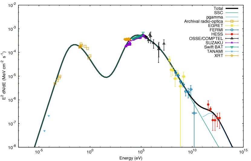
Figure 1.— SED of the Cen A core with our model fit (black line). The green line is a SSC fit to the TANAMI VLBI (Ojha et al., 2010), archival (Marconi et al., 2000), Suzaku (Markowitz et al., 2007), Swift-XRT (Kalberla et al., 2005), Swift-BAT (Ajello et al., 2009), COMPTEL (Steinle et al., 1998), EGRET (Hartman et al., 1999; Sreekumar et al., 1999) and Fermi-LAT (Abdo & et al., 2010) data. The blue line is a fit to the HESS (Aharonian & et al., 2009) data using the $\pi^{0}$ decay product from p$\gamma$ interactions.

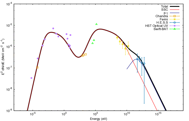
Figure 2.— SED of the M87 core with our model fit (black line). The red line is a SSC fit to the VLA - HST (Biretta et al., 1991; Despringre et al., 1996; Sparks et al., 1996; Kovalev et al., 2007; Perlman et al., 2001; Shi et al., 2007; Tan et al., 2008), Swift-BAT (Ajello et al., 2009), Chandra (Marshall et al., 2002). The blue line is a fit to the HESS (Aharonian et al., 2006) data using the $\pi^{0}$ decay product from p$\gamma$ interactions.

.

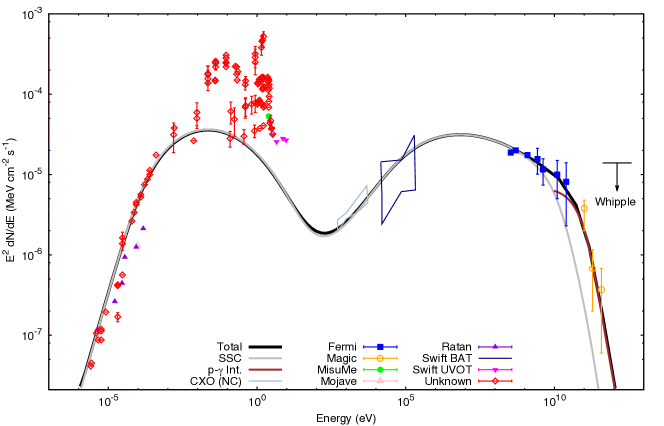
Figure 3.— SED of the NGC1275 core with our model fit (black line). The gray line is a SSC fit to the RATAN (Kovalev et al., 1999), MOVAVE (Lister et al., 2009) , MITSuME (Kotani et al., 2005), Swift-BAT (Ajello et al., 2009), Swift-UVOT (Roming et al., 2005) and Fermi-LAT (Abdo & et al., 2009a) data. The red line is a fit to the Magic (Aleksić & et al., 2010) data using the $\pi^{0}$ decay product from p$\gamma$ interactions. Whipple upper limit is included (Perkins et al., 2006).

.

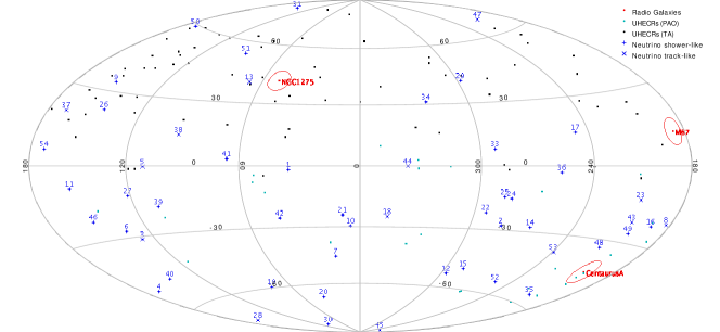
Figure 4.— Skymap in equatorial coordinates of UHECRs, neutrino events and ll AGN. Black and green points are the UHECRs reported by TA and PAO Collaborations, respectively. In blue are the neutrino events (X for like-track and + for like-shower) reported by IceCube Collaboration. For the closest RGs we reported the Cen A, M87 and NGC 1275 positions with red circles of $5^{\circ}$ around them.

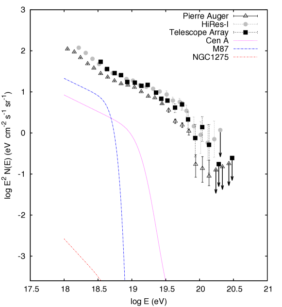
Figure 5.— The UHECR spectra collected with PAO (The Pierre Auger Collaboration et al., 2011), HiRes (High Resolution Fly’S Eye Collaboration et al., 2009) and TA (Abu-Zayyad et al., 2013) experiment are overlapped with UHE proton fluxes of RGs (Cen A, M87 and NGC1275) resulting from extrapolating the proton fluxes used to describe the TeV $\gamma$-ray spectra.

.

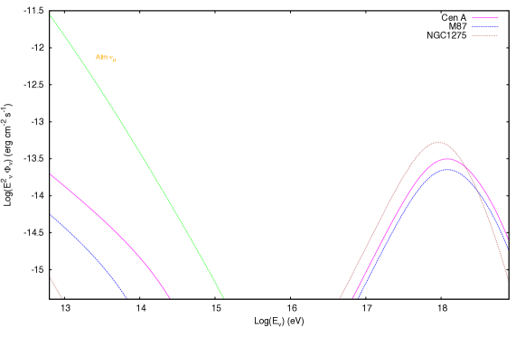
Figure 6.— Neutrino spectra of RGs (Cen A, M87 and NGC1275) obtained as $\pi^{\pm}$ decay products from p$\gamma$ interactions of Fermi-accelerated protons with the seed photons around the first and second SED peaks. The atmospheric muon neutrino background is also shown.

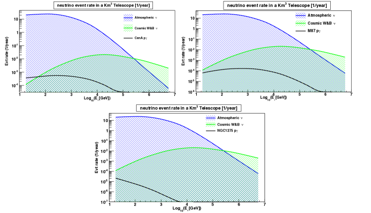
Figure 7.— Neutrino signal to noise ratio for a Km³ neutrino telescope for Cen A (left), M87 (right) and NGC1275 (below). The black lines represent the neutrino signal produced by p$\gamma$ interactions respectively. The blue and the green areas represent the atmospheric and diffuse neutrino “background” within a region of 1^∘ around the source position.

Appendix A Tools for fit

The values reported in Table 1 (break energies, spectral index and normalizations) for synchrotron, Compton scattering and p$\gamma$ spectra were obtained as follows.

Synchrotron spectrum

. We require the synchrotron spectrum (eq. 11) with $A_{syn,\gamma}=[0]$, $\alpha_{e}=[1]$, $\epsilon^{syn}_{\gamma,m}=[2]$ and $\epsilon^{syn}_{\gamma,c}=[3]$. Then, it is written as

$$\left[\epsilon^{2}_{\gamma}N(\epsilon_{\gamma})\right]_{\gamma,syn}=[0]\cases{\left(\frac{\epsilon_{\gamma}}{[2]}\right)^{\frac{4}{3}}&$\epsilon_{\gamma}<[2]$,\cr\left(\frac{\epsilon_{\gamma}}{[2]}\right)^{-\frac{[1]-3}{2}}&$[2]<\epsilon_{\gamma}<[3]$,\cr\left(\frac{[3]}{[2]}\right)^{-\frac{[1]-3}{2}}\left(\frac{\epsilon_{\gamma}}{[3]}\right)^{-\frac{[1]-2}{2}},&$[3]<\epsilon_{\gamma}$\,.\cr}$$ (A1)

Compton scattering spectrum

. Given the Compton scattering spectrum (eq. 18) and doing $A_{ssc,\gamma}=[4]$, $\epsilon^{ssc}_{\gamma,m}=[5]$ and $\epsilon^{ssc}_{\gamma,c}=[6]$, this spectrum is in the form

$$\left[\epsilon^{2}_{\gamma}N(\epsilon_{\gamma})\right]_{\gamma,ssc}=[4]\cases{\left(\frac{\epsilon_{\gamma}}{[5]}\right)^{\frac{4}{3}}&$\epsilon_{\gamma}<[5]$,\cr\left(\frac{\epsilon_{\gamma}}{[5]}\right)^{-\frac{[1]-3}{2}}&$[5]<\epsilon_{\gamma}<[6]$,\cr\left(\frac{[6]}{[5]}\right)^{-\frac{[1]-3}{2}}\left(\frac{\epsilon_{\gamma}}{[6]}\right)^{-\frac{[1]-2}{2}},&$[6]<\epsilon_{\gamma}$\,.\cr}$$ (A2)

P$\gamma$ spectrum

. Considering p$\gamma$ spectrum (eq. 33) with $A_{p\gamma}=[7]$ and $\alpha_{p}=[8]$, then it can be written as

$$\left[\epsilon^{2}_{\gamma}N(\epsilon_{\gamma})\right]_{\gamma,\pi^{0}}=[7]\cases{\left(\frac{\epsilon^{\pi^{0}}_{\gamma,c}}{\epsilon_{0}}\right)^{-1}\left(\frac{\epsilon_{\gamma}}{\epsilon_{0}}\right)^{-[8]+3}&$\epsilon_{\gamma}<\epsilon^{\pi^{0}}_{\gamma,c}$\cr\left(\frac{\epsilon_{\gamma}}{\epsilon_{0}}\right)^{-[8]+2}&$\epsilon^{\pi^{0}}_{\gamma,c}<\epsilon_{\gamma}$\,.\cr}$$ (A3)

We use the method of Chi-square $\chi^{2}$ minimization as implemented in the ROOT software package (Brun & Rademakers, 1997).

References

- Aartsen et al. (2013) Aartsen, M. G., Abbasi, R., Abdou, Y., et al. 2013, Physical Review Letters, 111, 021103
- Aartsen et al. (2014) Aartsen, M. G., Ackermann, M., Adams, J., et al. 2014, Physical Review Letters, 113, 101101
- Abbasi et al. (2011) Abbasi, R., Abdou, Y., Abu-Zayyad, T., et al. 2011, Phys. Rev. D, 83, 092003
- Abbasi & The Telescope Array Collaboration (2014) Abbasi, R. U., & The Telescope Array Collaboration. 2014, ArXiv e-prints, arXiv:1404.5890
- Abbasi et al. (2005) Abbasi, R. U., Abu-Zayyad, T., Archbold, G., et al. 2005, ApJ, 622, 910
- Abdo & et al. (2009a) Abdo, A. A., & et al. 2009a, ApJ, 699, 31
- Abdo & et al. (2009b) —. 2009b, ApJ, 707, 55
- Abdo & et al. (2010) —. 2010, ApJ, 719, 1433
- Abraham et al. (2010) Abraham, J., Abreu, P., Aglietta, M., et al. 2010, Physical Review Letters, 104, 091101
- Abramowski et al. (2012) Abramowski, A., Acero, F., Aharonian, F., et al. 2012, ApJ, 746, 151
- Abreu et al. (2011) Abreu, P., Aglietta, M., Ahn, E. J., et al. 2011, Phys. Rev. D, 84, 122005
- Abu-Zayyad & et al. (2012) Abu-Zayyad, T., & et al. 2012, Nuclear Instruments and Methods in Physics Research A, 689, 87
- Abu-Zayyad et al. (2013) Abu-Zayyad, T., Aida, R., Allen, M., et al. 2013, ApJ, 768, L1
- Acciari & et al. (2009) Acciari, V. A., & et al. 2009, ApJ, 706, L275
- Aharonian & et al. (2005) Aharonian, F., & et al. 2005, A&A, 441, 465
- Aharonian & et al. (2009) —. 2009, ApJ, 695, L40
- Aharonian et al. (2006) Aharonian, F., Akhperjanian, A. G., Bazer-Bachi, A. R., et al. 2006, Science, 314, 1424
- Ahlers & Murase (2014) Ahlers, M., & Murase, K. 2014, Phys. Rev. D, 90, 023010
- Ajello et al. (2009) Ajello, M., Rebusco, P., Cappelluti, N., et al. 2009, ApJ, 690, 367
- Aleksić & et al. (2010) Aleksić, J., & et al. 2010, ApJ, 710, 634
- Aleksić & et al. (2012) —. 2012, A&A, 539, L2
- Aliu et al. (2012) Aliu, E., Arlen, T., Aune, T., et al. 2012, ApJ, 746, 141
- Asada et al. (2006) Asada, K., Kameno, S., Shen, Z.-Q., et al. 2006, PASJ, 58, 261
- Atoyan & Dermer (2001) Atoyan, A., & Dermer, C. D. 2001, Physical Review Letters, 87, 221102
- Bahcall & Waxman (2001) Bahcall, J., & Waxman, E. 2001, Phys. Rev. D, 64, 023002
- Baity & et al. (1981) Baity, W. A., & et al. 1981, ApJ, 244, 429
- Barr et al. (2004) Barr, G. D., Gaisser, T. K., Lipari, P., Robbins, S., & Stanev, T. 2004, Phys. Rev. D, 70, 023006
- Barr et al. (2006) Barr, G. D., Robbins, S., Gaisser, T. K., & Stanev, T. 2006, Phys. Rev. D, 74, 094009
- Becker (2008) Becker, J. K. 2008, Phys. Rep., 458, 173
- Bicknell & Begelman (1996) Bicknell, G. V., & Begelman, M. C. 1996, ApJ, 467, 597
- Biretta et al. (1991) Biretta, J. A., Stern, C. P., & Harris, D. E. 1991, AJ, 101, 1632
- Bowyer et al. (1970) Bowyer, C. S., Lampton, M., Mack, J., & de Mendonca, F. 1970, ApJ, 161, L1
- Brown & Adams (2011) Brown, A. M., & Adams, J. 2011, MNRAS, 413, 2785
- Brun & Rademakers (1997) Brun, R., & Rademakers, F. 1997, Nuclear Instruments and Methods in Physics Research A, 389, 81
- Cuoco & Hannestad (2008) Cuoco, A., & Hannestad, S. 2008, Phys. Rev. D, 78, 023007
- Dermer et al. (2014) Dermer, C. D., Murase, K., & Inoue, Y. 2014, Journal of High Energy Astrophysics, 3, 29
- Dermer et al. (2009) Dermer, C. D., Razzaque, S., Finke, J. D., & Atoyan, A. 2009, New Journal of Physics, 11, 065016
- Despringre et al. (1996) Despringre, V., Fraix-Burnet, D., & Davoust, E. 1996, A&A, 309, 375
- Engel (2008) Engel, R. 2008, in International Cosmic Ray Conference, Vol. 4, International Cosmic Ray Conference, 385–388
- Ferrarese et al. (2007) Ferrarese, L., Mould, J. R., Stetson, P. B., et al. 2007, ApJ, 654, 186
- Fraija (2014a) Fraija, N. 2014a, ApJ, 783, 44
- Fraija (2014b) —. 2014b, MNRAS, 441, 1209
- Fraija (2014c) —. 2014c, MNRAS, 437, 2187
- Fraija (2015) —. 2015, Astroparticle Physics, 71, 1
- Fraija (2016) —. 2016, Journal of High Energy Astrophysics, 9, 25
- Fraija et al. (2012) Fraija, N., González, M. M., Perez, M., & Marinelli, A. 2012, ApJ, 753, 40
- Fraija & Marinelli (2015) Fraija, N., & Marinelli, A. 2015, Astroparticle Physics, 70, 54
- Fraija et al. (2015) Fraija, N., Marinelli, A., Luviano-Valenzuela, U., Galván-Gaméz, A., & Peterson-Bórquez, C. 2015, in IAU Symposium, Vol. 313, Extragalactic Jets from Every Angle, ed. F. Massaro, C. C. Cheung, E. Lopez, & A. Siemiginowska, 175–176
- Franceschini et al. (2008) Franceschini, A., Rodighiero, G., & Vaccari, M. 2008, A&A, 487, 837
- Gaggero et al. (2015) Gaggero, D., Grasso, D., Marinelli, A., Urbano, A., & Valli, M. 2015, ApJ, 815, L25
- Georganopoulos et al. (2005) Georganopoulos, M., Perlman, E. S., & Kazanas, D. 2005, ApJ, 634, L33
- Gorham et al. (2010) Gorham, P. W., Allison, P., Baughman, B. M., et al. 2010, Phys. Rev. D, 82, 022004
- Gorham et al. (2012) —. 2012, Phys. Rev. D, 85, 049901
- Halzen (2007) Halzen, F. 2007, Ap&SS, 309, 407
- Hardcastle (2010) Hardcastle, M. J. 2010, MNRAS, 405, 2810
- Hardcastle et al. (2009) Hardcastle, M. J., Cheung, C. C., Feain, I. J., & Stawarz, Ł. 2009, MNRAS, 393, 1041
- Hardcastle et al. (2003) Hardcastle, M. J., Worrall, D. M., Kraft, R. P., et al. 2003, ApJ, 593, 169
- Hardcastle et al. (2007) Hardcastle, M. J., Kraft, R. P., Sivakoff, G. R., et al. 2007, ApJ, 670, L81
- Hartman et al. (1999) Hartman, R. C., Bertsch, D. L., Bloom, S. D., et al. 1999, ApJS, 123, 79
- High Resolution Fly’S Eye Collaboration et al. (2009) High Resolution Fly’S Eye Collaboration, Abbasi, R. U., Abu-Zayyad, T., et al. 2009, Astroparticle Physics, 32, 53
- Hillas (1984) Hillas, A. M. 1984, ARA&A, 22, 425
- Horiuchi et al. (2006) Horiuchi, S., Meier, D. L., Preston, R. A., & Tingay, S. J. 2006, PASJ, 58, 211
- IceCube Collaboration (2013) IceCube Collaboration. 2013, Science, 342, arXiv:1311.5238
- Jiang et al. (2010) Jiang, Y.-Y., Hou, L. G., Han, J. L., Sun, X. H., & Wang, W. 2010, ApJ, 719, 459
- Junor et al. (1999) Junor, W., Biretta, J. A., & Livio, M. 1999, Nature, 401, 891
- Kadler et al. (2016) Kadler, M., Krauß, F., Mannheim, K., et al. 2016, ArXiv e-prints, arXiv:1602.02012
- Kalashev et al. (2014) Kalashev, O., Semikoz, D., & Tkachev, I. 2014, ArXiv e-prints, arXiv:1410.8124
- Kalberla et al. (2005) Kalberla, P. M. W., Burton, W. B., Hartmann, D., et al. 2005, A&A, 440, 775
- Kellermann et al. (2004) Kellermann, K. I., Lister, M. L., Homan, D. C., et al. 2004, ApJ, 609, 539
- Khiali & de Gouveia Dal Pino (2016) Khiali, B., & de Gouveia Dal Pino, E. M. 2016, MNRAS, 455, 838
- Khiali et al. (2015) Khiali, B., de Gouveia Dal Pino, E. M., & Sol, H. 2015, ArXiv e-prints, arXiv:1504.07592
- Kimura et al. (2015) Kimura, S. S., Murase, K., & Toma, K. 2015, ApJ, 806, 159
- Kotani et al. (2005) Kotani, T., Kawai, N., Yanagisawa, K., et al. 2005, Nuovo Cimento C Geophysics Space Physics C, 28, 755
- Kovalev et al. (2007) Kovalev, Y. Y., Lister, M. L., Homan, D. C., & Kellermann, K. I. 2007, ApJ, 668, L27
- Kovalev et al. (1999) Kovalev, Y. Y., Nizhelsky, N. A., Kovalev, Y. A., et al. 1999, A&AS, 139, 545
- Kravchenko et al. (2012) Kravchenko, I., Hussain, S., Seckel, D., et al. 2012, Phys. Rev. D, 85, 062004
- Lemoine & Waxman (2009) Lemoine, M., & Waxman, E. 2009, J. Cosmology Astropart. Phys., 11, 9
- Lenain et al. (2008) Lenain, J.-P., Boisson, C., Sol, H., & Katarzyński, K. 2008, A&A, 478, 111
- Lister et al. (2009) Lister, M. L., Aller, H. D., Aller, M. F., et al. 2009, AJ, 137, 3718
- Liu & Wang (2013) Liu, R.-Y., & Wang, X.-Y. 2013, ApJ, 766, 73
- Longair (1994) Longair, M. S. 1994, High energy astrophysics. Volume 2. Stars, the Galaxy and the interstellar medium.
- Ly et al. (2007) Ly, C., Walker, R. C., & Junor, W. 2007, ApJ, 660, 200
- Marconi et al. (2000) Marconi, A., Schreier, E. J., Koekemoer, A., et al. 2000, ApJ, 528, 276
- Marinelli et al. (2014) Marinelli, A., Fraija, N., & Patricelli, B. 2014, ArXiv e-prints, arXiv:1410.8549
- Markowitz et al. (2007) Markowitz, A., Takahashi, T., Watanabe, S., et al. 2007, ApJ, 665, 209
- Marshall et al. (2002) Marshall, H. L., Miller, B. P., Davis, D. S., et al. 2002, ApJ, 564, 683
- Mücke & Protheroe (2001) Mücke, A., & Protheroe, R. J. 2001, Astroparticle Physics, 15, 121
- Murase & Beacom (2010) Murase, K., & Beacom, J. F. 2010, Phys. Rev. D, 81, 123001
- Murase et al. (2012) Murase, K., Dermer, C. D., Takami, H., & Migliori, G. 2012, ApJ, 749, 63
- Murase et al. (2014) Murase, K., Inoue, Y., & Dermer, C. D. 2014, Phys. Rev. D, 90, 023007
- Murase & Ioka (2013) Murase, K., & Ioka, K. 2013, Physical Review Letters, 111, 121102
- Mushotzky et al. (1976) Mushotzky, R. F., Baity, W. A., Wheaton, W. A., & Peterson, L. E. 1976, ApJ, 206, L45
- Nagai et al. (2014) Nagai, H., Haga, T., Giovannini, G., et al. 2014, ApJ, 785, 53
- Ojha et al. (2010) Ojha, R., Kadler, M., Böck, M., et al. 2010, ArXiv e-prints, arXiv:1001.0059
- Padovani et al. (2015) Padovani, P., Petropoulou, M., Giommi, P., & Resconi, E. 2015, MNRAS, 452, 1877
- Perkins et al. (2006) Perkins, J. S., Badran, H. M., Blaylock, G., et al. 2006, ApJ, 644, 148
- Perlman et al. (2001) Perlman, E. S., Sparks, W. B., Radomski, J., et al. 2001, ApJ, 561, L51
- Petropoulou et al. (2015) Petropoulou, M., Dimitrakoudis, S., Padovani, P., Mastichiadis, A., & Resconi, E. 2015, MNRAS, 448, 2412
- Petropoulou et al. (2014a) Petropoulou, M., Giannios, D., & Dimitrakoudis, S. 2014a, MNRAS, 445, 570
- Petropoulou et al. (2014b) Petropoulou, M., Lefa, E., Dimitrakoudis, S., & Mastichiadis, A. 2014b, A&A, 562, A12
- Pierre Auger Collaboration & et al. (2007) Pierre Auger Collaboration, & et al. 2007, Science, 318, 938
- Pierre Auger Collaboration & et al. (2008) —. 2008, Astroparticle Physics, 29, 188
- Razzaque (2013) Razzaque, S. 2013, Phys. Rev. D, 88, 103003
- Razzaque et al. (2012) Razzaque, S., Dermer, C. D., & Finke, J. D. 2012, ApJ, 745, 196
- Roming et al. (2005) Roming, P. W. A., Kennedy, T. E., Mason, K. O., et al. 2005, Space Sci. Rev., 120, 95
- Rybicki & Lightman (1986) Rybicki, G. B., & Lightman, A. P. 1986, Radiative Processes in Astrophysics
- Ryu et al. (2010) Ryu, D., Das, S., & Kang, H. 2010, ApJ, 710, 1422
- Sahakyan et al. (2013) Sahakyan, N., Yang, R., Aharonian, F. A., & Rieger, F. M. 2013, ApJ, 770, L6
- Sahu et al. (2012) Sahu, S., Zhang, B., & Fraija, N. 2012, Phys. Rev. D, 85, 043012
- Sari & Esin (2001) Sari, R., & Esin, A. A. 2001, ApJ, 548, 787
- Schoenen & Raedel (2015) Schoenen, S., & Raedel, L. 2015, The Astronomer’s Telegram, 7856, 1
- Shi et al. (2007) Shi, Y., Rieke, G. H., Hines, D. C., Gordon, K. D., & Egami, E. 2007, ApJ, 655, 781
- Sommers (2001) Sommers, P. 2001, Astroparticle Physics, 14, 271
- Sparks et al. (1996) Sparks, W. B., Biretta, J. A., & Macchetto, F. 1996, ApJ, 473, 254
- Sreekumar et al. (1999) Sreekumar, P., Bertsch, D. L., Hartman, R. C., Nolan, P. L., & Thompson, D. J. 1999, Astroparticle Physics, 11, 221
- Stanev (1997) Stanev, T. 1997, ApJ, 479, 290
- Stecker (1968) Stecker, F. W. 1968, Physical Review Letters, 21, 1016
- Stecker (2013) —. 2013, Phys. Rev. D, 88, 047301
- Steinle et al. (1998) Steinle, H., Bennett, K., Bloemen, H., et al. 1998, A&A, 330, 97
- Strauss et al. (1992) Strauss, M. A., Huchra, J. P., Davis, M., et al. 1992, ApJS, 83, 29
- Tamborra & Ando (2015) Tamborra, I., & Ando, S. 2015, J. Cosmology Astropart. Phys., 9, 36
- Tan et al. (2008) Tan, J. C., Beuther, H., Walter, F., & Blackman, E. G. 2008, ApJ, 689, 775
- Tavecchio & Ghisellini (2015) Tavecchio, F., & Ghisellini, G. 2015, MNRAS, 451, 1502
- Tavecchio et al. (1998) Tavecchio, F., Maraschi, L., & Ghisellini, G. 1998, ApJ, 509, 608
- Taylor et al. (2006) Taylor, G. B., Gugliucci, N. E., Fabian, A. C., et al. 2006, MNRAS, 368, 1500
- The Pierre Auger Collaboration et al. (2011) The Pierre Auger Collaboration, Abreu, P., Aglietta, M., et al. 2011, ArXiv e-prints, arXiv:1107.4809
- Tonry (1991) Tonry, J. L. 1991, ApJ, 373, L1
- Unger et al. (2007) Unger, M., Engel, R., Schüssler, F., Ulrich, R., & Pierre Auger Collaboration. 2007, Astronomische Nachrichten, 328, 614
- Vermeulen et al. (1994) Vermeulen, R. C., Readhead, A. C. S., & Backer, D. C. 1994, ApJ, 430, L41
- Walker et al. (2000) Walker, R. C., Dhawan, V., Romney, J. D., Kellermann, K. I., & Vermeulen, R. C. 2000, ApJ, 530, 233
- Waxman (1998) Waxman, E. 1998, in 19th Texas Symposium on Relativistic Astrophysics and Cosmology, ed. J. Paul, T. Montmerle, & E. Aubourg
- Waxman & Bahcall (1997) Waxman, E., & Bahcall, J. 1997, Phys. Rev. Lett., 78, 2292
- Waxman & Bahcall (1999) Waxman, E., & Bahcall, J. 1999, Phys. Rev. D, 59, 023002
- Winkler & White (1975) Winkler, Jr., P. F., & White, A. E. 1975, ApJ, 199, L139
- Yamamoto (2008) Yamamoto, T. 2008, in International Cosmic Ray Conference, Vol. 4, International Cosmic Ray Conference, 335–338
.
.
.