Impulse-induced generation of stationary and moving discrete breathers in nonlinear oscillator networks

Abstract

We study discrete breathers in prototypical nonlinear oscillator networks subjected to non-harmonic zero-mean periodic excitations. We show how the generation of stationary and moving discrete breathers are optimally controlled by solely varying the impulse transmitted by the periodic excitations, while keeping constant the excitation’s amplitude and period. Our theoretical and numerical results show that the enhancer effect of increasing values of the excitation’s impulse, in the sense of facilitating the generation of stationary and moving breathers, is due to a correlative increase of the breather’s action and energy.

I Introduction

Discrete breathers are intrinsic localized modes that can emerge in networks of coupled nonlinear oscillators breather_reviews ; Aubry . They have been observed not only in Hamiltonian lattices but also in driven dissipative systems under certain conditions. Discrete breathers have been theoretically predicted or experimentally generated in a wide variety of physical systems such as Josephson junction arrays JJ , coupled pendula chains pendula , micro- and macro-mechanical cantilever arrays cantilever , granular crystals granular , nonlinear electrical lattices electric , and double-strand DNA models DNA , just to cite a few instances.

Up to now, breathers have been mainly studied for the case of a harmonic external excitation, while various types of periodic excitations are in principle possible, depending upon the physical context under consideration. Since there are infinitely many different wave forms, a quite natural question is to ask how the generation and dynamics of breathers are affected by the presence of a generic periodic excitation.

In this present work, we show that a relevant quantity properly characterizing the effectiveness of zero-mean periodic excitations $F(t)$ having equidistant zeros at controlling the generation and dynamics of discrete breathers is the impulse transmitted by the external excitation over a half-period (hereafter referred to simply as the excitation’s impulse 1 , $I\equiv\int_{0}^{T/2}F(t)dt$, $T$ being the period)$-$ a quantity integrating the conjoint effects of the excitation’s amplitude, period, and waveform. It is worth mentioning that the relevance of the excitation’s impulse has been observed previously in quite different contexts, such as ratchet transport 2 , adiabatically ac driven periodic (Hamiltonian) systems 3 , driven two-level systems and periodically curved waveguide arrays 4 , chaotic dynamics of a pump-modulation Nd:YVO₄ laser 5 , topological amplification effects in scale-free networks of signaling devices 6 , and controlling chaos in starlike networks of dissipative nonlinear oscillators 7 .

The rest of this paper is organized as follows. In Sec. II we introduce the model and further comment on some of its main features. Section III provides numerical evidence for the essential role of the excitation’s impulse at generating breathers and controlling their stability for the prototypical cases of a hard $\phi^{4}$ potential and a sine-Gordon potential. A theoretical explanation of the effectiveness of the excitation’s impulse in terms of energy and action is provided in Sec. IV. Finally, Sec. V is devoted to a discussion of the major findings and of some open problems.

II Model system

The discrete nonlinear Klein–Gordon equation with linear coupling, linear damping, and external periodic excitation is one of the simplest equations where dissipative discrete breathers may arise:

$$\ddot{u}_{n}+\alpha\dot{u}_{n}+V^{\prime}(u_{n})+C(2u_{n}-u_{n+1}-u_{n-1})=F(t),$$ (1)

in which $V(u_{n})$ is an on–site (substrate) potential, $\alpha$ is the damping constant, $C$ is the coupling constant, while $F(t)$ is a zero-mean periodic excitation.

$$F(t)=(-1)^{hn}f_{0}f_{1,2}(t),$$ (2)

in which $f_{0}$ is the driving amplitude, $h$ is a hardness parameter whose value is $0$ ($1$) when the on-site potential is soft (hard), while $f_{1}(t)$, $f_{2}(t)$ are two different periodic excitations that we will use as illustrative examples to show that the impulse is the relevant quantity controlling the effect of the external excitation on the generation and stability properties of breathers. These periodic excitations are given by

$$f_{1}(t)=N(m)\mathrm{sn}\left(\frac{2K(m)\omega_{\mathrm{b}}t}{\pi};m\right)\mathrm{dn}\left(\frac{2K(m)\omega_{\mathrm{b}}t}{\pi};m\right),$$ (3)

$$f_{2}(t)=\mathrm{sn}\left(\frac{2K(m)\omega_{\mathrm{b}}t}{\pi};m\right),$$ (4)

where $\mathrm{sn}(\cdot)\equiv\mathrm{sn}(\cdot;m)$ and $\mathrm{dn}(\cdot)\equiv\mathrm{dn}(\cdot;m)$ are Jacobian elliptic functions of parameter $m$ [$K\equiv K(m)$ is the complete elliptic integral of the first kind], while $N(m)$ is a normalization function which is introduced for the elliptic excitation $f_{1}(t)$ to have the same amplitude $f_{0}$ and period $T\equiv 2\pi/\omega_{\mathrm{b}}$ for any wave form (i.e., $\forall m\in\left[0,1\right)$ ). Specifically, the normalization function is given by

$$N(m)=\left[\eta_{1}+\frac{\eta_{2}}{1-\exp[(m-\eta_{3})/\eta_{4}]}\right]^{-1},$$ (5)

with $\eta_{1}=0.43932$, $\eta_{2}=0.69796$, $\eta_{3}=0.37270$, $\eta_{4}=0.26883$. In both excitations $f_{1,2}(t)$, when $m=0$, then $F(t)=(-1)^{hn}f_{0}\sin\left(\omega_{\mathrm{b}}t\right)$, that is, one recovers the standard case of a harmonic excitation Cubero , whereas, for the limiting value $m=1$, the excitation $f_{1}(t)$ vanishes while the excitation $f_{2}(t)$ reduces to a square wave. It is worth noting that the excitations $f_{1,2}(t)$ have been chosen to exhibit the following properties. For the excitation $f_{1}(t)$, its impulse per unit of amplitude, $I_{1}(m)/I_{1}(0)$ with $I_{1}(m)=TN(m)/\left[2K(m)\right]$, presents a single maximum at $m=m_{\max}\simeq 0.717$. For the excitation $f_{2}(t)$, its impulse is written $I_{2}(m)=T\mathrm{arctanh}(\sqrt{m})/\left[2\sqrt{m}K(m)\right]$, and hence it corresponding normalized impulse $I_{2}(m)/I_{2}(0)$ grows monotonically from $1$ to $1.5$. Figure 1 shows the time-dependence of both excitations over a period together with the dependence of their respective normalized impulses on the shape parameter $m$.

The use of Jabobian elliptic functions as periodic excitations is mainly motivated by the fact that, after normalizing their (natural) arguments to keep the period as a fixed independent parameter, their waveforms can be changed by solely varying a single parameter: the elliptic parameter $m$, and hence the corresponding impulse will only depend on $m$ once the amplitude and period are fixed.

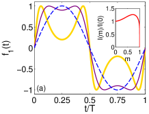
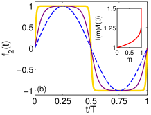
Figure 1: External excitations (3) and (4) vs time over a period (panels (a) and (b), respectively). In the former case, dashed (blue), thin (purple), and thick (golden) lines correspond to $m=0$, $m=m_{\max}=0.717$, and $m=0.99$, respectively. In the latter case, the same lines correspond to $m=0$, $m=0.99,$ and $m=1-10^{-14}$, respectively. Notice that, when $m\rightarrow 1$, the excitation $f_{2}$ becomes a square wave signal while $f_{1}$ vanishes. The insets show the respective normalized impulses of the excitations vs the shape parameter (see the text).

The aim of this paper is to study the effectiveness of the excitation’s impulse at controlling breathers arising in Eq. (1) by considering two prototypical on–site potentials. First, a hard $\phi^{4}$ potential, which was previously considered in Cubero for the limiting case of a harmonic excitation $\left(m=0\right)$, and where it was shown that there exists a threshold value of $f_{0}$ such that breathers do not exist below it. Remarkably, such a threshold amplitude can be decreased in the presence of noise through a stochastic resonance mechanism. Second, a sine-Gordon potential Marin so that Eq. (1) becomes the so-called Frenkel–Kontorova model (see, e.g., Refs. Kivshar ; sG for additional details), in which the emergence of discrete moving breathers moving is indicated by the existence of a pitchfork bifurcation together with the appearance of an intermediate state.

The existence of discrete breathers is characterized by using techniques based on the anti-continuous (AC) limit AClimit . Thus, two periodic attractors must be found in such a limit (i.e., for the corresponding isolated nonlinear oscillator) such that the attractor with the largest amplitude is assigned to the central ($n=0$) site of the chain, while the other periodic attractor is assigned to the rest of the coupled oscillators. Such a solution is then continued from $C=0$ to the prescribed value of $C$. Since discrete breathers are periodic orbits in phase space, they can be calculated by means of a shooting method, i.e., they can be considered as fixed points of the map:

$$\left[\{u_{n}(0)\},\{\dot{u}_{n}(0)\}\right]\rightarrow\left[\{u_{n}(T)\},\{\dot{u}_{n}(T)\}\right].$$ (6)

This analysis is accomplished by using a Powell hybrid algorithm complemented by an 5th-6th order Runge–Kutta–Verner integrator. To study the stability of discrete breathers, a small perturbation $\xi_{n}$ is introduced to a given $u_{n0}$ solution of Eq. (1) according to $u_{n}=u_{n0}+\xi_{n}$. Thus, one obtains the equation which is verified (to first order) by $\xi_{n}$:

$$\ddot{\xi}_{n}+\alpha\dot{\xi}_{n}+V^{\prime\prime}(u_{n0})\xi_{n}+C(2\xi_{n}-\xi_{n+1}-\xi_{n-1})=0.$$ (7)

To determine the orbital stability of periodic orbits, a Floquet analysis can be performed so that the stability properties are deduced from the spectrum of the Floquet operator (whose matrix representation is the monodromy $\mathcal{M}$), given by

$$\left[\{\xi_{n}(T)\},\{\dot{\xi}_{n}(0)\}\right]^{T}=\mathcal{M}\left[\{\xi_{n}(0)\},\{\dot{\xi}_{n}(0)\}\right]^{T},$$ (8)

where $\lambda=\exp(i\theta)$ are the Floquet multipliers while the values of $\theta$ are the Floquet exponents. All eigenvalues must lie inside the unit circle if the breather is stable.

III Numerical results

Our numerical study starts with the case of a hard $\phi^{4}$ potential, that is, $V(u)=u^{2}/2+u^{4}/4$. Notice that breathers in such a potential exhibit staggered tails due to its hardness. This means that the system must be driven following this pattern by taking $h=1$ in (2) (see Figs. 2(a) and 2(b)). It has been shown for $m=0$ Cubero that breathers exist if $f_{0}>f_{\mathrm{th}}$, i.e., the excitation amplitude must surpass a certain threshold. In general, this threshold is a function of the system parameters. Here we study the dependence of this threshold on the shape parameter $m$, while keeping fixed the remaining parameters. Figure 2(c) shows this dependence for the parameters $\alpha=0.1$, $C=1$, $\omega_{\mathrm{b}}=5$.

For the excitation $f_{1}(t)$ (3), it should be emphasized the existence of a minimum threshold at a critical value $m=m_{c}\approx 0.664$ for such set of parameters; however, if any of such parameters were varied, $m_{c}$ would remain close to such a value. Although this critical value does not exactly match the value $m=$ $m_{\max}\approx 0.717$ at which the impulse $I_{1}\left(m\right)$ presents a single maximum, it is very close to the value $m=m_{1}=0.6416$ where the first harmonic of the Fourier expansion of the external driving presents a single maximum. Also, the waveforms corresponding to $m_{c}$ and $m_{\max}$ can be hardly distinguishable, as is shown in Fig. 2(d), which means that the values of their respective impulses are almost identical (the relative difference is only $\sim 0.42\%$). The fact that $m_{c}$ does not change significantly when $\omega_{\mathrm{b}}$ and $C$ are varied implies that this property holds in the AC limit. Indeed, for the isolated oscillator we found that for the largest-amplitude attractor there exists a minimum value of its amplitude, $f_{\mathrm{th}}$, at $m=0.668\approx m_{c}$, while the smallest-amplitude attractor exists for any value of $f_{0}$ (i.e., $f_{\mathrm{th}}=0,\ \forall m$). Thus, the breather seems to inherit this key feature (impulse-induced threshold behaviour) of the largest-amplitude attractor of the isolated oscillator. It is worth mentioning that $\alpha$ must be sufficiently small in order that two periodic attractors can exist in the AC limit.

For the excitation $f_{2}(t)$ (4), we found that the threshold amplitude $f_{\mathrm{th}}$ exhibits a monotonously decreasing behavior as a function of the shape parameter (see 2(c)), as expected from the monotonously increasing behavior of its impulse $I_{2}\left(m\right)$. Thus, the analysis of both periodic excitations $f_{1,2}(t)$ confirmed the same effect of the excitation’s impulse on the amplitude threshold for the existence of breathers.

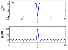
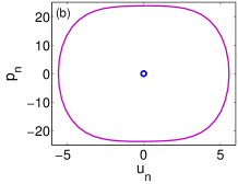
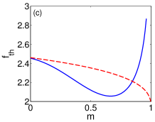
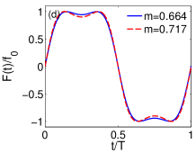
Figure 2: Profiles of $u_{n},p_{n}\equiv\dot{u}_{n}$ (a) and phase space diagrams (b) of a breather in a $\phi^{4}$ chain for $m=0.6$ and $f_{0}=3$. (c) Threshold amplitude for the existence of breathers vs shape parameter $m$. Solid (blue) and dashed (red) lines correspond to excitations (3) and (4), respectively. Notice that in the former case, there exists a minimum at $m=m_{c}=0.664$ for $f_{\mathrm{th}}=2.056$, whereas in the latter case, one sees a monotonously decreasing behavior. (d) External excitation (3) vs time over a period for two values of the shape parameter: $m=m_{c}$, for which $f_{\mathrm{th}}$ is minimum, and $m=m_{\max}=0.717$, for which the impulse is maximum. Fixed parameters: $\alpha=0.1$, $C=1$, $\omega_{\mathrm{b}}=5$.

Next, we consider the Frenkel–Kontorova model, i.e., the case of a sine-Gordon potential: $V^{\prime}(u)=\sin(2\pi u)/(2\pi)$. This case, which was previously analyzed in detail for the limiting case of a harmonic excitation $\left(m=0\right)$ in Marin , is much richer than the previous one due to the existence of exchange of stability bifurcations, Hopf / Neimark-Sacker bifurcations, chaos, moving breathers Meister , and rotobreathers roto . Figure 3 shows the position, velocity, and phase space diagram of a typical breather. Since the sine-Gordon potential is soft, tails are unstaggered and hence one takes $h=0$ in (2) in order that the periodic excitation fit this pattern. According to Ref. Marin , for $\alpha=0.02$ and $f_{0}\gtrsim 0.05$ the largest-amplitude attractor in the AC limit corresponds to a rotation, and hence it cannot be used for the analysis of breathers (the analysis of rotobreathers is beyond the scope of the present work). Thus, we are fixing $\alpha=f_{0}=0.02$ in our numerical simulations. Similarly to the case of a hard $\phi^{4}$ potential, we found a threshold for the existence of breathers inheriting the features of the largest-amplitude attractor of the AC limit . Additionally, we found an interesting behaviour arising from stability exchange bifurcations that leads to the onset of moving breathers moving . In this kind of bifurcations, a site-centered breather (i.e., a breather with a single site excited at the AC limit) undergoes a supercritical pitchfork bifurcation becoming unstable past a critical value of the coupling, $C=C_{1},$ while a new kind of breather appears — the so-called intermediate breather — where two adjacent sites are excited with different amplitudes. This intermediate breather disappears after undergoing a subcritical pitchfork bifurcation at $C=C_{1}^{\prime}$. At this coupling value, a site-centered breather (i.e., a breather with two adjacent sites excited with the same amplitude), which is unstable for $C<C_{1}^{\prime}$, changes its stability (see Fig. 22 in Aubry , and Figs. 5 and 8 in Marin ). Figures 3(c) and 3(d) show the onset of this instability and the dynamics of a moving breather, respectively, for the excitation $f_{1}(t)$. The spatiotemporal patterns of moving breathers is illustrated by plotting their energy density:

$$E_{n}=\frac{\dot{u}_{n}^{2}}{2}+V(u_{n})+\frac{C}{4}\left[(u_{n}-u_{n+1})^{2}+(u_{n}-u_{n-1})^{2}\right].$$ (9)

We found these results for frequencies over the range $1/2<\omega_{\mathrm{b}}<2/3$. Note, however, that over the range $2/3<\omega_{\mathrm{b}}<1$ the discussed phenomenology can change due to the properties of Floquet exponents stab . Indeed, for frequencies over the range $2/3<\omega_{\mathrm{b}}<1$, the breather undergoes a Neimark–Sacker bifurcation as the coupling is increased, making it unstable past a critical coupling value $C=C_{2}$. This instability is characterized by the eventual destruction of the breather (i.e., the localization is lost and only a linear mode remains; see Fig. 4). The critical value $C_{2}$ is much smaller than $C_{1}$ (in fact, $C_{2}$ is close to 0, i.e. to the AC limit). Therefore, it has no sense to study the emergence of moving breathers by stability exchange bifurcations. Note that this does not mean that moving breathers cannot exist for $\omega_{\mathrm{b}}>2/3$. The mechanism for the emergence of breathers when $\omega_{\mathrm{b}}>2/3$ is simply different: it is no more than the spontaneous motion described in Ref. Marin ; Meister . Notice that in Hamiltonian systems, moving breathers exist over this range of frequencies (cf. Kivshar ).

Next, Fig. 5 shows the dependence of the critical values $C_{1},$ $C_{2}$ as functions of the shape parameter $m$. For the excitation $f_{1}(t)$, one sees that $C_{1}$ presents a minimum at $m\approx 0.64$ when $\omega_{\mathrm{b}}=0.2\pi$, while $C_{2}$ presents a minimum at $m\approx 0.67$ when $\omega_{\mathrm{b}}=0.8$. Notice that these values of the shape parameter are significantly close to $0.717\approx m_{\max}$, indicating once more again the effect of the excitation’s impulse. The stability range increases as $m$ is increased from these values (see Fig. 5). However, one expects that the pitchfork and Neimark-Sacker bifurcations disappear as $m\rightarrow 1$ since in such a limit the excitation and the localization vanish. For the excitation $f_{2}(t)$, one sees that $C_{1},C_{2}$ present a monotonously decreasing behavior, as expected from the monotonously increasing behavior of the impulse $I_{2}(m)$. Thus, the analysis of both periodic excitations $f_{1,2}(t)$ confirmed the same effect of the excitation’s impulse on the critical coupling values $C_{1,2}$.

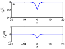
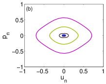
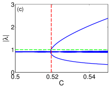
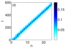
Figure 3: Profiles of $u_{n},p_{n}\equiv\dot{u}_{n}$ (a) and phase space diagrams (b) of a breather in a chain with a sine-Gordon potential for the excitation (3) and $C=0.5$. (c) Modulus of the Floquet multiplier $\lambda$ vs coupling $C$. The dashed vertical line indicates de location of $C_{1}$. (d) Spatiotemporal pattern of the energy density of a moving breather emerging from the unstable solution for $C=0.52$. Fixed parameters: $\alpha=f_{0}=0.02$, $m=0.66$, $\omega_{\mathrm{b}}=0.2\pi$.

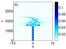
Figure 4: (a) Modulus of the Floquet multiplier $\lambda$ vs coupling $C$ for the excitation (3). The dashed vertical line indicates de location of $C_{2}$. (b) Spatiotemporal pattern of the energy density of an unstable breather for $C=0.1$. This instability finally leads to the destruction of the breather. Fixed parameters: $m=0.66$, $\alpha=f_{0}=0.02$, $\omega_{\mathrm{b}}=0.8$.

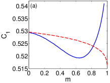
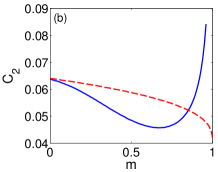
Figure 5: (a) Loci $C_{1}$ (see the text) of the exchange of stability bifurcation (i.e., onset of moving breathers) as a function of the shape parameter $m$ for $\alpha=f_{0}=0.02$, $\omega_{\mathrm{b}}=0.2\pi$. (b) Loci $C_{2}$ (see the text) of Neimark–Sacker bifurcation as a function of the shape parameter $m$ for $\alpha=f_{0}=0.02$, $\omega_{\mathrm{b}}=0.8$. Solid (blue) and dashed (red) lines correspond to excitations (3) and (4), respectively.

IV Discussion

The numerical results discussed in Sec. III may be understood by considering the excitation’s impulse through an energy-based analysis, including the properties of the action, of isolated oscillators. For the sake of clarity, we will consider, for example, the excitation $f_{1}(t)$ (3) in the subsequent analysis. Indeed, every breather possesses a tail due to its localized character while the oscillators forming this tail effectively behave as linear oscillators presenting a small-amplitude attractor. Consequently, a breather can inherit some properties associated with the effective linear character of the oscillators forming its tail. We found indeed that breathers inherit the dependence on the shape parameter according to the impulse principle. Thus, we analyze the response of a linear (harmonic) oscillator subjected to a periodic anti-symmetric driving:

$$\ddot{u}+\alpha\dot{u}+\omega_{0}^{2}u=f_{0}\sum_{k=0}^{\infty}G_{2k+1}\sin\left[(2k+1)\omega_{\mathrm{b}}t\right],$$ (10)

where $G_{2k+1}$ are the Fourier coefficients of the non-harmonic excitation (3):

$$G_{k}=\frac{\pi^{2}N(m)k}{2\sqrt{m}K^{2}(m)}\mathrm{sech}\left[\frac{k\pi K(1-m)}{2K(m)}\right].$$ (11)

After some straightforward algebra, one obtains the solution

$$u(t)=\sum_{k=0}^{\infty}\left[A_{2k+1}\cos\left((2k+1)\omega_{\mathrm{b}}t\right)+B_{2k+1}\sin\left((2k+1)\omega_{\mathrm{b}}t\right)\right],$$ (12)

where

$$A_{k} =f_{0}\frac{\omega_{0}^{2}-k^{2}\omega_{\mathrm{b}}^{2}}{k^{2}\omega^{2}\alpha^{2}+(\omega_{0}^{2}-k^{2}\omega_{\mathrm{b}}^{2})^{2}}G_{k},$$

$$B_{k} =f_{0}\frac{-k\omega_{\mathrm{b}}\alpha}{k^{2}\omega_{\mathrm{b}}^{2}\alpha^{2}+(\omega_{0}^{2}-k^{2}\omega_{\mathrm{b}}^{2})^{2}}G_{k}.$$ (13)

The action $J\equiv\frac{1}{2\pi}\oint\dot{u}\mathrm{d}u$ can be recast into the form

$$J=\frac{1}{\pi}\int_{0}^{T/2}\left(\dot{u}(t)\right)^{2}\mathrm{d}t=\frac{\omega}{2}\sum_{k=0}^{\infty}k^{2}(A_{k}^{2}+B_{k}^{2}),$$ (14)

with $T=2\pi/\omega_{\mathrm{b}}$ being the oscillator’s period. Thus, the action of the linear oscillator can be finally expressed as

$$J =\frac{\omega_{\mathrm{b}}f_{0}}{2}\sum_{k=0}^{\infty}\mu_{2k+1}G_{2k+1}^{2},$$

$$\mu_{k} =k^{2}\frac{(\omega_{0}^{2}-k^{2}\omega_{\mathrm{b}}^{2})^{2}+k^{2}\omega_{\mathrm{b}}^{2}\alpha^{2}}{[k^{2}\omega_{\mathrm{b}}^{2}\alpha^{2}+(\omega_{0}^{2}-k^{2}\omega_{\mathrm{b}}^{2})^{2}]^{2}}.$$ (15)

Notice that $\mu_{k}$ does not depend on the particular waveform of the external periodic excitation $F(t)$, but depends on $\omega_{\mathrm{b}}$ and $\alpha$. Then, the dependence of the action on the shape parameter $m$ appears only in the $G_{k}^{2}$ terms. Now, after taking into account the fast decay of the Fourier coefficients with $k$, one numerically finds that the action presents a single maximum at $m=m_{\ell}$ which is very close to $m_{1}$, where $m_{1}$ is the shape parameter value at which $G_{1}$ presents a single maximum (recall from Sec. III that $m_{1}=0.6416$). Notice that $m_{\ell}$ depends on $\mu_{k}$ and, consequently, on $\omega_{\mathrm{b}}$ and $\alpha$. For instance, for the parameters sets taken in Figs. 2 and 4, i.e. ($\alpha=0.1$, $\omega_{\mathrm{b}}=5$) and ($\alpha=0.02$, $\omega_{\mathrm{b}}=0.8$), the value of $m_{\ell}$ is 0.646 and 0.644, respectively.

Remarkably, the above mentioned properties also holds for the corresponding average energies $<E>$, which for the linear oscillator reads:

$$<E>=\int_{0}^{T}\left(\frac{1}{2}\dot{u}^{2}(t)+\frac{\omega_{0}^{2}}{2}u^{2}(t)\right)$$ (16)

For the excitation (3), it can be recast into the simple form

$$<E> =\frac{\pi f_{0}}{2}\sum_{k=0}^{\infty}\mu^{\prime}_{2k+1}G_{2k+1}^{2},$$

$$\mu^{\prime}_{k} =\frac{(k^{2}\omega_{\mathrm{b}}^{2}+\omega_{0}^{2})[(\omega_{0}^{2}-k^{2}\omega_{\mathrm{b}}^{2})^{2}+k^{2}\omega_{\mathrm{b}}^{2}\alpha^{2}]}{\omega_{\mathrm{b}}[k^{2}\omega_{\mathrm{b}}^{2}\alpha^{2}+(\omega_{0}^{2}-k^{2}\omega_{\mathrm{b}}^{2})^{2}]^{2}}.$$ (17)

Figure 6 shows the dependence of the action and average energy of solutions of the linear oscillator [Eq. (10)] on the shape parameter for the complete Fourier series and the main harmonic approximation ($G_{2k+1}=0,\ \forall k\geq 1$) and two sets of the remaining parameters.

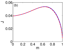
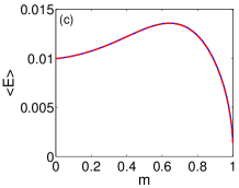
Figure 6: Action $J$ [Eq. (IV)] (top panels) and average energy $<E>$ [Eq. (IV)] (bottom panels) of solutions of the linear oscillator [Eq. (10)] vs shape parameter $m$ for the complete Fourier series (solid lines) of excitation (3) and the main harmonic approximation ($G_{2k+1}=0\ \forall k\geq 1$; dashed lines) and two sets of parameters: (left panels) $\omega_{\mathrm{b}}=0.8$, $f_{0}=0.02$, $\alpha=0.02$. (right panels) $\omega_{\mathrm{b}}=5$, $f_{0}=3$, $\alpha=0.1$.

As already anticipated in Sec. I, threshold phenomena associated with breathers’ emergence and stability exhibit a high sensitivity to the excitation’s impulse. To show this, we start with a general argument showing the relationship between energy changes and the quantities action and impulse for periodic solutions of isolated (nonlinear) oscillators. After integrating the corresponding energy equation over half a period (see, e.g., 6 ; 7 ), one obtains

$$\Delta E\equiv E(T/2)-E(0)=-\alpha\int_{0}^{T/2}\left(\dot{u}^{2}(t)\right)\mathrm{d}t+\int_{0}^{T/2}\dot{u}(t)F(t)\mathrm{d}t.$$ (18)

Now, after applying the first mean value theorem for integrals GR to the last integral on the right-hand side of Eq. (IV) and recalling the definitions of action and impulse, one obtains

$$\Delta E=-\alpha\pi J+T\dot{u}(t^{\ast})I,$$ (19)

where $t^{\ast}\in[0,T/2]$ while $J$ and $I$ are the action and the impulse, respectively. Note that $t^{\ast}$ becomes independent of the excitation’s waveform as $T\rightarrow 0$ 6 ; 7 . It should be stressed that this limiting regime is unreachable for the present case of discrete breathers in nonlinear chains, specially in the soft potential case, due to breather frequencies are always below a maximum, and hence they cannot be increased arbitrarily. Therefore, we see that the dependence of $\Delta E$ on $m$ for any (linear or nonlinear) isolated oscillator relies on the dependence on $m$ of $J$ and $\dot{u}(t^{\ast})I$. For the case of a linear oscillator and the excitation $f_{1}(t)$ (3), one readily obtains that $\dot{u}(t^{\ast})I$ can be expressed as $\sum_{k}\mu_{2k+1}^{(1)}G_{2k+1}^{2}$, where $\mu_{k}^{(1)}$ is independent on $m$, and hence the energy will present a maximum at $m=m_{\ell}^{\prime}\approx m_{\ell}$. We find that the dependence of the action on the shape parameter for nonlinear oscillators is quite similar to that of the discussed linear case.

To connect this analysis of isolated oscillators with discrete breathers of nonlinear chains (1), one has to calculate the action of a breather, $J=\sum_{n}\oint\dot{u}_{n}\mathrm{d}u_{n}$, on the one hand, and to distinguish between the periodic attractors with large and the small amplitudes, on the other hand, since the orbits associated with the latter can substantially differ from those of a strictly linear oscillator despite of its relatively small oscillation amplitude. In any case, numerical simulations confirmed that the value $m=m_{\max}\approx 0.717$ at which the impulse function $I_{1}(m)$ presents a single maximum is very close to $m_{\ell}$ in the sense that the waveforms corresponding to $m_{\max}$ and $m_{\ell}$ (and $m_{1}$) can be hardly distinguishable. Figure 7 shows an illustrative example for the cases of a hard $\phi^{4}$ potential and a sine-Gordon potential, while Fig. 8 shows, for the case of a hard $\phi^{4}$ potential, that the breather action presents a single maximum at $m=m_{b,\max}$ which is also very close to $m_{\ell}\approx 0.646$.

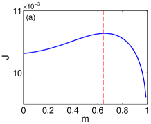
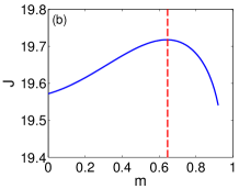
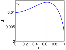
Figure 7: Action $J$ of (top panels) large-amplitude attractors and (bottom panels) small-amplitude attractors corresponding to an isolated nonlinear oscillator with (left panels) a sine-Gordon potential for the excitation (3), $\omega_{\mathrm{b}}=0.8$, $f_{0}=0.02$, $\alpha=0.02$, and (right panels) a $\phi^{4}$ potential for $\omega_{\mathrm{b}}=5$, $f_{0}=3$, $\alpha=0.1$. The vertical dashed lines indicate the $m$ value where the action of the linear oscillator is maximum, i.e. $m=m_{\ell}$ (cf. Fig. 6).

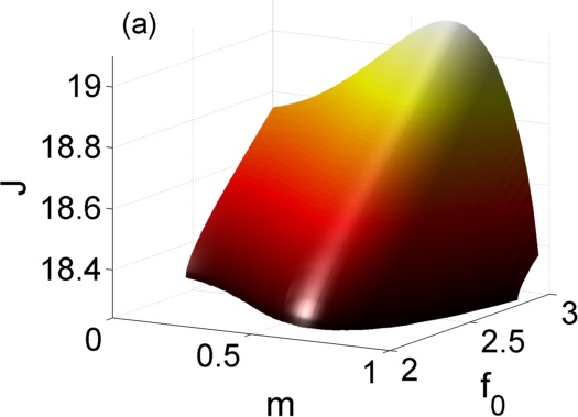
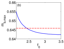
Figure 8: (a) Action $J$ of a breather emerging in a $\phi^{4}$ chain vs $f_{0}$ and $m$ in the range $f_{0}\in(2.06,3)$ for the excitation (3). (b) Shape parameter value at which the action is maximum $m_{b,\max}$ vs amplitude $f_{0}$; horizontal line corresponds to $m=m_{\ell}=0.646$. Fixed parameters: $\omega_{\mathrm{b}}=5$, $\alpha=0.1,$ $C=1$.

V Conclusions

We have shown through the example of a discrete nonlinear Klein-Gordon equation that varying the impulse transmitted by periodic external excitations is a universal procedure to reliably control the generation of stationary and moving discrete breathers in driven dissipative chains capable of presenting these intrinsic localized modes. We have analytically demonstrated that the enhancer effect of the excitation’s impulse, in the sense of facilitating the generation of stationary and moving breathers, is due to a correlative increase of the breather’s action, while numerical experiments corresponding to the cases of a hard $\phi^{4}$ potential and a sine-Gordon potential confirmed the effectiveness of the impulse as the relevant quantity controlling the effect of the external excitation. The consideration of this relevant quantity opens up new avenues for studying external-excitation-induced phenomena involving intrinsic localized modes in discrete nonlinear systems, including, for instance, breather-to-soliton transitions and emergence of chaotic breathers. Our present work is aimed to explore these and related problems.

- (1) S. Aubry. Physica D 103, 201 (1997); S. Flach and C. R. Willis. Phys. Rep. 295, 181 (1998); S. Flach and A. V. Gorbach. Phys. Rep. 467, 1 (2008).
- (2) S. Aubry. Physica D 216, 1 (2006);
- (3) E. Trías, J. J. Mazo and T. P. Orlando. Phys. Rev. Lett. 84, 741 (2000). P. Binder, D. Abraimov, A. V. Ustinov, S. Flach and Y. Zolotaryuk, Phys. Rev. Lett. 84, 745 (2000).
- (4) J. Cuevas, L. Q. English, P. G. Kevrekidis, M. Anderson, Phys. Rev. Lett. 102, 224101 (2009); V. J. Sánchez-Morcillo, N. Jiménez, J. Chaline, A. Bouakaz, and S. Dos Santos, in Localized Excitations in Nonlinear Complex Systems (Springer International, Switzerland, 2014), pp. 251–262; J. Chaline, N. Jiménez, A. Mehrem, A. Bouakaz, S. Dos Santos and V. J. Sánchez-Morcillo. J. Ac. Soc. Am. 138, 3600 (2015).
- (5) M. Sato, B. E. Hubbard and A. J. Sievers. Rev. Mod. Phys. 78, 137 (2006); M. Kimura, T. Hikihara, Chaos 19, 013138 (2009).
- (6) N. Boechler, G. Theocharis, S. Job, P. G. Kevrekidis, M. Porter and C. Daraio. Phys. Rev. Lett. 104, 244302 (2010); G. James, P. G. Kevrekidis, and J. Cuevas. Physica D 251, 39 (2013).
- (7) L. Q. English, F. Palmero, A. J. Sievers, P. G. Kevrekidis, and D. H. Barnak. Phys. Rev. E 81, 046605 (2010); F. Palmero, L. Q. English, J. Cuevas, R. Carretero-González and P. G. Kevrekidis. Phys. Rev. E 84, 026605 (2011); L. Q. English, F. Palmero, P. Candiani, J. Cuevas, R. Carretero-González, P. G. Kevrekidis and A. J. Sievers. Phys. Rev. Lett., 108, 084101 (2012); L. Q. English, F. Palmero, J. F. Stormes, J. Cuevas, R. Carretero-González and P. G. Kevrekidis. Phys. Rev. E 88, 022912 (2013).
- (8) M. Peyrard, Nonlinearity 17, R1 (2004).
- (9) See, e.g., M. Alonso and E. J. Finn, Physics (Addison-Wesley, New York, 1992), p. 118.
- (10) R. Chacón, J. Phys. A 40, F413 (2007); 43, 322001 (2010); P. J. Martínez and R. Chacón, Phys. Rev. Lett. 100, 144101 (2008); M. Rietmann, R. Carretero-González, and R. Chacón, Phys. Rev. A 83, 053617 (2011).
- (11) R. Chacón, M. Yu. Uleysky, and D. V. Makarov, Europhys. Lett. 90, 40003 (2010).
- (12) R. Chacón, Phys. Rev. A 85, 013813 (2012).
- (13) M.-D. Wei and C.-C. Hsu, Opt. Commun. 285, 1366 (2012).
- (14) P. J. Martínez and R. Chacón, Phys. Rev. E 93, 042311 (2016).
- (15) R. Chacón, F. Palmero, and J. Cuevas-Maraver, Phys. Rev. E 93, 062210 (2016).
- (16) D. Cubero, J. Cuevas and P. G. Kevrekidis. Phys. Rev. Lett. 102, 205505 (2009).
- (17) J. L. Marín F. Falo, P. J. Martínez and L. M. Floría. Phys. Rev. E 63, 066603 (2001).
- (18) O. M. Braun, Yu. S. Kivshar, The Frenkel-Kontorova Model: Concepts, Methods and Applications (Springer-Verlag, Berlin, 1998)
- (19) M. Chirilus-Bruckner, C. Chong, J. Cuevas-Maraver and P. G. Kevrekidis. In J. Cuevas-Maraver, P. G. Kevrekidis and F. Williams (Eds.), The sine-Gordon model and its applications (Vol. 10, pp. 31–57). Springer International Publishing (2014)
- (20) S. Aubry and T. Cretegny. Physica D 119, 34 (1998).
- (21) R. S. MacKay and S. Aubry. Nonlinearity 7, 1623 (1994); J. L. Marín and S. Aubry. Nonlinearity 9, 1501 (1996).
- (22) P. J. Martínez, M. Meister, L. M. Floría and F. Falo. Chaos 13, 610 (2003).
- (23) S. Takeno and M. Peyrard. Physica D 92, 140 (1996).
- (24) M. Fečkan, M. Pospíšil, V.M. Rothos and H. Susanto. J. Dyn. Diff. Equat. 25, 795 (2013).
- (25) R. S. MacKay and J.-A. Sepulchre. Physica D 119, 148 (1998); J. L. Marín, S. Aubry and L. M. Floría. Physica D 113,283 (1998).
- (26) I. S. Gradshteyn and I. M. Ryzhik, Table of Integrals, Series, and Products (Academic Press, San Diego, 1980).