Imaging in random media with convex optimization

Abstract

We study an inverse problem for the wave equation where localized wave sources in random scattering media are to be determined from time resolved measurements of the waves at an array of receivers. The sources are far from the array, so the measurements are affected by cumulative scattering in the medium, but they are not further than a transport mean free path, which is the length scale characteristic of the onset of wave diffusion that prohibits coherent imaging. The inversion is based on the Coherent Interferometric (CINT) imaging method which mitigates the scattering effects by introducing an appropriate smoothing operation in the image formation. This smoothing stabilizes statistically the images, at the expense of their resolution. We complement the CINT method with a convex ($l_{1}$) optimization in order to improve the source localization and obtain quantitative estimates of the source intensities. We analyze the method in a regime where scattering can be modeled by large random wavefront distortions, and quantify the accuracy of the inversion in terms of the spatial separation of individual sources or clusters of sources. The theoretical predictions are demonstrated with numerical simulations.

today

1 Introduction

Waves measured by a collection of nearby sensors, called an array of receivers, carry information about their source and the medium through which they travel. We consider a typical remote sensing regime with sources of small (point-like) support, and study the inverse problem of determining them from the array measurements.

When the waves travel in a known and non-scattering (e.g. homogeneous) medium, the sources can be localized with reverse time migration [4, 5] also known as backprojection [20]. This estimates the source locations as the peaks of the image formed by superposing the array recordings delayed by travel times from the receivers to the imaging points. The accuracy of the estimates depends on the array aperture, the distance of the sources from the array, and the temporal support of the signals emitted by the sources. It may be improved under certain conditions by using $l_{1}$ optimization, which seeks to invert the linear mapping from supposedly sparse vectors of the discretized source amplitude on some mesh, to the array measurements. The fast growing literature of imaging with $l_{1}$ optimization in homogeneous media includes compressed sensing studies such as [19, 18], synthetic radar imaging studies like [1, 8], array imaging studies like [14], and the resolution study [7].

In this paper we assume that the waves travel in heterogeneous media with fluctuations of the wave speed caused by numerous inhomogeneities. The amplitude of the fluctuations is small, meaning that a single inhomogeneity is a weak scatterer. However, there are many inhomogeneities that interact with the waves on their way from the sources to the receivers, and their scattering effect accumulates. Because in applications it is impossible to know the inhomogeneities in detail, and these cannot be estimated from the array measurements as part of the inversion, the fluctuations of the wave speed are uncertain. We model this uncertainty with a random process, and thus study inversion in random media. In this stochastic framework, the actual heterogeneous medium in which the waves propagate is one realization of the random model. The data measured at the array are uncertain and the question is how to mitigate the uncertainty to get images that are robust with respect to arbitrary medium realizations, i.e., they are statistically stable.

The mitigation of uncertainty in the wave propagation model becomes important when the sources are further than a few scattering mean free paths from the array. The scattering mean free path is the length scale on which the waves randomize [23], meaning that their fluctuations from one medium realization to another are large in comparison with their coherent (statistical expectation) part. The random wave distortions registered at the array are very different from additive and uncorrelated noise assumed usually in inversion. They are more difficult to mitigate and lead to poor and unreliable source reconstructions by coherent methods like reverse time migration or standard $l_{1}$ optimization. The Coherent Interferometric (CINT) method [9, 6] is designed to deal efficiently with such random distortions, as long as there is some residual coherence in the array measurements. This holds when the sources are separated from the array by distances (ranges) that are large with respect to the scattering mean free path, but do not exceed a transport mean free path, which is the distance at which the waves forget their initial direction [23]. The transport mean free path defines the range limit of applicability of coherent inversion methods. Beyond it only incoherent methods based on transport or diffusion equations [2] can be used.

In this paper we assume a scattering regime where the CINT method is useful. It forms images by superposing cross-correlations of the array measurements, delayed by travel times between the receivers and the imaging points. As shown in [9, 10, 6], the cross-correlations must be computed locally, in appropriate time windows, and over limited receiver offsets. This introduces a smoothing in the CINT image formation, which is essential for stabilizing statistically the images, at the expense of resolution. The larger the random distortions of the array measurements, the more smoothing is needed and the worse the resolution [9, 10]. Thus, it is natural to ask if it is possible to improve the source localization by using the prior information that the sources have small support.

We show that under generic conditions, the CINT imaging function is approximately a discrete convolution of the vector of source intensities discretized on the imaging mesh, with a blurring kernel. To reconstruct the sources we seek to undo the convolution using convex ($l_{1}$) optimization. We present an analysis of the method in a scattering regime where the random medium effects on the array measurements can be modeled by large wavefront distortions, as assumed in adaptive optics [3]. We derive from first principles the CINT blurring kernel in this regime, and state the inversion problem as an $l_{1}$ optimization. We also quantify the quality of the reconstruction with error estimates that depend on the separation of the sources, or of clusters of sources, but are independent of the source placement on or off the imaging mesh, as long as the sources are sufficiently far apart. The analysis shows that we can expect almost exact reconstructions when the sources are further apart than the CINT resolution limits. This is similar to the super-resolution results in [11], that show that one dimensional discrete convolutions can be undone by convex optimization, assuming that the minimum distance between the points in the support of the unknown vectors is $2/f_{c}$, where $f_{c}$ is the largest “frequency” in the Fourier transform of the convolution kernel. When the sources are clustered together, the $l_{1}$ reconstruction is not guaranteed to be close to the true vector of source intensities in the point-wise sense. However, we show that its support is in the vicinity of the clusters, and its entries are related to the average source intensities there.

The paper is organized as follows: We begin in section 2 with the formulation of the inverse problem as an $l_{1}$ optimization. The analysis of the method is in sections 3 - 5, and we demonstrate its performance with numerical simulations in section 6. We end with a summary in section 7.

2 Formulation of the inverse problem

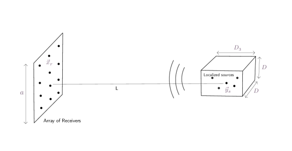
Fig. 1: Schematic for the inversion setup with an array of receivers that is planar square of side $a$. The range direction is orthogonal to the array aperture. The sources are at ranges of order $L$ in an imaging region $\mathfrak{D}$ modeled as a rectangular prism with size $D_{3}$ in range and $D$ in cross-range.

Consider the inversion setup illustrated in Figure 1, where $N_{s}$ sources located at $\vec{\bm{y}}_{s}$, for $s=1,\ldots,N_{s}$, emit signals $f_{s}(t)$ that generate sound waves recorded at a remote array of receivers placed at $\vec{\bm{x}}_{r}$, for $r=1,\ldots,N_{r}$. For simplicity we assume that the array aperture is planar and square, of side $a$. This allows us to introduce a system of coordinates centered at the array, with range direction orthogonal to the array, and cross-range plane parallel to the array. In this system of coordinates we have $\vec{\bm{x}}_{r}=(\bm{x}_{r},0)$, with cross-range vectors $\bm{x}_{r}=(x_{r,1},x_{r,2})$ satisfying $|x_{r,1}|,|x_{r,2}|\leq a/2$. The sources are at $\vec{\bm{y}}_{s}=(\bm{y}_{s},y_{s,3})$, with range coordinates $y_{s,3}$ of order $L$, satisfying $L\gg a$, and two dimensional cross-range vectors $\bm{y}_{s}$.

In general, the signals $f_{s}(t)$ emitted by the sources may be pulses, chirps or even noise-like, with Fourier transforms

$$\widehat{f}_{s}(\omega)=\int_{-\infty}^{\infty}dt\,f_{s}(t)e^{i\omega t}$$ (1)

supported in the frequency interval $[\omega_{o}-\pi B,\omega_{o}+\pi B]$, where $\omega_{o}$ is the central frequency and $B$ is the bandwidth. We denote the recorded waves by $p(\vec{\bm{x}}_{r},t)$, and use the linearity of the wave equation to write

$$p(\vec{\bm{x}}_{r},t)=\int_{\omega_{o}-\pi B}^{\omega_{o}+\pi B}\frac{d\omega}{2\pi}\,\widehat{p}(\vec{\bm{x}}_{r},\omega)e^{-i\omega t},\qquad\widehat{p}(\vec{\bm{x}}_{r},\omega)=\sum_{s=1}^{N_{s}}\widehat{f}_{s}(\omega)\widehat{G}(\vec{\bm{x}}_{r},\vec{\bm{y}}_{s},\omega)+\widehat{n}(\vec{\bm{x}}_{r},\omega),$$ (2)

for $r=1,\ldots,N_{r}$. Here the Green’s function $\widehat{G}$ models the propagation of time harmonic waves in the medium, and $\widehat{n}$ denotes additive and uncorrelated noise. The inverse problem is to determine the sources from these array measurements.

2.1 Imaging in homogeneous media

The Green’s function in media with constant speed $c_{o}$ is

$$\widehat{G}_{o}(\vec{\bm{x}}_{r},\vec{\bm{y}}_{s},\omega)=\frac{\exp[i\omega\tau(\vec{\bm{x}}_{r},\vec{\bm{y}}_{s})]}{4\pi|\vec{\bm{x}}_{r}-\vec{\bm{y}}_{s}|},$$ (3)

where

$$\tau(\vec{\bm{x}}_{r},\vec{\bm{y}}_{s})={|\vec{\bm{x}}_{r}-\vec{\bm{y}}_{s}|}/{c_{o}}$$ (4)

is the travel time from the source at $\vec{\bm{y}}_{s}$ to the receiver at $\vec{\bm{x}}_{r}$. The measurements are of the form

$$p_{o}(\vec{\bm{x}}_{r},t)=\sum_{s=1}^{N_{s}}\frac{f_{s}\left(t-\tau(\vec{\bm{x}}_{r},\vec{\bm{y}}_{s})\right)}{4\pi|\vec{\bm{x}}_{r}-\vec{\bm{y}}_{s}|}+n(\vec{\bm{x}}_{r},t),$$ (5)

and in reverse time migration they are synchronized using travel time delays with respect to a presumed source location at a search point $\vec{\bm{y}}$, and then superposed to form an image

$$\mathcal{J}_{o}(\vec{\bm{y}})=\sum_{r=1}^{N_{r}}p_{o}\left(\vec{\bm{x}}_{r},\tau(\vec{\bm{x}}_{r},\vec{\bm{y}})\right).$$ (6)

The resolution limits of the imaging function (6) are well known. The cross-range resolution is of order $\lambda_{o}L/a$, where $\lambda_{o}=2\pi c_{o}/\omega_{o}$ is the central wavelength, and the range resolution is inverse proportional to the temporal support of $f_{s}(t)$, which determines the precision of the travel time estimation. If the signals $f_{s}(t)$ are pulses, their temporal support is of order $1/B$, and the range resolution is of order $c_{o}/B$. If they are chirps or other long signals that are known, then they must be compressed in time by cross-correlation (matched filtering) with the time reversed $f_{s}(t)$ to achieve the $c_{o}/B$ range resolution [15]. If the signals are unknown and noise-like, then imaging must be based on cross-correlations of the array measurements, like in CINT.

We refer to [7] for the formulation of the inverse source problem as an $l_{1}$ optimization, and recall from there that the resolution limits $\lambda_{o}L/a$ and $c_{o}/B$ also play a role in the successful recovery of the presumed sparse source support.

2.2 Coherent interferometric imaging

The imaging function $\mathcal{J}_{o}(\vec{\bm{y}})$ does not work well in random media at ranges $L$ that exceed a few scattering mean free paths. This is because the measurements have large random distortions that are very different than the additive noise $n(\vec{\bm{x}}_{r},t)$, and cannot be reduced by simply summing over the receivers as in (6). To mitigate these distortions we image with the CINT function

$$\mathcal{J}(\vec{\bm{y}})=\int_{-\infty}^{\infty}d\omega\int_{-\infty}^{\infty}d\widetilde{\omega}\,\widehat{\phi}\left(\frac{\widetilde{\omega}}{\Omega}\right)\sum_{r=1}^{N_{r}}\sum_{r^{\prime}=1}^{N_{r}}\psi\left(\frac{|\bm{x}_{r}-\bm{x}_{r^{\prime}}|}{X(\omega)}\right)\widehat{p}(\vec{\bm{x}}_{r},\omega+\widetilde{\omega}/2)\overline{\widehat{p}(\vec{\bm{x}}_{r^{\prime}},\omega-\widetilde{\omega}/2)}$$

$$\times\exp[-i(\omega+\widetilde{\omega}/2)\tau(\vec{\bm{x}}_{r},\vec{\bm{y}})+i(\omega-\widetilde{\omega}/2)\tau(\vec{\bm{x}}_{r^{\prime}},\vec{\bm{y}})],$$ (7)

where $\widehat{\phi}$ and $\psi$ are smooth window functions of dimensionless argument and support of order one, and the domain of integration is restricted by the finite bandwidth that supports the measurements,

$$\omega\pm\widetilde{\omega}/2\in[\omega_{o}-\pi B,\omega_{o}+\pi B].$$

As in reverse time migration, the travel times are used in (7) to synchronize the waves due to a presumed source at the search location $\vec{\bm{y}}$. However, the image is formed by superposing cross-correlations of the array measurements $p(\vec{\bm{x}}_{r},t)$, instead of the measurements themselves. The cross-correlations are convolutions of $p(\vec{\bm{x}}_{r},t)$ with the time reversed $p(\vec{\bm{x}}_{r^{\prime}},t)$, for $r,r^{\prime}=1,\ldots,N_{r}$. The time reversal appears as complex conjugation in the frequency domain, denoted with the bar in (7). The time window

$$\phi\left(\Omega t\right)=\frac{1}{2\pi\Omega}\int_{-\infty}^{\infty}d\omega\,\widehat{\phi}\left(\frac{\omega}{\Omega}\right)e^{-i\omega t}$$ (8)

and spatial window $\psi(|\bm{x}|/X)$ ensure that the cross-correlations are computed locally, over receiver offsets that do not exceed the distance $X$, and over time offsets of order $1/\Omega$. These threshold parameters account for the fact that scattering in random media decorrelates statistically the waves at frequencies separated by more than $\Omega_{d}$, the decoherence frequency, and points separated by more than $X_{d}$, the decoherence length. We refer to [10, 6] and the next section for more details. Here it suffices to recall that (7) is robust when $X\lesssim X_{d}$ and $\Omega\lesssim\Omega_{d}$, and that the image $\mathcal{J}(\vec{\bm{y}})$ has a cross-range resolution of order $\lambda_{o}L/X$ and a range resolution of order $c_{o}/\Omega$. The best focus occurs at $X\approx X_{d}$ and $\Omega\approx\Omega_{d}$, so the decoherence parameters $X_{d}$ and $\Omega_{d}$ can be estimated with optimization, as explained in [9].

To state the inverse problem as a convex optimization, we make the simplifying assumption that the sources emit the same known pulse $f(t)$, so that

$$\widehat{f}_{s}(\omega)=\widehat{f}(\omega)\rho(\vec{\bm{y}}_{s}),\qquad s=1,\ldots,N_{s},$$ (9)

for an unknown, complex valued amplitude $\rho(\vec{\bm{y}})$. Using (9) in (2) and substituting in (7) we obtain

$$\mathcal{J}(\vec{\bm{y}})\approx\sum_{s=1}^{N_{s}}\sum_{s^{\prime}=1}^{N_{s}}\rho(\vec{\bm{y}}_{s})\overline{\rho(\vec{\bm{y}}_{s^{\prime}})}\,\kappa(\vec{\bm{y}},\vec{\bm{y}}_{s},\vec{\bm{y}}_{s^{\prime}}),$$ (10)

with kernel

$$\kappa(\vec{\bm{y}},\vec{\bm{y}}_{s},\vec{\bm{y}}_{s^{\prime}})= \sum_{r=1}^{N_{r}}\sum_{r^{\prime}=1}^{N_{r}}\psi\left(\frac{|\bm{x}_{r}-\bm{x}_{r^{\prime}}|}{X}\right)\int_{-\infty}^{\infty}d\omega\int_{-\infty}^{\infty}d\widetilde{\omega}\,\widehat{\phi}\left(\frac{\widetilde{\omega}}{\Omega}\right)\widehat{f}\left(\omega+{\widetilde{\omega}}/{2}\right)\overline{\widehat{f}\left(\omega-{\widetilde{\omega}}/{2}\right)}$$

$$\times\widehat{G}\left(\vec{\bm{x}}_{r},\vec{\bm{y}}_{s},\omega+{\widetilde{\omega}}/{2}\right)\overline{\widehat{G}(\vec{\bm{x}}_{r^{\prime}},\vec{\bm{y}}_{s^{\prime}},\omega-\widetilde{\omega}/2)}\exp[-i(\omega+\widetilde{\omega}/2)\tau(\vec{\bm{x}}_{r},\vec{\bm{y}})]+i(\omega-\widetilde{\omega}/2)\tau(\vec{\bm{x}}_{r^{\prime}},\vec{\bm{y}})],$$ (11)

where the approximation is because we neglect the additive noise.

In the analysis of the next section we take the Gaussian pulse

$$\widehat{f}(\omega)=\left(\frac{\sqrt{2\pi}}{B}\right)^{1/2}\exp\left[-\frac{(\omega-\omega_{o})^{2}}{4B^{2}}\right],$$ (12)

normalized by

$$\|f\|_{{}_{2}}=\left[\int_{-\infty}^{\infty}dt\,|f(t)|^{2}\right]^{1/2}=\left[\int_{-\infty}^{\infty}\frac{d\omega}{2\pi}\,|\widehat{f}(\omega)|^{2}\right]^{1/2}=1.$$

This choice allows us to obtain an explicit expression of the kernel (11). Naturally, in practice the pulses may not be Gaussian, and the sources may emit different signals. The method described here still applies to such cases, with $\rho(\vec{\bm{y}}_{s})$ replaced in (10) by $\|f_{s}\|_{{}_{2}}$, and the substitution

$$\widehat{f}(\omega+\widetilde{\omega}/2)\overline{\widehat{f}(\omega-\widetilde{\omega}/2)}\leadsto\frac{\widehat{f}_{s}(\omega+\widetilde{\omega}/2)}{\|f_{s}\|}\frac{\overline{\widehat{f}_{s^{\prime}}(\omega-\widetilde{\omega}/2)}}{\|f_{s^{\prime}}\|_{{}_{2}}}$$

in (11). Since $f_{s}$ is unknown in general, we may only estimate the kernel $\kappa$ up to unknown, constant multiplicative factors. This still allows the determination of the location of the sources, but does not give good estimates of their intensities.

2.3 The optimization problem

Let us consider a reconstruction mesh with $N_{z}$ points denoted generically by $\vec{\bm{z}}$, and name $\bm{\rho}$ the column vector with entries given by the unknown $\rho(\vec{\bm{z}})$. We sample the CINT image $\mathcal{J}(\vec{\bm{y}})$ at $N_{y}<N_{z}$ points, and gather these samples in the “data” vector $\bm{d}$. It is natural to take $N_{y}<N_{z}$, because we seek to super-resolve the CINT image, which is blurred by the kernel (51).

At first glance it appears that we may use equation (10) to formulate the inversion as an optimization problem for recovering the rank one matrix $\bm{\rho}\bm{\rho}^{\star}$, as in [12, 13]. However, as shown in the next section, in strong random media where CINT is needed, the kernel $\kappa(\vec{\bm{y}},\vec{\bm{z}},\vec{\bm{z}}^{\prime})$ is large only when $\vec{\bm{z}}$ and $\vec{\bm{z}}^{\prime}$ are nearby. In fact, for reasonable mesh sizes on which we can expect to obtain unique reconstructions, the kernel satisfies

$$\kappa(\vec{\bm{y}},\vec{\bm{z}},\vec{\bm{z}}^{\prime})\approx\left\{\begin{array}[]{ll}\kappa(\vec{\bm{y}},\vec{\bm{z}},\vec{\bm{z}})&\mbox{if}~{}\vec{\bm{z}}^{\prime}=\vec{\bm{z}},\\ 0&\mbox{if}~{}\vec{\bm{z}}\neq\vec{\bm{z}}^{\prime}.\end{array}\right.$$ (13)

Thus, only the diagonal entries $|\rho(\vec{\bm{z}})|^{2}$ of $\bm{\rho}\bm{\rho}^{\star}$ play a role. These are the source intensities and we denote by $\bm{u}\in\mathbb{R}^{N_{z}}$ the vector of unknowns formed by them. Equation (10) gives

$$\bm{\mathcal{M}}\,\bm{u}\approx\bm{d},$$ (14)

where $\bm{\mathcal{M}}$ is the $N_{y}\times N_{z}$ “measurement” matrix with entries $\kappa(\vec{\bm{y}},\vec{\bm{z}},\vec{\bm{z}}).$ We formulate the inversion as the $l_{1}$ optimization problem

$$\min_{\bm{u}\in\mathbb{R}^{N_{z}}}\|\bm{u}\|_{{}_{1}}~{}~{}\mbox{such that}~{}~{}\|\bm{\mathcal{M}}\,\bm{u}-\bm{d}\|_{{}_{2}}\leq~{}\mbox{tolerance},$$ (15)

where the tolerance accounts for additive noise effects and the random fluctuations of the CINT imaging function, which are small for large enough array aperture $a$ and bandwidth $B$, as shown in [10, 6].

We prove in section 4 that the left hand side in (14) is approximately a discrete convolution. The $l_{1}$ optimization is useful in this context, and recovers well sources that are well separated, as expected from the results in [11]. We rediscover such results in this paper using a different analysis. We also consider cases where the sources are clustered together, and show that although we cannot expect good reconstructions in the point-wise sense, the $l_{1}$ minimizer is supported in the vicinity of the clusters, and estimates the average source intensity there.

3 Setup of the analysis

We introduce in this section the random wave speed model and the scaling assumptions which define the relations between the wavelength $\lambda_{o}$, the typical size $\ell$ of the inhomogeneities in the medium, the standard deviation $\sigma$ of the fluctuations of the wave speed, the array aperture $a$, the range $L$, and the extent of the imaging region. The scaling allows us to describe the scattering effects of the random medium as large wavefront distortions. This is a simple wave propagation model that is convenient for analysis, and captures qualitatively all the important features of imaging with CINT. That is to say, equation (14) holds in general scattering regimes, and the CINT kernel $\kappa$ has a similar form, but the mathematical expression of the decoherence length $X_{d}$ and frequency $\Omega_{d}$, which quantify the blurring by the kernel, are expected to change. The expressions of $X_{d}$ and $\Omega_{d}$ in terms of $\lambda_{o},\sigma,\ell$ and $L$ are needed for analysis, but they are unlikely to be known in practice. This is why one should determine the decoherence parameters directly form the data or adaptively, during the CINT image formation, as in [9].

The model of the wave speed $c(\vec{\bm{x}})$ is

$$c(\vec{\bm{x}})=c_{o}\left[1+\sigma\mu\left(\frac{\vec{\bm{x}}}{\ell}\right)\right]^{-1/2},$$ (16)

where $\mu$ is a mean zero, stationary random process of dimensionless argument. We suppose that $\mu$ is bounded almost surely and denote by $\mathcal{R}$ its auto-correlation, assumed isotropic and Gaussian for convenience

$$\mathcal{R}(\vec{\bm{x}})=\mathbb{E}\left[\mu(\vec{\bm{x}}+\vec{\bm{x}}^{\prime})\mu(\vec{\bm{x}})\right]=e^{-|\vec{\bm{x}}|^{2}/2}.$$ (17)

Then, $\sigma\ll 1$ quantifies the small amplitude of the fluctuations of $c(\vec{\bm{x}})$, and $\ell$ is the correlation length, which characterizes the typical size of the inhomogeneities in the medium.

We explain in section 3.1 how far the waves should propagate in media modeled by (16), so that the cumulative scattering effects can be described by large wavefront distortions. We are interested in imaging with finite size arrays at long distances, so the waves propagate in the range direction, within a cone (beam) of small opening angle. This is the paraxial regime defined in section 3.2. We describe in section 3.3 the wave randomization quantified by the scattering mean free path, and the statistical decorrelation quantified by the decoherence length and frequency. We end the section with a summary of the scaling assumptions.

3.1 Wave scattering regime

We use a geometrical optics (Rytov) wave propagation model that holds in high frequency regimes with separation of scales

$$\lambda_{o}\ll\ell\ll L,$$ (18)

and standard deviation $\sigma$ of the fluctuations satisfying

$$\sigma\ll\min\left\{\left(\frac{\ell}{L}\right)^{3/2},\frac{\sqrt{\ell\lambda_{o}}}{L}\right\}.$$ (19)

It is shown in [22] that the first bound in (19) ensures that the rays remain straight and the variance of the amplitude of the Green’s function is negligible, so we can use the same geometrical spreading factor as in the homogeneous medium. The second bound in (19) ensures that only first order (in $\sigma$) corrections of the travel time matter, so the propagation model is

$$\widehat{G}(\vec{\bm{x}},\vec{\bm{y}},\omega)\approx\widehat{G}_{o}(\vec{\bm{x}},\vec{\bm{y}},\omega)\exp\left[i\omega\tau(\vec{\bm{x}},\vec{\bm{y}})\frac{\sigma}{2}\int_{0}^{1}d\vartheta\,\mu\left(\frac{(1-\vartheta)\vec{\bm{y}}+\vartheta\vec{\bm{x}}}{\ell}\right)\right].$$ (20)

Let us write the random phase correction in (20) as

$$\omega\delta\tau(\vec{\bm{x}},\vec{\bm{y}})=\frac{(2\pi)^{1/4}}{2}\sigma k\sqrt{\ell|\vec{\bm{x}}-\vec{\bm{y}}|}\,\nu(\vec{\bm{x}},\vec{\bm{y}}),$$ (21)

where $k=\omega/c_{o}$ is the wavenumber and

$$\nu(\vec{\bm{x}},\vec{\bm{y}})=\frac{1}{(2\pi)^{1/4}}\sqrt{\frac{|\vec{\bm{x}}-\vec{\bm{y}}|}{\ell}}\int_{0}^{1}d\vartheta\,\mu\left(\frac{(1-\vartheta)\vec{\bm{y}}+\vartheta\vec{\bm{x}}}{\ell}\right)$$ (22)

is defined by the integral of the fluctuations along the straight ray between $\vec{\bm{y}}$ and $\vec{\bm{x}}$. It is shown in [6, Lemma 3.1] that $\nu(\vec{\bm{x}},\vec{\bm{y}})$ converges in distribution as $\ell/|\vec{\bm{x}}-\vec{\bm{y}}|\sim\ell/L\to 0$ to a Gaussian process. Its mean

$$\mathbb{E}\left[\nu(\vec{\bm{x}},\vec{\bm{y}})\right]=0,$$ (23)

and variance

$$\mathbb{E}\left[\nu^{2}(\vec{\bm{x}},\vec{\bm{y}})\right]=\frac{|\vec{\bm{x}}-\vec{\bm{y}}|}{\ell\sqrt{2\pi}}\int_{0}^{1}d\vartheta\int_{0}^{1}d\vartheta^{\prime}\,\mathcal{R}\left(\frac{(\vartheta^{\prime}-\vartheta)(\vec{\bm{x}}-\vec{\bm{y}})}{\ell}\right)\approx 1,$$ (24)

are calculated from definition (22) and the expression (17) of $\mathcal{R}$. The approximation is for $\ell/L$ small.

We conclude from (21), (24) and $k=O(k_{o})$, with $k_{o}=2\pi/\lambda_{o}$, that the random phase fluctuations in (20) have standard deviation of order $\sigma\sqrt{\ell L}/\lambda_{o}$. When this is small, the random medium effects are negligible and any coherent imaging method works well. We are interested in the case of large fluctuations, so we ask that

$$\sigma\gg\frac{\lambda_{o}}{\sqrt{\ell L}}.$$ (25)

This is consistent with (19) when

$$\frac{\lambda_{o}/\sqrt{\ell L}}{(\ell/L)^{3/2}}=\frac{\lambda_{o}L}{\ell^{2}}\ll 1,\qquad\frac{\lambda_{o}/\sqrt{\ell L}}{\sqrt{\ell\lambda_{o}}/{L}}=\frac{\sqrt{\lambda_{o}L}}{\ell}\ll 1,$$

so we tighten our assumption (18) on the correlation length as

$$\sqrt{\lambda_{o}L}\ll\ell\ll L.$$ (26)

3.2 The paraxial regime

Suppose that the sources are contained in the search (imaging) region

$$\mathfrak{D}=\left[-D/2,D/2\right]\times\left[-D/2,D/2\right]\left[-D_{3}/2,D_{3}/2\right],$$ (27)

which is a rectangular prism of sides $D$ in cross-range and $D_{3}$ in range, as illustrated in Figure 1. When $D$ and the array aperture $a$ are small with respect to the range scale $L$, the rays connecting the sources and the receivers are contained within a cone (beam) of small opening angle, and we can use the paraxial approximation to simplify the calculations.

The paraxial regime is defined by the scaling relations

$$\lambda_{o}\ll D\lesssim a\ll L,\qquad D_{3}\ll L,\qquad\frac{a^{4}}{\lambda_{o}L^{3}}\ll 1,\qquad\frac{a^{2}D_{3}}{\lambda_{o}L^{2}}\ll 1,$$ (28)

so that for $\vec{\bm{y}}=(\bm{y},y_{3})$ and $\vec{\bm{x}}=(\bm{x},0)$ we get

$$k|\vec{\bm{x}}-\vec{\bm{y}}| =k\left(y_{3}+\frac{|\bm{x}|^{2}}{2L}-\frac{\bm{x}\cdot\bm{y}}{L}+\frac{|\bm{y}|^{2}}{2L}\right)+O\left(\frac{a^{4}}{\lambda_{o}L^{3}}\right)+O\left(\frac{a^{2}D_{3}}{\lambda_{o}L^{2}}\right)$$

$$\approx k\left(y_{3}+\frac{|\bm{x}|^{2}}{2L}-\frac{\bm{x}\cdot\bm{y}}{L}+\frac{|\bm{y}|^{2}}{2L}\right),$$ (29)

and

$$\frac{1}{4\pi|\vec{\bm{x}}-\vec{\bm{y}}|}=\frac{1}{4\pi L}\left[1+O\left(\frac{D_{3}}{L}\right)+O\left(\frac{a^{2}}{L^{2}}\right)\right]\approx\frac{1}{4\pi L}.$$ (30)

These approximations are proved in appendix A, and the deterministic factor in (20) becomes

$$\widehat{G}_{o}(\vec{\bm{x}},\vec{\bm{y}},\omega)\approx\frac{1}{4\pi L}\exp\left[ik\left(y_{3}+\frac{|\bm{x}|^{2}}{2L}-\frac{\bm{x}\cdot\bm{y}}{L}+\frac{|\bm{y}|^{2}}{2L}\right)\right].$$ (31)

3.3 Randomization and statistical decorrelation of the waves

Here we quantify the scattering mean free path $\mathcal{S}$, the length scale on which the waves randomize (lose coherence), and the decoherence length $X_{d}$ and frequency $\Omega_{d}$, which describe the statistical decorrelation of the waves due to scattering. These important scales appear in the definition of the CINT blurring kernel defined in section 4.

Proposition 1.

The expectation of the Green’s function (20) is given by

$$\mathbb{E}\big{[}\widehat{G}(\vec{\bm{x}},\vec{\bm{y}},\omega)\big{]}\approx\widehat{G}_{o}(\vec{\bm{x}},\vec{\bm{y}},\omega)e^{-\frac{|\vec{\bm{x}}-\vec{\bm{y}}|}{\mathcal{S}(\omega)}}\approx 0,$$ (32)

where $\mathcal{S}(\omega)$ is the scattering mean free path defined by

$$\mathcal{S}(\omega)=\frac{8}{\sqrt{2\pi}\sigma^{2}k^{2}\ell}\ll L.$$ (33)

This result, proved in appendix B, shows that the wavefront distortions due to scattering in the random medium do not average out. The expectation of $\widehat{G}$ is not the same as the Green’s function in the homogeneous medium, but decays exponentially with the distance of propagation on the scale $\mathcal{S}(\omega)$, the scattering mean free path. The scaling assumption (25) and definition (33) give

$$\frac{|\vec{\bm{x}}-\vec{\bm{y}}|}{\mathcal{S}(\omega)}=O\left(\frac{L}{\mathcal{S}(\omega)}\right)=O(\sigma^{2}k^{2}\ell L)\gg 1,$$

which is why the expectation in (32) is almost zero. The standard deviation of the fluctuations is approximately

$$\mbox{std}[\widehat{G}(\vec{\bm{x}},\vec{\bm{y}},\omega)]\approx\sqrt{\Big{|}\widehat{G}_{o}(\vec{\bm{x}},\vec{\bm{y}},\omega)\Big{|}^{2}-\Big{|}\mathbb{E}\big{[}\widehat{G}(\vec{\bm{x}},\vec{\bm{y}},\omega)\big{]}\Big{|}^{2}}\approx\Big{|}\widehat{G}_{o}(\vec{\bm{x}},\vec{\bm{y}},\omega)\Big{|},$$

where we used that $|\widehat{G}(\vec{\bm{x}},\vec{\bm{y}},\omega)|\approx|\widehat{G}_{o}(\vec{\bm{x}},\vec{\bm{y}},\omega)|$. Thus, the random fluctuations of the waves dominate their coherent part (the expectation) at the ranges considered in our analysis,

$$\frac{\Big{|}\mathbb{E}\big{[}\widehat{G}(\vec{\bm{x}},\vec{\bm{y}},\omega)\big{]}\Big{|}}{\mbox{std}[\widehat{G}(\vec{\bm{x}},\vec{\bm{y}},\omega)]}\approx e^{-\frac{|\vec{\bm{x}}-\vec{\bm{y}}|}{S(\omega)}}\approx 0,$$

and the wave is randomized. Reverse time migration or standard $l_{1}$ optimization methods cannot mitigate these large random distortions, as we illustrate with numerical simulations. This is why we base our inversion on the CINT method.

Proposition 2.

Consider two points $\vec{\bm{x}}=(\bm{x},0)$ and $\vec{\bm{x}}^{\prime}=(\bm{x}^{\prime},0)$ in the array aperture and two points $\vec{\bm{y}}=(\bm{y},y_{3})$ and $\vec{\bm{y}}^{\prime}=(\bm{y}^{\prime},y_{3}^{\prime})$ in the imaging region. Assume that the bandwidth $B$ is small with respect to the central frequency $\omega_{o}$, so that $|\omega-\omega_{o}|,|\omega^{\prime}-\omega_{o}|\leq\pi B\ll\omega_{o}$. Then, the second moments of (20) are

$$\mathbb{E}\left[\widehat{G}(\vec{\bm{x}},\vec{\bm{y}},\omega)\overline{\widehat{G}(\vec{\bm{x}}^{\prime},\vec{\bm{y}}^{\prime},\omega^{\prime})}\right]\approx\widehat{G}_{o}(\vec{\bm{x}},\vec{\bm{y}},\omega)\overline{\widehat{G}_{o}(\vec{\bm{x}}^{\prime},\vec{\bm{y}}^{\prime},\omega^{\prime})}e^{-\frac{|y_{3}-y_{3}^{\prime}|}{\mathcal{S}}-\frac{(\omega-\omega^{\prime})^{2}}{2\Omega_{d}^{2}}-\frac{|\bm{y}-\bm{y}^{\prime}|^{2}+(\bm{y}-\bm{y}^{\prime})\cdot(\bm{x}-\bm{x}^{\prime})+|\bm{x}-\bm{x}^{\prime}|^{2}}{2X_{d}^{2}}},$$ (34)

with short notation $\mathcal{S}=\mathcal{S}(\omega_{o})$, and decoherence frequency $\Omega_{d}$ and decoherence length $X_{d}$ defined by

$$\Omega_{d}=\frac{2\omega_{o}}{(2\pi)^{5/4}}\left(\frac{\lambda_{o}}{\sigma\sqrt{\ell L}}\right)\ll\omega_{o},\qquad X_{d}=\sqrt{3}\ell\,\frac{\Omega_{d}}{\omega_{o}}\ll\ell.$$ (35)

Moment formula (34) is proved in appendix B, and the inequalities in (35) are due to assumption (25). The first exponential factor in (34) accounts for the randomization due to the travel time fluctuations between the two ranges. In our scaling $|y_{3}-y_{3}^{\prime}|\lesssim D_{3}$, and by the last inequality in (28), and the definition of the scattering mean free path, we have

$$\frac{|y_{3}-y_{3}^{\prime}|}{\mathcal{S}(\omega_{o})}=O\left(D_{3}\frac{\sigma^{2}\ell}{\lambda_{o}^{2}}\right)\ll O\left(\frac{\lambda_{o}L^{2}}{a^{2}}\frac{\sigma^{2}\ell}{\lambda_{o}^{2}}\right)\ll O\left(\frac{\ell^{2}}{a^{2}}\right),$$ (36)

where we used the bound (19) on $\sigma$. It is shown in [6, Section 4] that the standard deviation of the CINT image is small with respect to the expectation of its peak value (i.e., the imaging function is statistically stable) when

$$a>\ell.$$ (37)

Stability is essential for imaging to succeed, so we ask that the array aperture satisfy (37), and conclude from (36) that the second moments (32) simplify as

$$\mathbb{E}\left[\widehat{G}(\vec{\bm{x}},\vec{\bm{y}},\omega)\overline{\widehat{G}(\vec{\bm{x}}^{\prime},\vec{\bm{y}}^{\prime},\omega^{\prime})}\right] \approx\widehat{G}_{o}(\vec{\bm{x}},\vec{\bm{y}},\omega)\overline{\widehat{G}_{o}(\vec{\bm{x}}^{\prime},\vec{\bm{y}}^{\prime},\omega^{\prime})}e^{-\frac{(\omega-\omega^{\prime})^{2}}{2\Omega_{d}^{2}}-\frac{|\bm{y}-\bm{y}^{\prime}|^{2}+(\bm{y}-\bm{y}^{\prime})\cdot(\bm{x}-\bm{x}^{\prime})+|\bm{x}-\bm{x}^{\prime}|^{2}}{2X_{d}^{2}}},$$ (38)

with $\widehat{G}_{o}$ given in (31).

The exponential decay in (38) models the statistical decorrelation of the waves due to scattering. In our context, the spatial decorrelation, modeled by the decay in $\bm{x}-\bm{x}^{\prime}$ and $\bm{y}-\bm{y}^{\prime}$, can be explained by the fact that rays connecting sources to far apart receivers traverse through different parts of the random medium. Because $\mu$ does not have long range correlations, the fluctuations of the travel time along such different rays are statistically uncorrelated. The waves at far apart frequencies are uncorrelated because they interact differently with the random medium. This gives the decay in $\omega-\omega^{\prime}$ in equation (38).

Definition (11) of the CINT kernel involves the superposition of $\widehat{G}(\vec{\bm{x}},\vec{\bm{y}},\omega)\overline{\widehat{G}(\vec{\bm{x}}^{\prime},\vec{\bm{y}}^{\prime},\omega^{\prime})}$ over the array elements and frequencies. If the array aperture $a$ is large with respect to $X_{d}$, the superposition stabilizes statistically because we sum many uncorrelated entries, as in the law of large numbers. This is why CINT is robust with respect to the uncertainty of the fluctuations of the wave speed, as shown in [10, 6].

3.4 Summary of the scaling assumptions

We gather here the scaling assumptions stated throughout the section, and complement them with extra assumptions on the bandwidth and the size of the imaging region. We refer to appendix C for the verification of their consistency.

The wavelength $\lambda_{o}$ is the smallest length scale, and the range $L$ is the largest. The assumptions (37) and (28) on the aperture are

$$\ell<a\ll(\lambda_{o}L^{3})^{1/4}.$$ (39)

The upper bound ensures that we can use the paraxial approximation and the lower bound gives $a>\ell\gg X_{d}$, so that the CINT image is statistically stable.

Assumption (26) combined with (39) gives that the correlation length of the wave speed fluctuations should satisfy

$$\sqrt{\lambda_{o}L}\ll\ell\ll(\lambda_{o}L^{3})^{1/4}\ll L.$$ (40)

The standard deviation $\sigma$ of the fluctuations is bounded above as in (19), and below as in (25),

$$\frac{\lambda_{o}}{\sqrt{\ell L}}\ll\sigma\ll\frac{\sqrt{\ell\lambda_{o}}}{L}.$$ (41)

The cross-range and range sizes $D$ and $D_{3}$ of the imaging region should be large with respect to the CINT resolution limits of $\lambda_{o}L/X$ in cross-range and $c_{o}/\Omega$ in range (see next section), so we can observe the image focus. We take the threshold parameters

$$X/X_{d}=O(1),\qquad\Omega/\min\{\Omega_{d},B\}=O(1),$$ (42)

and recalling the scaling assumptions (28) that allow us to use the paraxial approximation, we obtain

$$\frac{c_{o}}{\Omega}\ll D_{3}\ll\frac{\lambda_{o}L^{2}}{a^{2}}\quad\mbox{and}\quad\frac{\lambda_{o}L}{X}\ll D\lesssim a.$$ (43)

In general, the CINT image is statistically stable if in addition to having $a\gg X_{d}$, which follows from (35) and (39), the bandwidth $B$ is larger than the decoherence frequency $\Omega_{d}$. However, for the propagation model (20) considered in this section, where the effect of the random medium consists only of wavefront distortions and no delay spread (reverberations), the bandwidth $B$ does not play a role in the stabilization of CINT, as shown in [6, Section 4.4.4]. Thus, we study imaging in both narrowband and broadband regimes:

The narrowband regime is defined by $B$ satisfying

$$\omega_{o}\left(\frac{a}{L}\right)^{2}\ll B\ll\omega_{o}\min\left\{1,\frac{\lambda_{o}L}{aX_{d}}\right\}=\omega_{o}\frac{\lambda_{o}L}{aX_{d}}.$$ (44)

As verified in Appendix C,

$$\frac{\lambda_{o}L}{X_{d}}\ll\ell<a,\qquad\frac{\lambda_{o}L}{aX_{d}}\ll\frac{\Omega_{d}}{\omega_{o}},$$ (45)

so $B\ll\Omega_{d}$. This choice leads to a simpler expression of the CINT blurring kernel, but since $\Omega$ is of the order of $B$, the range resolution is the same as in the homogeneous medium, and cannot be improved with optimization unless the sources are very far apart in range. However, the optimization can improve the cross-range focusing.

The broadband regime is defined by

$$\Omega_{d}\ll B\ll\omega_{o},$$ (46)

so we may seek to improve the CINT resolution in both range and cross-range. The expression of the CINT kernel is more complicated in this case, but it simplifies slightly when

$$\frac{\lambda_{o}}{\sqrt{\ell L}}\ll\frac{\lambda_{o}^{2/3}\ell^{1/6}}{L^{5/6}}\ll\sigma\ll\frac{\sqrt{\ell\lambda_{o}}}{L},\qquad\frac{\ell}{a}=O(1).$$ (47)

We present the analysis that uses these conditions, which say that the fluctuations in the random medium are even stronger than in (41), but the correlation length is not much smaller than $a$. Extensions to larger apertures are possible, although the analysis is more complicated.

4 The CINT blurring kernel

Here we derive the CINT convolution model. To obtain an explicit expression of the kernel (11), we use the Gaussian pulse (12) and the Gaussian threshold windows

$$\widehat{\phi}\left(\frac{\widetilde{\omega}}{\Omega}\right)=e^{-\frac{\widetilde{\omega}^{2}}{2\Omega^{2}}},\qquad\psi\left(\frac{|\widetilde{\bm{x}}|}{X}\right)=e^{-\frac{|\widetilde{\bm{x}}|^{2}}{2\Omega^{2}}},$$ (48)

with $X$ and $\Omega$ satisfying

$${X}/{X_{d}}=O(1),\qquad\Omega=\left\{\begin{array}[]{ll}B&\mbox{in narrowband regime}\\ \\ O(\Omega_{d})&\mbox{in broadband regime}.\end{array}\right.$$ (49)

As stated previously, and shown in [9], $X_{d}$ and $\Omega_{d}$ can be estimated adaptively, by optimizing the focusing of the CINT image. This is why we can assume that $X_{d}$ is known approximately. The same holds for $\Omega_{d}$, if the bandwidth is big enough. The expression of the CINT kernel is simpler in the narrowband scaling (44), where $B\ll\Omega_{d}$, as shown in section 4.1, and we take $\Omega=B$. The broadband regime is discussed in section 4.2.

Typically, the receivers are separated by distances of order $\lambda_{o}$, so that they behave collectively as an array. Since $\lambda_{o}\ll a$, we have $N_{r}=O\left(a^{2}/\lambda_{o}^{2}\right)\gg 1,$ and we can approximate the sums in (11) by integrals

$$\sum_{r=1}^{N}\leadsto\frac{N_{r}}{a^{2}}\int_{\mathcal{A}}d\bm{x},$$

where $\mathcal{A}$ denotes the array aperture, the square of side $a$. To avoid specifying the finite aperture in the integrals, and to simplify the calculations, we use a Gaussian apodization factor

$$\psi_{\mathcal{A}}(\bm{x})=\exp\left[-\frac{|\bm{x}|^{2}}{2(a/6)^{2}}\right],$$ (50)

which is negligible outside the disk of radius $a/2$.

4.1 The CINT kernel in the narrowband regime

The calculation of the kernel (11) is in appendix D, and we state the results in the next proposition.

Proposition 3.

Let $\vec{\bm{z}}=(\bm{z},z_{3})$, $\vec{\bm{z}}^{\prime}=(\bm{z}^{\prime},z_{3}^{\prime})$ and $\vec{\bm{y}}=(\bm{y},y_{3})$ be three points in the imaging region and define the center and difference vectors

$$\frac{\vec{\bm{z}}+\vec{\bm{z}}^{\prime}}{2}=(\overline{\bm{z}},\overline{z}_{3}),\qquad\vec{\bm{z}}-\vec{\bm{z}}^{\prime}=(\widetilde{\bm{z}},\widetilde{z}_{3}).$$

Under the assumptions (39)-(44), the CINT kernel (11) is approximated by

$$\kappa(\vec{\bm{y}},\vec{\bm{z}},\vec{\bm{z}}^{\prime}) \approx C\exp\left[-\frac{|\overline{\bm{z}}-\bm{y}|^{2}}{2R^{2}}-\frac{(\overline{z}_{3}-y_{3})^{2}}{2R_{3}^{2}}\right]\,\mathfrak{M}(\vec{\bm{y}},\vec{\bm{z}},\vec{\bm{z}}^{\prime}),$$ (51)

where $C$ is a constant, and

$$R=\frac{L}{k_{o}X_{e}},\qquad R_{3}=\frac{c_{o}}{\Omega_{e}},$$ (52)

with $X_{e}$ and $\Omega_{e}$ defined by

$$\frac{1}{X_{e}^{2}}=\frac{1}{X_{d}^{2}}+\frac{1}{X^{2}}+\frac{1}{4(a/6)^{2}},\qquad\frac{1}{\Omega_{e}^{2}}=\frac{1}{\Omega_{d}^{2}}+\frac{1}{\Omega^{2}}+\frac{1}{4B^{2}}.$$ (53)

The factor $\mathfrak{M}(\vec{\bm{y}},\vec{\bm{z}},\vec{\bm{z}}^{\prime})$ is complex, with absolute value

$$|\mathfrak{M}(\vec{\bm{y}},\vec{\bm{z}},\vec{\bm{z}}^{\prime})|=\exp\left[-\frac{\widetilde{z}_{3}^{2}}{2\widetilde{R}^{2}}-\frac{|\widetilde{\bm{z}}|^{2}}{2}\left(\frac{1}{\gamma X_{d}^{2}}+\frac{1}{\widetilde{R}^{2}}\right)\right],$$ (54)

where

$$\frac{1}{\gamma}=1-\frac{X_{e}^{2}}{4X_{d}^{2}}>\frac{3}{4},\quad\widetilde{R}_{3}=\frac{c_{o}}{B},\quad\widetilde{R}=6\sqrt{2}\frac{L}{k_{o}a}.$$ (55)

The parameter $R$ defined in (52) is the CINT cross-range resolution limit, the length scale of exponential decay of the kernel $\kappa(\vec{\bm{y}},\vec{\bm{z}},\vec{\bm{z}}^{\prime})$ with $\overline{\bm{z}}-\bm{y}$. Definitions (53), (35) and assumption (49) give that

$$X_{e}=O(X_{d})\ll a,$$

so the resolution is worse than in homogeneous media,

$$R\gg\frac{L}{k_{o}a}.$$ (56)

This is due to the smoothing needed to stabilize statistically the image [9]. The goal of the convex optimization (15) is to overcome this blurring and localize better the sources in cross-range.

The parameter $R_{3}$ is the CINT range resolution limit. Because we are in the narrowband regime, we obtain from definition (53) and (49) that $\Omega_{e}\approx B,$ and therefore $R_{3}$ is similar to the range resolution in homogeneous media,

$$R_{3}=\frac{c_{o}}{\Omega_{e}}\approx\frac{c_{o}}{B}.$$ (57)

The results obtained in [7] for imaging with $l_{1}$ optimization in homogeneous media show that it is not possible to improve the $c_{o}/B$ range resolution, unless the sources are very far apart in range. We cannot expect to do better in random media, so we do not seek any super-resolution in range, in the narrowband regime.

Note that by the first inequality in (45) we have $\widetilde{R}\ll X_{d}$, so the kernel decays with the offsets $\widetilde{\bm{z}}$ and $\widetilde{z}$ on the length scales $\widetilde{R}$ and $\widetilde{R}_{3}$. These scales are, up to a constant of order one, the resolution limits of imaging in homogeneous media.

4.2 The CINT kernel in the broadband regime

The expression of the CINT kernel is stated in the next proposition, proved in appendix D.

Proposition 4.

Consider the same points and notation as in Proposition 3. Under the assumptions (39)-(43) and (46)-(47), the CINT kernel is given by

$$\kappa(\vec{\bm{y}},\vec{\bm{z}},\vec{\bm{z}}^{\prime}) \approx\frac{C}{\sqrt{1+\frac{|\overline{\bm{z}}-\bm{y}|^{2}}{2\theta^{2}R^{2}}}}\exp\left[-\frac{|\overline{\bm{z}}-\bm{y}|^{2}}{2R^{2}}-\frac{\big{(}\overline{z}_{3}-y_{3}+\frac{|\overline{\bm{z}}|^{2}-|\bm{y}|^{2}}{2L}\big{)}^{2}}{2R_{3}^{2}\big{[}1+\frac{|\overline{\bm{z}}-\bm{y}|^{2}}{2\theta^{2}R^{2}}\big{]}}\right]\,\mathfrak{M}(\vec{\bm{y}},\vec{\bm{z}},\vec{\bm{z}}^{\prime}),$$ (58)

where $C$ is a constant,

$$\theta=\frac{6\omega_{o}X_{e}}{\Omega_{e}a},$$ (59)

and $\mathfrak{M}(\vec{\bm{y}},\vec{\bm{z}},\vec{\bm{z}}^{\prime})$ is a complex multiplicative factor with absolute value

$$\left|\mathfrak{M}(\vec{\bm{y}},\vec{\bm{z}},\vec{\bm{z}}^{\prime})\right|=\exp\left\{-\frac{\widetilde{z}_{3}^{2}}{2\widetilde{R}_{3}^{2}}-\frac{|\widetilde{\bm{z}}|^{2}}{2}\left[\frac{1}{\gamma X_{d}^{2}}+\frac{1}{\widetilde{R}^{2}}\right]+\frac{\left|\frac{(\overline{\bm{z}}-\bm{y})}{R}\cdot\frac{\widetilde{\bm{z}}}{\widetilde{R}}\right|^{2}}{4\theta^{2}\big{[}1+\frac{|\overline{\bm{z}}-\bm{y}|^{2}}{2\theta^{2}R^{2}}\big{]}}\right\}$$ (60)

Because $X_{e}=O(X_{d})$ and $\Omega_{e}=\Omega_{d}$, we obtain from definitions (59) and (35) that

$$\theta=O\left(\frac{\ell}{a}\right)=O(1),$$ (61)

where we used the assumption (47) on the aperture. The first term in the exponential in (58) gives the focusing in cross-range, which is the same as in the narrowband case: $|\overline{\bm{z}}-\bm{y}|=O(R)$. This means that the denominators in (58) are order one,

$$1+\frac{|\overline{\bm{z}}-\bm{y}|^{2}}{2\theta^{2}R^{2}}=O(1).$$

The second term in the exponential in (58) gives the focusing in range. In our setting we have by the paraxial approximation that

$$\overline{z}_{3}-y_{3}+\frac{|\overline{\bm{z}}|^{2}-|\bm{y}|^{2}}{2L}\approx|(\overline{\bm{z}},\overline{z}_{3})|-|(\bm{y},y_{3})|,$$

so CINT estimates the distance from the center of the array to $(\overline{\bm{z}},\overline{z}_{3})$ with resolution of order $R_{3}$. Since $\Omega_{e}\ll B$, this resolution is worse than in homogeneous media

$$R_{3}=\frac{c_{o}}{\Omega_{e}}=O\left(\frac{c_{o}}{B}\right)=O(\widetilde{R}_{3}),$$

so in the broadband regime it makes sense to seek an improvement of both the range and cross-range resolution with optimization.

Equations (58) and (60) show that the kernel decays with the offset $\widetilde{z}_{3}$ on the same scale $\widetilde{R}_{3}$ as before. To see the decay with the offset $\widetilde{\bm{z}}$, we note that the last two terms in (60) satisfy

$$\frac{|\widetilde{\bm{z}}|^{2}}{2}\left[\frac{1}{\gamma X_{d}^{2}}+\frac{1}{\widetilde{R}^{2}}\right]-\frac{\left|\frac{(\overline{\bm{z}}-\bm{y})}{R}\cdot\frac{\widetilde{\bm{z}}}{\widetilde{R}}\right|^{2}}{4\theta^{2}\big{[}1+\frac{|\overline{\bm{z}}-\bm{y}|^{2}}{2\theta^{2}R^{2}}\big{]}} =\frac{|\widetilde{\bm{z}}|^{2}}{2R^{2}\big{[}1+\frac{|\overline{\bm{z}}-\bm{y}|^{2}}{2\theta^{2}R^{2}}\big{]}}\left[1+\frac{\widetilde{R}^{2}\big{[}1+\frac{|\overline{\bm{z}}-\bm{y}|^{2}}{2\theta^{2}R^{2}}\big{]}}{\gamma X_{d}^{2}}\right]+\frac{\frac{|\overline{\bm{z}}-\bm{y}|^{2}}{R^{2}}\frac{|\widetilde{\bm{z}}|^{2}}{\widetilde{R}^{2}}-\left|\frac{(\overline{\bm{z}}-\bm{y})}{R}\cdot\frac{\widetilde{\bm{z}}}{\widetilde{R}}\right|^{2}}{4\theta^{2}\big{[}1+\frac{|\overline{\bm{z}}-\bm{y}|^{2}}{2\theta^{2}R^{2}}\big{]}}$$

$$\gtrsim\frac{|\widetilde{\bm{z}}|^{2}}{2R^{2}\big{[}1+\frac{|\overline{\bm{z}}-\bm{y}|^{2}}{2\theta^{2}R^{2}}\big{]}},$$

where we used that $\widetilde{R}\ll X_{d}$, as explained in the previous section. This shows that the kernel decays with the cross-range offsets on the same scale $\widetilde{R}$ as before.

4.3 The approximate convolution model

Let us discretize the imaging region $\mathfrak{D}$ defined in (27) on a mesh with size $\vec{\bm{h}}=(h,h,h_{3})$. In principle, the steps $h$ and $h_{3}$ may be chosen arbitrarily small, to avoid discretization error due to sources being off the mesh. However, we know from [7] and the analysis below and the numerical simulations that we cannot expect reconstructions at scales that are finer than the resolution limits in homogeneous media. This motivates us to formulate the inversion using the assumption that the sources are further apart than $3\widetilde{R}$ in cross-range and $3\widetilde{R}_{3}$ in range. This leads to a simpler optimization problem because by Propositions 3 and 4 we have

$$|\mathfrak{M}(\vec{\bm{y}},\vec{\bm{z}},\vec{\bm{z}}^{\prime})|\leq\exp\left(-\frac{9}{2}\right)\ll 1,\quad\mbox{if}~{}|\bm{z}-\bm{z}^{\prime}|\geq 3\widetilde{R}~{}\mbox{or}~{}|z_{3}-z_{3}^{\prime}|\geq 3\widetilde{R}_{3},$$

and we may work only with the diagonal part of the CINT kernel.

We obtain the linear system of equations (14), with vector $\bm{u}$ of components $|\rho(\vec{\bm{z}})|^{2}$ at the $N_{z}$ mesh points in $\mathfrak{D}$. The “data” vector $\bm{d}$ consists of the samples of the CINT image at $N_{y}<N_{z}$ equidistant points in $\mathfrak{D}$, and in the narrowband regime the $N_{y}\times N_{z}$ matrix $\bm{\mathcal{M}}$ has entries

$$m_{\vec{\bm{y}},\vec{\bm{z}}}=C\exp\left[-\frac{|\bm{z}-\bm{y}|^{2}}{2R^{2}}-\frac{(\overline{z}_{3}-y_{3})^{2}}{2R_{3}^{2}}\right],\qquad B\ll\Omega_{d},$$ (62)

with constant $C$. This depends only on $\vec{\bm{y}}-\vec{\bm{z}}$, so we have a convolution as stated in section 2.3. In the broadband regime, the entries of $\bm{\mathcal{M}}$ are

$$m_{\vec{\bm{y}},\vec{\bm{z}}}=\frac{C}{\sqrt{1+\frac{|\bm{z}-\bm{y}|^{2}}{2\theta^{2}R^{2}}}}\exp\left[-\frac{|\bm{z}-\bm{y}|^{2}}{2R^{2}}-\frac{|z_{3}-y_{3}+\frac{|\bm{z}-\bm{y}|^{2}}{2L}+\frac{\bm{y}\cdot(\bm{z}-\bm{y})}{L}|^{2}}{2R_{3}^{2}\big{[}1+\frac{|\bm{z}-\bm{y}|^{2}}{2\theta^{2}R^{2}}\big{]}}\right],\qquad B\gg\Omega_{d},$$ (63)

with constant $C$. Were it not for the last term in (63), we would have a convolution. This term is large only at points $\vec{\bm{y}}=(\bm{y},y_{3})$ with $\bm{y}$ near the boundary of the imaging region ($|\bm{y}|\sim D<a$), because by definition (59) and the assumption $\theta=O(1)$ we get

$$\left|\frac{\bm{y}\cdot(\bm{z}-\bm{y})/L}{R_{3}}\right|=O\left(\frac{|\bm{y}|}{L}\frac{R}{R_{3}}\right)=O\left(\frac{|\bm{y}|}{a\theta}\right)=O\left(\frac{|\bm{y}|}{a}\right).$$

For points with $|\bm{y}|\ll D<a$ the right hand side in (63) is approximately a function of $\vec{\bm{y}}-\vec{\bm{z}}$, corresponding to a convolution model.

5 Resolution analysis

In this section we analyze the reconstruction of the vector $\bm{u}$ of source intensities using the convex optimization formulation described in section 2.3. To simplify the analysis, we treat the approximation in (14) as an equality, and study the $l_{1}$ optimization

$$\min_{\bm{u}\in\mathbb{R}^{N_{z}}}\|\bm{u}\|_{{}_{1}}~{}~{}\mbox{such that}~{}~{}\bm{\mathcal{M}}\,\bm{u}=\bm{d}.$$ (64)

This neglects additive noise and random fluctuations of the CINT function, which are small in our scaling. It also implies that the sources are on the reconstruction mesh, so that the equality constraint in (64) holds for the true discretized source intensity. Naturally, in practice the sources may lie anywhere in $\mathfrak{D}$, and noise and distortions due to the random medium play a role. This is why we use the more robust formulation (15) in the numerical simulations in section 6.

We expect from the study [11] of deconvolution using $l_{1}$ optimization that the solution of (64) should be a good approximation of the unknown vector of intensities if the sources are well separated. We show in this section that this is indeed the case. We also consider the case of clusters of nearby sources, and show that the $l_{1}$ solution is useful when the clusters are well separated. The analysis is built on our recent results in [7].

5.1 Definitions

Let $\bm{Y}=\left\{\vec{\bm{y}}_{s},~{}~{}s=1,\ldots,N_{s}\right\}$ be the set that supports the unknown, point-like sources in $\mathfrak{D}$. We quantify the spatial separation between them using the following definition:

Definition 5.

The points in $\bm{Y}$ are separated by at least $\vec{\bm{H}}=(H,H,H_{3})$, if the intersection of $\bm{Y}$ with any rectangular prism of sides less then $H$ in cross-range and $H_{3}$ in range consists of at most one point.

For example, if the sources are all in the same cross-range plane, and the minimum distance between any two of them is $H_{min}$, we may take $H=H_{min}$ and $H_{3}=D_{3}$.

We search the sources on a mesh with $N_{z}$ points denoted generically by $\vec{\bm{z}}$. The mesh discretizes $\mathfrak{D}$, and we call it $\mathfrak{D}_{z}$. For simplicity we let $\bm{Y}\subset\mathfrak{D}_{z}$. To any $\vec{\bm{z}}\in\mathfrak{D}_{z}$, we associate the column vector $\bm{m}_{\vec{\bm{z}}}\in\mathbb{R}^{N_{y}}$ of the matrix $\bm{\mathcal{M}}$. Its entries are given in (62) in the narrowband regime and by (63) in the broadband regime, for $N_{y}<N_{z}$ points $\vec{\bm{y}}$ at which we sample the CINT image.

Definition 6.

We quantify the interaction between two presumed sources at $\vec{\bm{z}},\vec{\bm{z}}^{\prime}\in\mathfrak{D}_{\vec{\bm{z}}}$ using the cross-correlation of the associated column vectors in $\bm{\mathcal{M}}$,

$$\mathcal{I}_{\vec{\bm{z}},\vec{\bm{z}}^{\prime}}=\frac{\left|\left<\bm{m}_{\vec{\bm{z}}},\bm{m}_{\vec{\bm{z}}^{\prime}}\right>\right|}{\|\bm{m}_{\vec{\bm{z}}}\|_{2}\|\bm{m}_{\vec{\bm{z}}^{\prime}}\|_{2}}.$$ (65)

Here $\left<\cdot,\cdot\right>$ is the Euclidian inner product and $\|\cdot\|_{2}$ is the Euclidian norm.

Note that (65) is symmetric and non-negative, and attains its maximum at $\vec{\bm{z}}^{\prime}=\vec{\bm{z}}$, where $\mathcal{I}_{\vec{\bm{z}},\vec{\bm{z}}}=1$. We will show below that (65) decreases as the points $\vec{\bm{z}}$ and $\vec{\bm{z}}^{\prime}$ grow apart. This motivates the next definition which uses $\mathcal{I}_{\vec{\bm{z}},\vec{\bm{z}}^{\prime}}$ to measure the distance between $\vec{\bm{z}}$ and $\vec{\bm{z}}^{\prime}$.

Definition 7.

We define the semimetric $\Delta:\mathfrak{D}_{z}\times\mathfrak{D}_{z}\to[0,1]$ by

$$\Delta(\vec{\bm{z}},\vec{\bm{z}}^{\prime})=1-\mathcal{I}_{\vec{\bm{z}},\vec{\bm{z}}^{\prime}},\qquad\forall\vec{\bm{z}},\vec{\bm{z}}^{\prime}\in\mathfrak{D}_{z},$$ (66)

and let

$$\mathscr{B}_{r}(\vec{\bm{z}})=\left\{\vec{\bm{z}}^{\prime}\in\mathfrak{D}_{z}~{}~{}\mbox{s.t.}~{}~{}\Delta(\vec{\bm{z}},\vec{\bm{z}}^{\prime})<r\right\}$$ (67)

be the open balls defined by $\Delta$.

We will show that $\mathcal{I}_{\vec{\bm{z}},\vec{\bm{z}}^{\prime}}$ decays as $\|\vec{\bm{z}}-\vec{\bm{z}}^{\prime}\|_{2}$ grows. Thus, we say that points $\vec{\bm{z}}^{\prime}$ outside $\mathscr{B}_{r}(\vec{\bm{z}})$ have a weaker interaction with $\vec{\bm{z}}$ than points inside $\mathscr{B}_{r}(\vec{\bm{z}})$. Moreover, we may relate intuitively $\Delta(\vec{\bm{z}},\vec{\bm{z}}^{\prime})$ to the Euclidian distance $\|\vec{\bm{z}}-\vec{\bm{z}}^{\prime}\|_{2}$.

Definition 8.

We define the interaction coefficient of the set $\bm{Y}$ of source locations by

$$\mathcal{I}(\bm{Y})=\max_{\vec{\bm{z}}\in\mathfrak{D}_{z}}\sum_{\vec{\bm{y}}\in\bm{Y}\setminus\mathscr{N}(\vec{\bm{z}})}\mathcal{I}_{\vec{\bm{z}},\vec{\bm{y}}},$$ (68)

where $\mathscr{N}(\vec{\bm{z}})$ is the closest point to $\vec{\bm{z}}$ in $\bm{Y}$, as measured with the semimetric $\Delta$.

In general more than one point may be closest to $\vec{\bm{z}}$. If this is so, we let $\mathscr{N}(\vec{\bm{z}})$ be any such point.

5.2 Results

The results stated here describe the relation between the reconstruction $\bm{u}_{\star}$, the solution of the convex optimization problem (64), and the true unknown vector $\bm{u}$ of source intensities. The next theorem shows that $\bm{u}_{\star}$ is essentially supported in the set $\bm{Y}$, when the points there are well separated.

Theorem 9.

Suppose that the source locations in $\bm{Y}$ are separated by at least $\vec{\bm{H}}=(H,H,H_{3})$ in the sense of Definition 5, where

$$\frac{H}{R}=\alpha,~{}~{}\frac{H_{3}}{R_{3}}=\alpha_{3},$$ (69)

for $\alpha,\alpha_{3}>1$. Take $r\in(0,1)$ small enough so that the balls $\mathscr{B}_{r}(\vec{\bm{y}}_{s})$ centered at $\vec{\bm{y}}_{s}\in\bm{Y}$, for $s=1,\ldots,N_{s}$, are disjoint. Let $\bm{u}_{\star}$ be the $l_{1}$ minimizer in (64), and decompose it as $\bm{u}_{\star}=\bm{u}_{\star}^{(i)}+\bm{u}_{\star}^{(o)},$ where $\bm{u}_{\star}^{(i)}$ is supported in the union $\bigcup_{s=1}^{N_{s}}\mathscr{B}_{r}(\vec{\bm{y}}_{s})$ of balls centered at the points in $\bm{Y}$, and $\bm{u}_{\star}^{(o)}$ is supported in the complement of this union. Then, there exists a constant $C$ that is independent of $\alpha$ and $\alpha_{3}$, such that

$$\|\bm{u}_{\star}^{(o)}\|_{1}\leq\frac{C}{r}\mathfrak{F}(\alpha,\alpha_{3})\|\bm{u}_{\star}\|_{1},$$ (70)

where $\mathfrak{F}(\alpha,\alpha_{3})$ is function that decays with $\alpha$ and $\alpha_{3}$. In the narrowband case it is given by

$$\mathfrak{F}(\alpha,\alpha_{3})=\frac{\exp\left[-\left(\frac{\min\{\alpha,\alpha_{3}\}}{4}\right)^{2}\right]}{\alpha^{2}\alpha_{3}},$$ (71)

for arbitrary $\alpha,\alpha_{3}>1$. In the broadband case $\alpha_{3}>8\alpha/\theta$, and

$$\mathfrak{F}(\alpha,\alpha_{3})=\frac{\exp\left[-\frac{1}{2}\left(\frac{\alpha}{4}\right)^{2}\right]+\exp[-\alpha]}{\alpha^{3}}.$$ (72)

Note that the scales of separation between the sources are the resolution parameters $R$ and $R_{3}$ of CINT. The parameters $\alpha$ and $\alpha_{3}$ in the separation assumption may be any non-negative real numbers, but the statement of the theorem is useful only when the coefficient in front of $\|\bm{u}_{\star}\|_{1}$ in (70) is smaller than one. This happens for large enough $\alpha$ and $\alpha_{3}$. The larger the separation between the sources, the smaller the right hand side in (70) is, and the better the concentration of the support of $\bm{u}_{\star}$ near the points in $\bm{Y}$. The next corollary gives an estimate of the error of the reconstruction.

Corollary 10.

Let $\bm{u}\in\mathbb{R}^{N_{z}}$ be the vector of true source intensities, and use the same assumptions and notation as in Theorem 9. Denote the entries of the $l_{1}$ minimizer $\bm{u}_{\star}$ by $u_{\star}(\vec{\bm{z}})$, where $\vec{\bm{z}}$ are the $N_{z}$ points on the mesh $\mathfrak{D}_{z}$. Define the effective reconstructed source intensity vector $\overline{\bm{u}}_{\star}\in\mathbb{R}^{N_{z}}$, with entries

$$\overline{u}_{\star}(\vec{\bm{z}})=\left\{\begin{array}[]{ll}\sum_{\vec{\bm{z}}^{\prime}\in\mathscr{B}_{r}(\vec{\bm{z}})}u_{\star}(\vec{\bm{z}}^{\prime})\,\mathcal{I}_{\vec{\bm{z}},\vec{\bm{z}}^{\prime}},&\mbox{if}~{}\vec{\bm{z}}\in\bm{Y},\\ 0,&\mbox{otherwise}.\end{array}\right.$$ (73)

Then, we have the following estimate of the relative error

$$\frac{\|\bm{u}-\overline{\bm{u}}_{\star}\|_{1}}{\|\bm{u}\|_{1}}\leq\frac{C}{r}\mathfrak{F}(\alpha,\alpha_{3}),$$ (74)

with constant $C$ independent of $\alpha$ and $\alpha_{3}$.

This result says that when the sources are far apart, the effective intensity vector $\overline{\bm{u}}_{\star}$ is close to the true solution $\bm{u}$. By definition, the support of $\overline{\bm{u}}_{\star}$ is at the source points in $\bm{Y}$. Its entries $\overline{u}_{\star}(\vec{\bm{z}})$ at $\vec{\bm{z}}\in\bm{Y}$ are weighted averages of the entries of $\bm{u}_{\star}$ at points $\vec{\bm{z}}^{\prime}\in\mathscr{B}_{r}(\vec{\bm{z}})$, with weights $\mathcal{I}_{\vec{\bm{z}},\vec{\bm{z}}^{\prime}}$. When $r$ is small, these weights are close to one, so $\overline{u}_{\star}(\vec{\bm{z}})$ is approximately the sum of the entries of $\bm{u}_{\star}$ supported in the ball $\mathscr{B}_{r}(\vec{\bm{z}})$.

Theorem 9 and its corollary are not useful when the sources are clustered together. The next result deals with this case, when the clusters are well separated.

Theorem 11.

Let $\epsilon\in(0,1)$ be such that there exists a subset $\bm{Y}_{\epsilon}$ of $\bm{Y}$, satisfying

$$\bm{Y}\subset\bigcup_{\vec{\bm{z}}\in\bm{Y}_{\epsilon}}\,\mathscr{B}_{\epsilon}(\vec{\bm{z}}),\qquad\mathscr{B}_{\epsilon}(\vec{\bm{z}})\bigcap\mathscr{B}_{\epsilon}(\vec{\bm{z}}^{\prime})=\emptyset,~{}~{}\forall\,\vec{\bm{z}},\vec{\bm{z}}^{\prime}\in\bm{Y}_{\epsilon},~{}~{}\vec{\bm{z}}\neq\vec{\bm{z}}^{\prime}.$$ (75)

Suppose that the points in $\bm{Y}_{\epsilon}$ are separated by at least least $\vec{\bm{H}}=(H,H,H_{3})$ in the sense of Definition 5, where $H$ and $H_{3}$ satisfy (69), for some $\alpha,\alpha_{3}>1$. Let $r$ satisfy $\epsilon<r<1$, and decompose the $l_{1}$ minimizer $\bm{u}_{\star}$ in (64) as $\bm{u}_{\star}=\bm{u}_{\star}^{(i)}+\bm{u}_{\star}^{(o)},$ where $\bm{u}_{\star}^{(i)}$ is supported in the union $\bigcup_{\vec{\bm{z}}\in\bm{Y}_{\epsilon}}\mathscr{B}_{r}(\vec{\bm{z}})$ of balls centered at the points in $\bm{Y}_{\epsilon}$, and $\bm{u}_{\star}^{(o)}$ is supported in the complement of this union. There exists a constant $C$ that is independent of $\alpha$ and $\alpha_{3}$, such that

$$\|\bm{u}_{\star}^{(o)}\|_{1}\leq\frac{C}{r}\mathfrak{F}(\alpha,\alpha_{3})\|\bm{u}_{\star}\|_{1}+\frac{\epsilon}{r}\|\bm{u}\|_{1},$$ (76)

where $\bm{u}$ is the vector of true source intensities.

Equation (75) says that we can cover the sources with disjoint balls of radius $\epsilon$, centered at the points in $\bm{Y}_{\epsilon}$. Thus, we call $\bm{Y}_{\epsilon}$ the effective support of the sources, and $\epsilon$ the radius of the clusters. The statement of the theorem is that when the clusters are well separated, and they have small radius, the $l_{1}$ minimizer will be supported in their vicinity. As expected, (76) converges to (70) in the limit $\epsilon\to 0$.

5.3 Proofs

We use [7, Theorem 4.1 and Corollary 4.2] which state that for the decomposition of the $l_{1}$ minimizer $\bm{u}_{\star}$ as in Theorem 9, and for the effective reconstructed source intensity vector $\overline{\bm{u}}_{\star}$ defined in (73), we have

$$\|\bm{u}_{\star}^{(o)}\|_{1}\leq\frac{2\mathcal{I}(\bm{Y})}{r}\|\bm{u}_{\star}\|_{1}~{}~{}\mbox{and}~{}~{}\frac{\|\bm{u}-\overline{\bm{u}}_{\star}\|_{1}}{\|\bm{u}\|_{1}}\leq\frac{2\mathcal{I}(\bm{Y})}{r}.$$ (77)

To determine the interaction coefficient $\mathcal{I}(\bm{Y})$ of the sources, we estimate first the cross-correlations $\mathcal{I}_{\vec{\bm{z}},\vec{\bm{z}}^{\prime}}$:

Lemma 12.

The cross-correlations $\mathcal{I}_{\vec{\bm{z}},\vec{\bm{z}}^{\prime}}$ defined in (65) satisfy

$$\mathcal{I}_{\vec{\bm{z}},\vec{\bm{z}}^{\prime}}\approx\exp\left[-\frac{|\bm{z}-\bm{z}^{\prime}|^{2}}{4R^{2}}-\frac{(z_{3}-z_{3}^{\prime})^{2}}{4R_{3}^{2}}\right],$$ (78)

in the narrowband regime and

$$\mathcal{I}_{\vec{\bm{z}},\vec{\bm{z}}^{\prime}}\leq C\exp\left[-\frac{|\bm{z}-\bm{z}^{\prime}|^{2}}{8R^{2}}-\frac{\theta\left|z_{3}-z_{3}^{\prime}+\frac{|\bm{z}|^{2}-|\bm{z}^{\prime}|^{2}}{2L}\right|}{R_{3}}\right],$$ (79)

in the broadband regime, for all $\vec{\bm{z}},\vec{\bm{z}}^{\prime}\in\mathfrak{D}_{z}$, with $\vec{\bm{z}}=(\bm{z},z_{3})$ and $\vec{\bm{z}}^{\prime}=(\bm{z}^{\prime},z_{3}^{\prime})$. The constant $C$ in (79) is given by

$$C=\frac{3e^{-\theta^{2}}}{2\mbox{erfc}(\sqrt{2}\,\theta)},$$ (80)

with $\theta$ defined in (59) of order one.

The proof is in Appendix E. The next lemma, proved in sections 5.3.1 and 5.3.2, gives the estimate of $\mathcal{I}(\bm{Y})$, that combined with (77) proves Theorem 9 and Corollary 10.

Lemma 13.

Suppose that the points in $\bm{Y}$ are separated by at least $\vec{\bm{H}}=(H,H,H_{3})$ in the sense of Definition 5, where $H$ and $H_{3}$ are as in (69), for some $\alpha,\alpha_{3}>1$. The interaction coefficient satisfies

$$\mathcal{I}(\bm{Y})\leq C\mathfrak{F}(\alpha,\alpha_{3})$$ (81)

for a constant $C$ that is independent of $\alpha$ and $\alpha_{3}$ and $\mathfrak{F}(\alpha,\alpha_{3})$ as defined in Theorem 9.

To prove Theorem 11, we use [7, Theorem 4.4] which states that

$$\|\bm{u}_{\star}^{(o)}\|_{1}\leq\frac{2\mathcal{I}(\bm{Y}_{\epsilon})}{r}\|\bm{u}_{\star}\|_{1}+\frac{\|\bm{u}\|-\|\overline{\bm{u}}\|_{1}}{r},$$ (82)

for $\overline{\bm{u}}$ defined by

$$\overline{\bm{u}}(\vec{\bm{z}})=\left\{\begin{array}[]{ll}\sum_{\vec{\bm{z}}^{\prime}\in\mathscr{B}_{\epsilon}(\vec{\bm{z}})\cap\bm{Y}}u(\vec{\bm{z}}^{\prime})\,\mathcal{I}_{\vec{\bm{z}},\vec{\bm{z}}^{\prime}},&\mbox{if}~{}\vec{\bm{z}}\in\bm{Y}_{\epsilon},\\ 0,&\mbox{otherwise}.\end{array}\right.$$ (83)

The interaction coefficient of the effective support $\bm{Y}_{\epsilon}$ is as in Lemma 13, so it remains to estimate the last term in (82). Let us define the set

$$S_{\vec{\bm{z}},\epsilon}=\left\{\vec{\bm{z}}^{\prime}\in\bm{Y}~{}~{}\mbox{s.t.}~{}~{}\vec{\bm{z}}^{\prime}\in\mathscr{B}_{\epsilon}(\vec{\bm{z}})\right\},$$

so that with definition (83) we can write

$$\|\overline{\bm{u}}\|_{1}=\sum_{\vec{\bm{z}}\in\bm{Y}_{\epsilon}}\left|\sum_{\vec{\bm{z}}^{\prime}\in S_{\vec{\bm{z}},\epsilon}}u(\vec{\bm{z}}^{\prime})\,\mathcal{I}_{\vec{\bm{z}},\vec{\bm{z}}^{\prime}}\right|=\sum_{\vec{\bm{z}}\in\bm{Y}_{\epsilon}}\sum_{\vec{\bm{z}}^{\prime}\in S_{\vec{\bm{z}},\epsilon}}|u(\vec{\bm{z}}^{\prime})|\,\mathcal{I}_{\vec{\bm{z}},\vec{\bm{z}}^{\prime}},$$

where we used that by definition $\mathcal{I}_{\vec{\bm{z}},\vec{\bm{z}}^{\prime}}\geq 0$ and $u(\vec{\bm{z}}^{\prime})=|\rho(\vec{\bm{z}}^{\prime})|^{2}\geq 0$. Since the norm of the vector of the true source intensities is given by

$$\|\bm{u}\|_{1}=\sum_{\vec{\bm{z}}\in\bm{Y}}|u(\vec{\bm{z}})|=\sum_{\vec{\bm{z}}\in\bm{Y}_{\epsilon}}\sum_{\vec{\bm{z}}^{\prime}\in S_{\vec{\bm{z}}\,\epsilon}}|u(\vec{\bm{z}}^{\prime})|,$$

we obtain that

$$\|\bm{u}\|_{1}-\|\overline{\bm{u}}\|_{1}=\sum_{\vec{\bm{z}}\in\bm{Y}_{\epsilon}}\sum_{\vec{\bm{z}}^{\prime}\in S_{\vec{\bm{z}},\epsilon}}|u(\vec{\bm{z}}^{\prime})|\left(1-\mathcal{I}_{\vec{\bm{z}},\vec{\bm{z}}^{\prime}}\right)<\epsilon\sum_{\vec{\bm{z}}\in\bm{Y}_{\epsilon}}\sum_{\vec{\bm{z}}^{\prime}\in S_{\vec{\bm{z}},\epsilon}}|u(\vec{\bm{z}}^{\prime})|=\epsilon\|\bm{u}\|_{1}.$$ (84)

The inequality is because

$$\Delta(\vec{\bm{z}},\vec{\bm{z}}^{\prime})=1-\mathcal{I}_{\vec{\bm{z}},\vec{\bm{z}}^{\prime}}<\epsilon,\quad\forall\,\vec{\bm{z}}^{\prime}\in\mathscr{B}_{\epsilon}(\vec{\bm{z}}).$$

The statement of Theorem 11 follows by substitution of (84) in (82), and using the estimate in Lemma 13, with $\bm{Y}$ replaced by $\bm{Y}_{\epsilon}$. $\Box$.

5.3.1 Proof of Lemma 13 in the narrowband regime

Recall Definition 8 of $\mathcal{I}(\bm{Y})$, and let $\vec{\bm{z}}\in\mathfrak{D}_{z}$ be the maximizer of the sum in (68), so that

$$\mathcal{I}(\bm{Y})=\sum_{\vec{\bm{y}}\in\bm{Y}\setminus\mathscr{N}(\vec{\bm{z}})}\mathcal{I}_{\vec{\bm{z}},\vec{\bm{y}}}.$$ (85)

We denote the components of $\vec{\bm{z}}$ by $z_{j}$, for $j=1,2,3$, and conclude from the source separation assumption in the lemma that the set

$$\mathscr{S}_{\vec{\bm{z}}}=\left\{\vec{\bm{z}}^{\prime}=(z_{1}^{\prime},z_{2}^{\prime},z_{3}^{\prime})\in\mathfrak{D}~{}~{}\mbox{s.t.}~{}~{}|z_{j}-z_{j}^{\prime}|<H,~{}j=1,2,~{}~{}|z_{3}-z_{3}^{\prime}|<H_{3}\right\}$$ (86)

contains at most one point in $\bm{Y}$. This may be $\mathscr{N}(\vec{\bm{z}})$, the closest point in $\bm{Y}$ to $\vec{\bm{z}}$ with respect to the semimetric $\Delta$, satisfying

$$\mathcal{I}_{\vec{\bm{z}},\mathscr{N}(\vec{\bm{z}})}\geq\mathcal{I}_{\vec{\bm{z}},\vec{\bm{y}}}.\qquad\forall\,\vec{\bm{y}}\in\bm{Y}.$$ (87)

Alternatively, $\mathscr{S}_{\vec{\bm{z}}}$ may be empty or contain another point in $\bm{Y}$. In either case, we obtain from equations (85) and (87) that

$$\mathcal{I}(\bm{Y})\leq\sum_{\vec{\bm{y}}\in\bm{Y}\setminus\mathscr{S}_{\vec{\bm{z}}}}\mathcal{I}_{\vec{\bm{z}},\vec{\bm{y}}},$$

and from the bound in Lemma 12,

$$\mathcal{I}(\bm{Y})\leq C\sum_{\vec{\bm{y}}\in\bm{Y}\setminus\mathscr{S}_{\vec{\bm{z}}}}\mathscr{E}_{\vec{\bm{z}},\vec{\bm{y}}},~{}~{}\mbox{for}~{}~{}\mathscr{E}_{\vec{\bm{z}},\vec{\bm{y}}}=\exp\left[-\frac{|\bm{z}-\bm{y}|^{2}}{8R^{2}}-\frac{(z_{3}-y_{3})^{2}}{R_{3}}\right].$$ (88)

Using again the source separation assumption in the lemma, we conclude that for any $\vec{\bm{y}}\in\bm{Y}$, we can define a set $\mathscr{H}_{\vec{\bm{y}}}$, in the form of a rectangular prism of sides $H/2$ in cross-range and $H_{3}/2$ in range, satisfying

$$\vec{\bm{y}}\in\mathscr{H}_{\vec{\bm{y}}}~{}~{}\mbox{and}~{}~{}\mathscr{H}_{\vec{\bm{y}}}\bigcap\mathscr{H}_{\vec{\bm{y}}^{\prime}}=\emptyset,\qquad\forall\,\vec{\bm{y}}\neq\vec{\bm{y}}^{\prime}\in\bm{Y}.$$ (89)

There are many such sets, but we make our choice so that $\vec{\bm{y}}$ is the furthermost point to $\vec{\bm{z}}$ in $\mathscr{H}_{\vec{\bm{y}}}$, satisfying

$$\mathscr{E}_{\vec{\bm{z}},\vec{\bm{y}}}\leq\mathscr{E}_{\vec{\bm{z}},\vec{\bm{z}}^{\prime}},\qquad\forall\,\vec{\bm{z}}^{\prime}\in\mathscr{H}_{\vec{\bm{y}}}.$$ (90)

This allows us to write

$$\mathscr{E}_{\vec{\bm{z}},\vec{\bm{y}}}\leq\frac{8}{H^{2}H_{3}}\int_{\mathscr{H}_{\vec{\bm{y}}}}d\vec{\bm{z}}^{\prime}\mathscr{E}_{\vec{\bm{z}},\vec{\bm{z}}^{\prime}},\qquad\forall\,\vec{\bm{y}}\in\bm{Y},$$ (91)

and obtain from (88) that

$$\mathcal{I}(\bm{Y})\leq\frac{8C^{2}}{H^{2}H_{3}}\sum_{\bm{y}\in\bm{Y}\setminus\mathscr{S}_{\vec{\bm{z}}}}\int_{\mathscr{H}_{\vec{\bm{y}}}}d\vec{\bm{z}}^{\prime}\mathscr{E}_{\vec{\bm{z}},\vec{\bm{z}}^{\prime}}\leq\frac{8C^{2}}{H^{2}H_{3}}\int_{\mathbb{R}^{3}\setminus\mathscr{S}_{\vec{\bm{z}},\frac{1}{2}}}d\vec{\bm{z}}^{\prime}\mathscr{E}_{\vec{\bm{z}},\vec{\bm{z}}^{\prime}},$$ (92)

with $\mathscr{S}_{\vec{\bm{z}},\frac{1}{2}}$ defined as in (86), with half the values of $H$ and $H_{3}$,

$$\mathscr{S}_{\vec{\bm{z}},\frac{1}{2}}=\left\{\vec{\bm{z}}^{\prime}=(z_{1}^{\prime},z_{2}^{\prime},z_{3}^{\prime})\in\mathfrak{D}~{}~{}\mbox{s.t.}~{}~{}|z_{j}-z_{j}^{\prime}|<H/2,~{}j=1,2,~{}~{}|z_{3}-z_{3}^{\prime}|<H_{3}/2\right\}.$$ (93)

The last inequality in (92) is because the integrand is positive, the sets $\mathscr{H}_{\vec{\bm{y}}}$ are disjoint, and

$$\bigcup_{\vec{\bm{y}}\in\bm{Y}\setminus\mathscr{S}_{\vec{\bm{z}}}}\mathscr{H}_{\vec{\bm{y}}}\subset\mathbb{R}^{3}\setminus\mathscr{S}_{\vec{\bm{z}},\frac{1}{2}}.$$

We estimate the integral in (92) by decomposing the set $\mathscr{S}_{\vec{\bm{z}},\frac{1}{2}}^{c}=\mathbb{R}^{3}\setminus\mathscr{S}_{\vec{\bm{z}},\frac{1}{2}}$ in three components denoted by $\mathscr{C}_{\vec{\bm{z}},j}$, where

$$\mathscr{C}_{\vec{\bm{z}},j}=\left\{\vec{\bm{z}}^{\prime}\in\mathbb{R}^{3}~{}~{}\mbox{s.t.}~{}~{}|z_{j}-z_{j}^{\prime}|\geq H/2\right\},\quad j=1,2,$$

and

$$\mathscr{C}_{\vec{\bm{z}},3}=\left\{\vec{\bm{z}}^{\prime}\in\mathbb{R}^{3}~{}~{}\mbox{s.t.}~{}~{}|z_{j}-z_{j}^{\prime}|<H/2,~{}|z_{3}-z_{3}^{\prime}|\geq H_{3}/2\right\}.$$

We have

$$\frac{8}{H^{2}H_{3}}\int_{\mathscr{C}_{\vec{\bm{z}},1}}d\vec{\bm{z}}^{\prime}\,\mathscr{E}_{\vec{\bm{z}},\vec{\bm{z}}^{\prime}} =\frac{8}{H^{2}H_{3}}\int_{|z_{1}^{\prime}-z_{1}|\geq H/2}dz_{1}^{\prime}\,e^{-\frac{(z_{1}^{\prime}-z_{1})^{2}}{4R^{2}}}\int_{-\infty}^{\infty}dz_{2}^{\prime}\,e^{-\frac{(z_{2}^{\prime}-z_{2})^{2}}{4R^{2}}}\int_{-\infty}^{\infty}dz_{3}^{\prime}\,e^{-\frac{(z_{3}^{\prime}-z_{3})^{2}}{4R^{2}_{3}}}$$

$$=\frac{32\pi RR_{3}}{H^{2}H_{3}}2\int_{H/2}^{\infty}dt\,e^{-\frac{t^{2}}{4R^{2}}}$$

$$=\frac{64\sqrt{\pi}}{\alpha^{2}\alpha_{3}}\mbox{erfc}\left(\frac{\alpha}{4}\right),$$ (94)

where we evaluated the integrals over $z_{3}^{\prime}$ and $z_{2}^{\prime}$ in the second line, and used (69) in the last line. The integral over $\mathscr{C}_{\vec{\bm{z}},2}$ is the same, so it remains to estimate

$$\frac{8}{H^{2}H_{3}}\int_{\mathscr{C}_{\vec{\bm{z}},3}}d\vec{\bm{z}}^{\prime}\,\mathscr{E}_{\vec{\bm{z}},\vec{\bm{z}}^{\prime}}=\frac{8}{H^{2}H_{3}}\int_{|z_{1}^{\prime}-z_{1}|<H/2}dz_{1}^{\prime}\,e^{-\frac{(z_{1}^{\prime}-z_{1})^{2}}{4R^{2}}}\int_{|z_{2}^{\prime}-z_{2}|<H/2}dz_{2}^{\prime}\,e^{-\frac{(z_{2}^{\prime}-z_{2})^{2}}{4R^{2}}}$$

$$\times\int_{|z_{3}^{\prime}-z_{3}|\geq H_{3}/2}dz_{3}^{\prime}\,e^{-\frac{(z_{3}^{\prime}-z_{3})^{2}}{4R^{2}_{3}}}.$$ (95)

We bound the integrals over $z_{1}^{\prime}$ and $z_{2}^{\prime}$ by those of the real line, and rewrite the integral over $z_{3}^{\prime}$ in terms of the complementary error function, to obtain

$$\frac{8}{H^{2}H_{3}}\int_{\mathscr{C}_{\vec{\bm{z}},3}}d\vec{\bm{z}}^{\prime}\,\mathscr{E}_{\vec{\bm{z}},\vec{\bm{z}}^{\prime}} \leq\frac{64\sqrt{\pi}}{\alpha^{2}\alpha_{3}}\mbox{erfc}\left(\frac{\alpha_{3}}{4}\right).$$ (96)

The statement of Lemma 13 follows from (92), with right hand side given by the sum of the integrals over $\mathscr{C}_{\vec{\bm{z}},1}$ and $\mathscr{C}_{\vec{\bm{z}},2}$ estimated in (94), and over $\mathscr{C}_{\vec{\bm{z}},3}$, estimated in (96). $\Box$

5.3.2 Proof of Lemma 13 in the broadband regime

We obtain from Lemma 12, the same way as above, and with the same notation, that

$$\mathcal{I}(\bm{Y})\leq C\sum_{\vec{\bm{y}}\in\bm{Y}\setminus\mathscr{S}_{\vec{\bm{z}}}}\mathscr{E}_{\vec{\bm{z}},\vec{\bm{y}}},~{}~{}\mbox{for}~{}~{}\mathscr{E}_{\vec{\bm{z}},\vec{\bm{y}}}=\exp\left[-\frac{|\bm{z}-\bm{y}|^{2}}{8R^{2}}-\frac{\theta\left|z_{3}-y_{3}+\frac{|\bm{z}|^{2}-|\bm{y}|^{2}}{2L}\right|}{R_{3}}\right].$$ (97)

We also define as before, using the source separation assumption in the lemma, the set $\mathscr{H}_{\vec{\bm{y}}}$, satisfying (89) and (90). This leads us to the bound (92), with the set $\mathscr{S}_{\vec{\bm{z}},\frac{1}{2}}$ defined in (93).

We estimate the integral in (92) by decomposing the set $\mathbb{R}^{3}\setminus\mathscr{S}_{\vec{\bm{z}},\frac{1}{2}}$ in three parts $S_{\vec{\bm{z}},j}$, where

$$S_{\vec{\bm{z}},j}=\left\{\vec{\bm{z}}^{\prime}\in\mathbb{R}^{3}~{}~{}\mbox{s.t.}~{}~{}|z_{j}-z_{j}^{\prime}|\geq H/2\right\},\quad j=1,2,$$

and

$$S_{\vec{\bm{z}},3}=\left\{\vec{\bm{z}}^{\prime}\in\mathbb{R}^{3}~{}~{}\mbox{s.t.}~{}~{}|z_{j}-z_{j}^{\prime}|<H/2,~{}|z_{3}-z_{3}^{\prime}|\geq H_{3}/2\right\}.$$

We have

$$\frac{8}{H^{2}H_{3}}\int_{S_{\vec{\bm{z}},1}}d\vec{\bm{z}}^{\prime}\,\mathscr{E}_{\vec{\bm{z}},\vec{\bm{z}}^{\prime}} =\frac{8}{H^{2}H_{3}}\int_{|z_{1}^{\prime}-z_{1}|\geq H/2}dz_{1}^{\prime}\,e^{-\frac{(z_{1}^{\prime}-z_{1})^{2}}{8R^{2}}}\int_{-\infty}^{\infty}dz_{2}^{\prime}\,e^{-\frac{(z_{2}^{\prime}-z_{2})^{2}}{8R^{2}}}\int_{-\infty}^{\infty}dz_{3}^{\prime}\,e^{-\frac{\theta}{R_{3}}\left|z_{3}^{\prime}-z_{3}+\frac{|\bm{z}|^{2}-|\bm{z}^{\prime}|^{2}}{2L}\right|}$$

$$=\frac{128\pi R^{2}R_{3}}{H^{2}H_{3}\theta}\mbox{erfc}\left(\frac{H}{4\sqrt{2}R}\right)$$

$$\leq\frac{128\pi}{\alpha^{2}\alpha_{3}\theta}e^{-\left(\frac{h}{4\sqrt{2}R}\right)^{2}}$$

$$\leq\frac{16\pi}{\alpha^{3}}e^{-\left(\frac{\alpha}{4\sqrt{2}}\right)^{2}},$$ (98)

where we evaluated the integrals over $z_{3}^{\prime}$ and $z_{2}^{\prime}$ in the second line. The first inequality is because the complementary error function satisfies $\mbox{erfc}(x)\leq\exp(-x^{2})$, and the second inequality is by the assumption on $\alpha_{3}$. The integral over $S_{\vec{\bm{z}},2}$ is the same, so it remains to estimate

$$\frac{8}{H^{2}H_{3}}\int_{S_{\vec{\bm{z}},3}}d\vec{\bm{z}}^{\prime}\,\mathscr{E}_{\vec{\bm{z}},\vec{\bm{z}}^{\prime}}\approx\frac{8}{H^{2}H_{3}}\int_{|z_{1}^{\prime}-z_{1}|<H/2}dz_{1}^{\prime}\,e^{-\frac{(z_{1}^{\prime}-z_{1})^{2}}{8R^{2}}}\int_{|z_{2}^{\prime}-z_{2}|<H/2}dz_{2}^{\prime}\,e^{-\frac{(z_{2}^{\prime}-z_{2})^{2}}{8R^{2}}}$$

$$\times\int_{|z_{3}^{\prime}-z_{3}|\geq H_{3}/2}dz_{3}^{\prime}\,e^{-\frac{\theta}{R_{3}}\left|z_{3}^{\prime}-z_{3}+\frac{|\bm{z}^{\prime}|^{2}-|\bm{z}|^{2}}{2L}\right|}.$$ (99)

Because $|z_{j}^{\prime}-z_{j}|<H/2$ for $j=1,2$, and therefore $|\bm{z}^{\prime}-\bm{z}|<H/\sqrt{2}$, we have

$$\theta\left|\frac{|\bm{z}^{\prime}|^{2}-|\bm{z}|^{2}}{2LR_{3}}\right|\leq\frac{\theta|\bm{z}^{\prime}-\bm{z}||\bm{z}^{\prime}+\bm{z}|}{2LR_{3}}\leq\frac{\theta HD}{2LR_{3}}=\frac{\theta\alpha DR}{2LR_{3}}=\frac{3D\alpha}{a}\lesssim{3\alpha}.$$ (100)

Here we used that $|\bm{z}^{\prime}+\bm{z}|\leq D\sqrt{2}$ for all $\bm{z},\bm{z}^{\prime}\in[-D/2,D/2]\times[-D/2,D/2]$, and substituted $H=R\alpha$ and definitions (52) and (59). The last inequality is by assumption (43). With this bound we can estimate the integral over $z_{3}^{\prime}$ as follows

$$\int_{|z_{3}^{\prime}-z_{3}|\geq H_{3}/2}dz_{3}^{\prime}\,e^{-\frac{\theta}{R_{3}}\left|z_{3}^{\prime}-z_{3}+\frac{|\bm{z}^{\prime}|^{2}-|\bm{z}|^{2}}{2L}\right|} =\frac{R_{3}}{\theta}\left[\int_{\frac{\theta H_{3}}{2R_{3}}}^{\infty}dt\,e^{-\left|-t+\frac{\theta(|\bm{z}^{\prime}|^{2}-|\bm{z}|^{2})}{2LR_{3}}\right|}+\int_{\frac{\theta H_{3}}{2R_{3}}}^{\infty}dt\,e^{-\left|t+\frac{\theta(|\bm{z}^{\prime}|^{2}-|\bm{z}|^{2})}{2LR_{3}}\right|}\right]$$

$$\leq\frac{2R_{3}}{\theta}\int_{\frac{\theta H_{3}}{2R_{3}}}^{\infty}dt\,e^{-(t-3\alpha)}$$

$$=\frac{2R_{3}}{\theta}e^{-\left(\frac{\theta\alpha_{3}}{2}-3\alpha\right)}\int_{0}^{\infty}dte^{-t}$$

$$\leq\frac{2R_{3}}{\theta}e^{-\alpha},$$ (101)

where the last inequality is by the assumption $H_{3}/R_{3}=\alpha_{3}\geq 8\alpha/\theta$. Substituting in (99) we get

$$\frac{8}{H^{2}H_{3}}\int_{S_{\vec{\bm{z}},3}}d\vec{\bm{z}}^{\prime}\,\mathscr{E}_{\vec{\bm{z}},\vec{\bm{z}}^{\prime}} \leq\frac{16R_{3}}{H^{2}H_{3}\theta}e^{-\alpha}\int_{|z_{1}^{\prime}-z_{1}|<H/2}dz_{1}^{\prime}\,e^{-\frac{(z_{1}^{\prime}-z_{1})^{2}}{8R^{2}}}\int_{|z_{2}^{\prime}-z_{2}|<H/2}dz_{2}^{\prime}\,e^{-\frac{(z_{2}^{\prime}-z_{2})^{2}}{8R^{2}}}$$

$$\leq\frac{128\pi R^{2}R_{3}}{H^{2}H_{3}\theta}e^{-\alpha}=\frac{128\pi}{\alpha^{2}\alpha_{3}\theta}\leq\frac{16\pi}{\alpha^{3}}e^{-\alpha}.$$ (102)

Here we bounded each Gaussian integral by $2\sqrt{2\pi}R$, which is the integral over the real line, and used again the assumption on $\alpha_{3}$.

The statement of Lemma 13 follows from (92), with right hand side given by the sum of the integrals over $S_{\vec{\bm{z}},1}$ and $S_{\vec{\bm{z}},2}$ estimated in (98), and over $S_{\vec{\bm{z}},3}$, estimated in (102). $\Box$

6 Numerical simulations

We present here numerical simulations obtained with the wave propagation model described in equation (20), with random travel time fluctuations computed by the line integrals in (21), in one realization of the random process $\mu$. We generate it numerically using random Fourier series [17], for the Gaussian autocorrelation (17). All the length scales are normalized by $\ell$ in the simulations, and are chosen to satisfy marginally the assumptions in section 3.4. Specifically, we take $\lambda_{o}=1.75\cdot 10^{-4}\,\ell$ and $L=800\,\ell,$ so that

$$\sqrt{\lambda_{o}L}=0.12<\ell<9.72\,\ell=(\lambda_{o}L^{3})^{1/4},$$

and the aperture is $a=16\ell$. This is slightly larger than the bound in (39), but we also have the apodization (50). We verify that

$$\frac{\lambda_{o}}{\sqrt{\ell L}}=6.17\cdot 10^{-7}\ll\frac{\sqrt{\lambda_{o}\ell}}{L}=5.22\cdot 10^{-6}\ll\left(\frac{\ell}{L}\right)^{3/2}=4.42\cdot 10^{-5},$$

and we take the strength of the fluctuations $\sigma=1.5\cdot 10^{-6}$. With this choice we obtain

$$\frac{\Omega_{d}}{\omega_{o}}=0.083\quad\mbox{and}\quad X_{d}=0.14\ell.$$

We show results in two dimensions, for a linear array and a narrowband regime with bandwidth $B=0.0032\omega_{o}$. Since in this regime we can only expect improvements in the cross-range localization of the sources, we focus attention at a given range, and display cross-range sections of the images.

The migration and CINT images are calculated as in equations (6) and (7) from the data contaminated with $5\%$ additive, uncorrelated, Gaussian noise. The thresholding parameters in the CINT image formation are $\Omega=B/2$ and $X=X_{d}/2$, and the sources are off the reconstruction mesh. The mesh size is $H=\lambda_{o}L/(6X)$, unless stated otherwise The optimization formulation is

$$\min_{\bm{u}}\|\bm{u}\|_{1}\quad\mbox{such that }\quad\|\bm{\mathcal{M}}\,\bm{u}-\bm{d}\|_{2}\leq\delta,$$ (103)

with tolerance $\delta=0.05\|\bm{d}\|_{2}$. The entries of matrix $\bm{\mathcal{M}}$ are as defined in (62), with constant $C$ given in appendix D. For comparison, we also present the results of a direct application of $L_{1}$ optimization to the array data, without using the CINT image formation, as in [7]. We call this method ”direct $l_{1}$ optimization” and refer to [7, Appendix A] for details. We also refer to (103) as ”$l_{1}$ optimization” and solve it with the software package [16].

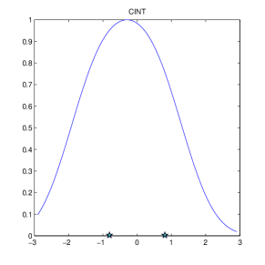
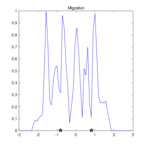
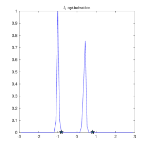
Fig. 2: Results in one realization of the random medium. The abscissa is the cross-range in units $\lambda_{o}L/X$, and the source locations are shown with the stars. We display the CINT and migration images in the top row, and the $l_{1}$ and direct $l_{1}$ optimization results in the bottom row.

We begin with the results in Figure 2, for two sources that are at about $2\lambda_{o}L/X$ apart. The exact source locations are indicated on the abscissa in the plots, where the units are in $\lambda_{o}L/X$. We display in the top row the CINT and migration images, and in the bottom row the solutions of the $l_{1}$ optimization and the direct $l_{1}$ optimization. Both migration and direct $l_{1}$ optimization give spurious peaks, due to the random medium. To confirm this, we show in Figure 3 the results of the direct $l_{1}$ optimization for the same sources in the homogeneous medium, where the reconstruction is very good. The CINT image shown in the top left plot is blurry, and it cannot distinguish the two sources. The $l_{1}$ optimization improves the result, although there is a small shift in the estimate of the source locations. This shift changes from one realization to another, and it is due to the small random fluctuations of the CINT image.

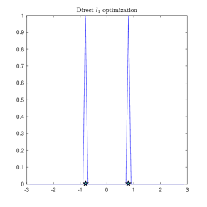
Fig. 3: Result of direct $l_{1}$ optimization in the homogeneous medium. The abscissa is the cross-range in units $\lambda_{o}L/X$, and the source locations are shown with the stars.

To illustrate the robustness of the methods to different realizations of the random medium, we display in Figure 4 the histograms of the number of peaks found by each method at a given cross-range location. We define filtered peaks as local maxima whose values are above $33\%$ of the maximum of the image. The height of the histograms varies among the plots in Figure 4 because each method finds a different number of peaks. On the average, the migration images have $9.5$ peaks, the direct $l_{1}$ method finds $9.65$ peaks, the CINT image has $1.01$ peaks and the $l_{1}$ optimization finds $2.04$ peaks. While both migration and direct $l_{1}$ find many spurious peaks, that are far from the source locations, the $l_{1}$ optimization separates well the two sources and almost always peaks at their true locations.

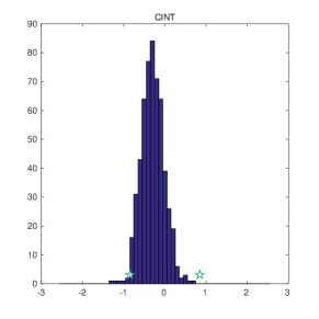
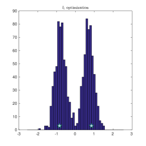
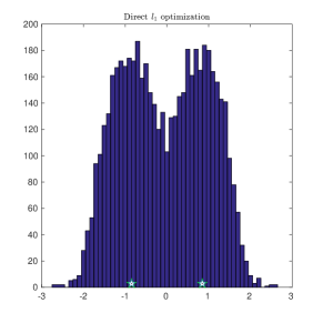
Fig. 4: Histogram of the number of peaks obtained in $500$ realizations of the random medium. The abscissa is the cross-range in units $\lambda_{o}L/X$, and the source locations are shown with the stars. We display the results for the CINT and migration images in the top row, and the $l_{1}$ and direct $l_{1}$ optimization results in the bottom row. The heights of the histograms are different because each method finds a different number of peaks. On the average, the number of peaks found in simulations are   Migration: 9.5,    CINT: 1.01,    $l_{1}$ optimization: 2.04,    Direct $l_{1}$ optimization: 9.65.

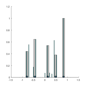
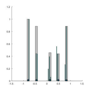
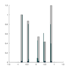
Fig. 5: We display $l_{1}$ optimization results in one realization of the random medium, for $5$ sources with locations indicated by the stars in the abscissa. The units of the abscissa are in $\lambda_{o}L/X$. The dark thin bars show the reconstruction and the light gray bars give the aggregated values of the reconstruction in the intervals of length $r=L\lambda_{o}/(4X)$, centered at the source locations. The mesh size is, clockwise, starting from the top left, $H=1,1/2,1/8$ and $1/4$ of $\lambda_{o}L/X$. The results improve as we refine the mesh.

We display in Figure 5 the effect of the mesh size $H$ on the $l_{1}$ optimization results. Because we have $5$ sources in this simulation, that are closer apart than $\lambda_{o}L/X$, we do not expect a nearly exact reconstruction with the $l_{1}$ optimization. Thus, we display in addition to the actual reconstructions the aggregated values recovered in the intervals of length $r=\lambda_{o}L/(4X),$ centered at the true source locations. We observe that the results improve as we decrease the mesh size from $H=\lambda_{o}L/X$ to $\lambda_{o}L/(8X)$. This is due to the fact that the sources are off the grid, and the discretization error decreases as we reduce $H$.

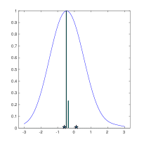
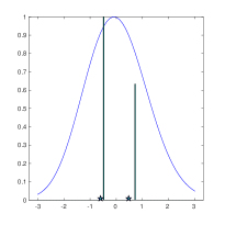
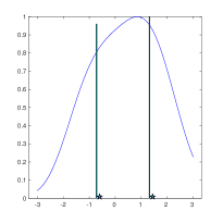
Fig. 6: We display $l_{1}$ optimization results in one realization of the random medium, for $2$ sources separated by, from left to right, $3/4$, $1$ and $2$ $\lambda_{o}L/X$. The units of the abscissa are in $\lambda_{o}L/X$.

The last illustration, in Figure 6, shows the effect of the source separation on the quality of the reconstructions. As expected from the results in section 5, the reconstruction is better when the sources are further apart.

7 Summary

We studied receiver array imaging of remote localized sources in random media, using convex optimization. The scattering regime is defined by precise scaling assumptions, and leads to large random wavefront distortions of the waves measured at the array. Conventional imaging methods like reverse time migration, also known as backprojection [4, 20], or standard $l_{1}$ optimization [14, 19], cannot deal with such distortions and produce poor and unreliable results. We base our imaging on the coherent interferometric (CINT) method [9] which mitigates random media effects like wavefront distortions at the expense of image resolution. The goal of the convex optimization is to remove the blur in the CINT images and thus improve the source localization. We show with a detailed analysis that under generic conditions the CINT imaging function is approximately a convolution of a blurring kernel with the discretized unknown source intensity on the imaging mesh. The kernel has a generic expression, that depends on the known CINT resolution limits obtained in [9, 10, 6] for various wave propagation models. The optimization seeks to undo this convolution. The analysis and numerical simulations show that it gives very good estimates of the source locations when they are sufficiently far apart. This is in agreement with the results in [11]. We also show that when the sources are clustered together, the estimates are not close to the true locations pointwise, but they are supported in their vicinity.

Appendix A The paraxial approximation

Equation (30) follows easily from the Taylor expansion

$$|\vec{\bm{x}}-\vec{\bm{y}}|=\sqrt{y_{3}^{2}+|\bm{x}-\bm{y}|^{2}}=L\left[1+O\left(\frac{D_{3}}{L}\right)+O\left(\frac{a^{2}}{L^{2}}\right)\right],$$

where we used that $y_{3}=L+O(D_{3})$, $|\bm{x}|=O(a)$ and $|\bm{y}|=O(D)\leq O(a)$. For the phase we obtain similarly

$$k_{o}|\vec{\bm{x}}-\vec{\bm{y}}|=k_{o}\sqrt{y_{3}^{2}+|\bm{y}-\bm{x}|^{2}}=k_{o}\left(y_{3}+\frac{|\bm{x}-\bm{y}|^{2}}{2y_{3}}\right)+O\left(\frac{k_{o}|\bm{x}-\bm{y}|^{4}}{y_{3}^{3}}\right),$$

where $k_{o}=\omega_{o}/c_{o}=2\pi/\lambda_{o}$. Expanding the square in the right hand side and using that $y_{3}=L+O(D_{3})$,

$$k_{o}|\vec{\bm{x}}-\vec{\bm{y}}|=k_{o}\left(y_{3}+\frac{|\bm{x}|^{2}-2\bm{x}\cdot\bm{y}+|\bm{y}|^{2}}{2L}\right)+O\left(\frac{a^{4}}{\lambda_{o}L^{3}}\right)+O\left(\frac{a^{2}D_{3}}{\lambda_{o}L^{2}}\right)+O\left(\frac{aDD_{3}}{\lambda_{o}L^{2}}\right)+O\left(\frac{D^{2}D_{3}}{\lambda_{o}L^{2}}\right).$$

The last two terms in the remainder are dominated by the previous ones, because $D<a$, and approximation (29) follows.

Appendix B Derivation of the statistical moments

We begin with the second moments of the Gaussian process (22), with Gaussian autocorrelation (17), and then prove Propositions 1 and 2.

Consider points $\vec{\bm{y}}$ and $\vec{\bm{y}}^{\prime}$ in the imaging region, so that $|\vec{\bm{x}}-\vec{\bm{y}}|\geq|\vec{\bm{x}}^{\prime}-\vec{\bm{y}}^{\prime}|$, and write

$$\mathbb{E}\left[\nu(\vec{\bm{x}},\vec{\bm{y}})\nu(\vec{\bm{x}}^{\prime},\vec{\bm{y}}^{\prime})\right] =\frac{\sqrt{|\vec{\bm{x}}^{\prime}-\vec{\bm{y}}^{\prime}||\vec{\bm{x}}-\vec{\bm{y}}|}}{\sqrt{2\pi}\ell}\iint_{0}^{1}d\vartheta d\vartheta^{\prime}\,e^{-\frac{1}{2\ell^{2}}\left|(\vartheta^{\prime}-\vartheta)(\vec{\bm{x}}-\vec{\bm{y}})+\vartheta^{\prime}(\vec{\bm{x}}^{\prime}-\vec{\bm{x}})+(1-\vartheta^{\prime})(\vec{\bm{y}}^{\prime}-\vec{\bm{y}})\right|^{2}}$$

$$=\sqrt{\frac{|\vec{\bm{x}}^{\prime}-\vec{\bm{y}}^{\prime}|}{|\vec{\bm{x}}-\vec{\bm{y}}|}}\int_{0}^{1}d\vartheta^{\prime}\int_{-(1-\vartheta^{\prime})|\vec{\bm{x}}-\vec{\bm{y}}|/\ell}^{\vartheta^{\prime}|\vec{\bm{x}}-\vec{\bm{y}}|/\ell}\frac{d\widetilde{\vartheta}}{\sqrt{2\pi}}\,e^{-\frac{1}{2}\left|\widetilde{\vartheta}\frac{(\vec{\bm{x}}-\vec{\bm{y}})}{|\vec{\bm{x}}-\vec{\bm{y}}|}+\vartheta^{\prime}\frac{(\vec{\bm{x}}^{\prime}-\vec{\bm{x}})}{\ell}+(1-\vartheta^{\prime})\frac{(\vec{\bm{y}}^{\prime}-\vec{\bm{y}})}{\ell}\right|^{2}},$$

where we changed variables

$$(\vartheta,\vartheta^{\prime})\leadsto(\widetilde{\vartheta},\vartheta^{\prime}),~{}~{}\widetilde{\vartheta}=(\vartheta^{\prime}-\vartheta)|\vec{\bm{x}}-\vec{\bm{y}}|/\ell.$$

Let $\vec{\bm{m}}=(\vec{\bm{x}}-\vec{\bm{y}})/|\vec{\bm{x}}-\vec{\bm{y}}|$ and note that since $|\vec{\bm{x}}-\vec{\bm{y}}|\sim L\gg\ell$ and the Gaussian is negligible for $|\widetilde{\vartheta}|>3$, we can extend the $\widetilde{\vartheta}$ integral to the real line and obtain

$$\mathbb{E}\left[\nu(\vec{\bm{x}},\vec{\bm{y}})\nu(\vec{\bm{x}}^{\prime},\vec{\bm{y}}^{\prime})\right]\approx\sqrt{\frac{|\vec{\bm{x}}^{\prime}-\vec{\bm{y}}^{\prime}|}{|\vec{\bm{x}}-\vec{\bm{y}}|}}\int_{0}^{1}d\vartheta\,e^{-\frac{1}{2\ell^{2}}\left|(I-\vec{\bm{m}}\vec{\bm{m}}^{T})\left[\vartheta(\vec{\bm{x}}^{\prime}-\vec{\bm{x}})+(1-\vartheta)(\vec{\bm{y}}^{\prime}-\vec{\bm{y}})\right]\right|^{2}}.$$ (104)

In the system of coordinates centered at the array, we calculate

$$\vec{\bm{m}}=\frac{(\bm{x},0)-(\bm{y},L+y_{3})}{\sqrt{(L+y_{3})^{2}+|\bm{x}-\bm{y}|^{2}}}=\left[-\vec{\bm{e}}_{3}+\frac{(\bm{x}-\bm{y},0)}{L+y_{3}}\right]\left[1+O\left(\frac{a^{2}}{L^{2}}\right)\right],$$

with $\vec{\bm{e}}_{3}$ the unit vector in the range direction, and obtain

$$|\vec{\bm{m}}+\vec{\bm{e}}_{3}|=O\left(\frac{a}{L}\right)\ll 1.$$

The projections on the plane orthogonal to $\vec{\bm{m}}$ are

$$(I-\vec{\bm{m}}\vec{\bm{m}}^{T})\frac{(\vec{\bm{x}}^{\prime}-\vec{\bm{x}})}{\ell} =\frac{(\bm{x}^{\prime}-\bm{x},0)}{\ell}+O\left(\frac{a^{2}}{\ell L}\right),$$ (105)

$$(I-\vec{\bm{m}}\vec{\bm{m}}^{T})\frac{(\vec{\bm{y}}^{\prime}-\vec{\bm{y}})}{\ell} =\frac{(\bm{y}^{\prime}-\bm{y},0)}{\ell}+O\left(\frac{aD}{\ell L}\right)+O\left(\frac{aD_{3}}{\ell L}\right),$$ (106)

with negligible residuals by assumptions (39)-(40) and (43), which give

$$\frac{a^{2}}{\ell L}\ll\frac{\sqrt{\lambda_{o}L}}{\ell}\ll 1,\qquad\frac{aD_{3}}{\ell L}\ll\frac{\lambda_{o}L}{\ell a}<\frac{\lambda_{o}L}{\ell^{2}}\ll 1.$$

Thus, we can approximate (104) as

$$\mathbb{E}\left[\nu(\vec{\bm{x}},\vec{\bm{y}})\nu(\vec{\bm{x}}^{\prime},\vec{\bm{y}}^{\prime})\right]\approx\sqrt{\frac{|\vec{\bm{x}}^{\prime}-\vec{\bm{y}}^{\prime}|}{|\vec{\bm{x}}-\vec{\bm{y}}|}}\int_{0}^{1}d\vartheta\,e^{-\frac{1}{2\ell^{2}}\left|\vartheta(\bm{x}^{\prime}-\bm{x})+(1-\vartheta)(\bm{y}^{\prime}-\bm{y})\right|^{2}}.$$ (107)

This expression can be simplified further for small offsets satisfying $|\bm{y}^{\prime}-\bm{y}|\ll\ell$ and $|\bm{x}^{\prime}-\bm{x}|\ll\ell$, by expanding the exponential and then integrating in $\vartheta$,

$$\mathbb{E}\left[\nu(\vec{\bm{x}},\vec{\bm{y}})\nu(\vec{\bm{x}}^{\prime},\vec{\bm{y}}^{\prime})\right]\approx\sqrt{\frac{|\vec{\bm{x}}^{\prime}-\vec{\bm{y}}^{\prime}|}{|\vec{\bm{x}}-\vec{\bm{y}}|}}\left[1-\frac{|\bm{y}^{\prime}-\bm{y}|^{2}+(\bm{y}^{\prime}-\bm{y})\cdot(\bm{x}^{\prime}-\bm{x})+|\bm{x}^{\prime}-\bm{x}|^{2}}{6\ell^{2}}\right].$$ (108)

Note that the small receiver offset condition is consistent with $|\bm{x}^{\prime}-\bm{x}|\ll X\sim X_{d}\ll\ell$ used in the CINT image formation.

The proof of Proposition 1 follows easily from (108) and definitions (20), (22). Because the process $\nu(\vec{\bm{x}},\vec{\bm{y}})$ is Gaussian, we have

$$\mathbb{E}\left[\widehat{G}(\vec{\bm{x}},\vec{\bm{y}},\omega)\right] \approx\widehat{G}_{o}(\vec{\bm{x}},\vec{\bm{y}},\omega)\mathbb{E}\left[\exp\left(i\frac{(2\pi)^{1/4}}{2}k\sigma\sqrt{\ell|\vec{\bm{x}}-\vec{\bm{y}}|}\nu(\vec{\bm{x}},\vec{\bm{y}})\right)\right]$$

$$\approx\widehat{G}_{o}(\vec{\bm{x}},\vec{\bm{y}},\omega)\exp\left\{-\frac{\sqrt{2\pi}}{8}k^{2}\sigma^{2}\ell|\vec{\bm{x}}-\vec{\bm{y}}|\mathbb{E}\left[\nu^{2}(\vec{\bm{x}},\vec{\bm{y}})\right]\right\}$$

$$=\widehat{G}_{o}(\vec{\bm{x}},\vec{\bm{y}},\omega)\exp\left[-\frac{\sqrt{2\pi}}{8}k^{2}\sigma^{2}\ell|\vec{\bm{x}}-\vec{\bm{y}}|\right].$$ (109)

This is equation (32) with scattering mean free path $\mathcal{S}(\omega)$ defined as in (33). $\Box$

To prove Proposition 2 we use again definitions (20) and (22), the Gaussianity of the process $\nu$, and result (104) to write

$$\mathbb{E}\left[\widehat{G}(\vec{\bm{x}},\vec{\bm{y}},\omega+\widetilde{\omega}/2)\overline{\widehat{G}(\vec{\bm{x}}^{\prime},\vec{\bm{y}}^{\prime},\omega-\widetilde{\omega}/2)}\right]\approx\widehat{G}_{o}(\vec{\bm{x}},\vec{\bm{y}},\omega+\widetilde{\omega}/2)\overline{\widehat{G}_{o}(\vec{\bm{x}}^{\prime},\vec{\bm{y}}^{\prime},\omega-\widetilde{\omega}/2)}\,\mathcal{E},$$ (110)

with

$$\mathcal{E}=\exp \left\{-\frac{\sqrt{2\pi}}{8}\left(\frac{\omega+\widetilde{\omega}/2}{c_{o}}\right)^{2}\sigma^{2}\ell|\vec{\bm{x}}-\vec{\bm{y}}|-\frac{\sqrt{2\pi}}{8}\left(\frac{\omega-\widetilde{\omega}/2}{c_{o}}\right)^{2}\sigma^{2}\ell|\vec{\bm{x}}^{\prime}-\vec{\bm{y}}^{\prime}|\right.$$

$$\left.+\frac{\sqrt{2\pi}(\omega^{2}-\widetilde{\omega}^{2}/4)}{4c_{o}^{2}}\sigma^{2}\ell|\vec{\bm{x}}^{\prime}-\vec{\bm{y}}^{\prime}|\int_{0}^{1}d\vartheta\,e^{-\frac{1}{2\ell^{2}}\left|\vartheta(\bm{x}^{\prime}-\bm{x})+(1-\vartheta)(\bm{y}^{\prime}-\bm{y})\right|^{2}}\right\}.$$ (111)

Note that

$$\frac{\sqrt{2\pi}}{8}\left(\frac{\omega+\widetilde{\omega}/2}{c_{o}}\right)^{2}\sigma^{2}\ell|\vec{\bm{x}}-\vec{\bm{y}}| =\frac{|\vec{\bm{x}}-\vec{\bm{y}}|}{\mathcal{S}(\omega+\widetilde{\omega}/2)}\gg 1,$$

$$\frac{\sqrt{2\pi}}{8}\left(\frac{\omega-\widetilde{\omega}/2}{c_{o}}\right)^{2}\sigma^{2}\ell|\vec{\bm{x}}^{\prime}-\vec{\bm{y}}^{\prime}| =\frac{|\vec{\bm{x}}^{\prime}-\vec{\bm{y}}^{\prime}|}{\mathcal{S}(\omega-\widetilde{\omega}/2)}\gg 1,$$

so $\mathcal{E}$ is exponentially small unless the last term in (111) compensates the first two. This happens only when $|\bm{y}-\bm{y}^{\prime}|\ll\ell$. For other offsets the integral over $\vartheta$ is small and, consequently, $\mathcal{E}\approx 0.$

When $|\bm{y}-\bm{y}^{\prime}|\ll\ell$, we can approximate the $\vartheta$ integral as in (108), and obtain

$$\mathcal{E}\approx\exp \left\{-\frac{\sqrt{2\pi}}{8}\left(\frac{\omega+\widetilde{\omega}/2}{c_{o}}\right)^{2}\sigma^{2}\ell|\vec{\bm{x}}-\vec{\bm{y}}|-\frac{\sqrt{2\pi}}{8}\left(\frac{\omega-\widetilde{\omega}/2}{c_{o}}\right)^{2}\sigma^{2}\ell|\vec{\bm{x}}^{\prime}-\vec{\bm{y}}^{\prime}|\right.$$

$$\left.+\frac{\sqrt{2\pi}(\omega^{2}-\widetilde{\omega}^{2}/4)}{4c_{o}^{2}}\sigma^{2}\ell|\vec{\bm{x}}^{\prime}-\vec{\bm{y}}^{\prime}|\left[1-\frac{|\bm{y}^{\prime}-\bm{y}|^{2}+(\bm{y}^{\prime}-\bm{y})\cdot(\bm{x}^{\prime}-\bm{x})+|\bm{x}^{\prime}-\bm{x}|^{2}}{6\ell^{2}}\right]\right\}.$$ (112)

Rearranging the terms and using definition (33) of the scattering mean free path we get

$$\mathcal{E}\approx\exp \left\{-\frac{|\vec{\bm{x}}-\vec{\bm{y}}|-|\vec{\bm{x}}^{\prime}-\vec{\bm{y}}^{\prime}|}{\mathcal{S}(\omega)}-\frac{\sqrt{2\pi}\sigma^{2}\ell\widetilde{\omega}^{2}}{8c_{o}^{2}}\left(\frac{|\vec{\bm{x}}-\vec{\bm{y}}|+3|\vec{\bm{x}}^{\prime}-\vec{\bm{y}}^{\prime}|}{4}\right)-\frac{\sqrt{2\pi}\sigma^{2}\ell\omega\widetilde{\omega}}{8c_{o}^{2}}(|\vec{\bm{x}}-\vec{\bm{y}}|-|\vec{\bm{x}}^{\prime}-\vec{\bm{y}}^{\prime}|)\right.$$

$$\left.-\frac{\sqrt{2\pi}(\omega^{2}-\widetilde{\omega}^{2}/4)\sigma^{2}|\vec{\bm{x}}^{\prime}-\vec{\bm{y}}^{\prime}|}{24c_{o}^{2}\ell}\left(|\bm{y}^{\prime}-\bm{y}|^{2}+(\bm{y}^{\prime}-\bm{y})\cdot(\bm{x}^{\prime}-\bm{x})+|\bm{x}^{\prime}-\bm{x}|^{2}\right)\right\}.$$ (113)

Recall that $|\vec{\bm{x}}-\vec{\bm{y}}|\geq|\vec{\bm{x}}^{\prime}-\vec{\bm{y}}^{\prime}|$, and conclude from the decay of the first term that $\mathcal{E}$ is large if

$$|\vec{\bm{x}}-\vec{\bm{y}}|-|\vec{\bm{x}}^{\prime}-\vec{\bm{y}}|=O(\mathcal{S}(\omega)).$$

Substituting in (113), and using the scales

$$\Omega_{d}=\frac{2c_{o}}{(2\pi)^{1/4}\sigma\sqrt{\ell|\vec{\bm{x}}-\vec{\bm{y}}|}},\quad X(\omega)=\frac{\sqrt{3}\ell\Omega_{d}}{\omega},$$ (114)

we get

$$\mathcal{E}\approx\exp \left\{-\frac{|\vec{\bm{x}}-\vec{\bm{y}}|-|\vec{\bm{x}}^{\prime}-\vec{\bm{y}}^{\prime}|}{\mathcal{S}(\omega)}-\frac{\widetilde{\omega}^{2}}{2\Omega_{d}^{2}}\left[1+O\left(\frac{\mathcal{S}(\omega)}{L}\right)\right]+O\left(\frac{\sigma^{2}\ell\omega\widetilde{\omega}\mathcal{S}(\omega)}{c_{o}^{2}}\right)\right.$$

$$\left.-\frac{(|\bm{y}^{\prime}-\bm{y}|^{2}+(\bm{y}^{\prime}-\bm{y})\cdot(\bm{x}^{\prime}-\bm{x})+|\bm{x}^{\prime}-\bm{x}|^{2})}{2X(\omega)^{2}}\left[1+O\left(\frac{\mathcal{S}(\omega)}{L}\right)+O\left(\frac{\Omega_{d}^{2}}{\omega^{2}}\right)\right]\right\}.$$ (115)

This equation simplifies because $\mathcal{S}(\omega)\ll L$ and $\Omega_{d}\ll\omega=O(\omega_{o})$. Moreover, (115) is large only when $|\widetilde{\omega}|\lesssim\Omega_{d}$, so we estimate using definitions (33) and (114) and the assumption (41) that

$$\frac{\sigma^{2}\ell\omega\widetilde{\omega}\mathcal{S}}{c_{o}^{2}}\lesssim O\left(\frac{\sigma^{2}\ell\omega_{o}\Omega_{d}\mathcal{S}}{c_{o}^{2}}\right)=O\left(\frac{\lambda_{o}}{\sigma\sqrt{\ell L}}\right)\ll 1.$$

Similarly, $\mathcal{E}$ is large for cross-range offsets of at most $O(X)$, so we can write

$$|\vec{\bm{x}}-\vec{\bm{y}}|-|\vec{\bm{x}}^{\prime}-\vec{\bm{y}}^{\prime}|\approx y_{3}-y_{3}^{\prime}+\frac{|\bm{x}|^{2}-|\bm{x}^{\prime}|^{2}}{2L}+\frac{|\bm{y}|^{2}-|\bm{y}^{\prime}|^{2}}{2L}-\frac{\bm{x}\cdot\bm{y}-\bm{x}^{\prime}\cdot\bm{y}^{\prime}}{L}=y_{3}-y_{3}^{\prime}+O\left(\frac{aX}{L}\right).$$

We also have $X\sim X_{d}$, and

$$\frac{aX_{d}}{\mathcal{S}L}=O\left(\frac{aX_{d}}{L}\frac{\sigma^{2}\ell}{\lambda_{o}^{2}}\right)=O\left(\frac{a\sigma\ell^{3/2}}{\lambda_{o}L^{3/2}}\right)\ll O\left[\frac{\sigma\ell^{3/2}}{(\lambda_{o}L)^{3/4}}\right]\ll O\left(\frac{\ell^{2}}{\lambda_{o}^{1/4}L^{1+3/4}}\right)\ll O\left[\left(\frac{\lambda_{o}}{L}\right)^{1/4}\right]\ll 1,$$

where the two equalities are by definition (33) and (35) of $\mathcal{S}$ and $X_{d}$, the first inequality is by (39), the second by (41), the third by (40), and the last by (18). Gathering the results we arrive at the approximation

$$\mathcal{E}\approx\exp \left[-\frac{|y_{3}-y_{3}^{\prime}|}{\mathcal{S}(\omega)}-\frac{\widetilde{\omega}^{2}}{2\Omega_{d}^{2}}-\frac{|\bm{y}^{\prime}-\bm{y}|^{2}+(\bm{y}^{\prime}-\bm{y})\cdot(\bm{x}^{\prime}-\bm{x})+|\bm{x}^{\prime}-\bm{x}|^{2}}{2X^{2}(\omega)}\right].$$ (116)

The statement of Proposition 2 follows from this equation and $|\omega-\omega_{o}|\lesssim\pi B\ll\omega_{o}$. $\Box$

Appendix C Consistency of scaling

The scaling (41) is consistent because

$$\frac{(\ell/L)^{3/2}}{\sqrt{\ell\lambda_{o}}/L}=\frac{\ell}{\sqrt{\lambda_{o}L}}\gg 1\quad\mbox{and}\quad\frac{\sqrt{\ell\lambda_{o}}/{L}}{\lambda_{o}/\sqrt{\ell L}}=\frac{\ell}{\sqrt{\lambda_{o}L}}\gg 1,$$

where we used (40).

The scaling (44) is consistent because by assumption (39) and (35),

$$\frac{(a/L)^{2}}{\lambda_{o}L/(aX_{d})}=\frac{a^{4}}{\lambda_{o}L^{3}}\frac{X_{d}}{a}\ll\frac{\ell}{a}<1.$$

We also have

$$\frac{\lambda_{o}L/(aX_{d})}{\Omega_{d}/\omega_{o}}=O\left(\frac{\lambda_{0}L}{a\ell(\Omega_{d}/\omega_{o})^{2}}\right)=O\left(\frac{\sigma^{2}L^{2}}{a\lambda_{o}}\right)\ll\frac{\ell}{a}<1,$$

so (44) implies $B\ll\Omega_{d}.$

Definition (35) and assumptions (40), (41) give

$$\frac{\lambda_{o}L}{X_{d}}=O\left(\frac{\lambda_{o}L}{\ell}\frac{\omega_{o}}{\Omega_{d}}\right)=O\left(\sigma\frac{L^{3/2}}{\ell^{1/2}}\right)\ll\sqrt{\lambda_{o}L}\ll\ell.$$

This verifies that the assumptions (43) on $D$ are consistent.

The assumptions (43) on $D_{3}$ are consistent in the narrowband regime, when (44) holds, because by (42) we have $\Omega/B=O(1)$ and

$$\frac{c_{o}/B}{\lambda_{o}L^{2}/a^{2}}=O\left(\frac{\omega_{o}}{B}\frac{a^{2}}{L^{2}}\right)\ll 1.$$

In the broadband regime $\Omega=\Omega_{d}$ and assumptions (43) on $D_{3}$ are consistent because

$$\frac{c_{o}/\Omega_{d}}{\lambda_{o}L^{2}/a^{2}}=O\left(\frac{\sigma\sqrt{\ell L}}{\lambda_{o}L^{2}/a^{2}}\right)\ll\frac{\ell}{L}\ll 1,$$

by definition (35) and assumptions (39) and (41). Moreover, assumption (47) is consistent because

$$\frac{\lambda_{o}^{2/3}\ell^{1/6}/L^{5/6}}{\lambda_{o}/\sqrt{\ell L}}=\left(\frac{\ell}{\sqrt{\lambda_{o}L}}\right)^{2/3}\gg 1,\qquad\frac{\lambda_{o}^{2/3}\ell^{1/6}/L^{5/6}}{\sqrt{\lambda_{o}\ell}/L}=\left(\frac{\sqrt{\lambda_{o}L}}{\ell}\right)^{1/3}\ll 1,$$

by assumption (40).

Appendix D Derivation of the CINT kernel

We begin with the expression (11) of the CINT kernel, and use the Gaussian pulse, thresholding windows and apodization to obtain

$$\kappa(\vec{\bm{y}},\vec{\bm{z}},\vec{\bm{z}}^{\prime})\approx \frac{N_{r}^{2}\sqrt{2\pi}}{a^{4}B}\int d\bm{x}\,e^{-\frac{|\bm{x}|^{2}}{(a/6)^{2}}}\int d\widetilde{\bm{x}}\,e^{-\frac{|\widetilde{\bm{x}}|^{2}}{2X^{2}}-\frac{|\widetilde{\bm{x}}|^{2}}{4(a/6)^{2}}}\int d\omega\,e^{-\frac{(\omega-\omega_{o})^{2}}{2B^{2}}}\int d\widetilde{\omega}\,e^{-\frac{\widetilde{\omega}^{2}}{2\Omega^{2}}-\frac{\widetilde{\omega}^{2}}{8B^{2}}}$$

$$\times\widehat{G}\left(\left(\bm{x}+\widetilde{\bm{x}}/2,0\right),\vec{\bm{z}},\omega+\widetilde{\omega}/2\right)\overline{\widehat{G}\left(\left(\bm{x}-\widetilde{\bm{x}}/2,0\right),\vec{\bm{z}}^{\prime},\omega-\widetilde{\omega}/2\right)}$$

$$\times\exp\left[-i\frac{(\omega+\widetilde{\omega}/2)}{c_{o}}\left|(\bm{x}+\widetilde{\bm{x}}/2,0)-\vec{\bm{y}}\right|+i\frac{(\omega-\widetilde{\omega}/2)}{c_{o}}\left|(\bm{x}-\widetilde{\bm{x}}/2,0)-\vec{\bm{y}}\right|\right],$$ (117)

for points $\vec{\bm{y}}=(\bm{y},y_{3})$, $\vec{\bm{z}}=(\bm{z},z_{3})$ and $\vec{\bm{z}}^{\prime}=(\bm{z}^{\prime},z_{3}^{\prime})$ in the imaging region. The integration over $\bm{x}$ and $\widetilde{\bm{x}}$ extends to the whole plane $\mathbb{R}^{2}$, and those over $\omega$ and $\widetilde{\omega}$ to the real line, with the aperture and bandwidth restrictions ensured by the Gaussians. Because CINT is statistically stable in our scaling, we may approximate the right hand side of (118) by its expectation. Using (38) and the paraxial approximation (31), we obtain

$$\kappa(\vec{\bm{y}},\vec{\bm{z}},\vec{\bm{z}}^{\prime})\approx \frac{N_{r}^{2}\sqrt{2\pi}}{a^{4}B(4\pi L)^{2}}e^{-\frac{|\bm{z}-\bm{z}^{\prime}|^{2}}{2X_{d}^{2}}}\int d\bm{x}\,e^{-\frac{|\bm{x}|^{2}}{(a/6)^{2}}}\int d\widetilde{\bm{x}}\,e^{-\frac{|\widetilde{\bm{x}}|^{2}}{2X_{e}^{2}}-\frac{\widetilde{\bm{x}}\cdot(\bm{z}-\bm{z}^{\prime})}{2X_{d}^{2}}}\int d\omega\,e^{-\frac{(\omega-\omega_{o})^{2}}{2B^{2}}}\int d\widetilde{\omega}\,e^{-\frac{\widetilde{\omega}^{2}}{2\Omega_{e}^{2}}}$$

$$\times\exp\left\{i\frac{\widetilde{\omega}}{c_{o}}\left[\frac{z_{3}+z_{3}^{\prime}}{2}-y_{3}+\frac{1}{2L}\left(\frac{|\bm{z}|^{2}+|\bm{z}^{\prime}|^{2}}{2}-|\bm{y}|^{2}\right)-\frac{\bm{x}}{L}\cdot\left(\frac{\bm{z}+\bm{z}^{\prime}}{2}-\bm{y}\right)-\frac{\widetilde{\bm{x}}}{4L}\cdot(\bm{z}-\bm{z}^{\prime})\right]\right\}$$

$$\times\exp\left\{i\frac{\omega}{c_{o}}\left[z_{3}-z_{3}^{\prime}+\frac{|\bm{z}|^{2}-|\bm{z}^{\prime}|^{2}}{2L}-\frac{\bm{x}\cdot(\bm{z}-\bm{z}^{\prime})}{L}-\frac{\widetilde{\bm{x}}}{L}\cdot\left(\frac{\bm{z}+\bm{z}^{\prime}}{2}-\bm{y}\right)\right]\right\},$$ (118)

with $X_{e}=O(X_{d})$ and $\Omega_{e}=O(B)$ defined in (53). Note that the last term in the second line of (118) is negligible, because by assumptions (39), (44) and definition (35),

$$\frac{\widetilde{\omega}\widetilde{\bm{x}}\cdot(\bm{z}-\bm{z}^{\prime})}{4Lc_{o}}=O\left(\frac{BX_{d}^{2}}{c_{o}L}\right)=O\left(\frac{B}{\omega_{o}}\frac{aX_{d}}{\lambda_{o}L}\frac{X_{d}}{a}\right)\ll 1,$$

in the narrowband case. Moreover, in the broadband case

$$\frac{\widetilde{\omega}\widetilde{\bm{x}}\cdot(\bm{z}-\bm{z}^{\prime})}{4Lc_{o}}=O\left(\frac{\Omega_{d}X_{d}^{2}}{c_{o}L}\right)=O\left(\frac{\ell^{2}}{\lambda_{o}L}\frac{\Omega_{d}^{3}}{\omega_{o}^{3}}\right)=O\left(\frac{\lambda_{o}^{2}\ell^{1/2}}{\sigma^{3}L^{5/2}}\right)\ll 1,$$

where the first equalities are by definitions (35), and the bound is by (47). Let us introduce the center and difference coordinates

$$\overline{\bm{z}}=\frac{\bm{z}+\bm{z}^{\prime}}{2},\qquad\widetilde{\bm{z}}=\bm{z}-\bm{z}^{\prime},\qquad\overline{z}_{3}=\frac{z_{3}+z_{3}^{\prime}}{2},\qquad\widetilde{z}_{3}=z_{3}-z_{3}^{\prime},$$ (119)

and note that

$$\frac{\widetilde{\omega}}{c_{o}L}\left(\frac{|\bm{z}|^{2}+|\bm{z}^{\prime}|^{2}}{2}-|\bm{y}|^{2}\right)=\frac{\widetilde{\omega}}{c_{o}}\frac{(|\overline{\bm{z}}|^{2}-|\bm{y}|^{2})}{L}+\frac{\widetilde{\omega}|\widetilde{\bm{z}}|^{2}}{4c_{o}L}\approx\frac{\widetilde{\omega}}{c_{o}}\frac{(|\overline{\bm{z}}|^{2}-|\bm{y}|^{2})}{L},$$

because

$$\frac{\widetilde{\omega}}{c_{o}}\frac{|\widetilde{\bm{x}}|^{2}}{L}=O\left(\frac{\Omega_{d}X_{d}^{2}}{c_{o}L}\right)\ll 1.$$

The kernel (118) simplifies as

$$\kappa(\vec{\bm{y}},\vec{\bm{z}},\vec{\bm{z}}^{\prime})\approx \frac{N_{r}^{2}\sqrt{2\pi}}{a^{4}B(4\pi L)^{2}}e^{-\frac{|\widetilde{\bm{z}}|^{2}}{2X_{d}^{2}}}\int d\widetilde{\omega}\,\exp\left[-\frac{\widetilde{\omega}^{2}}{2\Omega_{e}^{2}}+i\widetilde{\omega}\left(\frac{\overline{z}_{3}-y_{3}}{c_{o}}+\frac{|\overline{\bm{z}}|^{2}-|\bm{y}|^{2}}{2Lc_{o}}\right)\right]$$

$$\times\int d\omega\,\exp\left[-\frac{(\omega-\omega_{o})^{2}}{2B^{2}}+i\omega\left(\frac{\widetilde{z}_{3}}{c_{o}}+\frac{\overline{\bm{z}}\cdot\widetilde{\bm{z}}}{Lc_{o}}\right)\right]$$

$$\times\int d\widetilde{\bm{x}}\,\exp\left[-\frac{|\widetilde{\bm{x}}|^{2}}{2X_{e}^{2}}-\widetilde{\bm{x}}\cdot\left(\frac{\widetilde{\bm{z}}}{2X_{d}^{2}}+\frac{i\omega(\overline{\bm{z}}-\bm{y})}{Lc_{o}}\right)\right]$$

$$\times\int d\bm{x}\,\exp\left[-\frac{|\bm{x}|^{2}}{(a/6)^{2}}-i\bm{x}\cdot\left(\frac{\widetilde{\omega}(\overline{\bm{z}}-\bm{y})}{Lc_{o}}+\frac{\omega\widetilde{\bm{z}}}{Lc_{o}}\right)\right],$$ (120)

with $\Omega_{e}$ and $X_{e}$ defined in (53), and after evaluating the last two integrals, we get

$$\kappa(\vec{\bm{y}},\vec{\bm{z}},\vec{\bm{z}}^{\prime})\approx \frac{N_{r}^{2}\sqrt{2\pi}X_{e}^{2}}{288Ba^{2}L^{2}}e^{-\frac{|\widetilde{\bm{z}}|^{2}}{2X_{d}^{2}}}\int d\widetilde{\omega}\,\exp\left[-\frac{\widetilde{\omega}^{2}}{2\Omega_{e}^{2}}+i\widetilde{\omega}\left(\frac{\overline{z}_{3}-y_{3}}{c_{o}}+\frac{|\overline{\bm{z}}|^{2}-|\bm{y}|^{2}}{2Lc_{o}}\right)\right]$$

$$\times\int d\omega\,\exp\left[-\frac{(\omega-\omega_{o})^{2}}{2B^{2}}+i\omega\left(\frac{\widetilde{z}_{3}}{c_{o}}+\frac{\overline{\bm{z}}\cdot\widetilde{\bm{z}}}{Lc_{o}}\right)\right]$$

$$\times\exp\left[-\frac{X_{e}^{2}}{2}\left|\frac{\omega(\overline{\bm{z}}-\bm{y})}{Lc_{o}}-\frac{i\widetilde{\bm{z}}}{2X_{d}^{2}}\right|^{2}-\frac{1}{2}\left(\frac{a}{6\sqrt{2}}\right)^{2}\left|\frac{\widetilde{\omega}(\overline{\bm{z}}-\bm{y})}{Lc_{o}}+\frac{\omega\widetilde{\bm{z}}}{Lc_{o}}\right|^{2}\right].$$ (121)

Let us change variables ${\it w}=\omega-\omega_{o}$ and use the notation

$$\overline{\bm{\zeta}}=\frac{\overline{\bm{z}}-\bm{y}}{L/(k_{o}X_{e})},\qquad\widetilde{\bm{\zeta}}=\frac{\widetilde{\bm{z}}}{6\sqrt{2}L/(k_{o}a)},\qquad\beta=\frac{\overline{z}_{3}-y_{3}}{c_{o}/\Omega_{e}}+\frac{|\overline{\bm{z}}|^{2}-|\bm{y}|^{2}}{2Lc_{o}/\Omega_{e}},\qquad\theta=\frac{\omega_{o}X_{e}}{\Omega_{e}(a/6)}.$$ (122)

Define also

$$\frac{1}{\gamma}=1-\frac{X_{e}^{2}}{4X_{d}^{2}}>\frac{3}{4},$$ (123)

with the inequality implied by the definition of $X_{e}$. Substituting in (121) we get

$$\kappa(\vec{\bm{y}},\vec{\bm{z}},\vec{\bm{z}}^{\prime})\approx \frac{N_{r}^{2}\sqrt{2\pi}X_{e}^{2}}{288Ba^{2}L^{2}}\exp\left[-\frac{|\widetilde{\bm{z}}|^{2}}{2\gamma X_{d}^{2}}-\frac{|\overline{\bm{\zeta}}|^{2}}{2}-\frac{|\widetilde{\bm{\zeta}}|^{2}}{2}+ik_{o}\Big{(}\widetilde{z}_{3}+\frac{\widetilde{\bm{z}}\cdot\overline{\bm{z}}}{L}+\frac{X_{e}^{2}\widetilde{\bm{z}}\cdot(\overline{\bm{z}}-\bm{y})}{2X_{d}^{2}L}\Big{)}\right]$$

$$\times\int d{\it w}\exp\left[-\frac{{\it w}^{2}}{2}\Big{(}\frac{1}{B^{2}}+\frac{|\overline{\bm{\zeta}}|^{2}+|\widetilde{\bm{\zeta}}|^{2}}{\omega_{o}^{2}}\Big{)}+\frac{i{\it w}}{c_{o}}\Big{(}\widetilde{z}_{3}+\frac{\overline{\bm{z}}\cdot\widetilde{\bm{z}}}{L}+\frac{X_{e}^{2}\widetilde{\bm{z}}\cdot(\overline{\bm{z}}-\bm{y})}{2X_{d}^{2}L}\Big{)}-\frac{{\it w}(|\overline{\bm{\zeta}}|^{2}+|\widetilde{\bm{\zeta}}|^{2})}{\omega_{o}}\right]$$

$$\times\int d\widetilde{\omega}\,\exp\left[-\frac{\widetilde{\omega}^{2}}{2\Omega_{e}^{2}}\Big{(}1+\frac{|\overline{\bm{\zeta}}|^{2}}{2\theta^{2}}\Big{)}+\frac{i\widetilde{\omega}}{\Omega_{e}}\Big{(}\beta+\frac{i(\omega_{o}+{\it w})\overline{\bm{\zeta}}\cdot\widetilde{\bm{\zeta}}}{\sqrt{2}\omega_{o}\theta}\Big{)}\right],$$ (124)

and integrate next over $\widetilde{\omega}$. We obtain after rearranging the terms that

$$\kappa(\vec{\bm{y}},\vec{\bm{z}},\vec{\bm{z}}^{\prime})\approx \frac{\pi N_{r}^{2}X_{e}^{2}\Omega_{e}}{144Ba^{2}L^{2}\sqrt{1+\frac{|\overline{\bm{\zeta}}|^{2}}{2\theta^{2}}}}\exp\left[-\frac{|\widetilde{\bm{z}}|^{2}}{2\gamma X_{d}^{2}}-\frac{\Delta^{2}}{2}-\frac{\beta^{2}}{2(1+\frac{|\overline{\bm{\zeta}}|^{2}}{2\theta^{2}})}\right]$$

$$\times\exp\left[ik_{o}\Big{(}\widetilde{z}_{3}+\frac{\widetilde{\bm{z}}\cdot\overline{\bm{z}}}{L}+\frac{X_{e}^{2}\widetilde{\bm{z}}\cdot(\overline{\bm{z}}-\bm{y})}{2X_{d}^{2}L}\Big{)}-\frac{i\beta\overline{\bm{\zeta}}\cdot\widetilde{\bm{\zeta}}}{\sqrt{2}\theta(1+\frac{|\overline{\bm{\zeta}}|^{2}}{2\theta^{2}})}\right]$$

$$\times\int d{\it w}\,\exp\left[-\frac{{\it w}^{2}}{2B^{2}}\Big{(}1+\frac{\Delta^{2}B^{2}}{\omega_{o}^{2}}\Big{)}+\frac{i{\it w}\eta}{B}-\frac{{\it w}\Delta^{2}}{\omega_{o}}\right],$$ (125)

with notation

$$\eta =\frac{B}{c_{o}}\left[\widetilde{z}_{3}+\frac{\overline{\bm{z}}\cdot\widetilde{\bm{z}}}{L}+\frac{X_{e}^{2}\widetilde{\bm{z}}\cdot(\overline{\bm{z}}-\bm{y})}{2X_{d}^{2}L}-\frac{\beta c_{o}\overline{\bm{\zeta}}\cdot\widetilde{\bm{\zeta}}}{\sqrt{2}\omega_{o}\theta(1+\frac{|\overline{\bm{\zeta}}|^{2}}{2\theta^{2}})}\right],$$ (126)

$$\Delta^{2} =|\overline{\bm{\zeta}}|^{2}+|\widetilde{\bm{\zeta}}|^{2}-\frac{|\overline{\bm{\zeta}}\cdot\widetilde{\bm{\zeta}}|^{2}}{2\theta^{2}(1+\frac{|\overline{\bm{\zeta}}|^{2}}{2\theta^{2}})}.$$ (127)

Note that (127) is non-negative because

$$|\widetilde{\bm{\zeta}}|^{2}-\frac{|\overline{\bm{\zeta}}\cdot\widetilde{\bm{\zeta}}|^{2}}{2\theta^{2}(1+\frac{|\overline{\bm{\zeta}}|^{2}}{2\theta^{2}})}=\frac{|\widetilde{\bm{\zeta}}|^{2}}{(1+\frac{|\overline{\bm{\zeta}}|^{2}}{2\theta^{2}})}+\frac{(|\overline{\bm{\zeta}}|^{2}|\widetilde{\bm{\zeta}}|^{2}-|\overline{\bm{\zeta}}\cdot\widetilde{\bm{\zeta}}|^{2})}{(1+\frac{|\overline{\bm{\zeta}}|^{2}}{2\theta^{2}})}\geq\frac{|\widetilde{\bm{\zeta}}|^{2}}{(1+\frac{|\overline{\bm{\zeta}}|^{2}}{2\theta^{2}})}.$$

Now we integrate in ${\it w}$ in equation (125), and obtain

$$\kappa(\vec{\bm{y}},\vec{\bm{z}},\vec{\bm{z}}^{\prime})\approx \frac{\sqrt{2}\pi^{3/2}N_{r}^{2}X_{e}^{2}\Omega_{e}}{144a^{2}L^{2}\sqrt{1+\frac{|\overline{\bm{\zeta}}|^{2}}{2\theta^{2}}}\sqrt{1+\frac{\Delta^{2}B^{2}}{\omega_{o}^{2}}}}\exp\left[-\frac{|\widetilde{\bm{z}}|^{2}}{2\gamma X_{d}^{2}}-\frac{\beta^{2}}{2(1+\frac{|\overline{\bm{\zeta}}|^{2}}{2\theta^{2}})}-\frac{\eta^{2}}{2(1+\frac{B^{2}\Delta^{2}}{\omega_{o}^{2}})}-\frac{\Delta^{2}}{2(1+\frac{B^{2}\Delta^{2}}{\omega_{o}^{2}})}\right]$$

$$\times\exp\left[ik_{o}\Big{(}\widetilde{z}_{3}+\frac{\widetilde{\bm{z}}\cdot\overline{\bm{z}}}{L}+\frac{X_{e}^{2}\widetilde{\bm{z}}\cdot(\overline{\bm{z}}-\bm{y})}{2X_{d}^{2}L}\Big{)}-\frac{i\beta\overline{\bm{\zeta}}\cdot\widetilde{\bm{\zeta}}}{\sqrt{2}\theta(1+\frac{|\overline{\bm{\zeta}}|^{2}}{2\theta^{2}})}-\frac{i\eta B\Delta^{2}}{\omega_{o}(1+\frac{B^{2}\Delta^{2}}{\omega_{o}^{2}})}\right].$$ (128)

This expression simplifies, because the exponential decay in $\Delta^{2}$ ensures that the kernel is large only when $\Delta=O(1)$. Since $B/\omega_{o}\ll 1$ by assumption, we see that

$$\frac{B^{2}\Delta^{2}}{\omega_{o}^{2}}\ll 1.$$ (129)

By the same reasoning, the kernel is large when $|\eta|=O(1)$, but then

$$\left|\frac{\eta B\Delta^{2}}{\omega_{o}(1+\frac{B^{2}\Delta^{2}}{\omega_{o}^{2}})}\right|\approx|\eta|\Delta^{2}\frac{B}{\omega_{o}}=O\left(\frac{B}{\omega_{o}}\right)\ll 1.$$ (130)

We also have from $\Delta=O(1)$ and definition (127) that both $|\overline{\bm{\zeta}}|$ and $|\widetilde{\bm{\zeta}}|$ are $O(1)$. Then, using the definition of $\widetilde{\bm{\zeta}}$ in (122), we can estimate

$$\frac{B}{c_{o}}\left|\frac{\overline{\bm{z}}\cdot\widetilde{\bm{z}}}{L}\right|\leq O\left(\frac{B}{c_{o}}\frac{\lambda_{o}L/{a}a}{L}\right)=O\left(\frac{B}{\omega_{o}}\right)\ll 1,$$ (131)

and

$$\left|\frac{\beta B\overline{\bm{\zeta}}\cdot\widetilde{\bm{\zeta}}}{\omega_{o}\theta}\right|=O\left(\frac{B}{\omega_{o}\theta}\right)=O\left(\frac{B}{\omega_{o}}\right)\ll 1.$$ (132)

Here we used that $\theta^{-1}$ is at most of order 1, which follows from its definition in (122). Indeed, in the broadband case we obtain from assumption (47) that

$$\theta^{-1}=\frac{a\Omega_{e}}{6\omega_{o}X_{e}}=O\left(\frac{a\Omega_{d}}{\omega_{o}X_{d}}\right)=O\left(\frac{a}{\ell}\right)=O(1).$$ (133)

In the narrowband case we obtain

$$\theta^{-1}=\frac{a\Omega_{e}}{6\omega_{o}X_{e}}=O\left(\frac{aB}{\omega_{o}X_{d}}\right)\ll\frac{\lambda_{o}L}{X_{d}^{2}}=O\left(\frac{\lambda_{o}L}{\ell^{2}(\Omega_{d}/\omega_{o})^{2}}\right)=O\left(\frac{\sigma^{2}L^{2}}{\ell\lambda_{o}}\right)\ll 1,$$ (134)

where the second equality is because $\Omega_{e}=O(B)$, the first inequality is by assumption (44), the following equalities are by the definitions (35) of $X_{d}$ and $\Omega_{d}$ and the last inequality is by assumption (41). We also have the estimate

$$\frac{B}{c_{o}}\left|\frac{X_{e}^{2}\widetilde{\bm{z}}\cdot(\overline{\bm{z}}-\bm{y})}{X_{d}^{2}L}\right| =O\left(\frac{B}{c_{o}L}\frac{L}{k_{o}a}\frac{L}{k_{o}X_{d}}\right)=O\left(\frac{B}{\omega_{o}}\frac{\lambda_{o}L}{aX_{d}}\right)=O\left(\frac{B}{\omega_{o}}\frac{\lambda_{o}L}{a\ell\Omega_{d}/\omega_{o}}\right)$$

$$=O\left(\frac{B}{\omega_{o}}\frac{\sigma L^{3/2}}{a\ell^{1/2}}\right)\ll\frac{B}{\omega_{o}}\frac{\sqrt{\lambda_{o}L}}{a}\ll 1,$$ (135)

where we used again definitions (35) and the assumption (41). Note that estimates (131)-(135) and definition (126) imply that

$$\eta\approx\frac{B\widetilde{z}_{3}}{c_{o}}.$$ (136)

Substituting all the results in (128), we get the kernel

$$\kappa(\vec{\bm{y}},\vec{\bm{z}},\vec{\bm{z}}^{\prime})\approx \frac{\sqrt{2}\pi^{3/2}N_{r}^{2}X_{e}^{2}\Omega_{e}}{144a^{2}L^{2}\sqrt{1+\frac{|\overline{\bm{\zeta}}|^{2}}{2\theta^{2}}}}\exp\left[-\frac{|\widetilde{\bm{z}}|^{2}}{2\gamma X_{d}^{2}}-\frac{\beta^{2}}{2(1+\frac{|\overline{\bm{\zeta}}|^{2}}{2\theta^{2}})}-\frac{\widetilde{z}_{3}^{2}}{2(c_{o}/B)^{2}}-\frac{\Delta^{2}}{2}\right]$$

$$\times\exp\left[ik_{o}\Big{(}\widetilde{z}_{3}+\frac{\widetilde{\bm{z}}\cdot\overline{\bm{z}}}{L}+\frac{X_{e}^{2}\widetilde{\bm{z}}\cdot(\overline{\bm{z}}-\bm{y})}{2X_{d}^{2}L}\Big{)}-\frac{i\beta\overline{\bm{\zeta}}\cdot\widetilde{\bm{\zeta}}}{\sqrt{2}\theta(1+\frac{|\overline{\bm{\zeta}}|^{2}}{2\theta^{2}})}\right].$$ (137)

The statement of Proposition 4 follows.

In the narrowband case we know from (134) that $\theta\gg 1$. We also have

$$\frac{\Omega_{e}}{c_{o}}\left|\frac{(|\overline{\bm{z}}|^{2}-|\bm{y}|^{2})}{L}\right|=O\left(\frac{B|(\overline{\bm{z}}-\bm{y})\cdot(\overline{\bm{z}}+\bm{y})|}{c_{o}L}\right)=O\left(\frac{B}{c_{o}}\frac{L/(k_{o}X_{e})a}{L}\right)=O\left(\frac{\lambda_{o}L}{X_{d}^{2}}\right)=O\left(\frac{\sigma^{2}L^{2}}{\lambda_{o}\ell}\right)\ll 1,$$ (138)

where we used that $\Omega_{e}=O(B)$, $X_{e}=O(X_{d})$ and $|\overline{\bm{\zeta}}|=O(1)$ i.e., $|\overline{\bm{z}}-\bm{y}|=O(L/(k_{o}X_{d})$. This estimate follows from definition (35) and assumptions (41) and (44). The expression (51) in Proposition 3 follows from (137) and definition (122) of $\beta$. $\Box$

Appendix E Proof of Lemma 12

We estimate the inner product of the columns of the matrix using the continuum approximation

$$\left<\bm{m}_{\vec{\bm{z}}},\bm{m}_{\vec{\bm{z}}^{\prime}}\right>=\sum_{\vec{\bm{y}}\in\mathfrak{D}_{z}}m_{\vec{\bm{y}},\vec{\bm{z}}}\,m_{\vec{\bm{y}},\vec{\bm{z}}^{\prime}}\approx\frac{1}{h^{2}h_{3}}\int_{-\frac{D}{2}}^{\frac{D}{2}}dy_{1}\int_{-\frac{D}{2}}^{\frac{D}{2}}dy_{2}\int_{-\frac{D_{3}}{2}}^{\frac{D_{3}}{2}}m_{\vec{\bm{y}},\vec{\bm{z}}}\,m_{\vec{\bm{y}},\vec{\bm{z}}^{\prime}},$$ (139)

where $\vec{\bm{y}}=(\bm{y},y_{3})$, with $\bm{y}=(y_{1},y_{2})$, and $h$ and $h_{3}$ are the mesh sizes in cross-range and range.

E.1 The narrowband regime

With the expression (62) of $m_{\vec{\bm{y}},\vec{\bm{z}}}$ we get

$$\left<\bm{m}_{\vec{\bm{z}}},\bm{m}_{\vec{\bm{z}}^{\prime}}\right>\approx \,\frac{C^{2}}{h^{2}h_{3}}\int_{\mathbb{R}^{2}}d\bm{y}\,\exp\left[-\frac{(|\bm{y}-\bm{z}|^{2}+|\bm{y}-\bm{z}^{\prime}|^{2})}{2R^{2}}\right]\int_{-\infty}^{\infty}dy_{3}\,\exp\left[-\frac{\left(y_{3}-z_{3}\right)^{2}}{2R_{3}^{2}}-\frac{\left(y_{3}-z_{3}^{\prime}\right)^{2}}{2R_{3}^{2}}\right],$$ (140)

where we used the paraxial approximation and extended the integrals to the whole space with negligible error, due to the Gaussians. Evaluating the integrals,

$$\left<\bm{m}_{\vec{\bm{z}}},\bm{m}_{\vec{\bm{z}}^{\prime}}\right>\approx \,\frac{C^{2}\pi^{3/2}R^{2}R_{3}}{h^{2}h_{3}}\exp\left[-\frac{|\bm{z}-\bm{z}^{\prime}|^{2}}{4R^{2}}-\frac{(z_{3}-z_{3}^{\prime})^{2}}{4R_{3}^{2}}\right].$$ (141)

Obviously, the maximum of (141) is attained at $\vec{\bm{z}}=\vec{\bm{z}}^{\prime}$, where

$$\|\bm{m}_{\vec{\bm{z}}}\|_{2}^{2}=\left<\bm{m}_{\vec{\bm{z}}},\bm{m}_{\vec{\bm{z}}}\right>\approx\,\frac{C^{2}\pi^{3/2}R^{2}R_{3}}{h^{2}h_{3}}.$$

The result in Lemma 12 follows. $\Box$

E.2 The broadband regime

With the expression (63) of $m_{\vec{\bm{y}},\vec{\bm{z}}}$ we get

$$\left<\bm{m}_{\vec{\bm{z}}},\bm{m}_{\vec{\bm{z}}^{\prime}}\right>\approx \,\frac{C^{2}}{h^{2}h_{3}}\int_{\mathbb{R}^{2}}d\bm{y}\,\frac{\exp\left[-\frac{(|\bm{y}-\bm{z}|^{2}+|\bm{y}-\bm{z}^{\prime}|^{2})}{2R^{2}}\right]}{\left[1+\frac{|\bm{y}-\bm{z}|^{2}}{2(\theta R)^{2}}\right]^{1/2}\left[1+\frac{|\bm{y}-\bm{z}^{\prime}|^{2}}{2(\theta R)^{2}}\right]^{1/2}}$$

$$\times\int_{-\infty}^{\infty}dy_{3}\,\exp\left[-\frac{\left(y_{3}-z_{3}+\frac{|\bm{y}|^{2}-|\bm{z}|^{2}}{2L}\right)^{2}}{2R_{3}^{2}\left(1+\frac{|\bm{y}-\bm{z}|^{2}}{2\theta^{2}R^{2}}\right)}-\frac{\left(y_{3}-z_{3}^{\prime}+\frac{|\bm{y}|^{2}-|\bm{z}^{\prime}|^{2}}{2L}\right)^{2}}{2R_{3}^{2}\left(1+\frac{|\bm{y}-\bm{z}^{\prime}|^{2}}{2\theta^{2}R^{2}}\right)}\right],$$ (142)

where we used the paraxial approximation and extended the integrals to the whole space with negligible error, due to the Gaussians. Evaluating the integral over $y_{3}$ and renaming the constant, we obtain

$$\left<\bm{m}_{\vec{\bm{z}}},\bm{m}_{\vec{\bm{z}}^{\prime}}\right>\approx \,CR_{3}\int_{\mathbb{R}^{2}}d\bm{y}\,\frac{\exp\left[-\frac{(|\bm{y}-\bm{z}|^{2}+|\bm{y}-\bm{z}^{\prime}|^{2})}{2R^{2}}-\frac{\left(z_{3}-z_{3}^{\prime}+\frac{|\bm{z}|^{2}-|\bm{z}^{\prime}|^{2}}{2L}\right)^{2}}{4R_{3}^{2}\left(1+\frac{|\bm{y}-\bm{z}|^{2}+|\bm{y}-\bm{z}^{\prime}|^{2}}{4\theta^{2}R^{2}}\right]}\right]}{\left(1+\frac{|\bm{y}-\bm{z}|^{2}+|\bm{y}-\bm{z}^{\prime}|^{2}}{4\theta^{2}R^{2}}\right)^{1/2}}.$$ (143)

Note that

$$\frac{|\bm{y}-\bm{z}|^{2}+|\bm{y}-\bm{z}^{\prime}|^{2}}{2}=|\bm{y}-\overline{\bm{z}}|^{2}+\frac{|\bm{z}-\bm{z}^{\prime}|^{2}}{4},$$

where $\overline{\bm{z}}=(\bm{z}+\bm{z}^{\prime})/2$. Substituting in (141) and changing variables as $\bm{v}={(\bm{y}-\overline{\bm{z}})}/{R},$ we get

$$\left<\bm{m}_{\vec{\bm{z}}},\bm{m}_{\vec{\bm{z}}^{\prime}}\right>\approx \,CR^{2}R_{3}e^{-\frac{|\bm{z}-\bm{z}^{\prime}|^{2}}{4R^{2}}}\int_{\mathbb{R}^{2}}d\bm{v}\,\,\frac{\exp\left[-|\bm{v}|^{2}-\frac{\left(z_{3}-z_{3}^{\prime}+\frac{|\bm{z}|^{2}-|\bm{z}^{\prime}|^{2}}{2L}\right)^{2}}{4R_{3}^{2}\left(1+\frac{|\bm{z}-\bm{z}^{\prime}|^{2}}{8\theta^{2}R^{2}}+\frac{|\bm{v}|^{2}}{2\theta^{2}}\right)}\right]}{\left(1+\frac{|\bm{z}-\bm{z}^{\prime}|^{2}}{8\theta^{2}R^{2}}+\frac{|\bm{v}|^{2}}{2\theta^{2}}\right)^{1/2}}.$$

The integrand depends only on $v=|\bm{v}|$, so we can write the integral in polar coordinates and obtain

$$\left<\bm{m}_{\vec{\bm{z}}},\bm{m}_{\vec{\bm{z}}^{\prime}}\right>\approx \,2\pi CR^{2}R_{3}e^{-\frac{|\bm{z}-\bm{z}^{\prime}|^{2}}{4R^{2}}}\int_{0}^{\infty}dv\,v\,\frac{\exp\left[-v^{2}-\frac{\left(z_{3}-z_{3}^{\prime}+\frac{|\bm{z}|^{2}-|\bm{z}^{\prime}|^{2}}{2L}\right)^{2}}{4R_{3}^{2}\left(1+\frac{|\bm{z}-\bm{z}^{\prime}|^{2}}{8\theta^{2}R^{2}}+\frac{v^{2}}{2\theta^{2}}\right)}\right]}{\left(1+\frac{|\bm{z}-\bm{z}^{\prime}|^{2}}{8\theta^{2}R^{2}}+\frac{v^{2}}{2\theta^{2}}\right)^{1/2}}.$$ (144)

To eliminate the algebraic factors, let us change coordinates again

$$t=\theta\left[2+\frac{|\bm{z}-\bm{z}^{\prime}|^{2}}{4\theta^{2}R^{2}}+\frac{v^{2}}{\theta^{2}}\right]^{1/2}~{}~{}\mbox{s.t.}~{}~{}dt=\frac{1}{\theta}\left[2+\frac{|\bm{z}-\bm{z}^{\prime}|^{2}}{4\theta^{2}R^{2}}+\frac{v^{2}}{\theta^{2}}\right]^{-1/2}vdv.$$

Equation (144) becomes

$$\left<\bm{m}_{\vec{\bm{z}}},\bm{m}_{\vec{\bm{z}}^{\prime}}\right>\approx \,2\pi\theta CR^{2}R_{3}e^{2\theta^{2}}\int_{\sqrt{2\theta^{2}+\frac{|\bm{z}-\bm{z}^{\prime}|^{2}}{4R^{2}}}}^{\infty}dt\,\,\exp\left[-\frac{\left(z_{3}-z_{3}^{\prime}+\frac{|\bm{z}|^{2}-|\bm{z}^{\prime}|^{2}}{2L}\right)^{2}}{2R_{3}^{2}t^{2}}-t^{2}\right],$$

with integral over $t$ evaluated below, in terms of the complementary error function

$$\left<\bm{m}_{\vec{\bm{z}}},\bm{m}_{\vec{\bm{z}}^{\prime}}\right>\approx \,\frac{\pi^{3/2}}{4}\theta CR^{2}R_{3}e^{2\theta^{2}}\left\{e^{-\sqrt{2}\theta\left|\frac{z_{3}-z_{3}^{\prime}}{R_{3}}+\frac{|\bm{z}|^{2}-|\bm{z}^{\prime}|^{2}}{2LR_{3}}\right|}\mbox{erfc}\left[\sqrt{2\theta^{2}+\frac{|\bm{z}-\bm{z}^{\prime}|^{2}}{4R^{2}}}-\frac{\theta\left|\frac{z_{3}-z_{3}^{\prime}}{R_{3}}+\frac{|\bm{z}|^{2}-|\bm{z}^{\prime}|^{2}}{2LR_{3}}\right|}{\sqrt{2\left(2\theta^{2}+\frac{|\bm{z}-\bm{z}^{\prime}|^{2}}{4R^{2}}\right)}}\right]\right.$$

$$+\left.e^{\sqrt{2}\theta\left|\frac{z_{3}-z_{3}^{\prime}}{R_{3}}+\frac{|\bm{z}|^{2}-|\bm{z}^{\prime}|^{2}}{2LR_{3}}\right|}\mbox{erfc}\left[\sqrt{2\theta^{2}+\frac{|\bm{z}-\bm{z}^{\prime}|^{2}}{4R^{2}}}+\frac{\theta\left|\frac{z_{3}-z_{3}^{\prime}}{R_{3}}+\frac{|\bm{z}|^{2}-|\bm{z}^{\prime}|^{2}}{2LR_{3}}\right|}{\sqrt{2\left(2\theta^{2}+\frac{|\bm{z}-\bm{z}^{\prime}|^{2}}{4R^{2}}\right)}}\right]\right\}.$$ (145)

We are interested in the cross-correlation defined in (65). The norm $\|\bm{m}_{\vec{\bm{z}}}\|_{2}$ is obtained by letting $\vec{\bm{z}}=\vec{\bm{z}}^{\prime}$ in (145), and the result is

$$\mathcal{I}_{\vec{\bm{z}},\vec{\bm{z}}^{\prime}}\approx \,\frac{1}{2\mbox{erfc}(\sqrt{2}\theta)}\left\{e^{-\sqrt{2}\theta\left|\frac{z_{3}-z_{3}^{\prime}}{R_{3}}+\frac{|\bm{z}|^{2}-|\bm{z}^{\prime}|^{2}}{2LR_{3}}\right|}\mbox{erfc}\left[\sqrt{2\theta^{2}+\frac{|\bm{z}-\bm{z}^{\prime}|^{2}}{4R^{2}}}-\frac{\theta\left|\frac{z_{3}-z_{3}^{\prime}}{R_{3}}+\frac{|\bm{z}|^{2}-|\bm{z}^{\prime}|^{2}}{2LR_{3}}\right|}{\sqrt{2\left(2\theta^{2}+\frac{|\bm{z}-\bm{z}^{\prime}|^{2}}{4R^{2}}\right)}}\right]\right.$$

$$+\left.e^{\sqrt{2}\theta\left|\frac{z_{3}-z_{3}^{\prime}}{R_{3}}+\frac{|\bm{z}|^{2}-|\bm{z}^{\prime}|^{2}}{2LR_{3}}\right|}\mbox{erfc}\left[\sqrt{2\theta^{2}+\frac{|\bm{z}-\bm{z}^{\prime}|^{2}}{4R^{2}}}+\frac{\theta\left|\frac{z_{3}-z_{3}^{\prime}}{R_{3}}+\frac{|\bm{z}|^{2}-|\bm{z}^{\prime}|^{2}}{2LR_{3}}\right|}{\sqrt{2\left(2\theta^{2}+\frac{|\bm{z}-\bm{z}^{\prime}|^{2}}{4R^{2}}\right)}}\right]\right\}.$$ (146)

We can bound the right hand side using the elementary inequality $\mbox{erfc}(t)\leq e^{-t^{2}}$, for all $t\geq 0.$ This gives

$$e^{\sqrt{2}\theta\left|\frac{z_{3}-z_{3}^{\prime}}{R_{3}}+\frac{|\bm{z}|^{2}-|\bm{z}^{\prime}|^{2}}{2LR_{3}}\right|} \mbox{erfc}\left[\sqrt{2\theta^{2}+\frac{|\bm{z}-\bm{z}^{\prime}|^{2}}{4R^{2}}}+\frac{\theta\left|\frac{z_{3}-z_{3}^{\prime}}{R_{3}}+\frac{|\bm{z}|^{2}-|\bm{z}^{\prime}|^{2}}{2LR_{3}}\right|}{\sqrt{2\left(2\theta^{2}+\frac{|\bm{z}-\bm{z}^{\prime}|^{2}}{4R^{2}}\right)}}\right]$$

$$\leq\exp\left[-2\theta^{2}-\frac{|\bm{z}-\bm{z}^{\prime}|^{2}}{4R^{2}}-\frac{\theta^{2}\left(\frac{z_{3}-z_{3}^{\prime}}{R_{3}}+\frac{|\bm{z}|^{2}-|\bm{z}^{\prime}|^{2}}{2LR_{3}}\right)^{2}}{2\left(2\theta^{2}+\frac{|\bm{z}-\bm{z}^{\prime}|^{2}}{4R^{2}}\right)}\right]$$

$$\leq\exp\left[-\theta^{2}-\frac{|\bm{z}-\bm{z}^{\prime}|^{2}}{8R^{2}}-\theta\left|\frac{z_{3}-z_{3}^{\prime}}{R_{3}}+\frac{|\bm{z}|^{2}-|\bm{z}^{\prime}|^{2}}{2LR_{3}}\right|\right],$$ (147)

where the last inequality is because

$$\left[2\theta^{2}+\frac{|\bm{z}-\bm{z}^{\prime}|^{2}}{4R^{2}}+\frac{\theta^{2}\left(\frac{z_{3}-z_{3}^{\prime}}{R_{3}}+\frac{|\bm{z}|^{2}-|\bm{z}^{\prime}|^{2}}{2LR_{3}}\right)^{2}}{2\left(2\theta^{2}+\frac{|\bm{z}-\bm{z}^{\prime}|^{2}}{4R^{2}}\right)}\right]-\left[\theta^{2}+\frac{|\bm{z}-\bm{z}^{\prime}|^{2}}{8R^{2}}+\theta\left|\frac{z_{3}-z_{3}^{\prime}}{R_{3}}+\frac{|\bm{z}|^{2}-|\bm{z}^{\prime}|^{2}}{2LR_{3}}\right|\right]=$$

$$\left[\sqrt{\theta^{2}+\frac{|\bm{z}-\bm{z}^{\prime}|^{2}}{8R^{2}}}-\frac{\theta\left|\frac{z_{3}-z_{3}^{\prime}}{R_{3}}+\frac{|\bm{z}|^{2}-|\bm{z}^{\prime}|^{2}}{2LR_{3}}\right|}{2\sqrt{\theta^{2}+\frac{|\bm{z}-\bm{z}^{\prime}|^{2}}{8R^{2}}}}\right]^{2}\geq 0.$$

For the other term in (146) the bound is the same when the argument of the complementary error function is non-negative. If the argument is negative, then using that $\mbox{erfc}(t)\leq 2$ for all $t$, we get

$$e^{-\sqrt{2}\theta\left|\frac{z_{3}-z_{3}^{\prime}}{R_{3}}+\frac{|\bm{z}|^{2}-|\bm{z}^{\prime}|^{2}}{2LR_{3}}\right|} \mbox{erfc}\left[\sqrt{2\theta^{2}+\frac{|\bm{z}-\bm{z}^{\prime}|^{2}}{4R^{2}}}-\frac{\theta\left|\frac{z_{3}-z_{3}^{\prime}}{R_{3}}+\frac{|\bm{z}|^{2}-|\bm{z}^{\prime}|^{2}}{2LR_{3}}\right|}{\sqrt{2\left(2\theta^{2}+\frac{|\bm{z}-\bm{z}^{\prime}|^{2}}{4R^{2}}\right)}}\right]\leq 2e^{-\sqrt{2}\theta\left|\frac{z_{3}-z_{3}^{\prime}}{R_{3}}+\frac{|\bm{z}|^{2}-|\bm{z}^{\prime}|^{2}}{2LR_{3}}\right|}$$ (148)

But since in this case

$$\theta\left|\frac{z_{3}-z_{3}^{\prime}}{R_{3}}+\frac{|\bm{z}|^{2}-|\bm{z}^{\prime}|^{2}}{2LR_{3}}\right|>2\sqrt{2}\left(\theta^{2}+\frac{|\bm{z}-\bm{z}^{\prime}|^{2}}{8R^{2}}\right),$$

we can write

$$(\sqrt{2}-1)\theta\left|\frac{z_{3}-z_{3}^{\prime}}{R_{3}}+\frac{|\bm{z}|^{2}-|\bm{z}^{\prime}|^{2}}{2LR_{3}}\right|>2\sqrt{2}(\sqrt{2}-1)\left(\theta^{2}+\frac{|\bm{z}-\bm{z}^{\prime}|^{2}}{8R^{2}}\right)>\theta^{2}+\frac{|\bm{z}-\bm{z}^{\prime}|^{2}}{8R^{2}}.$$

Substituting in (148) we get that

$$e^{-\sqrt{2}\theta\left|\frac{z_{3}-z_{3}^{\prime}}{R_{3}}+\frac{|\bm{z}|^{2}-|\bm{z}^{\prime}|^{2}}{2LR_{3}}\right|} \mbox{erfc}\left[\sqrt{2\theta^{2}+\frac{|\bm{z}-\bm{z}^{\prime}|^{2}}{4R^{2}}}-\frac{\theta\left|\frac{z_{3}-z_{3}^{\prime}}{R_{3}}+\frac{|\bm{z}|^{2}-|\bm{z}^{\prime}|^{2}}{2LR_{3}}\right|}{\sqrt{2\left(2\theta^{2}+\frac{|\bm{z}-\bm{z}^{\prime}|^{2}}{4R^{2}}\right)}}\right]\leq$$

$$2\exp\left[-\theta^{2}-\frac{|\bm{z}-\bm{z}^{\prime}|^{2}}{8R^{2}}-\theta\left|\frac{z_{3}-z_{3}^{\prime}}{R_{3}}+\frac{|\bm{z}|^{2}-|\bm{z}^{\prime}|^{2}}{2LR_{3}}\right|\right],$$ (149)

and using this result and (147) in (146) we get

$$\mathcal{I}_{\vec{\bm{z}},\vec{\bm{z}}^{\prime}}\leq\frac{3e^{-\theta^{2}}}{2\mbox{erfc}(\sqrt{2}\theta)}\exp\left[-\frac{|\bm{z}-\bm{z}^{\prime}|^{2}}{8R^{2}}-\theta\left|\frac{z_{3}-z_{3}^{\prime}}{R_{3}}+\frac{|\bm{z}|^{2}-|\bm{z}^{\prime}|^{2}}{2LR_{3}}\right|\right].$$ (150)

This is the result in Lemma 12. $\Box$

References

• [1] Laura Anitori, Ali Maleki, Matern Otten, Richard G Baraniuk, and Peter Hoogeboom, Design and analysis of compressed sensing radar detectors, Signal Processing, IEEE Transactions on, 61 (2013), pp. 813–827.
• [2] Simon R Arridge and John C Schotland, Optical tomography: forward and inverse problems, Inverse Problems, 25 (2009), p. 123010.
• [3] Jacques M Beckers, Adaptive optics for astronomy-principles, performance, and applications, Annual review of astronomy and astrophysics, 31 (1993), pp. 13–62.
• [4] B. Biondi, 3D seismic imaging, Society of Exploration Geophysicists, 2006.
• [5] N. Bleistein, J. K. Cohen, and J.J.W. Stockwell, Mathematics of multidimensional seismic imaging, migration, and inversion, vol. 13, Springer, 2001.
• [6] Liliana Borcea, Josselin Garnier, George Papanicolaou, and Chrysoula Tsogka, Enhanced statistical stability in coherent interferometric imaging, Inverse problems, 27 (2011), p. 085004.
• [7] Liliana Borcea and Ilker Kocyigit, Resolution analysis of imaging with l1 optimization, SIAM Journal on Imaging Sciences, 8 (2015), pp. 3015–3050.
• [8] Liliana Borcea, Miguel Moscoso, George Papanicolaou, and Chrysoula Tsogka, Synthetic aperture imaging of direction-and frequency-dependent reflectivities, SIAM Journal on Imaging Sciences, 9 (2016), pp. 52–81.
• [9] Liliana Borcea, George Papanicolaou, and Chrysoula Tsogka, Adaptive interferometric imaging in clutter and optimal illumination, Inverse Problems, 22 (2006), p. 1405.
• [10]  , Asymptotics for the space-time wigner transform with applications to imaging, Stochastic Differential Equations: Theory and Applications (in Honor of Prof. Boris L. Rozovskii), Interdiscip. Math. Sci, 2 (2007), pp. 91–112.
• [11] Emmanuel J Candès and Carlos Fernandez-Granda, Towards a mathematical theory of super-resolution, Communications on Pure and Applied Mathematics, 67 (2014), pp. 906–956.
• [12] Emmanuel J Candes, Thomas Strohmer, and Vladislav Voroninski, Phaselift: Exact and stable signal recovery from magnitude measurements via convex programming, Communications on Pure and Applied Mathematics, 66 (2013), pp. 1241–1274.
• [13] Anwei Chai, Miguel Moscoso, and George Papanicolaou, Array imaging using intensity-only measurements, Inverse Problems, 27 (2010), p. 015005.
• [14] A. Chai, M. Moscoso, and G. Papanicolaou, Robust imaging of localized scatterers using the singular value decomposition and l1 minimization, Inverse Problems, 29 (2013), p. 025016.
• [15] John C. Curlander and Robert N. McDonough, Synthetic Aperture Radar: Systems and Signal Processing, Wiley-Interscience, 1991.
• [16] CVX Research, Cvx: matlab software for disciplined convex programming, version 2.0. http://cvxr.com/cvxhttp://cvxr.com/cvx, August 2012.
• [17] Luc Devroye, Nonuniform random variate generation, Handbooks in operations research and management science, 13 (2006), pp. 83–121.
• [18] A. C. Fannjiang, Compressive inverse scattering: I. High-frequency SIMO/MISO and MIMO measurements, Inverse Problems, 26 (2010), p. 035008.
• [19] A. C. Fannjiang, T. Strohmer, and P. Yan, Compressed remote sensing of sparse objects, SIAM Journal on Imaging Sciences, 3 (2010), pp. 595–618.
• [20] David C Munson, James Dennis O’Brien, and W Kenneth Jenkins, A tomographic formulation of spotlight-mode synthetic aperture radar, Proceedings of the IEEE, 71 (1983), pp. 917–925.
• [21] George Papanicolaou, Lenya Ryzhik, and Knut Sølna, Self-averaging from lateral diversity in the Itô-Schrödinger equation, Multiscale Modeling & Simulation, 6 (2007), pp. 468–492.
• [22] SM Rytov, Yu A Kravtsov, and VI Tatarskii, Principle of statistical radiophysics iv: Wave propagation through random media. chapter 4, 1989.
• [23] MCW van van Rossum and Th M Nieuwenhuizen, Multiple scattering of classical waves: microscopy, mesoscopy, and diffusion, Reviews of Modern Physics, 71 (1999), p. 313.