Two-loop corrections to the $\rho$ parameter in Two-Higgs-Doublet models

Abstract

Models with two scalar doublets are among the simplest extensions of the Standard Model which fulfill the relation $\rho=1$ at lowest order for the $\rho$ parameter as favored by experimental data for electroweak observables allowing only small deviations from unity. Such small deviations $\Delta\rho$ originate exclusively from quantum effects with special sensitivity to mass splittings between different isospin components of fermions and scalars. In this paper the dominant two-loop electroweak corrections to $\Delta\rho$ are calculated in the $CP$-conserving THDM, resulting from the top-Yukawa coupling and the self-couplings of the Higgs bosons in the gauge-less limit. The on-shell renormalization scheme is applied. With the assumption that one of the $CP$-even neutral scalars represents the scalar boson observed by the LHC experiments, with standard properties, the two-loop non-standard contributions in $\Delta\rho$ can be separated from the standard ones. These contributions are of particular interest since they increase with mass splittings between non-standard Higgs bosons and can be additionally enhanced by $\tan\beta$ and $\lambda_{5}$, an additional free coefficient of the Higgs potential, and can thus modify the one-loop result substantially. Numerical results are given for the dependence on the various non-standard parameters, and the influence on the calculation of electroweak precision observables is discussed.

1 Introduction

High-precision experiments at electron-positron and hadron colliders together with highly accurate measurements at low energies have imposed stringent tests on the Standard Model (SM) and possible extensions. The experimental accuracy in the electroweak observables is sensitive to the quantum effects and requires the highest standards on the theoretical side as well. A sizeable amount of theoretical work has contributed over more than two decades to a steadily rising improvement of the SM predictions and also for specific new physics scenarios like supersymmetric extensions. The highly accurate measurements and theoretical predictions, at the level of 0.1% precision and better, provide unique tests of the quantum structure of the SM, which has been impressively confirmed by the discovery of a Higgs particle by ATLAS Aad:2012tfa and CMS Chatrchyan:2012ufa . Moreover, it opens the possibility to obtain indirect informations on potential heavy new physics beyond the SM, in particular on the not yet sufficiently explored scalar sector.

With the meanwhile very precisely measured Higgs-boson mass Aad:2015zhl of $M_{H}=125.09\pm 0.24\;{\rm GeV}$ the SM input is now completely determined and the SM predictions for the set of precision observables are unique, being in overall good agreement with the data. This improves the sensitivity to physics beyond the SM and makes constraints on parameters of extended models quite severe.

Models with two scalar doublets in the Higgs sector are among the simplest extensions of the Standard Model (a review on theory and phenomenology can be found in Branco:2011iw ). They fulfill the relation $\rho=1$ at lowest order for the $\rho$ parameter as favored by experimental data for electroweak precision observables allowing only small deviations from unity. Such small deviations $\Delta\rho$ naturally originate exclusively from quantum effects in models with Higgs doublets, with special sensitivity on mass splittings between different isospin components of fermions and scalars. $\Delta\rho$ can be related to the vector-boson self-energies and plays the most prominent role in the higher-order calculation of precision observables, constituting the leading process independent loop corrections to accurately measured quantities like the $W$-$Z$ mass correlation and the effective weak mixing angle $\sin^{2}\theta_{\rm eff}$.

The calculation of electroweak precision observables in the general THDM has a long history  Bertolini:1985ia ; Hollik:1986gg ; Hollik:1987fg ; Denner:1991ie ; Froggatt:1991qw ; Chankowski:1999ta ; Grimus:2007if ; Grimus:2008nb ; LopezVal:2012zb . Details of the one-loop renormalization of the THDM have been discussed in various papers Santos:1996vt ; Arhrib:2003ph ; LopezVal:2009qy ; Kanemura:2014bqa ; Kanemura:2015mxa ; Krause:2016oke ; Denner:2016etu , with the emphasis of the more recent ones on the Higgs sector aiming at loop-improved predictions for Higgs-boson observables. The current status of precision observables is given by complete one-loop calculations which can be augmented in the subset of the SM loop contributions by incorporating the known higher-order terms of the SM; the non-standard contribution is of one-loop order and systematic two-loop calculations have not been done (ref. LopezVal:2012zb contains some higher-order terms by means of effective couplings in the one-loop Higgs contributions). This is different from the supersymmetric version of the THDM, the MSSM, where the non-standard one-loop corrections to precision observables have been improved by the two-loop contributions to $\Delta\rho$ resulting from the strong and Yukawa interactions Djouadi:1996pa ; Djouadi:1998sq ; Heinemeyer:2002jq ; Haestier:2005ja . In order to achieve a similar quality of the theoretical predictions also in the general THDM, the first step consists in getting the two-loop contributions to $\Delta\rho$ from those sectors where the one-loop effects are large, i.e. from the top-Yukawa interaction and the self-interaction of the extended Higgs scalars.

In this paper we present the leading two-loop corrections to $\Delta\rho$ in the $CP$-conserving THDM which result from the top-Yukawa coupling and the self-couplings of the Higgs bosons. Technically they are obtained in the approximation of the gauge-less limit where the electroweak gauge couplings are set to zero (and thus the gauge-boson masses, but keeping $M_{W}/M_{Z}$ fixed). With the assumption that one of the $CP$-even neutral scalars represents the scalar boson observed by the LHC experiments, with SM properties, the two-loop non-standard contributions in $\Delta\rho$ can be separated from the SM ones. These contributions are of particular interest since they involve corrections proportional to $m_{t}^{4}$, or increase with mass splittings between non-standard Higgs bosons and can be additionally enhanced by $\tan\beta$ and $\lambda_{5}$, an additional free coefficient of the Higgs potential.

The paper is organized as follows. Section 2 contains the basic features of the THDM and specifies the notations, and section 3 describes the simplifications made for our two-loop calculation. Aspects of custodial symmetry in the context of the THDM are considered in section 4 which provide a deeper understanding of the various higher-order contributions to $\Delta\rho$. The renormalization scheme is specified in section 5, and the calculation of $\Delta\rho$ is described in section 6. The appendix contains the Feynman rules for the counterterm vertices and the definitions of the one- and two-loop scalar integrals. The numerical analysis is the content of section 7, and conclusions are given in section 8.

2 The Two-Higgs-Doublet model

The THDM Higgs sector consists of two complex $SU(2)_{L}$ doublet scalar fields with hypercharge $Y=1$:

$$\Phi_{1}=\begin{pmatrix}\phi_{1}^{+}\\ \phi_{1}^{0}\end{pmatrix},\quad\Phi_{2}=\begin{pmatrix}\phi_{2}^{+}\\ \phi_{2}^{0}\end{pmatrix}.$$ (1)

For our calculation we are using the parameterisation of the potential from gunion:1990

$$V= \lambda_{1}\left(\Phi_{1}^{\dagger}\Phi_{1}-\frac{\hat{v}_{1}^{2}}{2}\right)^{2}+\lambda_{2}\left(\Phi_{2}^{\dagger}\Phi_{2}-\frac{\hat{v}_{2}^{2}}{2}\right)^{2}$$ (2)

$$+\lambda_{3}\left[\left(\Phi_{1}^{\dagger}\Phi_{1}-\frac{\hat{v}_{1}^{2}}{2}\right)+\left(\Phi_{2}^{\dagger}\Phi_{2}-\frac{\hat{v}_{2}^{2}}{2}\right)\right]^{2}$$

$$+\lambda_{4}\left[\left(\Phi_{1}^{\dagger}\Phi_{1}\cdot\Phi_{2}^{\dagger}\Phi_{2}\right)-\left(\Phi_{1}^{\dagger}\Phi_{2}\cdot\Phi_{2}^{\dagger}\Phi_{1}\right)\right]$$

$$+\lambda_{5}\left[\operatorname{Re}\left(\Phi_{1}^{\dagger}\Phi_{2}\right)-\frac{\hat{v}_{1}\hat{v}_{2}}{2}\right]^{2}$$

$$+\lambda_{6}\left[\operatorname{Im}\left(\Phi_{1}^{\dagger}\Phi_{2}\right)\right]^{2},$$

in which all the parameters appearing in the potential are chosen real. The form of (2) represents the most general potential involving two doublets and is $CP$-conserving, gauge-invariant, renormalizable and subject to a discrete $Z_{2}$ symmetry ($\Phi_{2}\rightarrow-\Phi_{2}$) which is only softly violated by dimension-two terms. The vacuum expectation values are written as

$$\langle\Phi_{i}\rangle=\begin{pmatrix}0\\ \frac{v_{i}}{\sqrt{2}}\end{pmatrix};\quad i=1,2,$$ (3)

such that the electromagnetic gauge-symmetry $U(1)_{\text{em}}$ is preserved. The two doublets can be expanded around the vacuum expectation values

$$\Phi_{i}=\left(\begin{array}[]{c}\phi_{i}^{+}\\ \frac{1}{\sqrt{2}}\left(v_{i}+\eta_{i}+i\chi_{i}\right)\end{array}\right);\quad i=1,2.$$ (4)

Inserting this decomposition into the potential yields for the linear and quadratic terms the following component form:

$$V= -T_{\eta_{1}}\eta_{1}-T_{\eta_{2}}\eta_{2}$$

$$+\begin{pmatrix}\phi_{1}^{-}&\phi_{2}^{-}\end{pmatrix}\hat{\mathbf{M}}^{\phi}\begin{pmatrix}\phi_{1}^{+}\\ \phi_{2}^{+}\end{pmatrix}$$

$$+\frac{1}{2}\begin{pmatrix}\chi_{1}&\chi_{2}\end{pmatrix}\hat{\mathbf{M}}^{\chi}\begin{pmatrix}\chi_{1}\\ \chi_{2}\end{pmatrix}$$

$$+\frac{1}{2}\begin{pmatrix}\eta_{1}&\eta_{2}\end{pmatrix}\hat{\mathbf{M}}^{\eta}\begin{pmatrix}\eta_{1}\\ \eta_{2}\end{pmatrix}+\dots.$$ (5)

The explicit expressions for the tadpoles and the mass matrices in (5) can be written in a compact form with the help of the quantities

$$T_{1}= \lambda_{1}\left(v_{1}^{2}-\hat{v}_{1}^{2}\right),$$ (6)

$$T_{2}= \lambda_{2}\left(v_{2}^{2}-\hat{v}_{2}^{2}\right),$$ (7)

$$T_{3}= \lambda_{3}\left(v_{1}^{2}+v_{2}^{2}-\hat{v}_{1}^{2}-\hat{v}_{2}^{2}\right),$$ (8)

$$T_{5}= \frac{1}{2}\lambda_{5}\left(v_{1}v_{2}-\hat{v}_{1}\hat{v}_{2}\right).$$ (9)

The tadpoles are given by

$$T_{\eta_{1}} =-T_{5}v_{2}-\left(T_{1}+T_{3}\right)v_{1},$$ (10)

$$T_{\eta_{2}} =-T_{5}v_{1}-\left(T_{2}+T_{3}\right)v_{2}.$$ (11)

The mass matrices can be decomposed as

$$\hat{\mathbf{M}}^{X}=\mathbf{M}^{X}+\mathbf{M}^{T};\quad X={\phi,\chi,\eta},$$ (12)

with

$$\mathbf{M}^{T}=\begin{pmatrix}T_{1}+T_{3}&T_{5}\\ T_{5}&T_{2}+T_{3}\\ \end{pmatrix}$$ (13)

and

$$\mathbf{M}^{\eta}= \begin{pmatrix}2\left(\lambda_{1}+\lambda_{3}\right)v_{1}^{2}+\frac{v_{2}^{2}}{2}\lambda_{5}&v_{1}v_{2}\left(2\lambda_{3}+\frac{\lambda_{5}}{2}\right)\\ v_{1}v_{2}\left(2\lambda_{3}+\frac{\lambda_{5}}{2}\right)&2v_{2}^{2}\left(\lambda_{2}+\lambda_{3}\right)+\frac{v_{1}^{2}}{2}\lambda_{5}\\ \end{pmatrix},$$ (14)

$$\mathbf{M}^{\chi}= \frac{1}{2}\begin{pmatrix}v_{2}^{2}\lambda_{6}&-v_{1}v_{2}\lambda_{6}\\ -v_{1}v_{2}\lambda_{6}&v_{1}^{2}\lambda_{6}\\ \end{pmatrix},$$ (15)

$$\mathbf{M}^{\phi}= \frac{1}{2}\begin{pmatrix}v_{2}^{2}\lambda_{4}&-v_{1}v_{2}\lambda_{4}\\ -v_{1}v_{2}\lambda_{4}&v_{1}^{2}\lambda_{4}\\ \end{pmatrix}.$$ (16)

The requirement that the tadpoles in (10) and (11) must vanish results in the minimum conditions

$$\hat{v}_{1,2}=v_{1,2}.$$ (17)

With the help of these minimum conditions the mass matrices take the form $\mathbf{M}^{\eta}$, $\mathbf{M}^{\chi}$ and $\mathbf{M}^{\phi}$ which have to be diagonalized in order to obtain the physical Higgs states. The unitary transformations

$$\begin{pmatrix}G^{\pm}\\ H^{\pm}\end{pmatrix}= \mathbf{R}\left(\beta\right)\begin{pmatrix}\phi_{1}^{\pm}\\ \phi_{2}^{\pm}\\ \end{pmatrix},$$ (18)

$$\begin{pmatrix}G^{0}\\ A^{0}\end{pmatrix}= \mathbf{R}\left(\beta\right)\begin{pmatrix}\chi_{1}\\ \chi_{2}\\ \end{pmatrix},$$ (19)

$$\begin{pmatrix}H^{0}\\ h^{0}\end{pmatrix}= \mathbf{R}\left(\alpha\right)\begin{pmatrix}\eta_{1}\\ \eta_{2}\end{pmatrix},$$ (20)

with

$$\mathbf{R}\left(x\right)=\begin{pmatrix}\cos x&\sin x\\ -\sin x&\cos x\\ \end{pmatrix}$$ (21)

lead to five physical mass eigenstates: two $CP$-even states $h^{0}$ and $H^{0}$, a $CP$-odd state $A^{0}$ and a charged pair $H^{\pm}$. $G^{0}$ and $G^{\pm}$ are the usual Goldstone bosons associated with the longitudinal modes of the gauge bosons. The mixing angles are determined by

$$\tan\beta=\frac{v_{2}}{v_{1}}$$ (22)

and

$$\sin 2\alpha=\frac{2\mathbf{M}^{\eta}_{12}}{\sqrt{\left(\mathbf{M}^{\eta}_{11}-\mathbf{M}^{\eta}_{22}\right)^{2}+4(\mathbf{M}^{\eta}_{12})^{2}}}.$$ (23)

From now on we will use the short notation $\sin x=s_{x}$, $\cos x=c_{x}$ and $\tan x=t_{x}$ for all the appearances of the mixing angles.

The kinetic terms of $\Phi_{1,2}$ in the Lagrangian describe the interactions between the scalar fields and the gauge fields and give rise to the gauge-boson masses

$$M_{W}^{2}=\frac{g_{2}^{2}(v_{1}^{2}+v_{2}^{2})}{4},$$ (24)

$$M_{Z}^{2}=\frac{\left(g_{1}^{2}+g_{2}^{2}\right)(v_{1}^{2}+v_{2}^{2})}{4}.$$ (25)

$g_{1}$ is the gauge coupling of $U(1)_{Y}$ and $g_{2}$ is the gauge coupling of the $SU(2)_{L}$. They are also contained in the definition of the electroweak mixing angle $\theta_{W}$ by

$$\cos^{2}\theta_{W} =c_{W}^{2}=\frac{M_{W}^{2}}{M_{Z}^{2}},$$ (26)

$$\sin^{2}\theta_{W} =s_{W}^{2}=1-c_{W}^{2}$$ (27)

and the electric charge

$$e=\sqrt{4\pi\alpha_{\text{em}}}=\frac{g_{1}g_{2}}{\sqrt{g_{1}^{2}+g_{2}^{2}}}$$ (28)

with the electromagnetic fine structure constant $\alpha_{\text{em}}$.

After electroweak symmetry breaking the combination $v^{2}=v_{1}^{2}+v_{2}^{2}$ is fixed by the masses of the gauge bosons. The other seven free parameters of the Higgs potential can be rewritten in terms of the Higgs masses, the mixing angle $\alpha$, the ratio of the vacuum expectation values $t_{\beta}$ and the remaining self coupling parameter $\lambda_{5}$:

$$\lambda_{1}= \frac{e^{2}}{8M_{W}^{2}s_{W}^{2}}\left[\frac{c_{\beta-\alpha}s_{\alpha}}{s_{\beta}c_{\beta}^{2}}m_{h^{0}}^{2}+\frac{s_{\beta-\alpha}c_{\alpha}}{s_{\beta}c_{\beta}^{2}}m_{H^{0}}^{2}\right]$$

$$+\frac{1}{4}\left(1-t_{\beta}^{2}\right)\lambda_{5},$$ (29)

$$\lambda_{2}= \frac{e^{2}}{8M_{W}^{2}s_{W}^{2}}\left[\frac{c_{\beta-\alpha}c_{\alpha}}{s_{\beta}^{2}c_{\beta}}m_{h^{0}}^{2}-\frac{s_{\beta-\alpha}s_{\alpha}}{s_{\beta}^{2}c_{\beta}}m_{H^{0}}^{2}\right]$$

$$+\frac{1}{4}\left(1-\frac{1}{t_{\beta}^{2}}\right)\lambda_{5},$$ (30)

$$\lambda_{3}= -\frac{e^{2}}{8M_{W}^{2}s_{W}^{2}}\frac{s_{2\alpha}}{s_{2\beta}}\left(m_{h^{0}}^{2}-m_{H^{0}}^{2}\right)-\frac{\lambda_{5}}{4},$$ (31)

$$\lambda_{4}= \frac{e^{2}m^{2}_{H^{\pm}}}{2M_{W}^{2}s_{W}^{2}},$$ (32)

$$\lambda_{6}= \frac{e^{2}m^{2}_{A^{0}}}{2M_{W}^{2}s_{W}^{2}}.$$ (33)

The terms in (5) can be written in the mass eigenstate basis by applying the rotations from (18), (19) and (20) before employing the minimum conditions. From the terms linear in the $CP$-even components $\eta_{1}$ and $\eta_{2}$ we obtain the tadpoles

$$T_{h}= -s_{\alpha}T_{\eta_{1}}+c_{\alpha}T_{\eta_{2}},$$ (34)

$$T_{H}= c_{\alpha}T_{\eta_{1}}+s_{\alpha}T_{\eta_{2}},$$ (35)

of the fields $h^{0}$ and $H^{0}$. From the matrix $\mathbf{M}^{T}$ in the quadratic terms we obtain mass terms for the Goldstone bosons $G^{0}$ and $G^{\pm}$ with

$$m_{G^{0}}^{2}=m_{G^{\pm}}^{2}=-\frac{e}{2M_{W}s_{W}}\left(s_{\beta-\alpha}T_{h}+c_{\beta-\alpha}T_{H}\right)$$ (36)

and off-diagonal elements in the mass matrices in the mass eigenstate basis. The minimum condition in (17) is then equivalent to the requirement that the tadpole coefficients $T_{\{h^{0},H^{0}\}}$ and all off-diagonal elements in the mass matrices must vanish. An additional consequence is that the Goldstone bosons receive no masses from the Higgs potential.

The couplings between the scalars and the fermions are restricted by the experimental limits on tree-level flavor changing neutral currents (FCNCs). It has been shown in Glashow:1976nt and Paschos:1976ay that a necessary and sufficient condition to avoid the FCNCs by neutral Higgs exchange at tree level is that not more than one of the doublets couples to fermions of a given charge. This has lead to four main models which are discussed in the literature

• type-I: all leptons and quarks couple only to the doublet $\Phi_{2}$;

• type-II: the up-type quarks couple to the doublet $\Phi_{2}$, while all the down-type quarks and leptons couple to the doublet $\Phi_{1}$;

• type-X or lepton specific model: all quarks couple to $\Phi_{2}$ and all leptons couple to $\Phi_{1}$;

• type-Y or flipped model: the up-type quarks and leptons couple to the doublet $\Phi_{2}$ while the down-type quarks couple only to $\Phi_{1}$.

In the top-Yukawa approximation all the Yukawa couplings besides the one of the top quark, are neglected. Since the top-Yukawa coupling is given in all models by the interaction of the up-type quarks with the doublet $\Phi_{2}$, our result is valid in each of the four models. Since we are assuming a diagonal CKM matrix the top-Yukawa term of the Lagrangian takes the form

$$\mathcal{L}_{Y,t}= -m_{t}\overline{\psi}_{t}\psi_{t}-\frac{em_{t}}{2M_{W}s_{W}}\overline{\psi}_{t}\psi_{t}\left(\frac{s_{\alpha}}{s_{\beta}}H^{0}+\frac{c_{\alpha}}{s_{\beta}}h^{0}\right)$$

$$+i\frac{em_{t}}{2M_{W}s_{W}}\overline{\psi}_{t}\gamma_{5}\psi_{t}\left(G^{0}+\frac{1}{t_{\beta}}A^{0}\right)$$

$$+\frac{em_{t}}{\sqrt{2}M_{W}s_{W}}\overline{\psi_{t}}\omega_{-}\psi_{b}\left(G^{+}+\frac{1}{t_{\beta}}H^{+}\right)+h.c.$$ (37)

where $m_{t}$ is the mass of the top quark, $\psi_{t,b}$ are the Dirac spinors of the top and bottom quarks and $\omega_{-}=(1-\gamma_{5})/2$ is the projector on the left-handed spinor states.

Models with a more general structure for the Higgs-fermion interactions are usually refered to as type-III models Hou:1991un ; Chang:1993kw ; Atwood:1996vj and allow couplings of all the SM fermions to both Higgs doublets. The more general Higgs-fermion couplings are then strongly restricted by the absence of FCNCs.

3 Approximations and outline of the calculation

In order to evaluate the leading two-loop contributions from the Yukawa sector and from the Higgs self-interactions a number of approximations can be made.

3.1 Gauge-less limit and top-Yukawa approximation

Since our focus is on the corrections to $\Delta\rho$ originating from the top-Yukawa and the Higgs self-couplings in the THDM we neglect all other couplings. This means that we work in the gauge-less limit (as done in Haestier:2005ja for the MSSM) in which the electroweak gauge couplings $g_{1,2}$ are put to zero and thus the gauge-boson masses are also equal to zero

$$M_{W}^{2}=\frac{g_{2}^{2}v^{2}}{4}\rightarrow 0,\quad M_{Z}^{2}=\frac{\left(g_{1}^{2}+g_{2}^{2}\right)v^{2}}{4}\rightarrow 0\,,$$ (38)

while their ratio in $c_{W}$ and $s_{W}$ stays constant. Moreover, the masses of the Goldstone bosons are zero,

$$m_{G^{0}}=m_{G^{\pm}}=0,$$ (39)

in the gauge-less limit.

In addition we are using the top-Yukawa approximation in which all the fermion masses with the exception of the top-quark mass are neglected. Especially for the bottom quark, which appears in some of the diagrams for the $\mathcal{O}\left(\alpha_{t}^{2}\right)$ contributions, we set $m_{b}=0$.

Differently from the top-Yukawa coupling, which is universal in all of the four models, the Yukawa coupling of the bottom quark is model specific. In models of type-I and type-X, the bottom- and top-Yukawa interactions have the same structure, and the additional contributions to $\Delta\rho$ from the $b$ quark are negligible due to the small value of $m_{b}$. In models of type-II or type-Y, the $b$-Yukawa coupling can be enhanced by $t_{\beta}$, and the top-Yukawa approximation is justified in these models as long as we do not consider large values of $t_{\beta}$. For large $t_{\beta}$ values additional constraints from flavor physics would have to be taken into account as well.

3.2 The alignment limit

Due to the fact that a scalar particle with a mass of approximately 125 GeV has been observed at the LHC Aad:2012tfa ; Chatrchyan:2012ufa we can identify one of the $CP$-even scalars with the observed resonance. Choosing $h^{0}$ (without loss of generality) corresponds to setting

$$m_{h^{0}}=125\text{ GeV}.$$ (40)

Furthermore the analysis of the Higgs couplings by ATLAS Aad:2015gba and CMS Khachatryan:2014jba indicate no significant deviations from the couplings of the Higgs boson in the SM. Therefore we choose to work in the alignment limit Dev:2014yca ; Bernon:2015qea , in which the angles are correlated via

$$\alpha=\beta-\frac{\pi}{2}$$ (41)

and the couplings of $h^{0}$ to the vector bosons and fermions are identical to the corresponding couplings of the Higgs boson in the SM. In this limit the $CP$-even Higgs states are obtained by

$$\begin{pmatrix}H^{0}\\ h^{0}\end{pmatrix}=\begin{pmatrix}s_{\beta}&-c_{\beta}\\ c_{\beta}&s_{\beta}\\ \end{pmatrix}\begin{pmatrix}\eta_{1}\\ \eta_{2}\end{pmatrix}$$ (42)

and the two doublets can be rewritten as

$$\Phi_{1} =c_{\beta}\Phi_{\text{SM}}-s_{\beta}\Phi_{\text{NS}},$$ (43)

$$\Phi_{2} =s_{\beta}\Phi_{\text{SM}}+c_{\beta}\Phi_{\text{NS}}$$ (44)

with

$$\Phi_{\text{SM}} =\begin{pmatrix}G^{+}\\ \frac{1}{\sqrt{2}}\left(v+h^{0}+iG^{0}\right)\end{pmatrix},$$ (45)

$$\Phi_{\text{NS}} =\begin{pmatrix}H^{+}\\ \frac{1}{\sqrt{2}}\left(-H^{0}+iA^{0}\right)\end{pmatrix}.$$ (46)

Moreover, the relations for $\lambda_{1}$, $\lambda_{2}$ and $\lambda_{3}$ simplify to

$$\lambda_{1}= \frac{e^{2}}{8M_{W}^{2}s_{W}^{2}}\frac{m_{H^{0}}^{2}}{c_{\beta}^{2}}+\frac{1}{4}\left(1-t_{\beta}^{2}\right)\lambda_{5}$$ (47)

$$\lambda_{2}= \frac{e^{2}}{8M_{W}^{2}s_{W}^{2}}\frac{m_{H^{0}}^{2}}{s_{\beta}^{2}}+\frac{1}{4}\left(1-\frac{1}{t_{\beta}^{2}}\right)\lambda_{5}$$ (48)

$$\lambda_{3}= \frac{e^{2}}{8M_{W}^{2}s_{W}^{2}}\left(m_{h^{0}}^{2}-m_{H^{0}}^{2}\right)-\frac{\lambda_{5}}{4}.$$ (49)

The potential can be rewritten in terms of the doublets given in (45) and (46). For the classification of the different contributions to $\Delta\rho$ we split it in the four parts

$$V= V_{I}+V_{II}+V_{III}+V_{IV};$$ (50)

$$V_{I}= \frac{m_{h^{0}}^{2}}{2v^{2}}\left(\Phi_{\text{SM}}^{\dagger}\Phi_{\text{SM}}\right){}^{2}+\frac{1}{2}m_{h^{0}}^{2}\left(\frac{1}{4}v^{2}-\Phi_{\text{SM}}^{\dagger}\Phi_{\text{SM}}\right),$$ (51)

$$V_{II}= \frac{1}{2v^{2}}\left(\Phi_{\text{NS}}^{\dagger}\Phi_{\text{NS}}\right){}^{2}\left(m_{h^{0}}^{2}+\frac{4m_{H^{0}}^{2}}{t_{2\beta}^{2}}-\frac{2\lambda_{5}v^{2}}{t_{2\beta}^{2}}\right)$$

$$+\frac{1}{2}\left(\lambda_{5}v^{2}-m_{h^{0}}^{2}\right)\left(\Phi_{\text{NS}}^{\dagger}\Phi_{\text{NS}}\right),$$ (52)

$$V_{III}= \frac{\left(m_{A^{0}}^{2}-2m_{H^{\pm}}^{2}+m_{H^{0}}^{2}\right)}{v^{2}}\left(\Phi_{\text{SM}}^{\dagger}\Phi_{\text{NS}}\cdot\Phi_{\text{NS}}^{\dagger}\Phi_{\text{SM}}\right)$$

$$+\frac{\left(m_{H^{0}}^{2}-m_{A^{0}}^{2}\right)}{2v^{2}}\left(\left(\Phi_{\text{NS}}^{\dagger}\Phi_{\text{SM}}\right){}^{2}+\left(\Phi_{\text{SM}}^{\dagger}\Phi_{\text{NS}}\right){}^{2}\right)$$

$$+\left(\frac{2m_{H^{\pm}}^{2}+m_{h^{0}}^{2}}{v^{2}}-\lambda_{5}\right)\left(\Phi_{\text{NS}}^{\dagger}\Phi_{\text{NS}}\cdot\Phi_{\text{SM}}^{\dagger}\Phi_{\text{SM}}\right),$$ (53)

$$V_{IV}= \frac{1}{t_{2\beta}}\left(\frac{2m_{H^{0}}^{2}}{v^{2}}-\lambda_{5}\right)\cdot$$

$$\left(\Phi_{\text{NS}}^{\dagger}\Phi_{\text{NS}}\cdot\Phi_{\text{NS}}^{\dagger}\Phi_{\text{SM}}+\Phi_{\text{NS}}^{\dagger}\Phi_{\text{NS}}\cdot\Phi_{\text{SM}}^{\dagger}\Phi_{\text{NS}}\right).$$ (54)

Imposing (41) on the top-Yukawa interaction given in (37) one finds that the resulting coupling between the SM-like scalar $h^{0}$ and the top quark is identical to the top-Yukawa coupling in the SM, while the couplings to the non-standard Higgs states $A^{0}$, $H^{0}$ and $H^{\pm}$ receive an additional factor of $t_{\beta}^{-1}$. The various types I, II, X, Y of THDMs coincide within the approximations made in this paper.

3.3 Outline of the calculation

All needed diagrams and amplitudes are generated with the help of the Mathematica package FeynArts Hahn:2000kx . The evaluation of the one-loop amplitudes and the calculation of the renormalization constants is done with the help of the package FormCalc Hahn:1998yk , which is also employed to generate a Fortran expression of the result. In the numerical analysis of the one-loop result the integrals are evaluated with the program LoopTools Hahn:1998yk .

The package TwoCalc Weiglein:1993hd ; Weiglein:1992rj is applied to deal with the Lorentz and Dirac algebra of the two-loop amplitudes and to reduce the tensor integrals to scalar integrals. In the gauge-less limit the external momenta of all the two-loop diagrams are equal to zero and the result depends only on the one-loop functions $A_{0}$ and $B_{0}$ (see appendix B.1) and on the two-loop function $T_{134}$ (see appendix B.2) for which analytic expressions are known Davydychev:1992mt ; Berends:1994ed and Fortran functions are encoded in the program FeynHiggs Heinemeyer:1998yj ; Hahn:2009zz . For the automation of the calculation and the implementation of the result in Fortran, the techniques from Hahn:2015gaa are employed.

4 Custodial symmetry in the SM and the THDM

The custodial symmetry is an approximate global ${SU(2)_{L}\times SU(2)_{R}}$ symmetry of the SM which is responsible for the tree-level value of the $\rho$ parameter Weinberg:1979bn ; Susskind:1978ms ; Sikivie:1980hm . Since the Higgs potential respects the remaining $SU(2)_{L+R}$ after electroweak symmetry breaking the $\rho$ parameter is protected from large radiative corrections in the Higgs mass. In the gauge interaction the custodial symmetry is only approximate since it is broken by the hypercharge coupling $g_{1}$. Moreover, the custodial symmetry is broken by the Yukawa interaction which leads to large corrections to the $\rho$ parameter for large mass differences between quarks in the same doublet Veltman:1977kh ; Chanowitz:1978mv ; Chanowitz:1978uj . A detailed review can be found for example in Willenbrock:2004hu .

4.1 Custodial symmetry in the SM

As already mentioned the custodial symmetry is a global symmetry of the potential

$$V_{\text{SM}}\left(\Phi\right)=-\mu^{2}\Phi^{\dagger}\Phi+\lambda\left(\Phi^{\dagger}\Phi\right)^{2},$$ (55)

with the complex doublet

$$\Phi=\begin{pmatrix}\phi^{+}\\ \phi^{0}\end{pmatrix}.$$ (56)

To make the symmetry apparent, it is useful to introduce the complex matrix field

$$\mathcal{M}=\left(\widetilde{\Phi}|\Phi\right)=\begin{pmatrix}\phi^{0\ast}&\phi^{+}\\ -\phi^{-}&\phi^{0}\end{pmatrix}$$ (57)

where

$$\widetilde{\Phi}=i\sigma_{2}\Phi^{\ast}=\begin{pmatrix}0&1\\ -1&0\end{pmatrix}\begin{pmatrix}\phi^{-}\\ \phi^{0\ast}\end{pmatrix}.$$ (58)

With this matrix field the potential can be expressed by

$$V_{\text{SM}}\left(\mathcal{M}\right)=-\mu^{2}\frac{1}{2}\text{Tr}\mathcal{M}^{\dagger}\mathcal{M}+\lambda\left(\frac{1}{2}\text{Tr}\mathcal{M}^{\dagger}\mathcal{M}\right)^{2}.$$ (59)

In addition to the global version of the $SU(2)_{L}$ gauge symmetry, which transforms $\mathcal{M}$ according to

$$\mathcal{M}\rightarrow L\mathcal{M}$$ (60)

the potential is also invariant for $SU(2)_{R}$ transformations of the form

$$\mathcal{M}\rightarrow\mathcal{M}R^{\dagger}.$$ (61)

While after electroweak symmetry breaking the vaccum expectation value

$$\langle\mathcal{M}\rangle=\frac{1}{2}\begin{pmatrix}v&0\\ 0&v\end{pmatrix}$$ (62)

breaks both symmetries

$$L\langle\mathcal{M}\rangle\neq\langle\mathcal{M}\rangle;\quad\langle\mathcal{M}\rangle R^{\dagger}\neq\langle\mathcal{M}\rangle,$$ (63)

the potential is still invariant under the subgroup $SU(2)_{L+R}$ of simultaneous $SU(2)_{L}$ and $SU(2)_{R}$ transformations with $L=R$, since

$$L\langle\mathcal{M}\rangle L^{\dagger}=\langle\mathcal{M}\rangle.$$ (64)

However the custodial symmetry is not an exact symmetry of the SM. It is broken by the hypercharge coupling $g_{1}$ in the kinetic term of the Higgs Lagrangian which can be written with the matrix field $\mathcal{M}$ as

$$\frac{1}{2}\text{Tr}\left(D_{\mu}\mathcal{M}\right)^{\dagger}\left(D^{\mu}\mathcal{M}\right)$$ (65)

with the covariant derivative

$$D_{\mu}\mathcal{M}=\left(\partial_{\mu}\mathcal{M}+i\frac{g_{2}}{2}\vec{\sigma}\cdot\vec{W}_{\mu}\mathcal{M}-i\frac{g_{1}}{2}B_{\mu}\mathcal{M}\sigma_{3}\right).$$ (66)

When neglecting $g_{1}$ the kinetic term is invariant under the custodial symmetry since $\vec{W_{\mu}}$ transforms as a triplet under the global $SU(2)_{L}$,

$$\vec{\sigma}\cdot\vec{W}_{\mu}\rightarrow L\vec{\sigma}\cdot\vec{W}_{\mu}L^{\dagger}.$$ (67)

4.2 Custodial symmetry in the THDM

A scalar potential with two doublets leads to additional terms which can violate the custodial symmetry. A lot of work has been dedicated to investigations of how the custodial symmetry can be restored in the THDM Haber:1992py ; Pomarol:1993mu ; Gerard:2007kn ; Grzadkowski:2010dj ; Haber:2010bw ; Nishi:2011gc , since there are several possibilities to implement the ${SU(2)_{L}\times SU(2)_{R}}$ transformations for two doublets. One way is to introduce matrices similar to (57) for the two original doublets in (1). The potential is then custodial invariant for $m_{H^{\pm}}=m_{A^{0}}$ Haber:1992py ; Pomarol:1993mu . Different implementations of the custodial transformations were found in Pomarol:1993mu ; Gerard:2007kn ; these require $m_{H^{\pm}}=m_{H^{0}}$ in order to obtain a custodial-symmetric potential. However, as shown by Grzadkowski:2010dj ; Haber:2010bw ; Nishi:2011gc these different implementations of the $SU(2)_{L}\times SU(2)_{R}$ transformations are dependent on the selected basis of the two doublets and can be related to each other by a unitary change of the basis. Since the two doublets have the same quantum numbers, such a change of basis maintains the gauge interaction but modifies the form of the potential and the Yukawa interaction.

We will demonstrate how the custodial symmetry can be imposed on the potential for the basis of $\Phi_{\text{SM}}$ and $\Phi_{\text{NS}}$ as defined in (45) and (46). This choice of basis corresponds to the so-called Higgs basis as defined for example in Botella:1994cs ; Davidson:2005cw in which only one of the doublets has a non-vanishing vacuum expectation value in its neutral component. Note that the definition of the Higgs basis is only specified up to a rephasing of the second doublet. As explained in Haber:2010bw , the only two possible definitions for matrix fields which preserve the custodial $SU(2)_{L+R}$ after electroweak symmetry breaking are

$$\mathcal{M}_{\text{SM}}=\begin{pmatrix}\widetilde{\Phi}_{\text{SM}}|\Phi_{\text{SM}}\end{pmatrix}$$ (68)

and

$$\mathcal{M}_{\text{NS}}=\begin{pmatrix}\widetilde{\Phi}_{\text{NS}}|\Phi_{\text{NS}}\end{pmatrix}.$$ (69)

Following Gerard:2007kn ; Haber:2010bw we write the transformations under the $SU(2)_{L}\times SU(2)_{R}$ as

$$\mathcal{M}_{\text{SM}}\rightarrow L\mathcal{M}_{\text{SM}}R^{\dagger},\quad\mathcal{M}_{\text{NS}}\rightarrow L\mathcal{M}_{\text{NS}}R^{\prime\dagger},$$ (70)

with $L\in SU(2)_{L}$ and $R,R^{\prime}\in SU(2)_{R}$. Since both doublets transform in the same way under the weak $SU(2)_{L}$ gauge transformations, they have the same transformation matrix $L$ in (70). The same requirement does not hold for transformations under $SU(2)_{R}$. As explained in Gerard:2007kn ; Haber:2010bw ; Nishi:2011gc , the matrices $R$ and $R^{\prime}$ are only related by the fact that the doublets $\Phi_{\text{SM}}$ and $\Phi_{\text{NS}}$ have the same hypercharge and that the $U(1)_{Y}$ is a subgroup of the $SU(2)_{R}$. When writing $R=\exp{\left(i\theta n^{a}T^{a}_{R}\right)}$ in terms of an unit vector $n^{a}$ and the generators $T^{a}_{R}=\sigma^{a}/2$ ($a=1,2,3$), the hypercharge operator for the matrix fields is

$$Y=\text{diag}(-1,1)=2T^{3}_{R}.$$ (71)

In order to obtain the same hypercharge transformations for $\mathcal{M}_{\text{SM}}$ and $\mathcal{M}_{\text{NS}}$ the matrices $R$ and $R^{\prime}$ are related by

$$R=X^{-1}R^{\prime}X,$$ (72)

with

$$X\exp{(i\theta Y)}X^{-1}=\exp{(i\theta Y)}.$$ (73)

This requires the matrix $X$ to have the form

$$X=\begin{pmatrix}e^{-i\chi}&0\\ 0&e^{i\chi}\end{pmatrix},\quad 0\leq\chi\leq 2\pi.$$ (74)

A scalar potential is invariant under the transformations in (70) if it contains only the invariant combinations

$$\text{Tr}\mathcal{M}_{\text{SM}}^{\dagger}\mathcal{M}_{\text{SM}}=2\Phi^{\dagger}_{\text{SM}}\Phi_{\text{SM}},$$ (75)

$$\text{Tr}\mathcal{M}_{\text{NS}}^{\dagger}\mathcal{M}_{\text{NS}}=2\Phi^{\dagger}_{\text{NS}}\Phi_{\text{NS}},$$ (76)

and

$$\text{Tr}\mathcal{M}_{\text{SM}}^{\dagger}\mathcal{M}_{\text{NS}}X=e^{-i\chi}\Phi_{\text{NS}}^{\dagger}\Phi_{\text{SM}}+e^{i\chi}\Phi_{\text{SM}}^{\dagger}\Phi_{\text{NS}}.$$ (77)

The parts $V_{I}$ and $V_{\text{II}}$ of the potential in (50) are clearly custodial invariant. The parts $V_{\text{III}}$ and $V_{IV}$ are in general not invariant under the transformations in (70). In order to restore the custodial symmetry the parameters have to be adjusted depending on the value of $\chi$. Since we assumed a $CP$ conserving potential with real parameters this is only possible for $\chi=0$ and $\chi=\pi/2$, as we will show in the following.

4.2.1 Custodial symmetry for $\chi=0$

For $\chi=0$, we have $R=R^{\prime}$ and therefore

$$\mathcal{M}_{\text{SM}} \rightarrow L\mathcal{M}_{\text{SM}}R^{\dagger},$$ (78)

$$\mathcal{M}_{\text{NS}} \rightarrow L\mathcal{M}_{\text{NS}}R^{\dagger}.$$ (79)

This leads to the invariant quantity

$$\text{Tr}\mathcal{M}^{\dagger}_{\text{SM}}\mathcal{M}_{\text{NS}}X =\text{Tr}\mathcal{M}^{\dagger}_{\text{SM}}\mathcal{M}_{\text{NS}}$$

$$=\Phi_{\text{NS}}^{\dagger}\Phi_{\text{SM}}+\Phi_{\text{SM}}^{\dagger}\Phi_{\text{NS}}.$$ (80)

The part $V_{IV}$ from the potential in (50) is invariant under this custodial transformation since it can be written as follows:

$$V_{IV}= \frac{1}{2t_{2\beta}}\left(\frac{2m_{H^{0}}^{2}}{v^{2}}-\lambda_{5}\right)\cdot$$ (81)

$$\cdot\text{Tr}\mathcal{M}_{\text{NS}}^{\dagger}\mathcal{M}_{\text{NS}}\;\text{Tr}\mathcal{M}^{\dagger}_{\text{SM}}\mathcal{M}_{\text{NS}}$$

If we set $m_{A^{0}}=m_{H^{\pm}}$ we can also write $V_{\text{III}}$ in terms of the invariant quantities,

$$V_{III} \xrightarrow{m_{A^{0}}=m_{H^{\pm}}}$$

$$\frac{m_{H^{0}}^{2}-m_{H^{\pm}}^{2}}{2v^{2}}\,\left(\text{Tr}\mathcal{M}_{\text{SM}}^{\dagger}\mathcal{M}_{\text{NS}}\right)^{2}$$

$$+\left(\frac{2m_{H^{\pm}}^{2}+m_{h^{0}}^{2}}{v^{2}}-\lambda_{5}\right)\cdot$$

$$\cdot\frac{1}{4}\text{Tr}\mathcal{M}_{\text{SM}}^{\dagger}\mathcal{M}_{\text{SM}}\;\text{Tr}\mathcal{M}_{\text{NS}}^{\dagger}\mathcal{M}_{\text{NS}}$$ (82)

Consequently custodial invariance in the potential can be restored for $m_{A^{0}}=m_{H^{\pm}}$.

4.2.2 Custodial symmetry for $\chi=\frac{\pi}{2}$

For $\chi=\frac{\pi}{2}$ we have

$$X=\begin{pmatrix}-i&0\\ 0&i\\ \end{pmatrix}$$ (83)

and

$$\text{Tr}\mathcal{M}_{\text{SM}}^{\dagger}\mathcal{M}_{\text{NS}}X=-i\Phi_{\text{NS}}^{\dagger}\Phi_{\text{SM}}+i\Phi_{\text{SM}}^{\dagger}\Phi_{\text{NS}}.$$ (84)

Invariance of $V_{\text{III}}$ under this custodial transformation is obtained for $m_{H^{0}}^{2}=m_{H^{\pm}}^{2}$:

$$V_{\text{III}} \xrightarrow{m_{H^{0}}=m_{H^{\pm}}}$$

$$\frac{m_{A^{0}}^{2}-m_{H^{\pm}}^{2}}{2v^{2}}\,\left(\text{Tr}\mathcal{M}_{\text{SM}}^{\dagger}\mathcal{M}_{\text{NS}}X\right)^{2}$$

$$+\left(\frac{2m_{H^{\pm}}^{2}+m_{h^{0}}^{2}}{v^{2}}-\lambda_{5}\right)\cdot$$

$$\cdot\frac{1}{4}\text{Tr}\mathcal{M}_{\text{SM}}^{\dagger}\mathcal{M}_{\text{SM}}\;\text{Tr}\mathcal{M}_{\text{NS}}^{\dagger}\mathcal{M}_{\text{NS}}.$$ (85)

However, the part $V_{IV}$ in the potential cannot be written in terms of the invariant quantity specified in (84). Consequently, it has to vanish in the case of a potential invariant under this custodial transformation. This can be achieved by setting

$$\frac{2m_{H^{0}}^{2}}{v^{2}}=\lambda_{5}$$ (86)

or

$$t_{\beta}=1.$$ (87)

5 Renormalization scheme

For our calculation we are using the on-shell renormalization scheme with the conventions from Denner:1991kt in which the masses and couplings are related to physical parameters. For the renormalization of the Higgs sector the parameters in the Higgs potential can be replaced by bare parameters $\hat{v}_{i,0}$ and $\lambda_{i,0}$. Also the vacuum expectation values $v_{1}$ and $v_{2}$ are renormalized in order to correct for shifts in the minimum of the Higgs potential through radiative corrections. The resulting renormalization constants can be translated into counterterms for the masses and mixing angles and for the tadpoles of $h^{0}$ and $H^{0}$. For the subloop renormalization in the two-loop self-energies we need the following parameters and counterterms:

$$M^{2}_{W,0} =M_{W}^{2}+\delta M_{W}^{2},$$ (88)

$$M^{2}_{Z,0} =M_{Z}^{2}+\delta M_{Z}^{2},$$ (89)

$$m_{f,0} =m_{f}+\delta m_{f},$$ (90)

$$m_{S,0}^{2} =m_{S}^{2}+\delta m_{S}^{2};\quad(S=h^{0},H^{0},A^{0},H^{\pm}),$$ (91)

$$T_{h,0} =T_{h}+\delta T_{h},$$ (92)

$$T_{H,0} =T_{H}+\delta T_{H}.$$ (93)

The tadpole counterterms are fixed such that they cancel all the tadpole diagrams of $h^{0}$ and $H^{0}$. The resulting renormalization conditions are given by

$$\delta T_{h} =-T^{(1)}_{h},$$ (94)

$$\delta T_{H} =-T^{(1)}_{H},$$ (95)

where $T^{(1)}_{h,H}$ denote the sum of the respective one-loop Higgs tadpole graphs. The tadpole counterterms determine the mass counterterms for the Goldstone bosons,

$$\delta m_{G^{0}}^{2} =\delta m_{G^{\pm}}^{2}$$ (96)

$$=-\frac{e}{2M_{W}s_{W}}\left(s_{\beta-\alpha}\delta T_{h}+c_{\beta-\alpha}\delta T_{H}\right),$$

following from (36). In the alignment limit this simplifies to

$$\delta m_{G^{0}}^{2}=\delta m_{G^{\pm}}^{2}=-\frac{e}{2M_{W}s_{W}}\delta T_{h}.$$ (97)

In the on-shell scheme mass renormalization is done by the requirement that the renormalized masses are equal to the pole masses, defined by the real part of the poles of the corresponding propagators. Therefore, the mass counterterms have to absorb the corrections from the self-energies. In terms of the gauge-boson self-energies ($V=W,Z$)

$$\Sigma_{V}^{\mu\nu}\left(p^{2}\right)=\left(g^{\mu\nu}-\frac{p^{\mu}p^{\nu}}{p^{2}}\right)\Sigma_{V,T}\left(p^{2}\right)\\ +\frac{p^{\mu}p^{\nu}}{p^{2}}\Sigma_{V,L}\left(p^{2}\right),$$ (98)

the fermion self-energies

$$\Sigma_{f}\left(p^{2}\right)=\not{p}\omega_{-}\Sigma^{L}_{f}\left(p^{2}\right)+\not{p}\omega_{+}\Sigma^{R}_{f}\left(p^{2}\right)+m_{f}\Sigma^{S}_{f}\left(p^{2}\right),$$ (99)

and the scalar self-energies $\Sigma_{S}(p^{2})$, the on-shell renormalization conditions yield the mass counterterms

$$\delta M_{W}^{2}= \operatorname{Re}\Sigma^{(1)}_{W,T}\left(M_{W}^{2}\right),$$ (100)

$$\delta M_{Z}^{2}= \operatorname{Re}\Sigma^{(1)}_{Z,T}\left(M_{Z}^{2}\right),$$ (101)

$$\delta m_{f}= \frac{m_{f}}{2}\big{[}\operatorname{Re}\Sigma_{f}^{L}\left(m_{f}^{2}\right)+\operatorname{Re}\Sigma_{f}^{R}\left(m_{f}^{2}\right)$$

$$\hphantom{\frac{m_{f}}{2}\big{[}}+2\operatorname{Re}\Sigma_{f}^{S}\left(m_{f}^{2}\right)\big{]},$$ (102)

$$\delta m_{S}^{2}= \operatorname{Re}\Sigma_{S}\left(m_{S}^{2}\right)\quad(S=h^{0},H^{0},A^{0},H^{\pm}).$$ (103)

The upper index of the gauge-boson self-energies indicates the loop order, since we need also the two-loop contribution to the gauge-boson self-energies in the calculation of $\Delta\rho$. For all the other quantities, one-loop renormalization is sufficient and we drop the loop index. Furthermore, we will write $\Sigma_{V}\equiv\Sigma_{V,T}$ ($V=W,Z$) for the transverse part of the gauge-boson self-energies.

In the on-shell scheme the definition of the electroweak mixing angle by (26) and (27) is valid to all orders in perturbation theory. Inserting the bare masses from (88) and (89) yields

$$s_{W,0}^{2}=1-c_{W,0}^{2}=1-\frac{M_{W,0}^{2}}{M_{Z,0}^{2}}$$ (104)

and expanding the ratio of the bare masses up to one-loop order leads to the counterterm

$$\frac{\delta s_{W}^{2}}{s_{W}^{2}}=-\frac{c_{W}^{2}}{s_{W}^{2}}\frac{\delta c_{W}^{2}}{c_{W}^{2}}=\frac{c_{W}^{2}}{s_{W}^{2}}\left(\frac{\delta M_{Z}^{2}}{M_{Z}^{2}}-\frac{\delta M_{W}^{2}}{M_{W}^{2}}\right).$$ (105)

In the gauge-less limit the ratios $\delta M_{V}^{2}/M_{V}^{2}$ have remaining contributions, since the gauge couplings of $\mathcal{O}\left(g_{1,2}^{2}\right)$ in the self-energies cancel with those contained in the gauge-boson masses. The resulting one-loop counterterms in the gauge-less limit are thus given by

$$\frac{\delta M_{W}^{2}}{M_{W}^{2}}=\frac{\operatorname{Re}\Sigma^{(1)}_{W}\left(0\right)}{M_{W}^{2}},\quad\frac{\delta M_{Z}^{2}}{M_{Z}^{2}}=\frac{\operatorname{Re}\Sigma^{(1)}_{Z}\left(0\right)}{M_{Z}^{2}}.$$ (106)

Renormalization of the electric charge is not needed in the gauge-less limit. Moreover, we do not need field renormalization because all the field counterterms drop out in our calculation.

6 Corrections to the $\rho$ parameter

The $\rho$ parameter

$$\rho=\frac{G_{NC}}{G_{CC}}$$ (107)

was originally introduced Ross:1975fq for four-fermion processes at low momentum as the strength $G_{NC}$ of the effective neutral current coupling normalized by the charged current coupling $G_{CC}$. In the electroweak theory both classes of processes are mediated by the exchange of a heavy gauge boson, the $Z$ boson for NC and the $W^{\pm}$ boson for CC processes. In the effective theory for low momentum transfer we can approximate the propagators by $1/M_{V}^{2}$ ($V=W,Z$). Therefore the effective couplings at the tree level are given by

$$\frac{G_{NC}}{\sqrt{2}} =\frac{e^{2}}{8s_{W}^{2}c_{W}^{2}M_{Z}^{2}},$$ (108)

$$\frac{G_{CC}}{\sqrt{2}} =\frac{e^{2}}{8s_{W}^{2}M_{W}^{2}},$$ (109)

which results in

$$\rho=\frac{M_{W}^{2}}{c_{W}^{2}M_{Z}^{2}}=1.$$ (110)

Including higher-order processes in the calculation of the effective couplings $G_{NC}$ and $G_{CC}$ leads to a deviation $\Delta\rho$ from unity,

$$\rho=\frac{1}{1-\Delta\rho},$$ (111)

where

$$\Delta\rho=\Delta\rho^{(1)}+\Delta\rho^{(2)}+\cdots$$ (112)

can be calculated in the loop-order expansion. Although conceptually defined at low-momentum scales, the quantity $\Delta\rho$ represents an important ingredient for electroweak precision observables as the leading universal correction, with a substantial impact e.g. on the effective electroweak mixing angle and the $W$ mass.

Vertex and box-diagram corrections to charged and neutral current processes do not contribute in the gauge-less limit and for vanishing masses of the external fermions, as well as $\gamma$-$Z$ mixing in the neutral current interaction.

Consequently, only corrections from the gauge-boson self-energies arise, of the form

$$\frac{\Sigma_{V}\left(0\right)}{M_{V}^{2}}\quad(V=W,Z).$$ (113)

Due to a Ward identity in the gauge-less limit Barbieri:1992dq ; Fleischer:1994cb these quantities can be calculated also by the relations

$$\frac{\Sigma_{Z}\left(0\right)}{M_{Z}^{2}} =-\Sigma^{\prime}_{G^{0}}\left(0\right),\qquad\frac{\Sigma_{W}\left(0\right)}{M_{W}^{2}}=-\Sigma^{\prime}_{G^{\pm}}\left(0\right),$$ (114)

where the Goldstone self-energies are decomposed according to

$$\Sigma_{G}\left(p^{2}\right)=\Sigma_{G}\left(0\right)+p^{2}\Sigma^{\prime}_{G}\left(p^{2}\right),\quad(G=G^{0},G^{\pm}).$$ (115)

We use this Ward identity as a test for our result. Moreover, the origin of a specific contribution in $\Delta\rho$ is not always directly visible in the calculation based on the gauge-boson self-energies due to the cancellation of the gauge couplings in the ratio (113). In these cases, the couplings involved can be identified with the help of the Ward identity.

6.1 One-loop corrections in the SM and the THDM

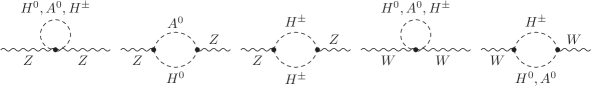
Figure 1: Non-standard contributions from the THDM scalars to the $Z$ and $W$ boson self-energies in the alignment limit at the one-loop level.

The calculation of the effective coupling strengths at the one-loop order in the gauge-less limit results in

$$\frac{G_{NC}}{\sqrt{2}}=\frac{e_{0}^{2}}{8s_{W,0}^{2}c_{W,0}^{2}M_{Z,0}^{2}}\left[1+\frac{\Sigma^{(1)}_{Z}\left(0\right)}{M_{Z}^{2}}\right]$$ (116)

and

$$\frac{G_{CC}}{\sqrt{2}}=\frac{e_{0}^{2}}{8s_{W,0}^{2}M_{W,0}^{2}}\left[1+\frac{\Sigma^{(1)}_{W}\left(0\right)}{M_{W}^{2}}\right].$$ (117)

The expansion of the bare parameters cancel in the $\rho$ parameter. Therefore, the correction to the $\rho$ parameter at one-loop order is given by

$$\Delta\rho^{(1)}=\frac{\Sigma^{(1)}_{Z}\left(0\right)}{M_{Z}^{2}}-\frac{\Sigma^{(1)}_{W}\left(0\right)}{M_{W}^{2}}.$$ (118)

In the THDM with the assumptions described in section 3 we can split the one-loop correction

$$\Delta\rho^{(1)}=\Delta\rho_{\text{t}}^{\text{(1)}}+\Delta\rho_{\text{NS}}^{\text{(1)}}$$ (119)

into two independent parts originating from the top-Yukawa coupling and the scalar sector. The first part arises from the large mass splitting between the top and the bottom quark and is identical to the dominant part of the one-loop corrections to $\Delta\rho$ in the SM Veltman:1977kh ; Chanowitz:1978mv ; Chanowitz:1978uj . When neglecting the mass of the bottom quark one obtains the one-loop result

$$\Delta\rho_{\text{t}}^{\text{(1)}}=\frac{3\alpha_{\text{em}}}{16\pi M_{W}^{2}s_{W}^{2}}m_{t}^{2}.$$ (120)

In the SM no contributions to $\Delta\rho^{(1)}$ arise from scalar loops due to the custodial symmetry of the Higgs potential. In a similar way there is no correction from the SM-like scalars $h^{0}$, $G^{0}$ and $G^{\pm}$ in the THDM with the assumptions from section 3, since the part $V_{I}$ of the potential in (50) is custodial invariant. The contributions from the SM-like scalars to the gauge-boson self-energies yield the SM result in dimensional regularization with dimension $D$, expressed in terms of $A_{0}$ in B.1,

$$\frac{\Sigma^{(1)}_{V,\text{SM}}\left(0\right)}{M_{V}^{2}}=\frac{\alpha_{\text{em}}}{16\pi s_{W}^{2}M_{W}^{2}}\frac{(D-4)}{D}A_{0}\left(m_{h^{0}}^{2}\right),$$ (121)

for both $V=W,Z$. They cancel in the difference for $\Delta\rho^{(1)}$ in (118).

However, the extended scalar sector of the THDM gives additional scalar contributions to $\Delta\rho$ Bertolini:1985ia ; Hollik:1986gg ; Hollik:1987fg ; Denner:1991ie ; Grimus:2007if ; gunion:1990 . In the alignment limit the additional correction follows from the scalars $H^{0}$, $A^{0}$ and $H^{\pm}$. The gauge-boson self-energies from the diagrams in figure 1 give rise to the non-standard one-loop part

$$\Delta\rho_{\text{NS}}^{\text{(1)}}= \frac{\alpha_{\text{em}}}{16\pi s_{W}^{2}M_{W}^{2}D}\Big{\{}4m_{A^{0}}^{2}B_{0}\left(0,m_{A^{0}}^{2},m_{H^{\pm}}^{2}\right)$$

$$+4m_{H^{0}}^{2}B_{0}\left(0,m_{H^{0}}^{2},m_{H^{\pm}}^{2}\right)$$

$$-4m_{A^{0}}^{2}B_{0}\left(0,m_{A^{0}}^{2},m_{H^{0}}^{2}\right)$$

$$+(8-2D)A_{0}\left(m_{H^{\pm}}^{2}\right)-4A_{0}\left(m_{H^{0}}^{2}\right)\Big{\}}$$ (122)

which simplifies to

$$\Delta\rho_{\text{NS}}^{\text{(1)}}\xrightarrow{D\rightarrow 4} \frac{\alpha_{\text{em}}}{16\pi s_{W}^{2}M_{W}^{2}}\Bigg{\{}\frac{m_{A^{0}}^{2}m_{H^{0}}^{2}}{m_{A^{0}}^{2}-m_{H^{0}}^{2}}\log\left(\frac{m_{A^{0}}^{2}}{m_{H^{0}}^{2}}\right)$$

$$-\frac{m_{A^{0}}^{2}m_{H^{\pm}}^{2}}{m_{A^{0}}^{2}-m_{H^{\pm}}^{2}}\log\left(\frac{m_{A^{0}}^{2}}{m_{H^{\pm}}^{2}}\right)$$

$$-\frac{m_{H^{0}}^{2}m_{H^{\pm}}^{2}}{m_{H^{0}}^{2}-m_{H^{\pm}}^{2}}\log\left(\frac{m_{H^{0}}^{2}}{m_{H^{\pm}}^{2}}\right)$$

$$+m_{H^{\pm}}^{2}\Bigg{\}}.$$ (123)

in four dimensions. It increases quadratically with the mass difference between the charged and the neutral Higgs states, and it vanishes for

$$m_{H^{0}}=m_{H^{\pm}}$$ (124)

or

$$m_{A^{0}}=m_{H^{\pm}}.$$ (125)

The reason is that this correction contains only couplings between the Goldstone bosons and the non-standard scalars $H^{0}$, $A^{0}$ and $H^{\pm}$ which are determined by the part $V_{III}$ of the potential. As explained in section 4, the custodial symmetry in this part can be restored for equal charged and neutral Higgs masses. Note that in the alignment case the entire non-standard one-loop contribution to $\Delta\rho$ is exclusively given by the expression (123), corresponding to the gauge-less limit.

6.2 Higher-order corrections in the THDM

As mentioned above, it is sufficient to keep only the corrections from the gauge-boson self-energies in the calculation of the effective neutral and charged current interaction of the four fermion processes. The two-loop results of the effective couplings are

$$\frac{G_{NC}}{\sqrt{2}}= \frac{e_{0}^{2}}{8s_{W,0}^{2}c_{W,0}^{2}M_{Z,0}^{2}}\left[1+\frac{\Sigma^{(1)}_{Z}\left(0\right)}{M_{Z}^{2}}-\frac{\delta M_{Z}^{2}}{M_{Z}^{2}}\frac{\Sigma^{(1)}_{Z}\left(0\right)}{M_{Z}^{2}}\right.$$

$$\left.+\left(\frac{\Sigma^{(1)}_{Z}\left(0\right)}{M_{Z}^{2}}\right)^{2}+\frac{\Sigma^{(2)}_{Z}\left(0\right)}{M_{Z}^{2}}\right]$$ (126)

and

$$\frac{G_{CC}}{\sqrt{2}}= \frac{e_{0}^{2}}{8s_{W,0}^{2}M_{W,0}^{2}}\left[1+\frac{\Sigma^{(1)}_{W}\left(0\right)}{M_{W}^{2}}-\frac{\delta M_{W}^{2}}{M_{W}^{2}}\frac{\Sigma^{(1)}_{W}\left(0\right)}{M_{W}^{2}}\right.$$

$$\left.+\left(\frac{\Sigma^{(1)}_{W}\left(0\right)}{M_{W}^{2}}\right)^{2}+\frac{\Sigma^{(2)}_{W}\left(0\right)}{M_{W}^{2}}\right].$$ (127)

With the renormalization condition (106) for the gauge-boson mass counterterms in the gauge-less limit the products of one-loop corrections in the brackets cancel. The calculation of $\rho$ as defined by (107) then yields the deviation $\Delta\rho$ in (111) as follows,

$$\Delta\rho= \left(\frac{\Sigma^{(1)}_{Z}\left(0\right)}{M_{Z}^{2}}-\frac{\Sigma^{(1)}_{W}\left(0\right)}{M_{W}^{2}}\right)$$

$$-\frac{\Sigma^{(1)}_{Z}\left(0\right)}{M_{Z}^{2}}\left(\frac{\Sigma^{(1)}_{Z}\left(0\right)}{M_{Z}^{2}}-\frac{\Sigma^{(1)}_{W}\left(0\right)}{M_{W}^{2}}\right)$$

$$+\left(\frac{\Sigma^{(2)}_{Z}\left(0\right)}{M_{Z}^{2}}-\frac{\Sigma^{(2)}_{W}\left(0\right)}{M_{W}^{2}}\right)$$ (128)

$$= \Delta\rho^{(1)}+\Delta\rho^{(2)},$$ (129)

where the two-loop part is given by

$$\Delta\rho^{(2)}\equiv-\frac{\Sigma^{(1)}_{Z}\left(0\right)}{M_{Z}^{2}}\Delta\rho_{\text{}}^{\text{(1)}}+\left(\frac{\Sigma^{(2)}_{Z}\left(0\right)}{M_{Z}^{2}}-\frac{\Sigma^{(2)}_{W}\left(0\right)}{M_{W}^{2}}\right).$$ (130)

$\Delta\rho^{(1)}$ summarizes the one-loop corrections as given by (118) and (119). The self-energy of the $Z$ boson in the first term consists of all the corrections from the top quark and the scalars as internal particles. Note that it contains also the part from the SM-like scalars in (121), which cancel in $\Delta\rho_{\text{}}^{\text{(1)}}$. The second part of (130) follows from the two-loop corrections to the gauge-boson self-energies. In addition to the part from the genuine two-loop diagrams (labeled as $\delta\rho_{\text{}}^{\text{(2Loop)}}$) it also includes one-loop diagrams with counterterm insertions for the subloop renormalization (labeled as $\Delta\rho_{\text{}}^{\text{(CT)}}$).

With the assumptions from section 3 we have two sources for the two-loop contribution $\Delta\rho_{\text{}}^{\text{(2)}}$: the top-Yukawa interaction and the scalar self-interaction. Due to the alignment limit we can subdivide the top-Yukawa corrections into two parts. The first one is identical to the two-loop top-Yukawa contribution in the SM and is discussed in section 6.2.1. The second one originates from the coupling between the top quark and the non-standard scalars $H^{0}$, $A^{0}$ and $H^{\pm}$ and is described in more detail in section 6.2.2. A similar separation can be made for the additional corrections to the $\rho$ parameter from the scalar self-interaction. The part $V_{I}$ of the potential (see (51)), which describes only the interaction between $h^{0}$ and the Goldstone bosons $G^{0}$, $G^{\pm}$, is invariant under the custodial symmetry and the corresponding contributions to the vector-boson self-energies in $\Delta\rho$ cancel each other. The remaining part of the potential gives rise to two finite subsets in $\Delta\rho_{\text{}}^{\text{(2)}}$. One follows from the interaction between the SM-like scalars $h^{0}$, $G^{0}$, $G^{\pm}$ and the non-standard scalars $H^{0}$, $A^{0}$, $H^{\pm}$ and is discussed in section 6.2.4. The other one contains only the non-standard scalars $H^{0}$, $A^{0}$ and $H^{\pm}$ as internal particles in the gauge-boson self-energies and is described in section 6.2.3.

With this categorization we subdivide the contribution from the genuine two-loop diagrams (without subloop renormalization) to the vector-boson self-energies into different parts, according to their origin,

$$\delta\rho_{\text{}}^{\text{(2Loop)}}=\delta\rho_{\text{t,SM}}^{\text{(2Loop)}}+\delta\rho_{\text{t,NS}}^{\text{(2Loop)}}\\ +\delta\rho_{\text{H,NS}}^{\text{(2Loop)}}+\delta\rho_{\text{H,Mix}}^{\text{(2Loop)}}$$ (131)

which are classified by the participating couplings:

• $\delta\rho_{\text{t,SM}}^{\text{(2Loop)}}$ originates from the coupling between the top quark and the SM-like scalars $h^{0}$, $G^{0}$ and $G^{\pm}$ (see section 6.2.1);

• $\delta\rho_{\text{t,NS}}^{\text{(2Loop)}}$ is the part which follows from the top-Yukawa interaction of the non-standard scalars $H^{0}$, $A^{0}$ and $H^{\pm}$ (see section 6.2.2);

• $\delta\rho_{\text{H,NS}}^{\text{(2Loop)}}$ contains the scalar self-coupling between the non-standard scalars (see section 6.2.3);

• $\delta\rho_{\text{H,Mix}}^{\text{(2Loop)}}$ follows from the interaction between the SM-like scalars and the non-standard scalars (see section 6.2.4).

Figure 2: Generic diagrams for the gauge-boson self-energies containing quarks with counterterm insertions. $V=\{W,Z\}$; $f,f^{\prime}=\{t,b\}$.

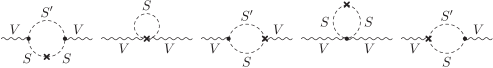
Figure 3: Generic diagrams for the gauge-boson self-energies $V=\{W,Z\}$ containing scalars with counterterm insertions. The contribution from the diagrams can be divided into two parts: one part with only the SM-like scalars ($S,S^{\prime}=\{h^{0},G^{0},G^{\pm}\}$) and one part with only the non-standard scalars ($S,S^{\prime}=\{H^{0},A^{0},H^{\pm}\}$).

For one-loop subrenormalization we need the diagrams shown in figure 2 for the self-energies with the top quarks and in figure 3 for the scalar contribution. In the gauge-less limit only two types of renormalization constants survive: the counterterm $\delta s_{W}^{2}$ from the counterterm insertions in the vertices, and the mass counterterms in the propagators of the internal particles. All field counterterms of the internal particles drop out in the calculation, and all other counterterms are zero in the gauge-less limit.

From the diagrams of figure 2 we obtain the part of the subloop renormalization from the top quark. The renormalization of the weak mixing angle is contained in the vertex counterterms (see A) and yields the term

$$\frac{s_{W}^{2}}{c_{W}^{2}}\frac{\delta s_{W}^{2}}{s_{W}^{2}}\frac{\Sigma^{(1)}_{Z,\text{t}}\left(0\right)}{M_{Z}^{2}}-\frac{\delta s_{W}^{2}}{s_{W}^{2}}\Delta\rho_{\text{t}}^{\text{(1)}}.$$ (132)

From the diagrams with counterterms in the propagators in figure 2 we obtain the term

$$\delta\rho_{\text{t}}^{\text{(CT)}}=-\frac{3\alpha_{\text{em}}(D-4)(D-2)^{2}A_{0}\left(m_{t}^{2}\right)}{16\pi DM_{W}^{2}s_{W}^{2}}\frac{\delta m_{t}}{m_{t}}.$$ (133)

Due to the alignment limit we can split the result of the top mass counterterm into a SM-like and a non-standard part. We use this for the seperation

$$\delta\rho_{\text{t}}^{\text{(CT)}}=\delta\rho_{\text{t,SM}}^{\text{(CT)}}+\delta\rho_{\text{t,NS}}^{\text{(CT)}}\,,$$ (134)

where the two parts are defined as follows:

• the part $\delta\rho_{\text{t,SM}}^{\text{(CT)}}$ contains the correction to the top-mass counterterm from the SM-like scalars $h^{0}$, $G^{0}$, $G^{\pm}$ as shown in the self-energy diagrams in figure 5;

• the second part $\delta\rho_{\text{t,NS}}^{\text{(CT)}}$ contains the part of $\delta m_{t}$ which comes from the top quark self-energy corrections from the non-standard scalars as depicted in figure 6.

For the subloop renormalization diagrams in figure 3 with the SM-like scalars $h^{0}$, $G^{0}$ and $G^{\pm}$ we find that the mass counterterms drop out in the difference of the $W$ and $Z$ self-energy, due to custodial symmetry. From the vertex counterterms we obtain the contribution

$$\frac{s_{W}^{2}}{c_{W}^{2}}\frac{\delta s_{W}^{2}}{s_{W}^{2}}\frac{\Sigma^{(1)}_{Z,\text{SM}}\left(0\right)}{M_{Z}^{2}}$$ (135)

with the one-loop self-energy from (121).

The diagrams in figure 3 with the possible insertions of the non-standard scalars for $S$ and $S^{\prime}$ give the last part of the subloop renormalization. With the Feynman rules of A the counterterms in the vertices yield the contribution

$$\frac{\Sigma^{(1)}_{Z,\text{NS}}\left(0\right)}{M_{Z}^{2}}\frac{s_{W}^{2}}{c_{W}^{2}}\frac{\delta s_{W}^{2}}{s_{W}^{2}}-\frac{\delta s_{W}^{2}}{s_{W}^{2}}\Delta\rho_{\text{NS}}^{\text{(1)}},$$ (136)

where the $Z$ self-energy in the first term contains just the contribution of the non-standard scalars.

The correction from the mass counterterms $\delta m_{H^{0}}^{2}$, $\delta m_{A^{0}}^{2}$ and $\delta m_{H^{\pm}}^{2}$ in the diagrams in figure 3 is denoted by $\delta\rho_{\text{H}}^{\text{(CT)}}$. It is identical to

$$\delta\rho_{\text{H}}^{\text{(CT)}}=\Big{(} \delta m_{A^{0}}^{2}\frac{\partial}{\partial m_{A^{0}}^{2}}+\delta m_{H^{0}}^{2}\frac{\partial}{\partial m_{H^{0}}^{2}}$$ (137)

$$+\delta m_{H^{\pm}}^{2}\frac{\partial}{\partial m_{H^{\pm}}}\Big{)}\Delta\rho_{\text{1}}^{\text{(NS)}},$$

with the one-loop contribution from (122). By splitting up the mass counterterms we will classify three different parts

$$\delta\rho_{\text{H}}^{\text{(CT)}}=\delta\rho_{\text{H,t}}^{\text{(CT)}}+\delta\rho_{\text{H,NS}}^{\text{(CT)}}+\delta\rho_{\text{H,Mix}}^{\text{(CT)}}\,,$$ (138)

which are defined as follows:

• $\delta\rho_{\text{H,t}}^{\text{(CT)}}$ contains the non-standard scalar mass counterterms originating from the top-Yukawa coupling. The corresponding diagrams are shown in figure 7.

• $\delta\rho_{\text{H,NS}}^{\text{(CT)}}$ labels the part which contains only non-standard scalars in the calculation of $\delta m_{H^{0}}^{2}$, $\delta m_{A^{0}}^{2}$ and $\delta m_{H^{\pm}}^{2}$. The diagrams are displayed in figure 9.

• $\delta\rho_{\text{H,Mix}}^{\text{(CT)}}$ incorporates the contribution to the mass counterterms of $H^{0}$, $A^{0}$ and $H^{\pm}$ which originates from the couplings of the non-standard scalars to the SM-like scalars. The corresponding self-energy diagrams are presented in figure 11.

When we combine the various parts from the subloop renormalization, their overall contribution to $\Delta\rho_{\text{}}^{\text{(2)}}$ can be written as follows:

$$\Delta\rho_{\text{}}^{\text{(CT)}}= \frac{s_{W}^{2}}{c_{W}^{2}}\frac{\delta s_{W}^{2}}{s_{W}^{2}}\frac{\Sigma^{(1)}_{Z}\left(0\right)}{M_{Z}^{2}}$$ (139)

$$-\frac{\delta s_{W}^{2}}{s_{W}^{2}}\left(\Delta\rho_{\text{t}}^{\text{(1)}}+\Delta\rho_{\text{NS}}^{\text{(1)}}\right)+\delta\rho_{\text{}}^{\text{(CT)}}.$$

The first term incorporates all parts from (132), (135) and (136) involving a single $Z$-boson self-energy; the remaining terms from the renormalization of $s_{W}$ in (132) and (136) are kept separately in the second term. The last term

$$\delta\rho_{\text{}}^{\text{(CT)}}=\delta\rho_{\text{t}}^{\text{(CT)}}+\delta\rho_{\text{H}}^{\text{(CT)}}$$ (140)

collects the various parts resulting from the mass counterterms of the internal particles.

The two-loop correction to the $\rho$ parameter in (130) can be further simplified, since the counterterm of the weak mixing angle reduces to

$$\frac{\delta s_{W}^{2}}{s_{W}^{2}}=\frac{c_{W}^{2}}{s_{W}^{2}}\left(\frac{\Sigma^{(1)}_{Z}\left(0\right)}{M_{Z}^{2}}-\frac{\Sigma^{(1)}_{W}\left(0\right)}{M_{W}^{2}}\right)=\frac{c_{W}^{2}}{s_{W}^{2}}\Delta\rho_{\text{}}^{\text{(1)}}{}.$$ (141)

in the gauge-less limit (see (106)). Combined with (139) the first term in (130) is canceled and we obtain

$$\Delta\rho^{(2)}=-\frac{c_{W}^{2}}{s_{W}^{2}}\left(\Delta\rho_{\text{}}^{\text{(1)}}\right)^{2}+\delta\rho_{\text{}}^{\text{(2)}}.$$ (142)

In this notation, the genuine two-loop part

$$\delta\rho_{\text{}}^{\text{(2)}}=\delta\rho_{\text{}}^{\text{(CT)}}+\delta\rho_{\text{}}^{\text{(2Loop)}}$$ (143)

contains $\delta\rho_{\text{}}^{\text{(CT)}}$ resulting exclusively from the insertions of the mass counterterms, and the contribution $\delta\rho_{\text{}}^{\text{(2Loop)}}$ from the pure two-loop diagrams for the $Z,W$ self-energies (without subloop renormalization) in (130).

The appearance of the reducible term $\left(\Delta\rho_{\text{}}^{\text{(1)}}\right)^{2}$ in $\Delta\rho_{\text{}}^{\text{(2)}}$ is a consequence of the parameterisation of $v^{2}$ by

$$\frac{1}{v^{2}}=\frac{e^{2}}{4s_{W}^{2}M_{W}^{2}}$$ (144)

together with the on-shell renormalization of $s_{W}$. A different parameterisation in terms of the Fermi constant $G_{F}$ can be introduced with the help of the relation

$$\sqrt{2}G_{F}=\frac{e^{2}}{4M_{W}^{2}s_{W}^{2}}\left(1+\Delta r\right),$$ (145)

where the quantity $\Delta r$ describes the higher-order corrections. In the gauge-less limit the one-loop contribution is given by

$$\Delta r=-\frac{\delta s_{W}^{2}}{s_{W}^{2}}.$$ (146)

Consequently, the reparameterisation of the one-loop result $\Delta\rho_{\text{}}^{\text{(1)}}$ in terms of $G_{F}$ induces a two-loop shift originating from $\Delta r$, which effectively cancels the reducible term in $\Delta\rho_{\text{}}^{\text{(2)}}$ in (142). Hence, in the $G_{F}$ expansion, the two-loop contribution in $\Delta\rho$ is identified as the irreducible two-loop part $\delta\rho^{(2)}$ in (143). In this way, the same pattern for $\rho$ is found as in the SM Consoli:1989fg .

The structure of the irreducible quantity $\delta\rho^{(2)}$ in (143) with $\delta\rho^{({\rm 2Loop})}$ defined in (131) allows us to divide it into four finite subsets of different origins,

$$\delta\rho^{(2)}=\delta\rho^{(2)}_{\rm t,SM}+\delta\rho^{(2)}_{\rm t,NS}+\delta\rho^{(2)}_{\rm H,NS}+\delta\rho^{(2)}_{\rm H,Mix}\,,$$ (147)

which we describe now in more detail.

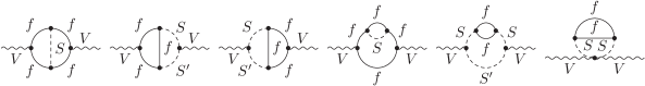
Figure 4: Generic two-loop diagrams for the top-Yukawa corrections to the vector-boson self-energies with $V=\{W,Z\}$ and $f=\{t,b\}$. The standard contribution $\delta\rho_{\text{t,SM}}^{\text{(2Loop)}}$ follows from $S,S^{\prime}=\{h^{0},G^{0},G^{\pm}\}$. The non-standard contribution $\delta\rho_{\text{t,NS}}^{\text{(2Loop)}}$ is obtained by all possible insertions of $S,S^{\prime}=\{H^{0},A^{0},H^{\pm}\}$.

6.2.1 Standard model corrections from the top-Yukawa coupling

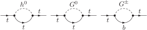
Figure 5: One-loop diagrams for the standard contribution to the top-mass counterterm $\delta m_{t}$.

The first contribution under investigation are the two-loop corrections from the top-Yukawa coupling. In the alignment limit this corrections can be split into two independent subsets. From the coupling of the top quark to the SM-like scalars $h^{0}$, $G^{0}$ and $G^{\pm}$ we obtain the finite correction

$$\delta\rho_{\text{t,SM}}^{\text{(2)}}=\delta\rho_{\text{t,SM}}^{\text{(CT)}}+\delta\rho_{\text{t,SM}}^{\text{(2Loop)}}.$$ (148)

$\delta\rho_{\text{t,SM}}^{\text{(2Loop)}}$ are the pure two-loop contributions, which are depicted by the generic diagrams in figure 4 for $S,S^{\prime}={h^{0},G^{0},G^{\pm}}$. Its divergences are cancelled by the part $\delta\rho_{\text{t,SM}}^{\text{(CT)}}$ which is the part of (133) with the top-mass counterterm calculated from the diagrams in figure 5. $\delta\rho_{\text{t,SM}}^{\text{(2)}}$ is identical to the already known SM contribution from the top-Yukawa interaction. First the result was calculated in the approximation $M_{H}=0$ vanderBij:1986hy and as an expansion for large values of $M_{H}$ vanderBij:1983bw . Later the full result for arbitrary Higgs masses was obtained Barbieri:1992dq ; Fleischer:1993ub ; Fleischer:1994cb . We checked that our calculation leads to the same result.

6.2.2 Non-standard corrections from the top-Yukawa coupling

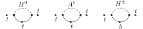
Figure 6: One-loop diagrams for the non-standard contribution to the top-mass counterterm $\delta m_{t}$.

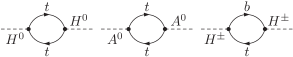
Figure 7: One-loop diagrams for the top-Yukawa contribution to the non-standard scalar mass counterterms.

More interesting is the additional contribution due to the coupling of the top quark to the non-standard scalars $H^{0}$, $A^{0}$ and $H^{\pm}$, which is given by

$$\delta\rho_{\text{t,NS}}^{\text{(2)}}=\delta\rho_{\text{t,NS}}^{\text{(CT)}}+\delta\rho_{\text{H,t}}^{\text{(CT)}}+\delta\rho_{\text{t,NS}}^{\text{(2Loop)}}.$$ (149)

$\delta\rho_{\text{t,NS}}^{\text{(2Loop)}}$ denotes the pure two-loop part, represented by the generic diagrams shown in figure 4 with $S,S^{\prime}=\{H^{0},A^{0},H^{\pm}\}$. The result does not only consist of terms of $\mathcal{O}\left(\alpha_{t}^{2}\right)$, which originate only from the top-Yukawa interaction, but also of contributions of $\mathcal{O}\left(\alpha_{t}\lambda_{i}\right)$ which contain the scalar self-couplings in addition to the top-Yukawa coupling. The divergences from the $\mathcal{O}\left(\alpha_{t}^{2}\right)$ part are canceled by $\delta\rho_{\text{t,NS}}^{\text{(CT)}}$ which originates from the subloop renormalization diagrams of figure 2 with the top-mass counterterm calculated from the diagrams in figure 6. The divergences of $\mathcal{O}\left(\alpha_{t}\lambda_{i}\right)$ are cancelled by $\delta\rho_{\text{H,t}}^{\text{(CT)}}$ with the mass counterterms calculated from the diagrams in figure 7. In the calculation by means of the gauge-boson self-energies the separation between the $\mathcal{O}\left(\alpha_{t}^{2}\right)$ and the $\mathcal{O}\left(\alpha_{t}\lambda_{i}\right)$ contributions is obscured. Using the Ward identity in (114) can help to disentangle the two different finite contributions of $\mathcal{O}\left(\alpha_{t}^{2}\right)$ and $\mathcal{O}\left(\alpha_{t}\lambda_{i}\right)$.

6.2.3 Scalar corrections from the interaction of the non-standard scalars

Figure 8: Generic two-loop diagrams for the vector-boson self-energies from the interaction from the non-standard scalars. $V=\{W,Z\}$; $S=\{H^{0},A^{0},H^{\pm}\}$.

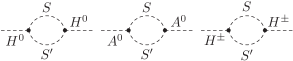
Figure 9: One-loop diagrams for the non-standard scalar mass counterterms from the interaction between the non-standard scalars. For the $H^{0}$ self-energy: $S=S^{\prime}=H^{0},A^{0},H^{\pm}$. For the $A^{0}$ self-energy: $S=A^{0}$ and $S^{\prime}=H^{0}$. For the $H^{\pm}$ self-energy: $S=H^{\pm}$ and $S^{\prime}=H^{0}$.

The interaction between the non-standard scalars gives another finite subset. When inspecting this contribution we found that all the corrections from a coupling between four non-standard scalars are cancelled. The two-loop diagrams which contain such a coupling can be written as a product of two scalar one-loop integrals. The mass counterterms in the subloop renormalization lead to the same product from the corrections to the scalar self-energies, but with an opposite sign. Consequently the two terms cancel each other.

The remaining contribution

$$\delta\rho_{\text{H,NS}}^{\text{(2)}}=\delta\rho_{\text{H,NS}}^{\text{(CT)}}+\delta\rho_{\text{H,NS}}^{\text{(2Loop)}}$$ (150)

comes from all the diagrams which include a triple scalar coupling between $H^{0}$, $A^{0}$ and $H^{\pm}$. $\delta\rho_{\text{H,NS}}^{\text{(2Loop)}}$ is the result for the vector-boson self-energies of the generic two-loop diagrams in figure 8. For the subloop renormalization we need the corrections from the triple non-standard scalar coupling to the scalar self-energies, as shown in figure 9. Inserting the corresponding mass counterterms into (137) leads to the result of $\delta\rho_{\text{H,NS}}^{\text{(CT)}}$.

6.2.4 Scalar corrections from the interaction of the non-standard scalars with the SM scalars

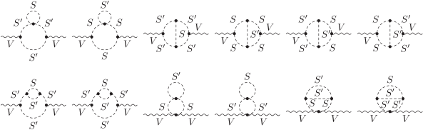
Figure 10: Generic two-loop diagrams from the interaction between the SM-like scalars $S=h^{0}$, $G^{0}$, $G^{\pm}$ and the non-standard scalars $S^{\prime}=H^{0}$, $A^{0}$, $H^{\pm}$. $V=\{W,Z\}$

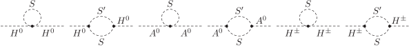
Figure 11: One-loop diagrams for the non-standard scalar mass counterterms from the interaction between the SM-like scalars $S=h^{0},G^{0},G^{\pm}$ and the non-standard scalars $S^{\prime}=H^{0},A^{0},H^{\pm}$.

As already mentioned another finite subset of two-loop corrections to the $\rho$ parameter comes from the interaction between the scalars $h^{0}$, $G^{0}$, $G^{\pm}$ with the non-standard scalars $H^{0}$, $A^{0}$, $H^{\pm}$. This interaction follows only from the part $V_{III}$ of the potential (see (53)) which is custodial-symmetry breaking. We denote the resulting contribution by

$$\delta\rho_{\text{H,Mix}}^{\text{(2)}}=\delta\rho_{\text{H,Mix}}^{\text{(CT)}}+\delta\rho_{\text{H,Mix}}^{\text{(2Loop)}},$$ (151)

where $\delta\rho_{\text{H,Mix}}^{\text{(2Loop)}}$ is the part from the two-loop diagrams shown in figure 10. The divergences are canceled by $\delta\rho_{\text{H,Mix}}^{\text{(CT)}}$ from (138), which is obtained by calculating the mass counterterms in (137) from the diagrams in figure 11.

6.3 The Inert-Higgs-Doublet model

We now discuss our result in the context of a special version of the THDM, the Inert-Higgs-Doublet Model (IHDM). Originally proposed in Deshpande:1977rw , it has received topical attention in the light of neutrino mass phenomenology and dark-matter searches (see e.g. Arhrib:2013ela for a recent comprehensive analysis and more references). In the IHDM the SM scalar sector is extended by a second complex doublet with the special feature that the Lagrangian has an exact $Z_{2}$ symmetry under which all the SM particles are even while the second doublet is odd. This $Z_{2}$ symmetry has several interesting consequences. The requirement that it stays unbroken forbids a vacuum expectation value of the second doublet. Therefore the doublets of the IHDM are

$$H_{1}= \begin{pmatrix}G^{\pm}\\ \frac{1}{\sqrt{2}}\left(v+h^{0}+iG^{0}\right)\end{pmatrix},$$ (152)

$$H_{2}= \begin{pmatrix}H^{\pm}\\ \frac{1}{\sqrt{2}}\left(H^{0}+iA^{0}\right)\end{pmatrix}.$$ (153)

The doublet $H_{1}$ is identical to the scalar doublet in the SM. It consists of the physical SM-like Higgs boson $h^{0}$ and the Goldstone bosons $G^{0}$ and $G^{\pm}$. The second doublet $H_{2}$ transforms under the $Z_{2}$ as $H_{2}\rightarrow-H_{2}$ and contains the $CP$-even scalar $H^{0}$, the $CP$-odd scalar $A^{0}$ and the charged scalars $H^{\pm}$. All the terms in the Lagrangian in which the SM particles couple to a single scalar of $H_{2}$ are forbidden by the $Z_{2}$ symmetry and the lightest of the scalars from $H_{2}$ is stable. If this is one of the neutral states $H^{0}$ or $A^{0}$ the IHDM provides a dark matter candidate.

The most general scalar potential which is renormalizable, gauge invariant and respects the $Z_{2}$ symmetry is given by (see for example Arhrib:2015hoa )

$$V^{\text{IHDM}}= \mu_{1}^{2}\left(H_{1}^{\dagger}H_{1}\right)+\mu_{2}^{2}\left(H_{2}^{\dagger}H_{2}\right)+\Lambda_{1}\left(H_{1}^{\dagger}H_{1}\right){}^{2}$$

$$+\Lambda_{2}\left(H_{2}^{\dagger}H_{2}\right){}^{2}+\Lambda_{3}\left(H_{2}^{\dagger}H_{2}\right)\left(H_{1}^{\dagger}H_{1}\right)$$

$$+\Lambda_{4}\left(H_{1}^{\dagger}H_{2}\right)\left(H_{2}^{\dagger}H_{1}\right)$$

$$+\frac{1}{2}\Lambda_{5}\left(\left(H_{1}^{\dagger}H_{2}\right){}^{2}+\left(H_{2}^{\dagger}H_{1}\right){}^{2}\right).$$ (154)

To avoid $CP$-violation all the parameters in the potential are chosen to be real. The minimization condition can be used to eliminate one of the parameters from the potential. From the remaining six parameters four can be expressed by the scalar masses (see Arhrib:2015hoa for the explicit relations between the masses and the potential parameters). If we choose $\mu_{2}^{2}$ and $\Lambda_{2}$ for the remaining two parameters we can express the potential by

$$V^{\text{IHDM}}= V^{\text{IHDM}}_{I}+V^{\text{IHDM}}_{II}+V^{\text{IHDM}}_{III},$$ (155)

$$V^{\text{IHDM}}_{I}= \frac{m_{h^{0}}^{2}}{2v^{2}}\left(H_{1}^{\dagger}H_{1}\right){}^{2}-\frac{1}{2}m_{h^{0}}^{2}\left(H_{1}^{\dagger}H_{1}\right),$$ (156)

$$V^{\text{IHDM}}_{II}= \mu_{2}^{2}\left(H_{2}^{\dagger}H_{2}\right)+\Lambda_{2}\left(H_{2}^{\dagger}H_{2}\right){}^{2},$$ (157)

$$V^{\text{IHDM}}_{III}= \frac{\left(m_{A^{0}}^{2}-2m_{H^{\pm}}^{2}+m_{H^{0}}^{2}\right)}{v^{2}}\left(H_{1}^{\dagger}H_{2}\right)\left(H_{2}^{\dagger}H_{1}\right)$$

$$+\frac{\left(m_{H^{0}}^{2}-m_{A^{0}}^{2}\right)}{2v^{2}}\left[\left(H_{1}^{\dagger}H_{2}\right){}^{2}+\left(H_{2}^{\dagger}H_{1}\right){}^{2}\right]$$

$$+\frac{2\left(m_{H^{\pm}}^{2}-\mu_{2}^{2}\right)}{v^{2}}\left(H_{1}^{\dagger}H_{1}\right)\left(H_{2}^{\dagger}H_{2}\right).$$ (158)

We see that the SM-like doublet $\Phi_{\text{SM}}$ in the aligned THDM is identical to the doublet $H_{1}$ in the IHDM. The non-standard doublet $\Phi_{\text{NS}}$ in (46) differs from the doublet $H_{2}$ of the IHDM by the overall sign in front of the $CP$-even scalar $H^{0}$. However, our result is independent on this overall sign, since the $CP$-even scalar $H^{0}$ appears only as an internal particle in the calculated self-energies. Therefore we can identify the doublet $H_{2}$ with the doublet $\Phi_{\text{NS}}$. By using this identifications we can relate the potential between the IHDM and the more general THDM in the alignment limit in order to interpret our results in the context of the IHDM:

• There is no non-standard correction to $\Delta\rho$ from the top-Yukawa interaction, since the interaction of the fermions with the non-standard scalars is forbidden by the $Z_{2}$ symmetry.

• The part $V^{\text{IHDM}}_{I}$ has the same structure as the scalar potential of the SM and will not lead to contributions to the $\rho$ parameter since it is invariant under the custodial symmetry (see section 4).

• In the IHDM all the quartic couplings between four non-standard scalars are proportional to $\Lambda_{2}$. However, in our calculation in the aligned THDM we found that all the contributions to $\Delta\rho$ from couplings between four non-standard scalars vanish (see section 6.2.3). The responsible arguments can also be transferred to the IHDM.

• When we identify $H_{1}$ with $\Phi_{\text{SM}}$ and $H_{2}$ with $\Phi_{\text{NS}}$ we see that the part $V_{III}$ of the potential in the aligned THDM can be obtained by the replacement

  $$\mu_{2}^{2}=\frac{1}{2}\lambda_{5}v^{2}-\frac{m_{h^{0}}^{2}}{2}$$ (159)

  in $V^{\text{IHDM}}_{III}$. Consequently for the calculation of the $\rho$ parameter in the IHDM we get corrections corresponding to $\Delta\rho_{\text{NS}}^{\text{(1)}}$ and $\delta\rho_{\text{H,Mix}}^{\text{(2)}}$. The one-loop correction $\Delta\rho_{\text{NS}}^{\text{(1)}}$ is identical in the IHDM since it is independent of $\lambda_{5}$. The two-loop part $\delta\rho_{\text{H,Mix}}^{\text{(2)}}$ can be written in terms of the IHDM parameter $\mu_{2}^{2}$ by using (159).

• As mentioned in section 6.2.3, the correction $\delta\rho_{\text{H,NS}}^{\text{(2)}}$ contains the interaction between three of the non-standard scalars $H^{0}$, $A^{0}$ and $H^{\pm}$ which follows from the part $V_{IV}$ of the potential in (50). In the IHDM couplings between three non-standard scalars are forbidden because of the exact $Z_{2}$ symmetry. As a consequence, corrections to the $\rho$ parameter which would correspond to $\delta\rho_{\text{H,NS}}^{\text{(2)}}$ are absent in the IHDM.

7 Numerical results

In this part we present the numerical results of the two-loop corrections to the $\rho$ parameter. We study the dependence on the various parameters of the aligned THDM and compare the non-standard two-loop contributions with the one-loop result which is part of existing calculations of electroweak precision observables so far. In this way the parameter regions emerge where the one-loop calculations are insufficient and bounds on parameters derived from experimental precision data will be significantly changed when the two-loop terms are taken into account. The values for the SM input parameters are Olive:2016xmw

$$M_{W}= 80.385\text{ GeV},$$ (160)

$$M_{Z}= 91.1876\text{ GeV},$$ (161)

$$m_{t}= 173.21\text{ GeV}.$$ (162)

For the mass of the SM-like Higgs state $h^{0}$ we take over the value $m_{h^{0}}=125\,\text{GeV}$.

The effect of non-standard corrections to electroweak observables is often parametrized in terms of the parameter set $S$, $T$, $U$, originally defined in Peskin:1990zt ; Peskin:1991sw . Following the conventions of Olive:2016xmw , the quantity $T$ is related to the correction $\Delta\rho$ via

$$\Delta\rho=\hat{\alpha}\left(M_{Z}\right)T$$ (163)

with the running electromagnetic fine structure constantOlive:2016xmw

$$\hat{\alpha}\left(M_{Z}\right)^{-1}=127.950\pm 0.017\,.$$ (164)

The current value of $T$  Olive:2016xmw , determined from experimental data,

$$T=0.08\pm 0.12\,,$$ (165)

can be translated into bounds for $\Delta\rho$ according to

$$-0.000313\leq\Delta\rho\leq 0.00156,$$ (166)

which can be used for a quick estimate of the effect of the higher-order contributions to $\Delta\rho$ in view of current experimental constraints.

7.1 Results for the top-Yukawa contribution

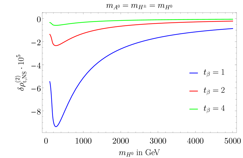
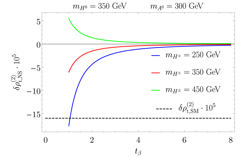
Figure 12: Analysis of $\delta\rho_{\text{t,NS}}^{\text{(2)}}$. The upper panel presents a variation of the degenerate masses $m_{H^{0}}$, $m_{A^{0}}$ and $m_{H^{\pm}}$ up to large values. The solid lines correspond to different values of $t_{\beta}$. In the lower panel $\delta\rho_{\text{t,NS}}^{\text{(2)}}$ is plotted as a function of $t_{\beta}$ for different values of $m_{H}^{\pm}$. The masses of $H^{0}$ and $A^{0}$ are fixed at $m_{H^{0}}=350\text{ GeV}$ and $m_{A^{0}}=300\text{ GeV}$. The value of the two-loop top-Yukawa correction in the SM, $\delta\rho^{(2)}_{\rm t,SM}=-1.60\cdot 10^{-4}$, is shown by the black dashed line for comparison.

We start with the analysis of the contribution $\delta\rho_{\text{t,NS}}^{\text{(2)}}$ which is originating from the coupling between the top quark and the non-standard scalars. As a first test of our result we examine the behaviour in the so-called decoupling limit Gunion:2002zf , in which the masses of the non-standard scalars are much larger than $m_{h}^{0}$. In this limit the scalar sector of the THDM can be described by an effective theory which is identical to the SM Higgs sector. Consequently we expect $\delta\rho_{\text{t,NS}}^{\text{(2)}}$ to vanish for large, equal non-standard Higgs masses. The decoupling scenario is investigated in the upper panel of figure 12, where $\delta\rho_{\text{t,NS}}^{\text{(2)}}$ is shown for degenerate masses of the non-standard scalars. The solid lines represent results for different values of $t_{\beta}$. Since the top-Yukawa coupling breaks the custodial symmetry this contribution is still non-zero, even if the custodial symmetry in the Higgs potential is restored by equal masses of the charged and neutral Higgs states. As expected it approaches zero when the masses increase. Moreover, we can see that larger values of $t_{\beta}$ suppress the correction. The reason is that the coupling of the top quark to the scalars $H^{0}$, $A^{0}$ and $H^{\pm}$ scales with $t_{\beta}^{-1}$ in the alignment limit (see section 3.2).

The influence of $t_{\beta}$ is visualised on the lower panel of figure 12 with $\delta\rho_{\text{t,NS}}^{\text{(2)}}$ for the mass configurations as described by the legend, showing the decrease of the contribution with $t_{\beta}$. In addition different mass splittings between charged and neutral scalars yield noticable deviations in the result and can even lead to different signs. In general, the top-Yukawa contribution is of the order of the SM value $\delta\rho^{(2)}_{\rm t,SM}$ or smaller.

In order to test the validity of the top-Yukawa approximation, we repeated our calculation including also the contribution from the bottom-Yukawa coupling. In the THDM of type-I and type-X the additional corrections from the bottom-Yukawa coupling are negligibly small, as expected from their suppression by the $b$-quark mass (see section 3). In the type-II and type-Y models, the contribution from the bottom-Yukawa coupling can be enhanced for large values of $t_{\beta}$ since the coupling of the $b$-quark to the non-standard scalars carries a factor $t_{\beta}$ in the alignment limit. Additional two-loop contributions from finite $m_{b}$ that reach the level of $\delta\rho_{\text{t,SM}}^{\text{(2)}}$, require $t_{\beta}\simeq 40-50$. For such large values of $t_{\beta}$, however, one has to prevent the non-standard scalar self-couplings from becoming non-perturbative by restricting the parameter $\lambda_{5}$ to be very close to $\lambda_{5}v^{2}=2m_{H^{0}}^{2}$Akeroyd:2000wc ; Das:2015qva . Moreover, the constraints from flavour physics give further significant restrictions for large values of $t_{\beta}$ (see for example Deschamps:2009rh ; Enomoto:2015wbn ).

7.2 Results for the non-standard scalar contribution

Figure 13: Effect of mass differences between neutral and charged scalars on $\delta\rho_{\text{H,NS}}^{\text{(2)}}$ for $\lambda_{5}=\pm 1$. The neutral masses are fixed at $m_{H^{0}}=350\text{ GeV}$ and $m_{A^{0}}=400\text{ GeV}$. The mass of $H^{\pm}$ is varied from $250\text{ GeV}$ to $500\text{ GeV}$. The solid lines represent different values of $t_{\beta}$ as explained in the legend. The blue dashed line shows the non-standard one-loop correction $\Delta\rho_{\text{NS}}^{\text{(1)}}$ for comparison. The grey area depicts the bounds from the experimental limits of the $T$ parameter.

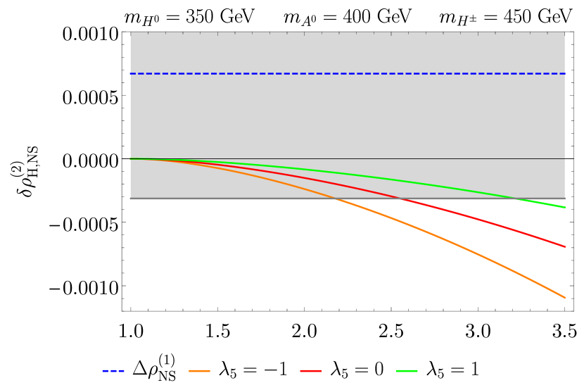
Figure 14: Influence of a variation of $t_{\beta}$ on $\delta\rho_{\text{H,NS}}^{\text{(2)}}$ for the specified mass configurations. The result is plotted for different values of $\lambda_{5}$. The blue dashed line gives the value of the non-standard one-loop correction $\Delta\rho_{\text{NS}}^{\text{(1)}}$ for the specified masses. The grey area depicts the bounds from the experimental limits of the $T$ parameter.

We now discuss the numerical results of the contribution $\delta\rho_{\text{H,NS}}^{\text{(2)}}$ which originates from the coupling between three non-standard scalars as described in section 6.2.3. The influence of a mass splitting between charged and neutral scalars is presented in figure 13. The two panels show results for $m_{H^{0}}=350\text{ GeV}$, $m_{A^{0}}=400\text{ GeV}$ and $\lambda_{5}=\pm 1$. The variation of $m_{H^{\pm}}$ is performed such that it yields similar mass differences for the specified parameter settings. The different lines correspond to different values of $t_{\beta}$ as defined in the legend. For comparison the blue dashed line displays the result for the one-loop non-standard correction $\Delta\rho_{\text{NS}}^{\text{(1)}}$. The grey area indicates the bounds from the $T$ parameter in (165).

We see that the contribution $\delta\rho_{\text{H,NS}}^{\text{(2)}}$ can give corrections to the $\rho$ parameter which are comparable in size or even larger than the one-loop correction. The reason are the new couplings between three non-standard scalars which enter for the first time in the two-loop contribution. Adding the two-loop corrections to the one-loop result can lead to noticeable modifications of the parameter region allowed by the constraints on $T$.

The triple non-standard scalar couplings arise from the term $V_{IV}$ of the potential in (50), when the vacuum expectation value

$$\langle\Phi_{\text{SM}}\rangle=\frac{1}{\sqrt{2}}\begin{pmatrix}0\\ v\end{pmatrix}$$ (167)

is inserted for the doublet $\Phi_{\text{SM}}$. Since they enter quadratically in all the diagrams in figure 8, the contribution $\delta\rho_{\text{H,NS}}^{\text{(2)}}$ is proportional to (see (54))

$$\frac{1}{4}\left(\frac{1}{t_{\beta}}-t_{\beta}\right)^{2}\left(\frac{2m_{H^{0}}^{2}}{v^{2}}-\lambda_{5}\right)^{2}.$$ (168)

The prefactor explains the strong influence of $t_{\beta}$ on the results in figure 13. The enhancement of the coupling can be weakened for positive values of $\lambda_{5}$ (see the lower panel of figure 13) or increased for negative values of $\lambda_{5}$ (see the upper panel of figure 13).

The effect of the custodial transformations described in section 4 is also visible in figure 13. The one-loop contribution $\Delta\rho_{\text{NS}}^{\text{(1)}}$ is zero for $m_{H^{0}}=m_{H^{\pm}}$ and $m_{A^{0}}=m_{H^{\pm}}$ since it originates only from the part $V_{III}$ of the potential which is custodial symmetric for these two mass settings. As explained in section 4.2.1 the part $V_{IV}$ is invariant under the custodial transformation for $\chi=0$. Consequently $\delta\rho_{\text{H,NS}}^{\text{(2)}}=0$ for $m_{A^{0}}=m_{H^{\pm}}$ since all the involved couplings are custodial invariant for this mass degeneracy. However, for $m_{H^{0}}=m_{H^{\pm}}$ we have $\delta\rho_{\text{H,NS}}^{\text{(2)}}\neq 0$ since in that case $V_{III}$ is invariant only under custodial transformations for $\chi=\frac{\pi}{2}$, but then $V_{IV}$ is not invariant and the triple couplings between three non-standard scalars hence break the custodial symmetry (see section 4.2.2).

The dependence of $\delta\rho_{\text{H,NS}}^{\text{(2)}}$ on $t_{\beta}$ is visualized directly in figure 14 for different values of $\lambda_{5}$, displaying the increase with $t_{\beta}$ and the modification by the choice of $\lambda_{5}$ according to (168).

7.3 Results for the mixed scalar contribution

Figure 15: Influence of mass splitting between charged and neutral scalars on $\delta\rho_{\text{H,Mix}}^{\text{(2)}}$. The two plots show different values of $m_{H^{0}}$ and $m_{A^{0}}$, and the variation of $m_{H^{\pm}}$ leads to comparable mass differences for the different mass configurations. The results are independent of $t_{\beta}$. The different lines represent different values of $\lambda_{5}$. The blue dashed line shows the result of the non-standard one-loop correction $\Delta\rho_{\text{NS}}^{\text{(1)}}$ for comparison. The grey area depicts the bounds from the experimental limits of the $T$ parameter.

In the last part we discuss the contribution $\delta\rho_{\text{H,Mix}}^{\text{(2)}}$ from the interaction of the SM-like scalars $h^{0}$, $G^{0}$, $G^{\pm}$ with the non-standard scalars $H^{0}$, $A^{0}$, $H^{\pm}$. Similar to the one-loop correction $\Delta\rho_{\text{NS}}^{\text{(1)}}$ it originates only from the part $V_{III}$ of the potential in (50). Consequently it is independent of $t_{\beta}$ (see (53)).

In figure 15 we analyse the influence of a mass splitting between the charged and neutral scalars. We show two scenarios for different values of $m_{H^{0}}$ and $m_{A^{0}}$, while the mass of $m_{H^{\pm}}$ is varied in such a way that the mass splittings are comparable. The three solid lines present the results for different values of $\lambda_{5}$. The blue dashed line gives the one-loop contribution $\Delta\rho_{\text{NS}}^{\text{(1)}}$ for comparison.

The results of figure 15 can again be explained with the help of the custodial symmetry. As discussed in section 4 there are the two possible ways,

$$m_{H^{0}}=m_{H^{\pm}}$$ (169)

or

$$m_{A^{0}}=m_{H^{\pm}}\,,$$ (170)

to restore a custodial symmetry in $V_{III}$. For these two mass configurations $\Delta\rho_{\text{NS}}^{\text{(1)}}$ and $\delta\rho_{\text{H,Mix}}^{\text{(2)}}$ vanish, since they do not contain any additional custodial-symmetry breaking couplings.

While the one-loop contribution originates only from the coupling of the non-standard scalars to the Goldstone bosons, new couplings between $h^{0}$ and the non-standard scalars enter the two-loop diagrams in figure 10. These are proportional to the combination

$$2m_{S}^{2}+m_{h^{0}}^{2}-\lambda_{5}v^{2}$$ (171)

where $S$ can be either of $H^{0}$, $A^{0}$ or $H^{\pm}$, depending on which scalar couples to $h^{0}$. The effect of these new couplings is clearly visible in the numerical results. By comparing the upper and the lower panel of figure 15 we see that larger masses of the non-standard scalars yield larger values of $\delta\rho_{\text{H,Mix}}^{\text{(2)}}$. In addition the couplings can be enhanced or suppressed by negative or positive values of $\lambda_{5}$, which explains the variation between the different solid lines representing different values of $\lambda_{5}$.

Since the correction $\delta\rho_{\text{H,Mix}}^{\text{(2)}}$ is independent of $t_{\beta}$ it will be the dominant scalar two-loop correction to the $\rho$ parameter for $t_{\beta}\approx 1$ where $\delta\rho_{\text{H,NS}}^{\text{(2)}}$ is small. However, for $m_{H^{0}}=m_{H^{\pm}}$ both the one-loop correction $\Delta\rho_{\text{NS}}^{\text{(1)}}$ and $\delta\rho_{\text{H,Mix}}^{\text{(2)}}$ vanish independently of $t_{\beta}$, and $\delta\rho_{\text{H,NS}}^{\text{(2)}}$ is the only remaining scalar correction to the $\rho$ parameter (for $t_{\beta}\neq 1$).

For the Inert-Higgs-Doublet-Model (IHDM), as explained in section 6.3, the only non-standard two-loop correction to the $\rho$ parameter is equivalent to $\delta\rho_{\text{H,Mix}}^{\text{(2)}}$. Conventionally, the parameter $\mu_{2}^{2}$ is often used as a free input parameter. The results in fig. 15 can easily be interpreted in the IHDM by means of the relation (159) to trade $\lambda_{5}$ for $\mu_{2}^{2}$.

7.4 Results for a light pseudoscalar

A light pseudoscalar with $m_{A^{0}}<125\text{ GeV}$ can still be possible in the THDM (for a detailed analysis see Bernon:2014nxa ). The non-standard top-Yukawa contribution is similar to the case discussed in section 7.1. For the scalar contributions, a general feature of a light $A^{0}$ boson consists in a large splitting of the two zeros of the dashed line in figures 13 and 15. The area around the zero at $m_{H^{\pm}}=m_{A^{0}}$ is excluded by the absence of light charged Higgs bosons. Hence, only the other zero at $m_{H^{\pm}}=m_{H^{0}}$ is phenomenologically acceptable and deserves a closer inspection. The one-loop contribution $\Delta\rho_{\text{NS}}^{\text{(1)}}$ and the two-loop contribution $\delta\rho_{\text{H,Mix}}^{\text{(2)}}$ are both independent of $t_{\beta}$; they are displayed in figure 16 where one can see that $\delta\rho_{\text{H,Mix}}^{\text{(2)}}$ follows the direction of $\Delta\rho_{\text{NS}}^{\text{(1)}}$ and thus amplifies the dependence on the mass splitting between $H^{0}$ and $H^{\pm}$, disfavoring the case $m_{H^{\pm}}<m_{H^{0}}$.

The purely non-standard scalar contribution $\delta\rho_{\text{H,NS}}^{\text{(2)}}$ vanishes for $t_{\beta}=1$, but otherwise has a strong variation with $t_{\beta}$ (and $\lambda_{5}$). It is shown in figure 17, the analogous plot to figure 13, now with a light $A^{0}$. Since the common zero of all curves corresponds to $m_{A^{0}}$, the two-loop contribution $\delta\rho_{\text{H,NS}}^{\text{(2)}}$ is always negative for $m_{H^{0},H^{\pm}}>m_{A^{0}}$ and thus can diminish $\Delta\rho_{\text{NS}}^{\text{(1)}}$ substantially for $m_{H^{\pm}}>m_{H^{0}}$ when $t_{\beta}$ increases. Again, the situation $m_{H^{\pm}}<m_{H^{0}}$ is disfavored.

For $m_{A^{0}}<m_{h^{0}}/2$, the coupling of $h^{0}$ to two pseudoscalars has to be small to suppress the decay channel $h^{0}\rightarrow A^{0}A^{0}$ Bernon:2014nxa . In the alignment limit this requires to restrict the value of $\lambda_{5}$ to $\lambda_{5}v^{2}\simeq 2m_{A^{0}}^{2}+m_{h^{0}}^{2}$ (see (171)).

Scenarios with a light $A^{0}$ are especially interesting in the THDM, since Barr-Zee type two-loop diagrams can provide an explanation for the $3\sigma$ difference between the SM prediction and the measured value of the muon anomalous magnetic moment $a_{\mu}$ Chang:2000ii . An improved agreement between theory and experiment consistent with several theoretical and experimental constraints can be achieved in a type-X model with very large values of $t_{\beta}$ (see Broggio:2014mna ; Chun:2016hzs and references therein). Usually $m_{H^{\pm}}=m_{H^{0}}$ is assumed, to fulfill the constraints from electroweak precision observables. For the $\rho$ parameter this means vanishing contributions from $\Delta\rho_{\text{NS}}^{\text{(1)}}$ and $\delta\rho_{\text{H,Mix}}^{\text{(2)}}$. Furthermore, the top-Yukawa contribution $\delta\rho_{\text{t,NS}}^{\text{(2)}}$ is strongly suppressed. However, for such large values of $t_{\beta}$, the non-standard scalar contribution $\delta\rho_{\text{H,NS}}^{\text{(2)}}$ would completely run out of control unless the scalar self-coupling is kept small by adjusting $\lambda_{5}$ very close to $\lambda_{5}=2m_{H^{0}}^{2}/v^{2}$. An additional aspect of type-X models with very large $t_{\beta}$ is the enhanced Yukawa coupling of the $\tau$ lepton. This could yield a further two-loop contribution to the $\rho$ parameter, which we did not consider in this work.

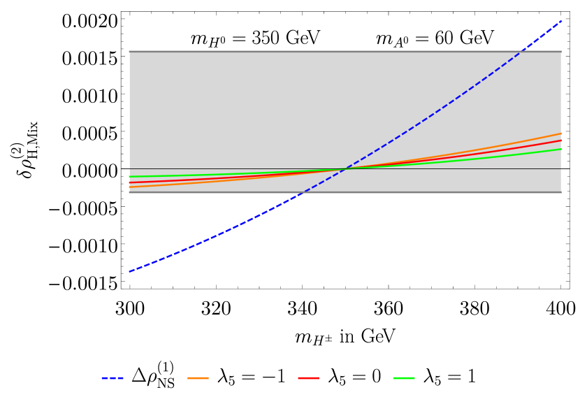
Figure 16: Results for $\delta\rho_{\text{H,Mix}}^{\text{(2)}}$ for $m_{A^{0}}=60\text{ GeV}$. The mass of $H^{0}$ is fixed at $350\text{ GeV}$. The different solid lines correspond to different values of $\lambda_{5}$, and the results are independent of $t_{\beta}$. The non-standard one-loop correction $\Delta\rho_{\text{NS}}^{\text{(1)}}$ is shown by the blue dashed line. The grey area corresponds to the bounds from the experimental limits of the $T$ parameter.

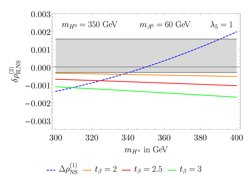
Figure 17: Results for $\delta\rho_{\text{H,NS}}^{\text{(2)}}$ for $m_{A^{0}}=60\text{ GeV}$. The mass of $H^{0}$ is fixed at $350\text{ GeV}$. The different solid lines correspond to different values of $t_{\beta}$. The non-standard one-loop correction $\Delta\rho_{\text{NS}}^{\text{(1)}}$ is shown by the blue dashed line. The grey area corresponds to the bounds from the experimental limits of the $T$ parameter.

8 Conclusions

We have given an overview over the calculation of the two-loop contributions to the $\rho$-parameter in the $CP$-conserving Two-Higgs-Doublet Model where one of the $CP$-even scalars ($h^{0}$) is identified with the scalar resonance at 125 GeV observed by the LHC experiments ATLAS and CMS. The approximation of the gauge-less limit and massless fermions except the top quark yield the leading contributions from the top-Yukawa coupling and the self-couplings of the Higgs bosons, which can be separated into standard and non-standard contributions. As already at the one-loop level, the non-standard contributions from the scalar self-interactions are particularly sensitive to mass splittings between neutral and charged scalars. As a new feature, the two-loop contributions have a significant dependence on the parameters $\tan\beta$ and $\lambda_{5}$, the coefficient of the THDM scalar potential that is not fixed by the masses of the neutral and charged Higgs bosons, and thus can modify the one-loop result substantially. Moreover, this significant dependence on the additional parameters can be exploited to get more indirect information on the Higgs potential from electroweak precision data than with the currently available one-loop calculations.

The loop correction $\Delta\rho$ to the $\rho$-parameter is an important entry in the calculation of electroweak precision observables, parametrizing dominant universal contributions from particles with mass splitting in isospin doublets, in the THDM in particular from neutral and charged Higgs bosons. For an estimate of the impact of a shift in $\Delta\rho$ on the prediction of the $W$ mass and the effective weak mixing angle $\sin^{2}\theta_{\rm eff}$ at $M_{Z}$, one can use the approximate expressions

$$\Delta M_{W}\simeq\frac{M_{W}}{2}\,\frac{c_{W}^{2}}{c_{W}^{2}-s_{W}^{2}}\,\Delta\rho,$$ (172)

$$\Delta\sin^{2}\theta_{\rm eff}\simeq-\frac{c_{W}^{2}s_{W}^{2}}{c_{W}^{2}-s_{W}^{2}}\,\Delta\rho,$$ (173)

to translate the two-loop contribution to $\Delta\rho$ from the non-standard Higgs sector obtained in this paper into shifts of the observables. An accurate evaluation of the precision observables and implications from comparisons with experimental data requires a more detailed study, which will be presented in a forthcoming publication.

Appendix A Feynman rules for the counterterm vertices

In the counterterm vertices in the diagrams in figure 2 and figure 3 we keep only the counterterms which survive the gauge-less limit. These are the mass counterterms of the top quark and the non-standard scalars and the renormalization constant $\delta s_{W}^{2}$ which has a remaining contribution in the gauge-less limit (see section 5). All field counterterms are dropped since they either cancel in the full result or vanish in the gauge-less limit. In the vertices all the momenta are considered as incoming. Dropping field renormalization, the scalar–scalar two-point vertex counterterm takes the form

$=-i\delta m_{S}^{2}$

for $S=h^{0},H^{0},A^{0},H^{\pm},G^{0},G^{\pm}$.

The Feynman rule involving the top-quark mass counterterm is given by

$=-i\delta m_{t}$.

The renormalization conditions for the mass counterterms are given in section 5.

For the coupling of a massive gauge boson to two scalars we obtain the following counterterm vertices:

$=\left(k_{1}-k_{2}\right)_{\mu}C\left[V_{\mu},S_{1},S_{2}\right]$

$$C[Z_{\mu},h^{0},G^{0}] =\frac{e}{4s_{W}c_{W}}\frac{\left(s_{W}^{2}-c_{W}^{2}\right)}{c_{W}^{2}}\frac{\delta s_{W}^{2}}{s_{W}^{2}},$$

$$C[Z_{\mu},H^{0},A^{0}] =-\frac{e}{4s_{W}c_{W}}\frac{\left(s_{W}^{2}-c_{W}^{2}\right)}{c_{W}^{2}}\frac{\delta s_{W}^{2}}{s_{W}^{2}},$$

$$C[Z_{\mu},H^{-},H^{+}] =-i\frac{e}{4s_{W}c_{W}^{3}}\frac{\delta s_{W}^{2}}{s_{W}^{2}},$$

$$C[Z_{\mu},G^{-},G^{+}] =-i\frac{e}{4s_{W}c_{W}^{3}}\frac{\delta s_{W}^{2}}{s_{W}^{2}},$$

$$C[W_{\mu}^{\pm},h^{0},G^{\mp}] =\pm i\frac{e}{4s_{W}}\frac{\delta s_{W}^{2}}{s_{W}^{2}},$$

$$C[W_{\mu}^{\pm},H^{0},H^{\mp}] =\mp i\frac{e}{4s_{W}}\frac{\delta s_{W}^{2}}{s_{W}^{2}},$$

$$C[W_{\mu}^{\pm},A^{0},H^{\mp}] =-\frac{e}{4s_{W}}\frac{\delta s_{W}^{2}}{s_{W}^{2}},$$

$$C[W_{\mu}^{\pm},G^{0},G^{\mp}] =-\frac{e}{4s_{W}}\frac{\delta s_{W}^{2}}{s_{W}^{2}},$$

For the coupling of two massive gauge bosons to two scalars the counterterm vertices are

$=g_{\mu\nu}C\left[V_{\mu},V_{\nu},S_{1},S_{2}\right]$

$$C[Z_{\mu},Z_{\nu},h^{0},h^{0}] =i\frac{e^{2}}{2s_{W}^{2}c_{W}^{2}}\frac{s_{W}^{2}-c_{W}^{2}}{c_{W}^{2}}\frac{\delta s_{W}^{2}}{s_{W}^{2}},$$

$$C[Z_{\mu},Z_{\nu},H^{0},H^{0}] =i\frac{e^{2}}{2s_{W}^{2}c_{W}^{2}}\frac{s_{W}^{2}-c_{W}^{2}}{c_{W}^{2}}\frac{\delta s_{W}^{2}}{s_{W}^{2}},$$

$$C[Z_{\mu},Z_{\nu},A^{0},A^{0}] =i\frac{e^{2}}{2s_{W}^{2}c_{W}^{2}}\frac{s_{W}^{2}-c_{W}^{2}}{c_{W}^{2}}\frac{\delta s_{W}^{2}}{s_{W}^{2}},$$

$$C[Z_{\mu},Z_{\nu},H^{+},H^{-}] =i\frac{e^{2}}{2s_{W}^{2}c_{W}^{2}}\frac{s_{W}^{2}-c_{W}^{2}}{c_{W}^{2}}\frac{\delta s_{W}^{2}}{s_{W}^{2}},$$

$$C[Z_{\mu},Z_{\nu},G^{0},G^{0}] =i\frac{e^{2}}{2s_{W}^{2}c_{W}^{2}}\frac{s_{W}^{2}-c_{W}^{2}}{c_{W}^{2}}\frac{\delta s_{W}^{2}}{s_{W}^{2}},$$

$$C[Z_{\mu},Z_{\nu},G^{+},G^{-}] =i\frac{e^{2}}{2s_{W}^{2}c_{W}^{2}}\frac{s_{W}^{2}-c_{W}^{2}}{c_{W}^{2}}\frac{\delta s_{W}^{2}}{s_{W}^{2}},$$

$$C[W_{\mu}^{+},W_{\nu}^{-},h^{0},h^{0}] =-i\frac{e^{2}}{2s_{W}^{2}}\frac{\delta s_{W}^{2}}{s_{W}^{2}},$$

$$C[W_{\mu}^{+},W_{\nu}^{-},H^{0},H^{0}] =-i\frac{e^{2}}{2s_{W}^{2}}\frac{\delta s_{W}^{2}}{s_{W}^{2}},$$

$$C[W_{\mu}^{+},W_{\nu}^{-},A^{0},A^{0}] =-i\frac{e^{2}}{2s_{W}^{2}}\frac{\delta s_{W}^{2}}{s_{W}^{2}},$$

$$C[W_{\mu}^{+},W_{\nu}^{-},H^{+},H^{-}] =-i\frac{e^{2}}{2s_{W}^{2}}\frac{\delta s_{W}^{2}}{s_{W}^{2}}.$$

$$C[W_{\mu}^{+},W_{\nu}^{-},G^{0},G^{0}] =-i\frac{e^{2}}{2s_{W}^{2}}\frac{\delta s_{W}^{2}}{s_{W}^{2}},$$

$$C[W_{\mu}^{+},W_{\nu}^{-},G^{+},G^{-}] =-i\frac{e^{2}}{2s_{W}^{2}}\frac{\delta s_{W}^{2}}{s_{W}^{2}},$$

The counterterm vertices between the gauge bosons and the fermions in figure 2 are given by

$=\left(C_{-}\omega_{-}+C_{+}\omega_{+}\right)\gamma_{\mu}$,

$$W^{+}\overline{t}b:\quad C_{+}=0,\quad C_{-}=i\frac{e}{2\sqrt{2}s_{W}}\frac{\delta s_{W}^{2}}{s_{W}^{2}},$$

$$W^{-}\overline{b}t:\quad C_{+}=0,\quad C_{-}=i\frac{e}{2\sqrt{2}s_{W}}\frac{\delta s_{W}^{2}}{s_{W}^{2}},$$

$$Z\overline{t}t:\quad C_{+}=i\frac{e}{3c_{W}^{2}}\frac{s_{W}}{c_{W}}\frac{\delta s_{W}^{2}}{s_{W}^{2}},\quad C_{-}=\frac{ie}{4c_{W}s_{W}}\left(1+\frac{1}{3}\frac{s_{W}^{2}}{c_{W}^{2}}\right)\frac{\delta s_{W}^{2}}{s_{W}^{2}}.$$

Appendix B One- and two-loop integrals

B.1 Scalar one-loop integrals

Here we list all the one- and two-loop scalar integrals that are used in our calculation. They are evaluated in dimensional regularization tHooft:1972fi ; Bollini:1972ui ; Ashmore:1972uj with dimension $D$ of the integrated momentum and the associated mass parameter $\mu_{D}$,

$$\int d^{4}q\rightarrow\mu^{4-D}_{D}\int d^{D}q\,.$$ (174)

The scalar integrals are expanded in $\delta=(D-4)/2$ and the divergencies appear as poles in $\delta$.

The reduction of the one-loop tensor integrals to scalar integrals and their classification is following the work of Passarino:1978jh ; tHooft:1978xw (for more details and notation see Denner:1991kt ). The only one-loop integrals which are needed for the evaluation of the self-energies are

$$A_{0}(m^{2})=\int\frac{d^{D}q}{i\pi^{2}}\frac{(2\pi\mu_{D})^{(4-D)}}{(q^{2}-m^{2}+i\epsilon)},$$ (175)

$$B_{0}(p^{2},m_{1}^{2},m_{2}^{2})\\ =\int\frac{d^{D}q}{i\pi^{2}}\frac{(2\pi\mu_{D})^{(4-D)}}{(q^{2}-m_{1}^{2}+i\epsilon)((p+q)^{2}-m_{2}^{2}+i\epsilon)}.$$ (176)

We need an expansion up to order $\delta$ of the scalar integrals; analytic expressions can be found in Nierste:1992wg ; Hollik:2014bua .

B.2 Scalar two-loop integrals

The notation of the two-loop integrals follows the conventions of Weiglein:1993hd . For vanishing external momentum all two-loop integrals in the self energies can be reduced to the scalar integral

$$T_{134}\left(m_{1}^{2},m_{2}^{2},m_{3}^{2}\right)=\left(\frac{(2\pi\mu_{D})^{(4-D)}}{i\pi^{2}}\right)^{2}\cdot\\ \int\frac{\text{d}^{D}q_{1}\text{d}^{D}q_{2}}{\left(k_{1}^{2}-m_{1}^{2}+i\epsilon\right)\left(k_{3}^{2}-m_{2}^{2}+i\epsilon\right)\left(k_{4}^{2}-m_{3}^{2}+i\epsilon\right)}$$ (177)

with $k_{1}=q_{1}$, $k_{3}=q_{2}-q_{1}$ and $k_{4}=q_{2}$.

This integral can be calculated analytically and the result can be found in Berends:1994ed ; Davydychev:1992mt .

References

- (1) G. Aad, et al., Phys.Lett. B716, 1 (2012). DOI 10.1016/j.physletb.2012.08.020
- (2) S. Chatrchyan, et al., Phys.Lett. B716, 30 (2012). DOI 10.1016/j.physletb.2012.08.021
- (3) G. Aad, et al., Phys. Rev. Lett. 114, 191803 (2015). DOI 10.1103/PhysRevLett.114.191803
- (4) G.C. Branco, P.M. Ferreira, L. Lavoura, M.N. Rebelo, M. Sher, J.P. Silva, Phys. Rept. 516, 1 (2012). DOI 10.1016/j.physrep.2012.02.002
- (5) S. Bertolini, Nucl. Phys. B272, 77 (1986). DOI 10.1016/0550-3213(86)90341-X
- (6) W. Hollik, Z. Phys. C32, 291 (1986). DOI 10.1007/BF01552507
- (7) W. Hollik, Z. Phys. C37, 569 (1988). DOI 10.1007/BF01549716
- (8) A. Denner, R.J. Guth, W. Hollik, J.H. Kühn, Z. Phys. C51, 695 (1991). DOI 10.1007/BF01565598
- (9) C.D. Froggatt, R.G. Moorhouse, I.G. Knowles, Phys. Rev. D45, 2471 (1992). DOI 10.1103/PhysRevD.45.2471
- (10) P.H. Chankowski, M. Krawczyk, J. Zochowski, Eur. Phys. J. C11, 661 (1999). DOI 10.1007/s100529900217,10.1007/s100520050662
- (11) W. Grimus, L. Lavoura, O.M. Ogreid, P. Osland, J. Phys. G35, 075001 (2008). DOI 10.1088/0954-3899/35/7/075001
- (12) W. Grimus, L. Lavoura, O.M. Ogreid, P. Osland, Nucl. Phys. B801, 81 (2008). DOI 10.1016/j.nuclphysb.2008.04.019
- (13) D. Lopez-Val, J. Sola, Eur. Phys. J. C73, 2393 (2013). DOI 10.1140/epjc/s10052-013-2393-y
- (14) R. Santos, A. Barroso, Phys. Rev. D56, 5366 (1997). DOI 10.1103/PhysRevD.56.5366
- (15) A. Arhrib, M. Capdequi Peyranere, W. Hollik, S. Penaranda, Phys. Lett. B579, 361 (2004). DOI 10.1016/j.physletb.2003.10.006
- (16) D. Lopez-Val, J. Sola, Phys. Rev. D81, 033003 (2010). DOI 10.1103/PhysRevD.81.033003
- (17) S. Kanemura, K. Tsumura, K. Yagyu, H. Yokoya, Phys. Rev. D90, 075001 (2014). DOI 10.1103/PhysRevD.90.075001
- (18) S. Kanemura, M. Kikuchi, K. Yagyu, Nucl. Phys. B896, 80 (2015). DOI 10.1016/j.nuclphysb.2015.04.015
- (19) M. Krause, R. Lorenz, M. Muhlleitner, R. Santos, H. Ziesche, JHEP 09, 143 (2016). DOI 10.1007/JHEP09(2016)143
- (20) A. Denner, L. Jenniches, J.N. Lang, C. Sturm, JHEP 09, 115 (2016). DOI 10.1007/JHEP09(2016)115
- (21) A. Djouadi, P. Gambino, S. Heinemeyer, W. Hollik, C. Jünger, G. Weiglein, Phys. Rev. Lett. 78, 3626 (1997). DOI 10.1103/PhysRevLett.78.3626
- (22) A. Djouadi, P. Gambino, S. Heinemeyer, W. Hollik, C. Jünger, G. Weiglein, Phys. Rev. D57, 4179 (1998). DOI 10.1103/PhysRevD.57.4179
- (23) S. Heinemeyer, G. Weiglein, JHEP 10, 072 (2002). DOI 10.1088/1126-6708/2002/10/072
- (24) J. Haestier, S. Heinemeyer, D. Stöckinger, G. Weiglein, JHEP 12, 027 (2005). DOI 10.1088/1126-6708/2005/12/027
- (25) J. F. Gunion, H. E. Haber, G. L. Kane and S. Dawson, The Higgs hunter’s guide (Perseus Publishing, Cambridge, Mass., 1990)
- (26) S.L. Glashow, S. Weinberg, Phys. Rev. D15, 1958 (1977). DOI 10.1103/PhysRevD.15.1958
- (27) E.A. Paschos, Phys. Rev. D15, 1966 (1977). DOI 10.1103/PhysRevD.15.1966
- (28) W.S. Hou, Phys. Lett. B296, 179 (1992). DOI 10.1016/0370-2693(92)90823-M
- (29) D. Chang, W.S. Hou, W.Y. Keung, Phys. Rev. D48, 217 (1993). DOI 10.1103/PhysRevD.48.217
- (30) D. Atwood, L. Reina, A. Soni, Phys. Rev. D55, 3156 (1997). DOI 10.1103/PhysRevD.55.3156
- (31) G. Aad, et al., Eur. Phys. J. C76(1), 6 (2016). DOI 10.1140/epjc/s10052-015-3769-y
- (32) V. Khachatryan, et al., Eur. Phys. J. C75(5), 212 (2015). DOI 10.1140/epjc/s10052-015-3351-7
- (33) P.S. Bhupal Dev, A. Pilaftsis, JHEP 12, 024 (2014). DOI 10.1007/JHEP11(2015)147,10.1007/JHEP12(2014)024. [Erratum: JHEP11,147(2015)]
- (34) J. Bernon, J.F. Gunion, H.E. Haber, Y. Jiang, S. Kraml, Phys. Rev. D92(7), 075004 (2015). DOI 10.1103/PhysRevD.92.075004
- (35) T. Hahn, Comput. Phys. Commun. 140, 418 (2001). DOI 10.1016/S0010-4655(01)00290-9
- (36) T. Hahn, M. Perez-Victoria, Comput. Phys. Commun. 118, 153 (1999). DOI 10.1016/S0010-4655(98)00173-8
- (37) G. Weiglein, R. Scharf, M. Böhm, Nucl. Phys. B416, 606 (1994). DOI 10.1016/0550-3213(94)90325-5
- (38) G. Weiglein, R. Mertig, R. Scharf, M. Böhm, in New computing techniques in physics research II. Proceedings, 2nd International Workshop on Software Engineering, Artificial Intelligence and Expert Systems in High-Energy and Nuclear Physics, La Londe les Maures, France, January 13-18, 1992, ed. by D. Perret-Gallix (1992), pp. 617–623
- (39) A.I. Davydychev, J.B. Tausk, Nucl. Phys. B397, 123 (1993). DOI 10.1016/0550-3213(93)90338-P
- (40) F.A. Berends, J.B. Tausk, Nucl. Phys. B421, 456 (1994). DOI 10.1016/0550-3213(94)90336-0
- (41) S. Heinemeyer, W. Hollik, G. Weiglein, Comput. Phys. Commun. 124, 76 (2000). DOI 10.1016/S0010-4655(99)00364-1
- (42) T. Hahn, S. Heinemeyer, W. Hollik, H. Rzehak, G. Weiglein, Comput. Phys. Commun. 180, 1426 (2009). DOI 10.1016/j.cpc.2009.02.014
- (43) T. Hahn, S. Paßehr, Implementation of the MSSM Higgs-mass corrections in (2015). ArXiv:1508.00562
- (44) S. Weinberg, Phys. Rev. D19, 1277 (1979). DOI 10.1103/PhysRevD.19.1277
- (45) L. Susskind, Phys. Rev. D20, 2619 (1979). DOI 10.1103/PhysRevD.20.2619
- (46) P. Sikivie, L. Susskind, M.B. Voloshin, V.I. Zakharov, Nucl. Phys. B173, 189 (1980). DOI 10.1016/0550-3213(80)90214-X
- (47) M.J.G. Veltman, Nucl. Phys. B123, 89 (1977). DOI 10.1016/0550-3213(77)90342-X
- (48) M.S. Chanowitz, M.A. Furman, I. Hinchliffe, Nucl. Phys. B153, 402 (1979). DOI 10.1016/0550-3213(79)90606-0
- (49) M.S. Chanowitz, M.A. Furman, I. Hinchliffe, Phys. Lett. B78, 285 (1978). DOI 10.1016/0370-2693(78)90024-2
- (50) S. Willenbrock, in Physics in . Proceedings, Theoretical Advanced Study Institute in elementary particle physics, TASI 2004, Boulder, USA, June 6-July 2, 2004 (2004), pp. 3–38
- (51) H.E. Haber, A. Pomarol, Phys.Lett. B302, 435 (1993). DOI 10.1016/0370-2693(93)90423-F
- (52) A. Pomarol, R. Vega, Nucl.Phys. B413, 3 (1994). DOI 10.1016/0550-3213(94)90611-4
- (53) J.M. Gerard, M. Herquet, Phys.Rev.Lett. 98, 251802 (2007). DOI 10.1103/PhysRevLett.98.251802
- (54) B. Grzadkowski, M. Maniatis, J. Wudka, JHEP 1111, 030 (2011). DOI 10.1007/JHEP11(2011)030
- (55) H.E. Haber, D. O’Neil, Phys.Rev. D83, 055017 (2011). DOI 10.1103/PhysRevD.83.055017
- (56) C. Nishi, Phys.Rev. D83, 095005 (2011). DOI 10.1103/PhysRevD.83.095005
- (57) F.J. Botella, J.P. Silva, Phys. Rev. D51, 3870 (1995). DOI 10.1103/PhysRevD.51.3870
- (58) S. Davidson, H.E. Haber, Phys. Rev. D72, 035004 (2005). DOI 10.1103/PhysRevD.72.099902,10.1103/PhysRevD.72.035004. [Erratum: Phys. Rev.D72,099902(2005)]
- (59) A. Denner, Fortsch.Phys. 41, 307 (1993)
- (60) D.A. Ross, M.J.G. Veltman, Nucl. Phys. B95, 135 (1975). DOI 10.1016/0550-3213(75)90485-X
- (61) R. Barbieri, M. Beccaria, P. Ciafaloni, G. Curci, A. Vicere, Nucl. Phys. B409, 105 (1993). DOI 10.1016/0550-3213(93)90448-X
- (62) J. Fleischer, O.V. Tarasov, F. Jegerlehner, Phys. Rev. D51, 3820 (1995). DOI 10.1103/PhysRevD.51.3820
- (63) M. Consoli, W. Hollik, F. Jegerlehner, Phys. Lett. B227, 167 (1989). DOI 10.1016/0370-2693(89)91301-4
- (64) J.J. van der Bij, F. Hoogeveen, Nucl. Phys. B283, 477 (1987). DOI 10.1016/0550-3213(87)90284-7
- (65) J. van der Bij, M.J.G. Veltman, Nucl. Phys. B231, 205 (1984). DOI 10.1016/0550-3213(84)90284-0
- (66) J. Fleischer, O.V. Tarasov, F. Jegerlehner, Phys. Lett. B319, 249 (1993). DOI 10.1016/0370-2693(93)90810-5
- (67) N.G. Deshpande, E. Ma, Phys. Rev. D18, 2574 (1978). DOI 10.1103/PhysRevD.18.2574
- (68) A. Arhrib, Y.L.S. Tsai, Q. Yuan, T.C. Yuan, JCAP 1406, 030 (2014). DOI 10.1088/1475-7516/2014/06/030
- (69) A. Arhrib, R. Benbrik, J. El Falaki, A. Jueid, JHEP 12, 007 (2015). DOI 10.1007/JHEP12(2015)007
- (70) C. Patrignani, et al., Chin. Phys. C40(10), 100001 (2016). DOI 10.1088/1674-1137/40/10/100001
- (71) M.E. Peskin, T. Takeuchi, Phys. Rev. Lett. 65, 964 (1990). DOI 10.1103/PhysRevLett.65.964
- (72) M.E. Peskin, T. Takeuchi, Phys. Rev. D46, 381 (1992). DOI 10.1103/PhysRevD.46.381
- (73) J.F. Gunion, H.E. Haber, Phys. Rev. D67, 075019 (2003). DOI 10.1103/PhysRevD.67.075019
- (74) A.G. Akeroyd, A. Arhrib, E.M. Naimi, Phys. Lett. B490, 119 (2000). DOI 10.1016/S0370-2693(00)00962-X
- (75) D. Das, Int. J. Mod. Phys. A30(26), 1550158 (2015). DOI 10.1142/S0217751X15501584
- (76) O. Deschamps, S. Descotes-Genon, S. Monteil, V. Niess, S. T’Jampens, V. Tisserand, Phys. Rev. D82, 073012 (2010). DOI 10.1103/PhysRevD.82.073012
- (77) T. Enomoto, R. Watanabe, JHEP 05, 002 (2016). DOI 10.1007/JHEP05(2016)002
- (78) J. Bernon, J.F. Gunion, Y. Jiang, S. Kraml, Phys. Rev. D91(7), 075019 (2015). DOI 10.1103/PhysRevD.91.075019
- (79) D. Chang, W.F. Chang, C.H. Chou, W.Y. Keung, Phys. Rev. D63, 091301 (2001). DOI 10.1103/PhysRevD.63.091301
- (80) A. Broggio, E.J. Chun, M. Passera, K.M. Patel, S.K. Vempati, JHEP 11, 058 (2014). DOI 10.1007/JHEP11(2014)058
- (81) E.J. Chun, J. Kim, JHEP 07, 110 (2016). DOI 10.1007/JHEP07(2016)110
- (82) G. ’t Hooft, M.J.G. Veltman, Nucl. Phys. B44, 189 (1972). DOI 10.1016/0550-3213(72)90279-9
- (83) C.G. Bollini, J.J. Giambiagi, Nuovo Cim. B12, 20 (1972). DOI 10.1007/BF02895558
- (84) J.F. Ashmore, Lett. Nuovo Cim. 4, 289 (1972). DOI 10.1007/BF02824407
- (85) G. Passarino, M.J.G. Veltman, Nucl. Phys. B160, 151 (1979). DOI 10.1016/0550-3213(79)90234-7
- (86) G. ’t Hooft, M.J.G. Veltman, Nucl. Phys. B153, 365 (1979). DOI 10.1016/0550-3213(79)90605-9
- (87) U. Nierste, D. Müller, M. Böhm, Z. Phys. C57, 605 (1993). DOI 10.1007/BF01561479
- (88) W. Hollik, S. Paßehr, JHEP 10, 171 (2014). DOI 10.1007/JHEP10(2014)171