Existence, Stability and Dynamics of Harmonically Trapped One-Dimensional Multi-Component Solitary Waves: The Near-Linear Limit

Abstract

In the present work, we consider a variety of two-component, one-dimensional states in nonlinear Schrödinger equations in the presence of a parabolic trap, inspired by the atomic physics context of Bose-Einstein condensates. The use of Lyapunov-Schmidt reduction methods allows us to identify persistence criteria for the different families of solutions which we classify as $(m,n)$, in accordance with the number of nodes in each component. Upon developing the existence theory, we turn to a stability analysis of the different configurations, using the Krein signature and the Hamiltonian-Krein index as topological tools identifying the number of potentially unstable eigendirections for each branch. A systematic expansion of suitably reduced eigenvalue problems when perturbing off of the linear limit permits us to obtain explicit expressions for the eigenvalues of each of the states considered. Finally, when the states are found to be unstable, typically by virtue of Hamiltonian Hopf bifurcations, their dynamics is studied in order to identify the nature of the respective instability. The dynamics is generally found to lead to a vibrational evolution over long time scales.

I Introduction

Models of the nonlinear Schrödinger (NLS) type sulem ; ablowitz ; siambook have proven to be rather universal in describing envelope nonlinear wave structures in dispersive media. Such structures emerge in fields ranging from water waves and nonlinear optics kivshar to plasmas infeld and atomic Bose-Einstein condensates (BECs) emergent . A particularly interesting setting, recognized early on (i.e., since the 1970’s) in nonlinear optics in the context of interaction of waves of different frequency is that of multi-component NLS models manakov . Among these, arguably, the most prototypical one is the integrable intman2 so-called Manakov model, which is characterized by equal nonlinear interactions within and across components.

Two decades after these initial developments within nonlinear optics, a renewed interest has emerged for such multi-component systems through the advent of ultra-cold atomic Bose-Einstein condensates (BECs) stringari ; roman . Numerous experiments since then have focused on realizing such multi-component BECs as mixtures of, e.g., different spin states of the same atom species (so-called pseudo-spinor condensates) Hall1998a ; chap01:stamp , or different Zeeman sub-levels of the same hyperfine level (spinor condensates) Stenger1998a ; kawueda ; stampueda . A remarkable feature of these atomic systems when they pertain to the same atomic species is that the so-called scattering lengths controlling the inter-atomic interactions and hence effectively the nonlinear prefactors are nearly equal within and across components both in settings of, e.g., ⁸⁷Rb and of ²³Na. This, in turn, translates in models well approximated by the Manakov nonlinearity, enabling the experimental realization not only of ground states, but also of numerous solitonic excitations, most notably of dark-bright solitons and their variants hamburg ; pe1 ; pe2 ; pe3 ; azu ; pe4 ; pe5 . These developments have been recently summarized in a number of reviews and books siambook ; emergent ; revip .

Our aim in the present work is to consider the harmonically trapped setting of atomic Bose-Einstein condensates in the context of the multi-component models discussed above. In earlier work, both a subset of the present authors todd1 ; todd2 , as well as other researchers feder explored the use of analytical techniques in order to examine the existence and stability of solutions in the vicinity of the well-understood linear (quantum harmonic oscillator) limit of single-component models featuring one atomic species. The relevant methods included, e.g., among others the use of Lyapunov-Schmidt conditions for persistence of solutions near this limit, as well as the use of the Krein signature and related topological index tools toddbook to characterize the stability of the resulting excitations. The topological tools are used to determine the potential number of unstable directions associated with an excitation, while the analysis allows us to determine which of the potential instabilities are realized.

Here, we extend such considerations to the more involved setting of two-component systems. While we will not do so in this paper, the ideas presented herein can be used to consider the existence and spectral stability of solutions to systems with three or more components. As in the one-component setting, nonlinear states emanate (bifurcate) from a corresponding linear state. In the one-component setting the linear state corresponds to an eigenfunction with a specified number of nodes which is associated with a simple eigenvalue. In the two-component case the eigenvalues are semi-simple, and in the cases considered herein will be of multiplicity two. At the linear level the first component will have $m$ nodes (i.e., we will denote the number of nodes of that component by $m$), while the second component will have $n$ nodes. The value of such topological and analytical tools in uncovering the potential number of unstable eigendirections of each such pair $(m,n)$ can be considerable in shaping the expectation of the potential experimental observability of different states.

It should be highlighted here that it does not escape us that low atom numbers are more prone to effects of quantum fluctuations potentially detrimental to the existence of the states (although it is our understanding that the study of such effects in multi-component systems is fairly limited). Nevertheless, our argument is that the value of considerations such as the topological ones presented herein is that they are of broader value in uncovering potential eigendirections beyond the vicinity of the linear limit and hence of relevance to regimes where the states could be observable as described by the mean-field Manakov-like limit discussed herein and as has been revealed experimentally e.g. in hamburg ; pe1 ; pe2 ; pe3 . For instance, an intriguing example of a finding that we present herein is that even the very robust (and experimentally identified) dark-bright soliton not only possesses a potentially unstable eigendirection, but this instability is realized provided that the inter-component interaction is increased sufficiently (an experimentally feasible scenario via the tuning of the inter-component scattering length by means of so-called Feshbach resonances siambook ).

Our presentation will be structured as follows. In section II, we will briefly present the theoretical setup and the analysis of the existence of the different solutions $(m,n)$. In section III, we will present a general framework for considering the stability of these states. In section IV, we catalogue the different possible states $(m,n)$ with $0\leq m,n\leq 2$. Finally, in section V we summarize our findings and present our conclusions, as well as a number of directions for future study.

II Theoretical setup and Existence Results

We consider the following two-component system, bearing in mind the setting of two hyperfine states of, e.g., ⁸⁷Rb revip

$$i\partial_{t}{\phi}_{1}(x,t) = (-\frac{1}{2}\partial_{xx}+\frac{1}{2}\Omega^{2}x^{2}-\mu_{1}){\phi}_{1}+(g_{11}|{\phi}_{1}|^{2}+g_{12}|\phi_{2}|^{2})\phi_{1},$$ (1)

$$i\partial_{t}\phi_{2}(x,t) = (-\frac{1}{2}\partial_{xx}+\frac{1}{2}\Omega^{2}x^{2}-\mu_{2})\phi_{2}+(g_{21}|\phi_{1}|^{2}+g_{22}|\phi_{2}|^{2})\phi_{2}$$ (2)

where $\phi_{j}\in\mathbb{C}$ is the mean-field wave-function of species $j,\,g_{jk}\in\mathbb{R}^{+}$ with $g_{12}=g_{21}$, $\mu_{j}\in\mathbb{R}$ represents the chemical potential for species $j$, and parabolic trapping potentials are considered here with the same trapping frequency $\Omega$ for both species; $\Omega$ effectively represents the ratio of the trapping strengths along the longitudinal (elongated) and transverse (strongly trapped) directions. Focusing on the wave functions such that $\int_{\mathbb{R}}|\phi_{j}(x)|^{2}dx=O(\epsilon)$ where $\epsilon\ll 1$ (i.e., the small amplitude, near-linear limit discussed in the previous section), we introduce the scaling $\phi_{j}=\epsilon^{1/2}\psi_{j}$ and obtain the following equations:

$$i\partial_{t}{\psi}_{1}(x,t) = f_{1}=(-\frac{1}{2}\partial_{xx}+\frac{1}{2}\Omega^{2}x^{2}-\mu_{1}){\psi}_{1}+\epsilon(g_{11}|{\psi}_{1}|^{2}+g_{12}|{\psi}_{2}|^{2}){\psi}_{1},$$ (3)

$$i\partial_{t}{\psi}_{2}(x,t) = f_{2}=(-\frac{1}{2}\partial_{xx}+\frac{1}{2}\Omega^{2}x^{2}-\mu_{2}){\psi}_{2}+\epsilon(g_{12}|{\psi}_{1}|^{2}+g_{22}|{\psi}_{2}|^{2}){\psi}_{2}$$ (4)

where $\int_{\mathbb{R}}|{\psi}_{j}(x)|^{2}dx=O(1)$ now. Due to the gauge invariance of the system, if $\{\psi_{1},\psi_{2}\}$ are a solution, then $\{\psi_{1}e^{i\theta_{1}},\psi_{2}e^{i\theta_{2}}\}$ will also be a solution for any real $\theta_{1}$ and $\theta_{2}$. In this paper we will focus on the existence and spectral stability of real-valued steady-state solutions for $\psi_{1}$ and $\psi_{2}$.

Set

$$\boldsymbol{\psi}=\left(\begin{array}[]{c}\psi_{1}\\ \psi_{2}\end{array}\right),\quad\boldsymbol{f}=\left(\begin{array}[]{c}f_{1}\\ f_{2}\end{array}\right),\quad\boldsymbol{\mu}=\left(\begin{array}[]{c}\mu_{1}\\ \mu_{2}\end{array}\right).$$

We seek the stationary solutions $\boldsymbol{\psi}(x,t)=\boldsymbol{\psi}(x)$ through the continuation of a nontrivial solution for $\epsilon=0$. For the moment assume the asymptotic expansions,

$$\boldsymbol{\psi}=\boldsymbol{\psi}^{(0)}+\epsilon\boldsymbol{\psi}^{(1)}+O(\epsilon^{2}),\,\,\boldsymbol{\mu}=\boldsymbol{\mu}^{(0)}+\epsilon\boldsymbol{\mu}^{(1)}+O(\epsilon^{2}).$$ (5)

These expansions will be verified through a Lyapunov-Schmidt reduction, which requires a detailed understanding of the linearized problem associated with (3)-(4) nirenberg . We linearize about the steady state solution by taking the Fréchet derivative of $\boldsymbol{f}({\boldsymbol{\psi}},{\boldsymbol{\psi}}^{*},\epsilon)$ and $\boldsymbol{f^{*}}({\boldsymbol{\psi}},{\boldsymbol{\psi}}^{*},\epsilon)$ with respect to ${\boldsymbol{\psi}}$ and ${\boldsymbol{\psi}}^{*}$; star here stands for complex conjugation. Let $\mathcal{L}$ denote the operator associated with the linearization having the asymptotic expansion $\mathcal{L}=\mathcal{L}^{0)}+\epsilon\mathcal{L}^{(1)}+O(\epsilon^{2})$, where

$$\mathcal{L}^{(0)}=\left(\begin{array}[]{cccc}-\frac{1}{2}\partial_{xx}+\frac{1}{2}\Omega^{2}x^{2}-\mu_{1}^{(0)}&0&0&0\\ 0&-\frac{1}{2}\partial_{xx}+\frac{1}{2}\Omega^{2}x^{2}-\mu_{1}^{(0)}&0&0\\ 0&0&-\frac{1}{2}\partial_{xx}+\frac{1}{2}\Omega^{2}x^{2}-\mu_{2}^{(0)}&0\\ 0&0&0&-\frac{1}{2}\partial_{xx}+\frac{1}{2}\Omega^{2}x^{2}-\mu_{2}^{(0)}\end{array}\right),$$ (10)

and

$$\begin{split}\mathcal{L}^{(1)}=\left(\begin{array}[]{cccc}2g_{11}|{\psi}_{1}^{(0)}|^{2}+g_{12}|{\psi}_{2}^{(0)}|^{2}&g_{11}({\psi}_{1}^{(0)})^{2}&g_{12}{\psi}_{1}^{(0)}{\psi}_{2}^{(0)}&g_{12}{\psi}_{1}^{(0)}{\psi}_{2}^{(0)}\\ g_{11}({\psi}_{1}^{(0)})^{2}&2g_{11}|{\psi}_{1}^{(0)}|^{2}+g_{12}|{\psi}_{2}^{(0)}|^{2}&g_{12}{\psi}_{1}^{(0)}{\psi}_{2}^{(0)}&g_{12}{\psi}_{1}^{(0)}{\psi}_{2}^{(0)}\\ g_{12}{\psi}_{1}^{(0)}{\psi}_{2}^{(0)}&g_{12}{\psi}_{1}^{(0)}{\psi}_{2}^{(0)}&2g_{22}|\psi_{2}^{(0)}|^{2}+g_{21}|\psi_{1}^{(0)}|^{2}&g_{22}({\psi}_{2}^{(0)})^{2}\\ g_{12}{\psi}_{1}^{(0)}{\psi}_{2}^{(0)}&g_{12}{\psi}_{1}^{(0)}{\psi}_{2}^{(0)}&g_{22}({\psi}_{2}^{(0)})^{2}&2g_{22}|{\psi}_{2}^{(0)}|^{2}+g_{21}|{\psi}_{1}^{(0)}|^{2}\end{array}\right).\end{split}$$ (11)

Focusing on real solutions, we can directly see a symmetry of $\mathcal{L}$:

$$J_{1}^{T}\mathcal{L}J_{1}=\mathcal{L},\quad J_{1}=\left(\begin{array}[]{cccc}0&1&0&0\\ 1&0&0&0\\ 0&0&0&1\\ 0&0&1&0\end{array}\right).$$ (12)

Using the linear eigenvalues of the quantum harmonic oscillator,

$$\mu_{1}^{(0)}=\Omega(m+\frac{1}{2}),\quad\mu_{2}^{(0)}=\Omega(n+\frac{1}{2}),$$

it can be directly observed that $\mathcal{L}^{(0)}$ has a non-empty kernel spanned by $\{(u_{m},0,0,0)^{T},(0,u_{m},0,0)^{T},(0,0,u_{n},0)^{T},(0,0,0,u_{n})^{T}\}$, where

$$u_{k}(x)=\sqrt{\frac{1}{2^{k}k!}}\left(\frac{\Omega}{\pi}\right)^{1/4}H_{k}(\sqrt{\Omega}x)e^{-\frac{\Omega x^{2}}{2}},$$

and $H_{k}$ are the Hermite polynomials. The first three states are

$$u_{0}(x)=\left(\frac{\Omega}{\pi}\right)^{1/4}e^{-\Omega x^{2}/2},\,\,u_{1}(x)=\left(\frac{\Omega}{\pi}\right)^{1/4}\sqrt{2\Omega}xe^{-\Omega x^{2}/2},\,\,u_{2}(x)=\left(\frac{\Omega}{\pi}\right)^{1/4}\sqrt{\frac{1}{2}}(2\Omega x^{2}-1)e^{-\Omega x^{2}/2}.$$

The collection of states $\{u_{0},u_{1},u_{2},\dots\}$ has the properties that:

1. $\displaystyle{\left(-\frac{1}{2}\partial_{xx}+\frac{1}{2}\Omega^{2}x^{2}\right)u_{j}=\Omega(j+\frac{1}{2})u_{j}}$ for each $j=0,1,2,\dots$

2. $u_{j}(x)$ has $j$ simple zeros for each $j=0,1,2,\dots$

3. the set is orthonormal under the inner product $\displaystyle{\langle g,h\rangle=\int_{\mathbb{R}}g(x)h(x)^{*}\,\mathrm{d}x}$

4. the set is a basis for $L^{2}(\mathbb{R})$.

We now consider the existence problem. We apply the Lyapunov-Schmidt Reduction Method to Eqs. (3)-(4) with

$$\boldsymbol{\mu}\approx\left(\begin{array}[]{c}\Omega(m+1/2)\\ \Omega(n+1/2)\end{array}\right).$$

The state will hereafter be denoted as $(m,n)$. Since the vector field is smooth, and the eigenvalues are semi-simple, the reduction guarantees that both $\boldsymbol{\mu}$ and $\boldsymbol{\psi}$ will have an asymptotic expansion in $\epsilon$ of (5). Equations (3)–(4) at order $O(1)$ are

$$0 = (-\frac{1}{2}\partial_{xx}+\frac{1}{2}\Omega^{2}x^{2}-\mu_{1}^{(0)}){\psi}_{1}^{(0)},$$ (13)

$$0 = (-\frac{1}{2}\partial_{xx}+\frac{1}{2}\Omega^{2}x^{2}-\mu_{2}^{(0)}){\psi}_{2}^{(0)}.$$ (14)

The nontrivial solution is the expected one,

$$\boldsymbol{\psi}^{(0)}=\left(\begin{array}[]{c}au_{m}\\ bu_{n}\end{array}\right),\quad\boldsymbol{\mu}^{(0)}=\left(\begin{array}[]{c}\Omega(m+1/2)\\ \Omega(n+1/2)\end{array}\right),$$

where $a,b\in\mathbb{R}$.

The next set of equations at $O(\epsilon)$ will provide the definitive values that $a$ and $b$ must assume. Equations (3)–(4) at order $O(\epsilon)$ are

$$0 = (-\frac{1}{2}\partial_{xx}+\frac{1}{2}\Omega^{2}x^{2}-\mu_{1}^{(0)}){\psi}_{1}^{(1)}+(g_{11}|{\psi}_{1}^{(0)}|^{2}+g_{12}|{\psi}_{2}^{(0)}|^{2}-\mu_{1}^{(1)}){\psi}_{1}^{(0)},$$ (15)

$$0 = (-\frac{1}{2}\partial_{xx}+\frac{1}{2}\Omega^{2}x^{2}-\mu_{2}^{(0)}){\psi}_{2}^{(1)}+(g_{12}|{\psi}_{1}^{(0)}|^{2}+g_{22}|{\psi}_{2}^{(0)}|^{2}-\mu_{2}^{(1)}){\psi}_{2}^{(0)}.$$ (16)

Solvability requires

$$0 = a(\mu_{1}^{(1)}-Ag_{11}a^{2}-Bg_{12}b^{2}),$$ (17)

$$0 = b(\mu_{2}^{(1)}-Bg_{12}a^{2}-Cg_{22}b^{2})$$ (18)

where

$$A=A_{m}=\langle u_{m}^{2},u_{m}^{2}\rangle,\quad B=B_{m,n}=\langle u_{m}^{2},u_{n}^{2}\rangle,\quad C=C_{n}=\langle u_{n}^{2},u_{n}^{2}\rangle.$$

Note that $A,B,C>0$ are positive real numbers; in particular, for a few values of the indices we have

$$A_{0}=C_{0}=B_{0,0}=\sqrt{\frac{\Omega}{2\pi}},\,\,A_{1}=C_{1}=B_{1,1}=\frac{3}{4}\sqrt{\frac{\Omega}{2\pi}},\,\,A_{2}=C_{2}=B_{2,2}=\frac{41}{64}\sqrt{\frac{\Omega}{2\pi}},$$

and

$$B_{1,0}=B_{0,1}=\frac{1}{2}\sqrt{\frac{\Omega}{2\pi}},\,\,B_{2,0}=B_{0,2}=\frac{3}{8}\sqrt{\frac{\Omega}{2\pi}},\,\,B_{2,1}=B_{1,2}=\frac{7}{16}\sqrt{\frac{\Omega}{2\pi}}.$$

Solving Eqs. (17)–(18) requires that for nontrivial solutions the pair $(a,b)$ should satisfy one of the following:

1. $a=0$, and $\displaystyle{b^{2}=\frac{\mu_{2}^{(1)}}{Cg_{22}}}$ for $\mu_{2}^{(1)}>0$

2. $b=0$, and $\displaystyle{a^{2}=\frac{\mu_{1}^{(1)}}{Ag_{11}}}$ for $\mu_{1}^{(1)}>0$

3. $a,b\neq 0$ and $\displaystyle{\left(\begin{array}[]{cc}Ag_{11}&Bg_{12}\\ Bg_{12}&Cg_{22}\end{array}\right)\left(\begin{array}[]{cc}a^{2}\\ b^{2}\end{array}\right)=\left(\begin{array}[]{cc}\mu_{1}^{(1)}\\ \mu_{2}^{(1)}\end{array}\right)}$.

Both the first and second case correspond to effectively single-component solutions, and will not be further considered in what follows except in a parenthetical manner. Regarding the third case,

$$ACg_{11}g_{22}-B^{2}g_{12}^{2}\neq 0\,\,\leadsto\,\,a^{2}=\frac{Cg_{22}\mu_{1}^{(1)}-Bg_{12}\mu_{2}^{(1)}}{ACg_{11}g_{22}-B^{2}g_{12}^{2}}>0,\quad b^{2}=\frac{Ag_{11}\mu_{2}^{(1)}-Bg_{12}\mu_{1}^{(1)}}{ACg_{11}g_{22}-B^{2}g_{12}^{2}}>0.$$

On the other hand, if the coefficients $g_{11},g_{12},g_{22}$ are special enough such that $A_{m}C_{n}g_{11}g_{22}-B_{m,n}^{2}g_{12}^{2}=0$ for some $(m,n)$, then the nontrivial two-component solutions for the state $(m,n)$ will exist only if

$$\frac{\mu_{1}^{(1)}}{\mu_{2}^{(1)}}=\frac{Ag_{11}}{Bg_{12}}.$$

Moreover, when those two-component solutions exist, $a$ and $b$ are not uniquely determined by $\mu_{1}^{(1)}$ and $\mu_{2}^{(1)}$ as in the above but there exists a family of available values for them. It is worthwhile to note that this condition is reminiscent of the phase separation criterion between two components and, in fact, coincides with the latter when $m=n$ siambook ; emergent . Nevertheless, we will not focus on this singular case here and in that light, in all that follows we focus on the cases where $ab\neq 0$ and $ACg_{11}g_{22}-B^{2}g_{12}^{2}\neq 0$, and without loss of generality assume $m\leq n$.

III Spectral stability

If $\boldsymbol{{\psi}}$ is a steady-state solution to the system (3)–(4), then we consider the perturbation ansatz ${\tilde{\psi}}_{j}(x,t)={\psi}_{j}+\delta(e^{\lambda t}v_{j}(x)+e^{\lambda^{*}t}w_{j}^{*}(x))$ of such a solution. After substituting $\boldsymbol{{\tilde{\psi}}}$ back into the system and linearizing around the solution $\boldsymbol{{\psi}}$, we obtain the eigenvalue problem,

$$J\mathcal{L}\boldsymbol{\xi}=i\lambda\boldsymbol{\xi}\quad\leadsto\quad(-iJ)\mathcal{L}\boldsymbol{\xi}=\lambda\boldsymbol{\xi},$$ (19)

where $J={\rm diag}(1,-1,1,-1)$ and $\boldsymbol{\xi}=(v_{1},w_{1},v_{2},w_{2})^{T}$. The operator $-iJ$ is skew-symmetric, and the operator $\mathcal{L}$ is self-adjoint. Consequently, this is a Hamiltonian eigenvalue problem. Because the solutions are purely real, an important consequence is that the eigenvalues satisfy the four-fold symmetry, $\{\pm\lambda,\pm\lambda^{*}\}$, which can also be explicitly seen from (12). Moreover, because of the unbounded potential term $\Omega^{2}x^{2}/2$ in the operator $\mathcal{L}$, the spectrum is purely discrete, and each eigenvalue has finite geometric and algebraic multiplicity.

III.1 The unperturbed spectrum

The spectrum for small $\epsilon$ will be determined via a perturbation expansion from the $\epsilon=0$ spectrum. Consequently, it is important to first have a detailed description of the unperturbed spectrum. For a given eigenvalue, $\lambda$, let $E_{\lambda}$ denote the corresponding eigenspace. It is straightforward to infer that given the quantum harmonic oscillator nature of its constituents, the eigenvalues of $(-iJ)\mathcal{L}^{(0)}$ are $-i\ell\Omega,\,\ell\in\mathbb{Z}$. Due to the four-fold spectral symmetry we can focus on the lower-half complex plane in the following. For each nonnegative $\ell$ there are three possibilities:

1. if $\ell\leq m$, then for $\lambda^{(0)}=-i\ell\Omega$,

   $$E_{-i\ell\Omega}=\mathrm{Span}\left\{\left(\begin{array}[]{c}u_{m+\ell}\\ 0\\ 0\\ 0\end{array}\right),\left(\begin{array}[]{c}0\\ u_{m-\ell}\\ 0\\ 0\end{array}\right),\left(\begin{array}[]{c}0\\ 0\\ u_{n+\ell}\\ 0\end{array}\right),\left(\begin{array}[]{c}0\\ 0\\ 0\\ u_{n-\ell}\end{array}\right)\right\}$$

2. if $m<\ell\leq n$, then for $\lambda^{(0)}=-i\ell\Omega$,

   $$E_{-i\ell\Omega}=\mathrm{Span}\left\{\left(\begin{array}[]{c}u_{m+\ell}\\ 0\\ 0\\ 0\end{array}\right),\left(\begin{array}[]{c}0\\ 0\\ u_{n+\ell}\\ 0\end{array}\right),\left(\begin{array}[]{c}0\\ 0\\ 0\\ u_{n-\ell}\end{array}\right)\right\}$$

3. If $\ell>n$, then for $\lambda^{(0)}=-i\ell\Omega$,

   $$E_{-i\ell\Omega}=\mathrm{Span}\left\{\left(\begin{array}[]{c}u_{m+\ell}\\ 0\\ 0\\ 0\end{array}\right),\left(\begin{array}[]{c}0\\ 0\\ u_{n+\ell}\\ 0\end{array}\right)\right\}.$$

The kernel has dimension four.

III.2 Krein Signature and Hamiltonian-Krein Index

The spectrum of $(-iJ)\mathcal{L}$ is completely known for the unperturbed problem. In particular, it is purely imaginary, so that the unperturbed wave is spectrally stable. Because of the four-fold symmetry, eigenvalues which are simple will remain purely imaginary for small $\epsilon$. However, as we see above the unperturbed eigenvalues are semi-simple, which implies that some could gain a nontrivial real part upon perturbation. Our first goal is to show via the Hamiltonian-Krein index (HKI) that all but a finite number of the eigenvalues will remain purely imaginary under small perturbation. Moreover, the index will precisely locate which among the infinitely many eigenvalues can gain nonzero real part under perturbation. See  toddbook for a more detailed exposition of what follows.

For the operator $(-iJ)\mathcal{L}$ let $k_{\mathrm{r}}$ denote the total number of real positive eigenvalues (counting multiplicity), and $k_{\mathrm{c}}$ the total number of eigenvalues with positive real part and nonzero imaginary part (counting multiplicity). Regarding the purely imaginary eigenvalues, let $\lambda$ be a purely imaginary eigenvalue with finite multiplicity, and let $E_{\lambda}$ denote the associated eigenspace. The negative Krein index associated with $E_{\lambda}$ is $k_{\mathrm{i}}^{-}(\lambda)=\mathrm{n}(\mathcal{L}|_{E_{\lambda}})$. Here $\mathrm{n}(S)$ denotes the number of negative eigenvalues (counting multiplicity) associated with a Hermitian matrix $S$, and $\mathcal{L}|_{E_{\lambda}}$ denotes the Hermitian matrix induced by restricting $\mathcal{L}$ to operate on $E_{\lambda}$. If $\lambda$ is a simple eigenvalue with associated eigenvector $\boldsymbol{\xi}$, then $\mathrm{n}(\mathcal{L}|_{E_{\lambda}})=\mathrm{n}(\langle\boldsymbol{\xi},\mathcal{L}\boldsymbol{\xi}\rangle)$. The eigenvalue is said to have positive Krein signature if $\mathrm{n}(\mathcal{L}|_{E_{\lambda}})=0$; otherwise, it is said to have negative Krein signature. Let $k_{\mathrm{i}}^{-}$ denote the total negative Krein index,

$$k_{\mathrm{i}}^{-}=\sum_{\lambda\in\sigma(-(iJ)\mathcal{L})\cap i\mathbb{R}}k_{\mathrm{i}}^{-}(\lambda).$$

The HKI is the sum of all three indices,

$$K_{\mathrm{Ham}}=k_{\mathrm{r}}+k_{\mathrm{c}}+k_{\mathrm{i}}^{-}.$$

Because of the four-fold eigenvalue symmetry, $k_{\mathrm{c}}$ and $k_{\mathrm{i}}^{-}$ will be even integers. In particular, there will be precisely $k_{\mathrm{c}}/2$ eigenvalues with positive real part and negative imaginary part, and $k_{\mathrm{i}}^{-}/2$ purely imaginary eigenvalues with negative imaginary part and negative Krein index.

The negative Krein index can be easily computed for the unperturbed problem. Again, we focus only on those eigenvalues with negative imaginary part. Using the diagonal form of $\mathcal{L}^{(0)}$, and the bases for the spectral subspaces given in the previous subsection, we find

1. if $\lambda=-i\ell\Omega$ with $0<\ell\leq m$, then $k_{\mathrm{i}}^{-}(-i\ell\Omega)=2$

2. if $\lambda=-i\ell\Omega$ with $m<\ell\leq n$, then $k_{\mathrm{i}}^{-}(-i\ell\Omega)=1$

3. if $\lambda=-i\ell\Omega$ with $n<\ell$, then $k_{\mathrm{i}}^{-}(-i\ell\Omega)=0$.

The four-fold symmetry implies that the eigenvalues with positive imaginary part satisfy $k_{i}^{-}(i\ell\Omega)=k_{i}^{-}(-i\ell\Omega)$ for any $l\in\mathbb{N}$. Consequently, the total negative Krein index is

$$k_{\mathrm{i}}^{-}=4m+2(n-m)=2(m+n),$$

so the HKI for the unperturbed problem is

$$K_{\mathrm{Ham}}=2(m+n).$$

Half of these eigenvalues have negative imaginary part, and half have positive imaginary part.

Since the index is integer-valued, for operators which depend continuously on parameters it remains unchanged for small perturbations. This statement, however, requires that no additional eigenvalues can be added into the mix via a bifurcation from the origin. Recall that we consider only those waves which are nontrivial in both components. The gauge symmetry implies that the geometric multiplicity of the origin will always be minimally two, and the Hamiltonian structure of the spectral problem means the algebraic multiplicity will always then be minimally four. For the unperturbed problem the algebraic multiplicity of the origin is precisely four. Since the origin is isolated, this then implies that for small perturbations the multiplicity will remain four. Consequently, we know that for small $\epsilon$,

$$K_{\mathrm{Ham}}=2(m+n),$$

and for those eigenvalues associated with the HKI having nonzero imaginary part, half will have positive imaginary part, and half will have negative imaginary part.

The HKI provides for an upper bound of the number of eigenvalues with positive real part. In order to locate those eigenvalues with small positive real part for the perturbed problem, we do a perturbation expansion. However, it is not necessary for us to perform an expansion for each eigenvalue. Purely imaginary eigenvalues can leave the imaginary axis only via the collision of eigenvalues of opposite Krein signature. This implies that for the perturbation expansion we only need to consider those eigenvalues for which the induced matrix $\mathcal{L}^{(0)}|_{E_{-i\ell\Omega}}$ is indefinite.

Restricting to those eigenvalues with negative imaginary part, this means we only have $\ell>0$. If $0<\ell\leq m$, the facts that $\mathrm{dim}[E_{-i\ell\Omega}]=4$ and $k_{\mathrm{i}}^{-}(-i\ell\Omega)=2$ imply that at most two eigenvalues can be created with positive real part (collision of a pair of eigenvalues with negative Krein signature with a pair with positive Krein signature). If $m<\ell\leq n$, the facts that $\mathrm{dim}[E_{-i\ell\Omega}]=3$ and $k_{\mathrm{i}}^{-}(-i\ell\Omega)=1$ imply that at most one eigenvalue can be created with positive real part (collision of one eigenvalue with negative Krein signature with one with positive Krein signature). Finally, if $\ell>n$ then the unperturbed eigenvalue has positive Krein signature, and will consequently remain purely imaginary under small perturbation. In conclusion, when performing the perturbation expansion we need only start with those unperturbed eigenvalues with $0<\ell\leq n$.

III.3 Reduced Eigenvalue Problem

Knowing the Hamiltonian-Krein index, we will examine the exact number of eigenvalue pairs with nonzero growth rates (i.e., associated with instabilities) by finding the leading-order correction to each eigenvalue. Since the eigenvalues are semi-simple, and the underlying solution is smooth in $\epsilon$, the eigenvalues and associated eigenfunctions have the expansions,

$$\lambda=\lambda^{(0)}+\epsilon\lambda^{(1)}+O(\epsilon^{2}),\quad\boldsymbol{\xi}=\boldsymbol{\xi}^{(0)}+\epsilon\boldsymbol{\xi}^{(1)}+O(\epsilon^{2}).$$

The $O(1)$ and $O(\epsilon)$ reductions of Eqn. (19) as

$$\left(\mathcal{L}^{(0)}-i\lambda^{(0)}J\right)\boldsymbol{\xi}^{(0)} = \boldsymbol{0}$$ (20)

$$\left(\mathcal{L}^{(0)}-i\lambda^{(0)}J\right)\boldsymbol{\xi}^{(1)} = \left(i\lambda^{(1)}J-\mathcal{L}^{(1)}\right)\boldsymbol{\xi}^{(0)}.$$ (21)

Letting $\{\boldsymbol{\eta}_{i}\}$ be an orthonormal basis for $E_{-i\ell\Omega}$, upon writing $\boldsymbol{\xi}^{(0)}=\sum c_{i}\boldsymbol{\eta}_{i}$ the solvability condition for (21) is the reduced spectral problem,

$$M\boldsymbol{c}=i\lambda^{(1)}\boldsymbol{c}.$$ (22)

Here

$$M_{j,k}=\langle\boldsymbol{\eta}_{j},J\mathcal{L}^{(1)}\boldsymbol{\eta}_{k}\rangle,$$

where the inner-product on each component is the standard one for $L^{2}(\mathbb{R})$. Similar calculations have been presented in different examples (chiefly for single component systems); see for one such example, e.g., todd3 . Note that if the spectrum of $M$ is purely real, then to leading order the eigenvalues will be purely imaginary. On the other hand, eigenvalues of $M$ which have nonzero imaginary part lead to an oscillatory instability for the underlying wave.

For the expansion we need only consider those eigenvalues with $\lambda^{(0)}=-i\ell\Omega$ for $0<\ell\leq n$. The perturbed eigenvalues for $\ell>n$ will remain purely imaginary. The size of the matrix $M$ will depend upon the value of $\ell$; in particular, if $0<\ell\leq m$, then $M\in\mathcal{M}_{4\times 4}(\mathbb{R})$, while if $m<\ell\leq n$, then $M\in\mathcal{M}_{3\times 3}(\mathbb{R})$. Defining

$$D_{p,q,r,s}:=\langle u_{p}u_{q},u_{r}u_{s}\rangle,$$

the explicit expression for $M$ is:

• $\lambda^{(0)}=-i\ell\Omega$ with $0<\ell\leq m$, then $M=M_{a}$, where

  $$M_{a}=\left(\begin{array}[]{cc}\tilde{M}_{11}&\tilde{M}_{12}\\ \tilde{M}_{21}&\tilde{M}_{22}\end{array}\right),$$

  and the individual blocks are defined via

  $$\tilde{M}_{11}=\left(\begin{array}[]{cc}2g_{11}a^{2}B_{m,m+\ell}+g_{12}b^{2}B_{n,m+\ell}-\mu_{1}^{(1)}&g_{11}a^{2}D_{m,m,m+\ell,m-\ell}\\ -g_{11}a^{2}D_{m,m,m+\ell,m-\ell}&-(2g_{11}a^{2}B_{m,m-\ell}+g_{12}b^{2}B_{n,m-\ell})+\mu_{1}^{(1)}\end{array}\right),$$

  and

  $$\tilde{M}_{12}=g_{12}ab\left(\begin{array}[]{cc}D_{m,n,m+\ell,n+\ell}&D_{m,n,m+\ell,n-\ell}\\ -D_{m,n,m-\ell,n+\ell}&-D_{m,n,m-\ell,n-\ell}\end{array}\right),\quad\tilde{M}_{21}=g_{12}ab\left(\begin{array}[]{cc}D_{m,n,m+\ell,n+\ell}&D_{m,n,m-\ell,n+\ell}\\ -D_{m,n,m+\ell,n-\ell}&-D_{m,n,m-\ell,n-\ell}\end{array}\right),$$

  and

  $$\tilde{M}_{22}=\left(\begin{array}[]{cc}2g_{22}b^{2}B_{n,n+\ell}+g_{12}a^{2}B_{m,n+\ell}-\mu_{2}^{(1)}&g_{22}b^{2}D_{n,n,n+\ell,n-\ell}\\ -g_{22}b^{2}D_{n,n,n+\ell,n-\ell}&-(2g_{22}b^{2}B_{n,n-\ell}+g_{12}a^{2}B_{m,n-\ell})+\mu_{2}^{(1)}\end{array}\right)$$

• If $\lambda^{(0)}=-i\ell\Omega$ where $m<\ell\leq n$, then $M=M_{b}$, and $M_{b}$ is simply the submatrix obtained from $M_{a}$ after removing the second row and second column.

Before continuing, we briefly comment on what the above perturbation calculation says about the spectral stability of one-component solutions. If $a=0$, then

$$\tilde{M}_{11}=\left(\begin{array}[]{cc}g_{12}b^{2}B_{m+\ell,n}-\mu_{1}^{(1)}&0\\ 0&-g_{12}b^{2}B_{m-\ell,n}+\mu_{1}^{(1)}\end{array}\right),\quad\tilde{M}_{22}=g_{22}b^{2}\left(\begin{array}[]{cc}2B_{n,n+\ell}-C&D_{n,n,n-\ell,n+\ell}\\ -D_{n,n,n-\ell,n+\ell}&C-2B_{n-\ell,n}\end{array}\right),$$

and $\tilde{M}_{12}=\tilde{M}_{21}=\boldsymbol{0}$. Thus, $M_{a}$ can have complex eigenvalues only if $|B_{n-\ell,n}+B_{n,n+\ell}-C|<|D_{n,n,n-\ell,n+\ell}|$. Similarly, when $b=0,\,M_{a}$ will have a complex spectrum only if $|B_{m-\ell,m}+B_{m,m+\ell}-A|<|D_{m,m,m-\ell,m+\ell}|$. When $a=0$, the condition for $M_{b}$ to have complex eigenvalues will be the same as that for $M_{a}$. If $b=0$, $M_{b}$ will simply become a diagonal matrix and always have a real spectrum.

Therefore, for a one-component solution where $(\psi_{1}^{(0)},\psi_{2}^{(0)})=(au_{m},0)$, its spectral stability can be examined by checking conditions $|B_{m-\ell,m}+B_{m,m+\ell}-A_{m}|<|D_{m,m,m-\ell,m+\ell}|$ for $0<\ell\leq m$. Here we note that this is the same stability result if we consider a single one-component equation. For $m\leq 2$ we can directly check the stability conditions for the one-component solutions to get:

1. if $m=0$, the solutions continued from $au_{0}$ are spectrally stable for small $\epsilon$;

2. if $m=1$, it can be checked that $|B_{0,1}+B_{1,2}-A_{1}|=|1/2+7/16-3/4|>|\sqrt{2}/8|=|D_{0,1,1,2}|$, so the solutions continued from $au_{1}$ are spectrally stable for small $\epsilon$;

3. if $m=2$, it can be checked that $|B_{1,2}+B_{2,3}-A_{2}|=|7/16+51/128-41/64|>|5\sqrt{6}/64|=|D_{1,2,2,3}|$ but $|B_{0,2}+B_{2,4}-A_{2}|=|3/8+329/1024-41/64|<|3\sqrt{6}/128|=|D_{0,2,2,4}|$, so the splitting of eigenvalues at $2\Omega$ will enter the complex plane and the solutions continued from $au_{2}$ are spectrally unstable (these stability features are well known, e.g., from the work of coles ).

In fact, in Section IV.7 we show that, in general,

$$\frac{|B_{m-1,m}+B_{m,m+1}-A_{m}|}{|D_{m,m,m-1,m+1}|}=\sqrt{\frac{m}{m+1}}+\sqrt{\frac{m+1}{m}}>2,\quad m\geq 1.$$

That is to say, the eigenvalues for one-component solutions near $-i\Omega$ will always stay on the imaginary axis, although this perturbation calculation itself doesn’t rule out the possibility for other eigenvalues to enter the complex plane.

IV Catalogue of Different $(m,n)$ Cases

We now use the theory of the previous section to compute the spectral stability of various two-component solutions. In particular, we will assume $0\leq m\leq n\leq 2$. In what follows, the different branches are presented for $\Omega=0.1$, although similar results have been obtained for other values of $\Omega$. In fact, the value of $\Omega$ does not have a significant bearing on the agreement between analytical predictions and computational results (including in the more physically realistic case of $\Omega\ll 1$).

IV.1 $(m,n)=(0,0)$

For $\mu_{1}^{(0)}=\mu_{2}^{(0)}=\Omega/2$, we consider the branches of solutions continued from $({\psi}_{1}^{(0)},{\psi}_{2}^{(0)})=(au_{0},bu_{0})$, where

$$a^{2}=\sqrt{\frac{2\pi}{\Omega}}\,\frac{g_{22}\mu_{1}^{(1)}-g_{12}\mu_{2}^{(1)}}{g_{11}g_{22}-g_{12}^{2}},\quad b^{2}=\sqrt{\frac{2\pi}{\Omega}}\,\frac{g_{11}\mu_{2}^{(1)}-g_{12}\mu_{1}^{(1)}}{g_{11}g_{22}-g_{12}^{2}}.$$

This state features the fundamental (ground state) waveform in both components of the system. Since $K_{\mathrm{Ham}}=0$ when $\epsilon=0$, the wave is spectrally (indeed, orbitally) stable for small $\epsilon$, and it is not necessary to perform the perturbation calculation.

IV.2 $(m,n)=(0,1)$ (interchange all subscripts to obtain case $(1,0)$)

If $\mu_{1}^{(0)}=\Omega/2$ and $\mu_{2}^{(0)}=3\Omega/2$, we consider the continuation of $({\psi}_{1}^{(0)},{\psi}_{2}^{(0)})=(au_{0},bu_{1})$, where

$$a^{2}=\sqrt{\frac{2\pi}{\Omega}}\,\frac{3g_{22}\mu_{1}^{(1)}-2g_{12}\mu_{2}^{(1)}}{3g_{11}g_{22}-g_{12}^{2}},\quad b^{2}=2\sqrt{\frac{2\pi}{\Omega}}\,\frac{2g_{11}\mu_{2}^{(1)}-g_{12}\mu_{1}^{(1)}}{3g_{11}g_{22}-g_{12}^{2}},$$

which corresponds to a “dark-bright” configuration. This configuration has been extensively studied in experiments over the past decade, as has been recently summarized e.g. in revip .

Regarding the spectral stability we have $K_{\mathrm{Ham}}=2$, with the dangerous eigenvalues at $\lambda^{(0)}=\pm i\Omega$. At most one eigenvalue with positive real part will emerge from $-i\Omega$. For the perturbation calculation we only need consider case (b), where $M_{b}\in\mathcal{M}_{3\times 3}(\mathbb{R})$ is

$$M_{b}=\frac{1}{8}\sqrt{\frac{\Omega}{2\pi}}\left(\begin{array}[]{ccc}2g_{12}b^{2}&\sqrt{2}g_{12}ab&4g_{12}ab\\ \sqrt{2}g_{12}ab&g_{22}b^{2}-g_{12}a^{2}&\sqrt{2}g_{22}b^{2}\\ -4g_{12}ab&-\sqrt{2}g_{22}b^{2}&-2g_{22}b^{2}-4g_{12}a^{2}\end{array}\right).$$ (23)

Regarding the spectrum of $M_{b}$, we have the following proposition:

Proposition IV.1.

$M_{b}$ for $(m,n)=(0,1)$ (i.e. the matrix in (23)) has an eigenvalue zero with associated eigenvector $(-a/b,-\sqrt{2},1)^{\mathrm{T}}$, and two other eigenvalues

$$-\frac{1}{16}\sqrt{\frac{\Omega}{2\pi}}\left(5a^{2}g_{12}-2b^{2}g_{12}+b^{2}g_{22}\pm\sqrt{9a^{4}g_{12}^{2}+18a^{2}b^{2}g_{12}(g_{22}-2g_{12})+b^{4}(2g_{12}+g_{22})^{2}}\right).$$

The eigenvalues of $M_{b}$ will have nonzero imaginary parts if and only if $g_{12}>g_{22}$.

The presence of the zero eigenvalue is well-known to be associated with the invariance of the condensate to dipolar oscillations with the frequency of the trap $\Omega$, yielding the so-called Kohn mode in the spectrum with the trap frequency (and hence vanishing perturbations off of the linear limit) stringari . This proposition can be verified via direct calculation and in Section IV.7 we will state more general results. It is intriguing that the expression for the nonzero eigenvalues for $M_{b}$ here does not include $g_{11}$. This is due to the fact that $A_{0}-2B_{0,1}=0$. As stated in Proposition IV.1, $M_{b}$ will have eigenvalues with nonzero imaginary parts –leading to an instability– if $g_{12}>g_{22}$, i.e., the inter-component interactions have to be stronger than the interactions within the “dark” species.

As an example, when $a=b=1$ the growth rate is

$$|\mathrm{Re}(\lambda^{(1)})|=\frac{1}{16}\sqrt{\frac{\Omega}{2\pi}(23g_{12}+g_{22})(g_{12}-g_{22})}\,I_{g_{12}>g_{22}}(g_{12}),$$

where

$$I_{g_{12}>g_{22}}(g_{12})=\begin{cases}0,\quad&g_{12}\leq g_{22}\\ 1,\quad&g_{12}>g_{22}.\end{cases}$$

In Figure 1, a case associated with this potential instability scenario of the $(0,1)$ branch is shown. In particular, the maximal real part of numerically computed eigenvalues from Eqn. (19) is plotted with respected to $g_{12}$ and $\epsilon$. We see that the numerical result is in good agreement with with our prediction $\epsilon|\mathrm{Re}(\lambda^{(1)})|$. It is relevant to indicate that in the integrable limit of $g_{ij}=1$, this instability does not manifest itself, but it should be observable in systems away from this limit provided that the first excited (dark) state is initialized in the “wrong” component i.e., the one with intra-component interactions $g_{22}<g_{12}$, while the fundamental state is initialized in the component with $g_{11}$.

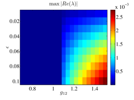
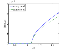
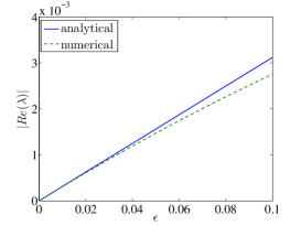
Figure 1: Stability features of the $(0,1)$ branch: in the left panel, we set $g_{22}=1.06,a=b=1$ and plot the maximal real part of numerically computed eigenvalues as a function of $g_{12}$ and $\epsilon$. In the middle (right) panel, we fix $\epsilon=0.1$ ($g_{12}=1.5$) for the setups in the left panel and compare the numerical result with analytical prediction $\epsilon|\mathrm{Re}(\lambda^{(1)})|$, as a function of $g_{12}$ ($\epsilon$). We find very good agreement in the dependence of the relevant eigenvalue.

In Fig. 2, we present the example with $a=b=1,g_{11}=1.03,g_{12}=1.04,g_{22}=1.06,\Omega=0.1$, comparing eigenvalue predictions with corrections up to $O(\epsilon)$ with corresponding numerical results. We find that all of the eigenvalues in the numerical computation are on the imaginary axis, which matches our analytical prediction. According to our numerical computation, the spectrum will remain purely imaginary even when $\epsilon$ is large, which is shown in the left panel of Fig. 3. In addition, we find that $\phi_{2}$ becomes $0$ at $\epsilon\approx 2.6$ where the branch of solutions meets the branch of single-component solutions on $\phi_{1}$.

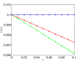
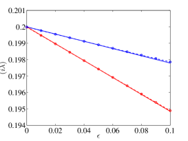
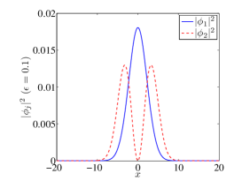
Figure 2: The left (middle) panel shows the imaginary parts of the eigenvalues around $-i\Omega$ ($-i2\Omega$) as functions of $\epsilon$ with $O(\epsilon)$ corrections (solid lines) and corresponding numerical results (dashed lines with circles) in the case of $(m,n)=(0,1)$, i.e., a prototypical example of a dark state with $n=1$ coupled to a fundamental state of $m=0$. In the right panel, we show the densities of $\phi_{1}$ and $\phi_{2}$ at $\epsilon=0.1$.

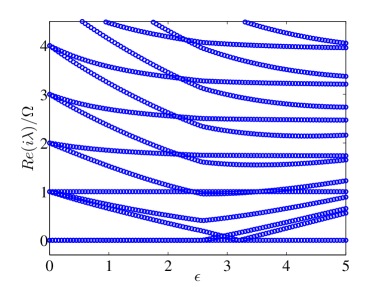
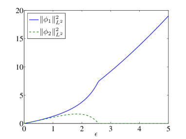
Figure 3: In the left panel, we plot the imaginary parts of the eigenvalues over a wide interval of parametric variation of $\epsilon$. The right panel shows the $L^{2}$-norm of the corresponding solution of $\phi_{1}$ and $\phi_{2}$ for such interval of $\epsilon$.

As another example, we consider a case that is “immediately unstable” in the vicinity of the linear limit. In particular, if $a=b=1,g_{11}=1.03,g_{12}=1.2,g_{22}=1.06,\Omega=0.1$, the numerical computation shows that all of the eigenvalues except a quartet (near $\pm i\Omega$) are purely imaginary, as shown in Fig. 4. As $\epsilon$ increases, we notice that the quartet will finally come back to the real axis at $\epsilon\approx 0.7$ and split along it, which is shown in Figure 5.

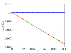
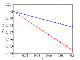
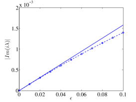
Figure 4: The left (middle) panel shows the imaginary parts of the eigenvalues around $-i\Omega$ ($-i2\Omega$) as functions of $\epsilon$ with $O(\epsilon)$ corrections (solid lines) and corresponding numerical results (dashed lines with circles). In the left panel, the red lines and green lines (solid and dashed) are identical since a pair of eigenvalues of $M_{b}$ for $\lambda^{(0)}=-i\Omega$ are complex conjugates. Moreover, the nonzero imaginary parts of $i\lambda$ for this pair imply the instability (this is the only source of the instability) of the solution, as shown in the right panel (solid line for the $O(\epsilon)$ correction using this pair of complex conjugates and the dashed line for the numerical computation of the real parts of the relevant eigenvalues).

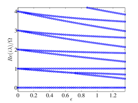
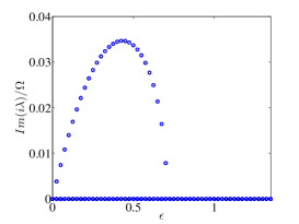
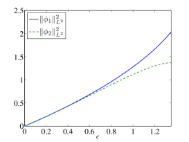
Figure 5: The left (middle) panel shows the variation of the imaginary (real) parts of the eigenvalues for the branch of solutions with $a=b=1$, $g_{11}=1.03$, $g_{12}=1.2$, $g_{22}=1.06$, $\Omega=0.5$. In the right panel, we plot the $L^{2}$-norm of the solution of $\phi_{j}$ over the same interval of $\epsilon$.

Figure 6 illustrates the numerical evolution of the unstable configuration shown in Figure 4 with $\epsilon=0.1$. If a small initial perturbation is added to the solution, the development of the instability can be observed over intermediate time scales in Figure 6. To determine the fate of the solution under the action of this instability, we have performed considerably longer simulations focusing on the dynamics of the unstable waveform (see the middle panels of Figure 6). There we find an oscillatory pattern of the long-term dynamics of the solution, featuring breathing (yet not genuinely periodic) recurrences over time. To be more specific, the bottom panels in Figure 6 reveal, through a dynamical decomposition to the lowest order harmonic oscillator modes, that the system does not stay at a certain state but quantitatively alternates between the states $(0,1)$ and $(1,0)$. We also observe that the instability of the state $(0,1)$ (similar for the state $(1,0)$) is essentially caused by the eigenmodes that are related to the unstable eigenvalues near $\pm i\Omega$, which is verified by the fact that both the time evolution of $|c_{1}|$ for $\phi_{1}$ and that of $|c_{0}|$ for $\phi_{2}$ bear small oscillations whose frequency is close to $\frac{2\pi}{\Omega}$.

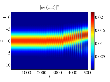
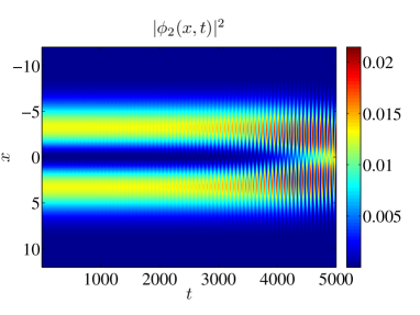
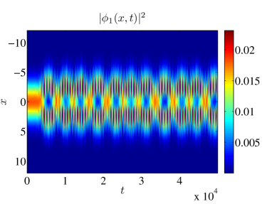
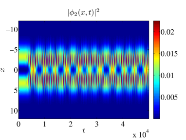
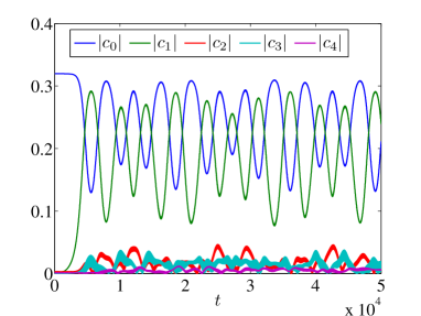
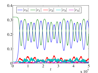
Figure 6: The top left (right) panel illustrates an example of the dynamics of $|\phi_{1}|^{2}$ ($|\phi_{2}|^{2}$) with $a=b=1$, $g_{11}=1.03$, $g_{12}=1.2$, $g_{22}=1.06$, $\Omega=0.1$ and $\epsilon=0.1$ for the $(0,1)$ state. The middle panels show the dynamics for the same setup for a longer time, revealing its oscillatory nature, while the bottom panels (left for $\phi_{1}$ and right for $\phi_{2}$) show the dynamics upon decomposition to the orthonormal basis $\{u_{k}\}$, where the diagnostic $c_{k}$ used stands for the coefficient (i.e., prefactor) of $u_{k}$ in the decomposition.

IV.3 $(m,n)=(1,1)$

When $\mu_{1}^{(0)}=\mu_{2}^{(0)}=3\Omega/2$, we consider $({\psi}_{1}^{(0)},{\psi}_{2}^{(0)})=(au_{1},bu_{1})$, where

$$a^{2}=\frac{4}{3}\sqrt{\frac{2\pi}{\Omega}}\,\frac{g_{22}\mu_{1}^{(1)}-g_{12}\mu_{2}^{(1)}}{g_{11}g_{22}-g_{12}^{2}},\quad b^{2}=\frac{4}{3}\sqrt{\frac{2\pi}{\Omega}}\,\frac{g_{11}\mu_{2}^{(1)}-g_{12}\mu_{1}^{(1)}}{g_{11}g_{22}-g_{12}^{2}}.$$

This state corresponds to a (co-located) dark-dark type configuration featuring a first excited state in both components. Regarding the spectral stability we have $K_{\mathrm{Ham}}=4$, with the dangerous eigenvalues again at $\lambda^{(0)}=\pm i\Omega$. At most two eigenvalues with positive real part will emerge from $-i\Omega$. For the perturbation calculation we need to consider case (a), where $M_{a}\in\mathcal{M}_{4\times 4}(\mathbb{R})$ is

$$M_{a}=\frac{1}{16}\sqrt{\frac{\Omega}{2\pi}}\left(\begin{array}[]{cccc}2g_{11}a^{2}-5g_{12}b^{2}&2\sqrt{2}g_{11}a^{2}&7g_{12}ab&2\sqrt{2}g_{12}ab\\ -2\sqrt{2}g_{11}a^{2}&-4g_{11}a^{2}+4g_{12}b^{2}&-2\sqrt{2}g_{12}ab&-8g_{12}ab\\ 7g_{12}ab&2\sqrt{2}g_{12}ab&2g_{22}b^{2}-5g_{12}a^{2}&2\sqrt{2}g_{22}b^{2}\\ -2\sqrt{2}g_{12}ab&-8g_{12}ab&-2\sqrt{2}g_{22}b^{2}&-4g_{22}b^{2}+4g_{12}a^{2}\end{array}\right).$$

Examining the spectrum of $M_{a}$, we find that one eigenvalue is zero with associated eigenvector $(-\sqrt{2}\,a/b,a/b,-\sqrt{2},1)^{\mathrm{T}}$; once again, this is associated with the invariance to dipolar oscillations with the frap frequency. Since the matrix is real-valued, this then implies that there is at most one pair of eigenvalues with nonzero imaginary part. This is an important conclusion that is particular to the case of the parabolic trap: the presence of the well-known symmetry associated with the dipolar oscillations stringari does not allow in this case the broader spectrum of two potentially unstable eigendirections to lead to instabilities; instead, only such instability direction may be realized in practice.

For a particular example, if we fix $a=b=1$ and $g_{11}=g_{22}=1$, then the remaining three eigenvalues of $M_{a}$ are

$$\sqrt{\frac{\Omega}{2\pi}}\,\frac{1+g_{12}}{8},\quad\sqrt{\frac{\Omega}{2\pi}}\,\frac{-1\pm\sqrt{1-56g_{12}+136g_{12}^{2}}}{16}$$

Under these specific parameter values, there is one pair of eigenvalues that can enter the complex plane for

$$g_{12}\in\left(\frac{14-9\sqrt{2}}{68},\frac{14+9\sqrt{2}}{68}\right)\approx(0.0187,0.3931).$$

Again, setting $a=b=1,g_{11}=1.03,g_{12}=1.04,g_{22}=1.06,\Omega=0.1$ we compare some predicted eigenvalues up to $O(\epsilon)$ with corresponding numerical eigenvalues in Fig. 7. All of the numerically computed eigenvalues from Eqn. (19) for this example are imaginary, which matches the analytical result of the reduced spectral eigenvalue problem from Eqn. (22). As $\epsilon$ becomes large, we see a pair of eigenvalues enter the complex plane near $\pm i\Omega$ at $\epsilon\approx 4.9$ when the eigenvalue from $i\Omega$ collides with the eigenvalue from $3i\Omega$ (see Figure 8). We also note that this complex pair will come back to the imaginary axis at $\epsilon\approx 5.2$, i.e., the parametric interval of instability is fairly narrow in this case.

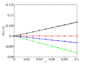
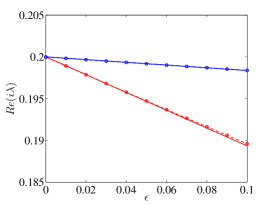
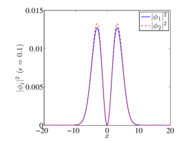
Figure 7: Case of $a=b=1,g_{11}=1.03,g_{12}=1.04,g_{22}=1.06,\Omega=0.1$ for the $(1,1)$ branch: The left (middle) panel shows the imaginary parts of the eigenvalues around $-i\Omega$ ($-2i\Omega$) as functions of $\epsilon$ with $O(\epsilon)$ corrections (solid lines) and corresponding numerical results (dashed lines with circles). The right panel shows the densities of $\phi_{1}$ and $\phi_{2}$ at $\epsilon=0.1$.

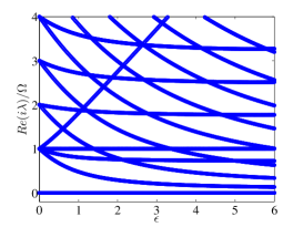
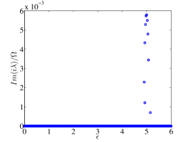
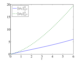
Figure 8: The left (middle) panel shows the change of imaginary (real) parts of the eigenvalues for the branch of solutions with $a=b=1,g_{11}=1.03,g_{12}=1.04,g_{22}=1.06,\Omega=0.1$ for the $(1,1)$ branch. In the right panel, we plot the $L^{2}$-norm of the solution of $\phi_{j}$ as a function of $\epsilon$.

If $a=b=1,g_{11}=1,g_{12}=0.25,g_{22}=1,\Omega=0.1$, the numerical computation shows that all of the eigenvalues except a quartet (near $\pm i\Omega$) are on the imaginary axis, as shown in Fig. 9. As $\epsilon$ grows, the complex pair of eigenvalues from $-i\Omega$ will return to the real axis and split into two, as seen in Figure 10. The split eigenvalue going upward will meet with the eigenvalue coming down from $-i3\Omega$ and produce another pair (quartet) of complex eigenvalues, which will go back to the imaginary axis and split again. One of the split eigenvalue will move upward and collide with the eigenvalue from $-i5\Omega$, which will again lead to complex eigenvalues, and so on. In Figure 11, we illustrate the numerical evolution of this unstable configuration for $\epsilon=0.1$. It can be seen that the weak (and clearly discerned to be oscillatory) nature of the instability only allows it to manifest over fairly long time scales, resulting in breathing dynamics.

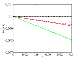
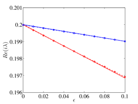
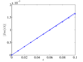
Figure 9: Case of the $(1,1)$ branch with $a=b=1,g_{11}=1,g_{12}=0.25,g_{22}=1,\Omega=0.1$: The left (middle) panel shows the imaginary parts of the eigenvalues around $-i\Omega$ ($-i2\Omega$) as functions of $\epsilon$ with $O(\epsilon)$ corrections (solid lines) and corresponding numerical results (dashed lines with circles). In the left panel, the red lines and blue lines (solid and dashed) are almost identical since a pair of eigenvalues of $M_{a}$ for $\lambda^{(0)}=-i\Omega$ are complex conjugates. Moreover, the nonzero imaginary parts of this pair imply the instability (this is the only source of the instability) of the solution, as shown in the right panel (solid line for the $O(\epsilon)$ correction using this pair of complex conjugates and the dashed line for the numerical computation of the real parts of the eigenvalues).

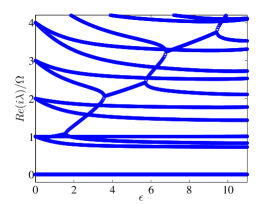
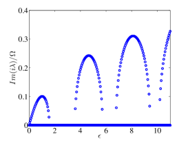
Figure 10: The left (middle) panel shows the change of imaginary (real) parts of the eigenvalues for the $(1,1)$ branch of solutions with $a=b=1,g_{11}=1,g_{12}=0.25,g_{22}=1,\Omega=0.1$. This is for a lengthy parametric continuation over $\epsilon$, featuring not only the original instability near the linear limit but subsequent splits (stabilizations) and further collisions (destabilizations) of the relevant solution. Again the right panel shows the $L^{2}$-norm of the solution of $\phi_{j}$ as a function of $\epsilon$.

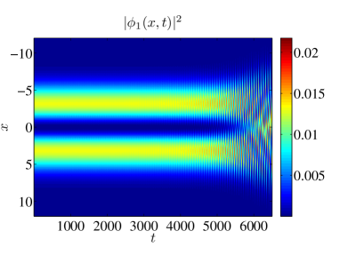
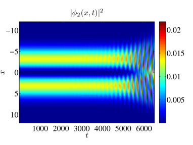
Figure 11: The left (right) panel shows an example of the dynamics of $|\phi_{1}|^{2}$ ($|\phi_{2}|^{2}$) of the $(1,1)$ branch with $a=b=1,g_{11}=1,g_{12}=0.25,g_{22}=1$, $\Omega=0.1$ and $\epsilon=0.1$.

IV.4 $(m,n)=(0,2)$

For $\mu_{1}^{(0)}=\Omega/2$ and $\mu_{2}^{(0)}=5\Omega/2$, we consider the continuation of $({\psi}_{1}^{(0)},{\psi}_{2}^{(0)})=(au_{0},bu_{2})$, where

$$a^{2}=64\sqrt{\frac{2\pi}{\Omega}}\,\frac{41g_{22}\mu_{1}^{(1)}-24g_{12}\mu_{2}^{(1)}}{41g_{11}g_{22}-9g_{12}^{2}},\quad b^{2}=512\sqrt{\frac{2\pi}{\Omega}}\,\frac{8g_{11}\mu_{2}^{(1)}-3g_{12}\mu_{1}^{(1)}}{41g_{11}g_{22}-9g_{12}^{2}}.$$

Regarding spectral stability we have $K_{\mathrm{Ham}}=4$, except that now the dangerous eigenvalues are at $\lambda^{(0)}=\pm i\Omega,\pm i2\Omega$. At most one eigenvalue with positive real part will emerge from each of these dangerous eigenvalues.

First consider the perturbation calculation associated with $\lambda^{(0)}=-i\Omega$. We consider case (b), and the matrix $M_{b}\in\mathcal{M}_{3\times 3}(\mathbb{R})$ is

$$M_{b}=\frac{1}{64}\sqrt{\frac{\Omega}{2\pi}}\left(\begin{array}[]{ccc}4g_{12}b^{2}&4\sqrt{3}\,g_{12}ab&8\sqrt{2}\,g_{12}ab\\ 4\sqrt{3}\,g_{12}ab&10g_{22}b^{2}-4g_{12}a^{2}&5\sqrt{6}\,g_{22}b^{2}\\ -8\sqrt{2}\,g_{12}ab&-5\sqrt{6}\,g_{22}b^{2}&-15g_{22}b^{2}-8g_{12}a^{2}\end{array}\right).$$ (24)

Proposition IV.2.

For $(m,n)=(0,2)$, the eigenvalues of $M_{b}$ in (24) are $0$ and

$$-\frac{1}{128}\sqrt{\frac{\Omega}{2\pi}}\left(12a^{2}g_{12}-4b^{2}g_{12}+5b^{2}g_{22}\pm\sqrt{16a^{4}g_{12}^{2}-8a^{2}b^{2}g_{12}(28g_{12}-25g_{22})+b^{4}(4g_{12}+5g_{22})^{2}}\right).$$

The imaginary parts of the eigenvalues for (24) will be nonzero if $g_{12}>5g_{22}/4$.

As is the case for the continuation of $(0,1)$, the parameter $g_{11}$ does not appear in the expressions of the eigenvalues.

Now consider the perturbation calculation associated with $\lambda^{(0)}=-i2\Omega$. In this case, the matrix $M_{b}\in\mathcal{M}_{3\times 3}(\mathbb{R})$ is

$$M_{b}=\frac{1}{512}\sqrt{\frac{\Omega}{2\pi}}\left(\begin{array}[]{ccc}-128g_{11}a^{2}+136g_{12}b^{2}&12\sqrt{6}g_{12}ab&192g_{12}ab\\ 12\sqrt{6}\,g_{12}ab&g_{22}b^{2}-52g_{12}a^{2}&12\sqrt{6}\,g_{22}b^{2}\\ -192g_{12}ab&-12\sqrt{6}\,g_{22}b^{2}&-56g_{22}b^{2}-320g_{12}a^{2}\end{array}\right).$$

Unfortunately, the expressions of eigenvalues are not as straightforward/enlightening in an analytical form (although available). As the numerical computations below show, it is possible for this matrix to have a pair of eigenvalues with nonzero imaginary part.

For the numerical computations, we again let $a=b=1,g_{11}=1.03,g_{12}=1.04,g_{22}=1.06,\Omega=0.1$, and compute the continuation of two-component solutions. We compare our analytical predictions providing the eigenvalues up to $O(\epsilon)$ with the corresponding numerical eigenvalues in Fig. 12. As $\epsilon$ grows, all of the numerically computed eigenvalues are on the imaginary axis and their change with respect to $\epsilon$ is illustrated in the left panel of Fig. 13. Additionally, we find that $\phi_{2}$ becomes zero at $\epsilon\approx 3.2$ where this branch of solutions meets the branch of one-component solutions on $\phi_{1}$. We note that this resembles the first example of case (0,1) very much.

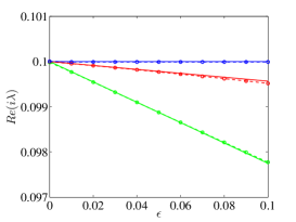
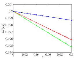
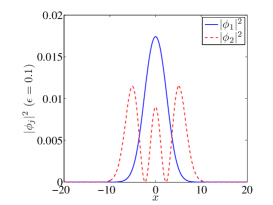
Figure 12: Case of the $(0,2)$ branch with $a=b=1,g_{11}=1.03,g_{12}=1.04,g_{22}=1.06,\Omega=0.1$: The left (middle) panel shows the imaginary parts of the eigenvalues around $-i\Omega$ ($-i2\Omega$) as functions of $\epsilon$ with $O(\epsilon)$ corrections (solid lines) and corresponding numerical results (dashed lines with circles). The right panel shows the densities of $\phi_{1}$ and $\phi_{2}$ at $\epsilon=0.1$ for this $(0,2)$ waveform.

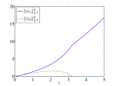
Figure 13: In the left panel, we keep track of the imaginary parts of the eigenvalues for large $\epsilon$ where the imaginary parts remain zero. The right panel shows the $L^{2}$-norm of the solution of $\phi_{j}$ for such variation of $\epsilon$.

However, in this case too, we can explore realistic scenarios where the instability manifests itself immediately in the vicinity of the linear limit. In particular, if $a=b=1,g_{11}=1,g_{12}=1,g_{22}=0.5,\Omega=0.1$, the numerical computation shows that there exist two quartets of eigenvalues (near $\pm i\Omega$ and $\pm i2\Omega$) that do not lie on the imaginary axis, as shown in Fig. 14. I.e., in this case, both unstable eigendirections of the system are realized and, in fact, potentially concurrently (contrary, e.g., to the case of $(1,1)$ waves). As $\epsilon$ grows, we observe that the complex pairs near $-i\Omega$ and $-i2\Omega$ tend to come back to the imaginary axis and split along the axis, as shown in Fig. 15. We observe that $\phi_{2}$ vanishes at $\epsilon\approx 0.8$ where the branch of solutions meets the one-component branch of solutions on $\phi_{1}$ there. In Figure 16, the numerically-monitored dynamics of the steady-state solution with a small initial perturbation verifies its instability. Here too, the instability manifests its oscillatory character and weak growth rate over longer time scales. In particular, the middle and bottom panels of Figure 16 show that the system first quantitatively alternates between unstable states $(0,2)$ and $(2,0)$ and then transits to the states that are close to $(0,1)$ and $(1,0)$. It can be checked that the dynamics of $|c_{2}|$ and $|c_{0}|$ comes with small oscillations with frequency close to $\frac{2\pi}{2\Omega}$, which implies that the instability in the first phase is related to the unstable eigenvalues near $\pm 2i\Omega$. Similarly, the time evolution of $|c_{1}|$ oscillates at the frequency of approximately $\frac{2\pi}{\Omega}$, which is connected to the unstable eigenvalues near $\pm i\Omega$. We note that the two-phase time evolution shown in Figure 16 is typical for our setup.

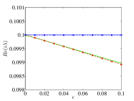
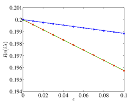
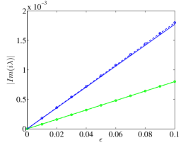
Figure 14: Case of $a=b=1,g_{11}=1,g_{12}=1,g_{22}=0.5,\Omega=0.1$ for the $(0,2)$ branch: The left (middle) panel shows the imaginary parts of $\lambda$’s around $\Omega$ ($2\Omega$) as functions of $\epsilon$ with $O(\epsilon)$ corrections (solid lines) and corresponding numerical results (dashed lines with circles). In these two panels, the red lines and green lines (solid and dashed) are almost identical since both $M_{b}$ for $\lambda^{(0)}=-i\Omega$ and $M_{b}$ for $\lambda^{(0)}=-i2\Omega$ have a pair of eigenvalues that are complex conjugates. Moreover, the nonzero imaginary parts of these pairs imply the instability of the solution, as shown in the right panel (solid lines for the $O(\epsilon)$ corrections using these pairs of complex conjugates and the dashed lines for the numerical computation of the real parts of the eigenvalues, blue for the ones near $-i\Omega$ and green for the ones near $-i2\Omega$).

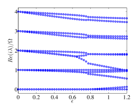
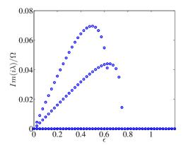
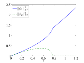
Figure 15: The left (middle) panel shows the change of imaginary (real) parts of $i\lambda$ for the branch of solutions with $a=b=1,g_{11}=1,g_{12}=1,g_{22}=0.5,\Omega=0.1$. The presence of the two associated instabilities is evident in the middle panel. In the right panel, we monitor the change of the $L^{2}$-norm of the solution of $\phi_{j}$ over $\epsilon$.

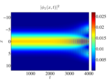
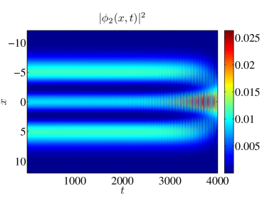
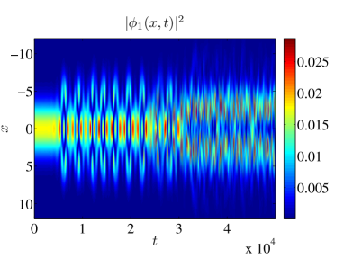
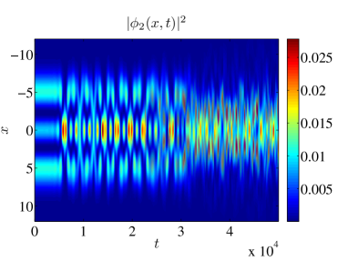
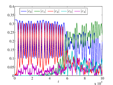
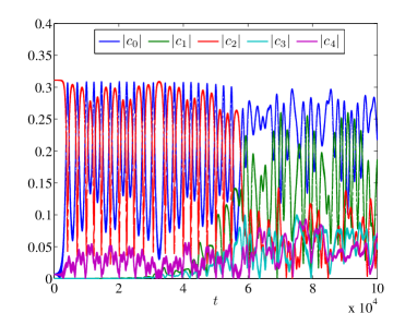
Figure 16: The top left (right) panel shows an example of the dynamics of $|\phi_{1}|^{2}$ ($|\phi_{2}|^{2}$) for the $(0,2)$ branch with $a=b=1,g_{11}=1,g_{12}=1,g_{22}=0.5$, $\Omega=0.1$ and $\epsilon=0.1$. In the middle panels, we monitor the dynamics of the same solution for a longer time, revealing the two stage nature of the evolution of the instability (see the relevant discussion in the text). The bottom panels show the same dynamics (left for $\phi_{1}$ and right for $\phi_{2}$) using the dynamical decomposition to the orthonormal basis $\{u_{k}\}$, where $c_{k}$ stands for the coefficient for $u_{k}$ in the decomposition. The transition between modes $(0,2)$ and $(2,0)$ originally to $(0,1)$ and $(1,0)$ eventually is evident in the mode dynamics.

IV.5 $(m,n)=(1,2)$ (interchange all subscripts to obtain $(m,n)=(2,1)$)

For $\mu_{1}^{(0)}=3\Omega/2$ and $\mu_{2}^{(0)}=5\Omega/2$ we consider the continuation of $({\psi}_{1}^{(0)},{\psi}_{2}^{(0)})=(au_{1},bu_{2})$, where

$$a^{2}=4\sqrt{\frac{2\pi}{\Omega}}\,\frac{41g_{22}\mu_{1}^{(1)}-28g_{12}\mu_{2}^{(1)}}{123g_{11}g_{22}-49g_{12}^{2}},\quad b^{2}=16\sqrt{\frac{2\pi}{\Omega}}\,\frac{12g_{11}\mu_{2}^{(1)}-7g_{12}\mu_{1}^{(1)}}{123g_{11}g_{22}-49g_{12}^{2}}.$$

Regarding spectral stability we have $K_{\mathrm{Ham}}=6$, and the dangerous eigenvalues are $\lambda^{(0)}=\pm i\Omega,\pm i2\Omega$. It is possible for a pair of eigenvalues with nonzero real part to emerge from $\pm i\Omega$, while at most one eigenvalue with positive real part can emerge from $\pm i2\Omega$.

First consider the perturbation calculation with $\lambda^{(0)}=-i\Omega$. We consider case (a), and $M_{a}\in\mathcal{M}_{4\times 4}(\mathbb{R})$ is

$$M_{a}=\frac{1}{64}\sqrt{\frac{\Omega}{2\pi}}\left(\begin{array}[]{cccc}8g_{11}a^{2}+13g_{12}b^{2}&8\sqrt{2}\,g_{11}a^{2}&5\sqrt{6}\,g_{12}ab&28g_{12}ab\\ -8\sqrt{2}\,g_{11}a^{2}&-16g_{11}a^{2}+4g_{12}b^{2}&-4\sqrt{3}\,g_{12}ab&-8\sqrt{2}\,g_{12}ab\\ 5\sqrt{6}\,g_{12}ab&4\sqrt{3}\,g_{12}ab&10g_{22}b^{2}-6g_{12}a^{2}&5\sqrt{6}\,g_{22}b^{2}\\ -28g_{12}ab&-8\sqrt{2}\,g_{12}ab&-5\sqrt{6}\,g_{22}b^{2}&-15g_{22}b^{2}-20g_{12}a^{2}\end{array}\right).$$

As per the dipolar mode that we discussed previously, one eigenvalue of $M_{a}$ is zero, with associated eigenvector $(-a/b,-a/(\sqrt{2}\,b,-\sqrt{6}/2,1)^{\mathrm{T}}$. Consequently, $M_{a}$ can have at most one pair of eigenvalues with nonzero imaginary part, which implies that at most one pair of eigenvalues with nonzero real part can emerge under the perturbation. If we particularly set $g_{11}=g_{22}=1$ and $a=b=1$, numerical results suggest a pair of complex conjugate eigenvalues will arise for $g_{12}>1$, as illustrated in the example below.

Now we consider the perturbation calculation with $\lambda^{(0)}=-i2\Omega$. We consider case (b), and $M_{b}\in\mathcal{M}_{3\times 3}(\mathbb{R})$ is

$$\frac{1}{512}\sqrt{\frac{\Omega}{2\pi}}\left(\begin{array}[]{ccc}-32g_{11}a^{2}-20g_{12}b^{2}&46\sqrt{2}\,g_{12}ab&32\sqrt{3}\,g_{12}ab\\ 46\sqrt{2}\,g_{12}ab&g_{22}b^{2}-74g_{12}a^{2}&12\sqrt{6}\,g_{22}b^{2}\\ -32\sqrt{3}\,g_{12}ab&-12\sqrt{6}\,g_{22}b^{2}&-56g_{22}b^{2}-32g_{12}a^{2}\end{array}\right).$$

This matrix can have at most one pair of eigenvalues with nonzero imaginary part, an example of which can be obtained for $g_{11}=g_{22}=1$, $a=b=1$ and $g_{12}>0$ (see Fig. 17).

For the numerical calculations we let $a=b=1,g_{11}=1,g_{12}=1.2,g_{22}=1,\Omega=0.1$ and we compare our analytical predictions for the leading order corrections to the eigenvalues up to $O(\epsilon)$ against the corresponding numerical eigenvalues in Fig. 17. We find two eigenvalue pairs (one pair each near $\pm i\Omega$ and $\pm i2\Omega$) introducing respective instability eigendirections. In Fig. 18, we see that the pairs near $-i\Omega$ and $-i2\Omega$ will eventually return to the imaginary axis, over considerably wider parametric continuations in $\epsilon$, splitting along the axis. Among these returned imaginary eigenvalues, the one that stems from $-i2\Omega$ and goes upward will meet the eigenvalue coming from $-i4\Omega$ to generate another pair of complex eigenvalues at $\epsilon\approx 2.7$. Shortly after (parametrically), these complex eigenvalues will come back to the axis and split into two eigenvalue pairs, with one of them going up to further repeat this process at $\epsilon\approx 3.6$ and $\epsilon\approx 4.2$.

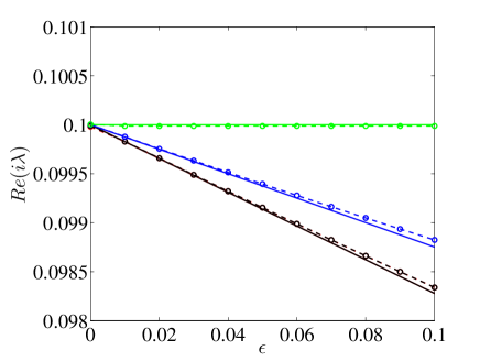
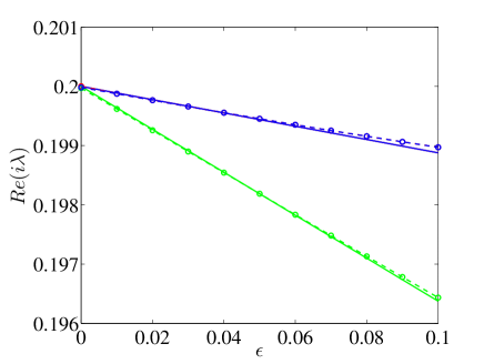
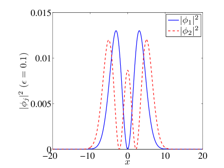
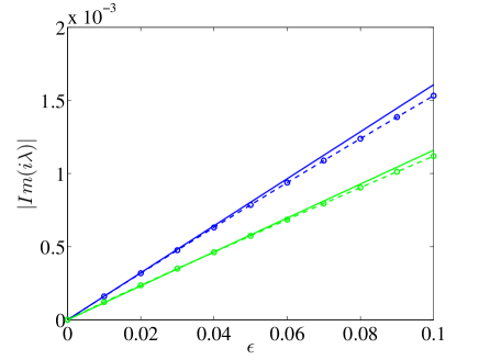
Figure 17: Case of $a=b=1,g_{11}=1,g_{12}=1.2,g_{22}=1,\Omega=0.1$ for the $(1,2)$ branch: The top left panel shows the real parts of $i\lambda$ around $\Omega$ as functions of $\epsilon$ with $O(\epsilon)$ corrections (solid lines) and corresponding numerical results (dashed lines with circles). The top right panel shows the real parts of $i\lambda$ around $2\Omega$. In both panels, it should be noticed that the red lines and green lines (solid and dashed) are almost identical since a pair of eigenvalues of $M_{a}$ and $M_{b}$ are complex conjugates. Moreover, the nonzero imaginary parts of these two pairs imply the instability of the solution, as shown in the bottom right panel (the growth rates are shown as solid lines for the predicted $O(\epsilon)$ corrections and as dashed lines for the numerical computation of the real parts of the eigenvalues; green for $M_{b}$ with $\lambda^{(0)}=-i2\Omega$ and blue for $M_{a}$ with $\lambda^{(0)}=-i\Omega$). The densities of $\phi_{1}$ and $\phi_{2}$ at $\epsilon=0.1$ are given in the bottom left panel.

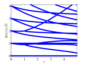
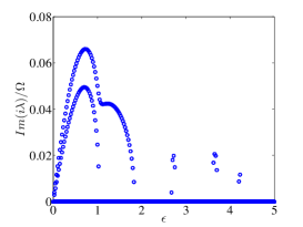
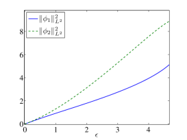
Figure 18: The left (middle) panel shows the change of imaginary (real) parts of the eigenvalues for the $(1,2)$ branch of solutions with $a=b=1,g_{11}=1,g_{12}=1.2,g_{22}=1,\Omega=0.1$. In this extended parametric continuation, the signature of the instabilities is evident in the middle panel of the figure. The right panel shows the change of the $L^{2}$-norm of the solution of $\phi_{j}$ over $\epsilon$.

In Figure 19, we illustrate the numerical evolution of the unstable configuration shown in Figure 17 with $\epsilon=0.1$. With a small initial perturbation, the oscillation around the stationary solution gradually grows and the instability becomes apparent in the dynamics.

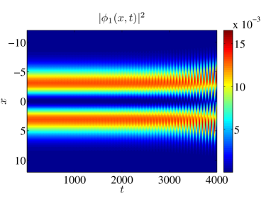
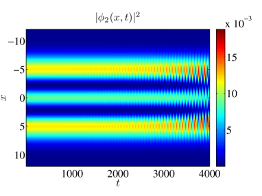
Figure 19: The left (right) panel shows an example of the dynamics of $|\phi_{1}|^{2}$ ($|\phi_{2}|^{2}$) for the $(1,2)$ state with $a=b=1,g_{11}=1,g_{12}=1.2,g_{22}=1$, $\Omega=0.1$ and $\epsilon=0.1$. Again, the oscillatory nature of the associated instability eventually kicks in over longer time scales.

IV.6 $(m,n)=(2,2)$

When $\mu_{1}^{(0)}=\mu_{2}^{(0)}=5\Omega/2$ we consider $({\psi}_{1}^{(0)},{\psi}_{2}^{(0)})=(au_{2},bu_{2})$, where

$$a^{2}=\frac{64}{\sqrt{41}}\sqrt{\frac{2\pi}{\Omega}}\,\frac{g_{22}\mu_{1}^{(1)}-g_{12}\mu_{2}^{(1)}}{g_{11}g_{22}-g_{12}^{2}},\quad b^{2}=\frac{64}{\sqrt{41}}\sqrt{\frac{2\pi}{\Omega}}\,\frac{g_{11}\mu_{2}^{(1)}-g_{12}\mu_{1}^{(1)}}{g_{11}g_{22}-g_{12}^{2}}.$$

Regarding spectral stability we have $K_{\mathrm{Ham}}=8$, and the dangerous eigenvalues are $\lambda^{(0)}=\pm i\Omega,\pm i2\Omega$. It is possible for two pairs of eigenvalues with nonzero real part to emerge from each of the dangerous eigenvalues.

First consider the perturbation calculation associated with $\lambda^{(0)}=-i\Omega$. We have case (a), and the matrix $M_{a}$ is

$$M_{a}=\frac{1}{128}\sqrt{\frac{\Omega}{2\pi}}\left(\begin{array}[]{cccc}20g_{11}a^{2}-31g_{12}b^{2}&10\sqrt{6}\,g_{11}a^{2}&51g_{12}ab&10\sqrt{6}\,g_{12}ab\\ -10\sqrt{6}\,g_{11}a^{2}&-30g_{11}a^{2}+26g_{12}b^{2}&-10\sqrt{6}\,g_{12}ab&-56g_{12}ab\\ 51g_{12}ab&10\sqrt{6}\,g_{12}ab&20g_{22}b^{2}-31g_{12}a^{2}&10\sqrt{6}\,g_{22}b^{2}\\ -10\sqrt{6}\,g_{12}ab&-56g_{12}ab&-10\sqrt{6}\,g_{22}b^{2}&-30g_{22}b^{2}+26g_{12}a^{2}\end{array}\right).$$

One of the eigenvalues is zero, with associated eigenvector $(-\sqrt{6}a/(2b),a/b,-\sqrt{6}/2,1)^{\mathrm{T}}$, for the same (dipolar) symmetry reasons as before. Consequently, $M_{a}$ can have at most one pair of eigenvalues with nonzero imaginary part, so at most one pair of eigenvalues with nonzero real part can emerge from $\pm i\Omega$. As an example, if we assume $a=b=1$ and $g_{11}=g_{22}=1$, then the other eigenvalues of $M_{a}$ are

$$-\frac{5}{64}\sqrt{\frac{\Omega}{2\pi}}\,(1+g_{12}),\quad\sqrt{\frac{\Omega}{2\pi}}\,\frac{-5\pm\sqrt{25-2900g_{12}+6124g_{12}^{2}}}{128}$$

where the instability (nonzero imaginary parts) will emerge for

$$g_{12}\in(\frac{725-285\sqrt{6}}{3062},\frac{725+285\sqrt{6}}{3062})\approx(0.0088,0.4648).$$

Now consider the perturbation calculation associated with $\lambda^{(0)}=-i2\Omega$. We again have case (a), and the matrix $M_{a}$ is now

$$M_{a}=\frac{1}{1024}\sqrt{\frac{\Omega}{2\pi}}\left(\begin{array}[]{cccc}2g_{11}a^{2}-327g_{12}b^{2}&24\sqrt{6}\,g_{11}a^{2}&329g_{12}ab&24\sqrt{6}\,g_{12}ab\\ -24\sqrt{6}\,g_{11}a^{2}&-112g_{11}a^{2}+272g_{12}b^{2}&-24\sqrt{6}\,g_{12}ab&-384g_{12}ab\\ 329g_{12}ab&24\sqrt{6}\,g_{12}ab&2g_{22}b^{2}-327g_{12}a^{2}&24\sqrt{6}\,g_{22}b^{2}\\ -24\sqrt{6}\,g_{12}ab&-384g_{12}ab&-24\sqrt{6}\,g_{22}b^{2}&-112g_{22}b^{2}+272g_{12}a^{2}\end{array}\right).$$

If we set $a=b=1$ and $g_{11}=g_{22}=1$, then the eigenvalues of $M_{a}$ are

$$\sqrt{\frac{\Omega}{2\pi}}\,\frac{-55(1+g_{12})\pm i3\sqrt{23}\,|1+g_{12}|}{1024},\quad\sqrt{\frac{\Omega}{2\pi}}\,\frac{-55\pm\sqrt{-207-67872g_{12}+426880g_{12}^{2}}}{1024}.$$

Minimally one pair of eigenvalues will gain nonzero imaginary part, and if

$$g_{12}\in(\frac{3(1414-599\sqrt{6})}{53360},\frac{3(1414+599\sqrt{6})}{53360})\approx(-0.0030,0.1620)$$

two pairs of eigenvalues with nonzero imaginary part will emerge.

If $a=b=1,g_{11}=1,g_{12}=0.1,g_{22}=1,\Omega=0.1$ we provide the relevant comparison of analytical predictions and numerically computed eigenvalues in Fig. 20. In this case, we identify three quartets of unstable eigenvalues (one near $\pm i\Omega$ and two near $\pm i2\Omega$). As $\epsilon$ increases, we see that the complex eigenvalues near $-i\Omega$ (at $\epsilon\approx 5.2$) and the ones near $-i2\Omega$ (at $\epsilon\approx 1.2$ and $\epsilon\approx 4.9$) will return to the imaginary axis and split along it as shown in Fig. 21. Additionally, the split eigenvalues from $-i\Omega$ and $-i2\Omega$ going upward will collide with the eigenvalues from $-i3\Omega$ and $-i4\Omega$, respectively, to generate new eigenvalues with nonzero real part, a feature illustrated in the extended parametric continuation of Fig. 21. In Figure 22, we illustrate the numerical evolution of this unstable configuration $\epsilon=0.1$. The instability settles in an oscillatory manner after a long time evolution, redistributing the atoms within the condensate and resulting in the recurrence of different states. We note that this is a more complicated case than the breathing case in Figure 6 since there are more possible unstable eigendirections in this case.

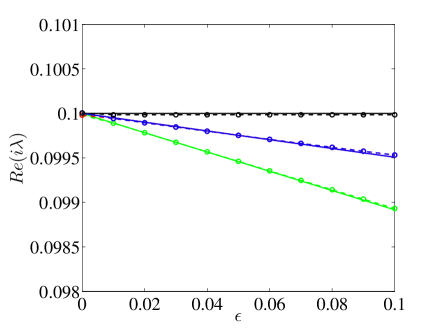
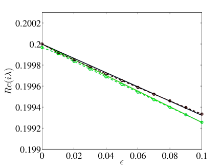
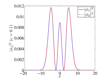
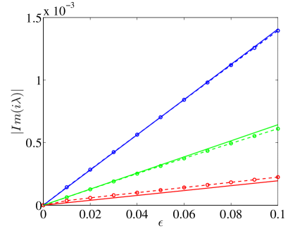
Figure 20: Case of $a=b=1,g_{11}=1,g_{12}=0.1,g_{22}=1,\Omega=0.1$ for the $(2,2)$ branch: The top left panel shows the imaginary parts of the eigenvalues around $-i\Omega$ as functions of $\epsilon$ with $O(\epsilon)$ corrections (solid lines) and corresponding numerical results for comparison (dashed lines with circles). The red and green lines are almost identical since one pair of the eigenvalues of $M_{a}$ for $\lambda^{(0)}=-i\Omega$ corresponds to complex conjugates. The top right panel shows the imaginary parts of the eigenvalues around $-i2\Omega$. It should be noticed again that the red lines and green lines (solid and dashed) are essentially identical and the blue lines and black lines (solid and dashed) are almost the same since two quartets of eigenvalues of $M_{a}$ for $\lambda^{(0)}=-i2\Omega$ arise in this case. Moreover, the nonzero real parts of $\lambda$’s also imply the instability of the solution, as shown in the bottom right panel (solid lines for the $O(\epsilon)$ correction using this pair of complex conjugates and the dashed lines for the numerical computation of the real parts of the eigenvalues; green is used for $M_{a}$ for $\lambda^{(0)}=-i\Omega$ while red and blue denote the imaginary parts for the $M_{a}$ with $\lambda^{(0)}=-i2\Omega$ eigenvalues). The densities of $\phi_{1}$ and $\phi_{2}$ at $\epsilon=0.1$ are given in the bottom left panel, showcasing the second excited state nature of both fields.

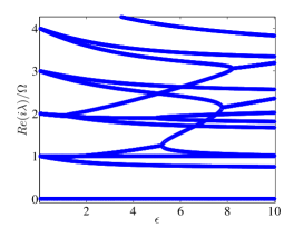
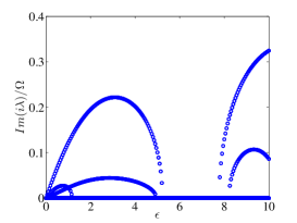
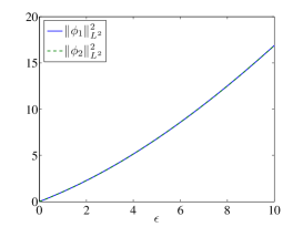
Figure 21: The left (middle) panel shows the change of imaginary (real) parts of the eigenvalues for the $(2,2)$ branch of solutions with $a=b=1,g_{11}=1,g_{12}=0.1,g_{22}=1,\Omega=0.1$. In this case, the middle panel illustrates the potential of the configuration for 3 instabilities all of which are manifested (possibly even concurrently for small $\epsilon$). Interestingly though, for sufficiently large $\epsilon$, there exists a potential parametric interval of spectral stability. In the right panel, we plot the $L^{2}$-norm of the solution of $\phi_{j}$ as a function of $\epsilon$.

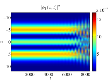
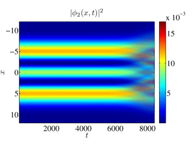
Figure 22: The top left (right) panel shows an example of the dynamics of $|\phi_{1}|^{2}$ ($|\phi_{2}|^{2}$) with $a=b=1,g_{11}=1,g_{12}=0.1,g_{22}=1$, $\Omega=0.1$ and $\epsilon=0.1$. Over longer time scales, the oscillatory instability sets in re-arranging the atomic distribution in both components.

IV.7 Summary of the spectral stability results

In Section IV, we have examined solutions with different $(m,n)$ pairs for $0\leq m,n\leq 2$. The spectral stability of each solution has been studied both analytically and topologically via perturbation theory for small $\epsilon$. The topological results are robust, and valid for all pairs of $(m,n)$. In order to upgrade the stability results for general $(m,n)$, we first introduce several identities for $m,n\geq 1$ as follows:

$$\alpha_{m}:=\frac{A_{m}-2B_{m,m+1}}{D_{m,m,m-1,m+1}}=\frac{D_{m,m,m-1,m+1}}{A_{m}-2B_{m,m-1}}=-\sqrt{\frac{m}{m+1}}$$ (25)

$$\frac{D_{m,n,m+1,n+1}+\alpha_{n}\cdot D_{m,n,m+1,n-1}}{B_{m,n}-B_{m+1,n}}=\frac{D_{m,n,m-1,n+1}+\alpha_{n}\cdot D_{m,n,m-1,n-1}}{\alpha_{m}(B_{m,n}-B_{m-1,n})}=\sqrt{\frac{m+1}{n+1}}$$ (26)

$$\frac{B_{0,n-1}-B_{0,n}}{D_{0,1,n-1,n}}=-\frac{1}{\alpha_{n}}\frac{B_{0,n}-B_{0,n+1}}{D_{0,1,n,n+1}}=\frac{1}{\sqrt{n}},\quad B_{0,n}=\frac{(2n-1)!}{(n-1)!\,n!\,2^{2n-1}}\sqrt{\frac{\Omega}{2\pi}}.$$ (27)

Though no analytical proofs for these identities are provided here, we have verified them for general $(m,n)$ pairs through extensive numerical experiments. Then for the stability results:

• When $m>0$, there are four eigenvalues of $-iJ\mathcal{L}$ near $-i\ell\Omega$ for $1\leq\ell\leq m$. According to the Hamiltonian-Krein index, at most two eigenvalues among four can have positive real parts (leading to instability). However, the perturbation calculation suggests that not all of the four eigenvalues can enter the complex plane for $m\geq 1$.

  Remark 1.

  For $1\leq m\leq n$, it can be directly checked using (25)–(26) that $M_{a}$ for $\ell=1$ has an eigenvalue $0$ with eigenvector $\displaystyle{\left(1,\sqrt{\frac{m}{m+1}},\frac{b}{a}\sqrt{\frac{n+1}{m+1}},\frac{b}{a}\sqrt{\frac{n}{m+1}}\right)^{\mathrm{T}}}$.

  Thus, near $-i\ell\Omega$, two eigenvalues will always stay on the imaginary axis (one of them is $0$) and there are at most one pair of complex eigenvalues. We discussed previously the physical origin of the corresponding (dipolar) symmetry removing the potential for one among the pertinent instability eigendirections.

• When $m<n$, there are three eigenvalues near $-i\ell\Omega$ for $m<\ell\leq n$. At most one pair of these eigenvalues will have nonzero real part. Similar to Remark 1, we particularly notice that one of eigenvalues near $-i\Omega$ will always be zero.

  Remark 2.

  For $m=0$ and $1\leq n$, it can be directly checked using (25)–(27) that $M_{b}$ for $\ell=1$ has an eigenvalue $0$ with eigenvector $\displaystyle{\left(\frac{a}{b}\frac{1}{\sqrt{n}},\sqrt{\frac{n+1}{n}},1\right)^{\mathrm{T}}}$.

• The Hamiltonian-Krein index, $K_{\mathrm{Ham}}=2(m+n)$, gives an upper bound for the number of pairs of eigenvalues that can leave the imaginary axis and bring about an instability. In the examined examples, this upper bound can be reached only when $m=0$. For $m>0$, the exact upper bound will be $2(m+n-1)$, given the presence of the symmetry/invariance associated with dipolar motion of the condensate removing one of the potentially unstable associated eigendirections

• When $(m,n)=(0,1)$, an instability will arise if and only if $g_{12}>g_{22}>0$, i.e., the inter-component nonlinear interactions are stronger than the nonlinear interactions within the “dark” species.

As $\epsilon$ grows away from $0$, we notice that the eigenvalue starting from $-i\Omega$ can collide with the eigenvalues from $-i3\Omega$, $-i5\Omega,\dots$ on the imaginary axis to generate eigenvalues with nonzero real part. Similarly, the eigenvalue from $-i2\Omega$ can meet with the eigenvalues from $-i4\Omega,\,-i6\Omega,\dots$ on the imaginary axis to produce new pairs of eigenvalues with nonzero real part. Our numerical results suggest that (given their respective parities) eigenmodes at odd multiples of $\Omega$ interact with other ones such and similarly even ones interact with even. While our analysis does not lend itself to the consideration of this wide parametric regime in $\epsilon$, numerical computations reveal the corresponding potential (oscillatory) instabilities and their customary restabilization for some interval of wider parametric variations of $\epsilon$.

V Conclusions & Future Challenges

In the present work, we illustrated the usefulness of Lyapunov-Schmidt reductions, as well as of Hamiltonian-Krein index theory, in acquiring a systematic understanding of bifurcations from the linear limit of the multi-component system of atomic gases. Here, we have focused on the two-component case, yet it should be evident from the analysis how general multi-component cases will modify the specifics yet not the overall formulation of the present setting. Once again, this mean-field limit may be of somewhat limited applicability to the atomic case for very small atom numbers (mathematically, squared $L^{2}$ norms), as there additional (quantum) effects may skew the picture. Nevertheless, optical settings (with suitably tailored refractive index profiles) can lend themselves to the analysis presented herein. Moreover, and arguably more importantly, the topological nature of the tools developed provides insights on the number of potentially unstable eigendirections even far from the linear limit, where the mean field model has been successfully used to monitor different multi-component excited states, such as most notably e.g. dark-bright solitons and their close relatives (such as dark-dark ones). We have found a number of surprising results in the process, such as the fact that $(0,1)$ states (involving one fundamental and one excited state) may be unstable provided that inter- to intra-component interaction ratios are suitably chosen. Another intriguing feature is that the presence of additional symmetry (embedded in the dipolar motion inside the trap) may prevent particular instability eigendirections from manifesting themselves.

It would be interesting to extend the present considerations to spinor systems that are intensely studied over the past few years in atomic experiments kawueda ; stampueda . Additionally, higher dimensional settings, both two-dimensional ones where vortex-bright and related states have been devised VB , but also three-dimensional ones involving vortex-rings rings and skyrmions ruost or related patterns would be especially interesting to attempt to explore through this methodology, as traditionally the complexity of such states limits the potential for analytical results. Lastly, it does not escape us that an equally interesting and analytically tractable (at least to some degree) limit is that of large chemical potentials where the solitary waves can be treated as particles. Developing a general theory of that limit and connecting that with the low amplitude limit presented herein, would be of particular interest. This would also allow to showcase the connection between the two tractable limits via numerical computations and to confirm the robustness of the topological tools in revealing the potential for instability while traversing the continuum from one to the other limit. Such studies are currently in progress and will be reported in future publications.

Acknowledgements.
P.G.K. gratefully acknowledges support from NSF-DMS-1312856. T.K. gratefully acknowledges support from Calvin College through a Calvin Research Fellowship.

References

- (1) C. Sulem and P.L. Sulem, The Nonlinear Schrödinger Equation, Springer-Verlag (New York, 1999).
- (2) M.J. Ablowitz, B. Prinari, and A.D. Trubatch, Discrete and Continuous Nonlinear Schrödinger Systems, Cambridge University Press (Cambridge, 2004).
- (3) P.G. Kevrekidis, D.J. Frantzeskakis, and R. Carretero-González, The Defocusing Nonlinear Schrödinger Equation, SIAM (Philadelphia, 2015).
- (4) Yu.S. Kivshar and G.P. Agrawal, Optical Solitons: from fibers to photonic crystals, Academic Press (San Diego, 2003).
- (5) E. Infeld, G. Rowlands, Nonlinear Waves, Solitons and Chaos, Cambridge University Press (Cambridge, 1990).
- (6) P.G. Kevrekidis, D.J. Frantzeskakis, and R. Carretero-González (Eds.), Emergent Nonlinear Phenomena in Bose-Einstein Condensates: Theory and Experiment Springer-Verlag (Heidelberg, 2008).
- (7) S.V. Manakov, Sov. Phys. JETP, 38 (1973) 248–253. V.E. Zakharov and S.V. Manakov, Sov. Phys. JETP, 42 (1976) 842–850
- (8) V.E. Zakharov and E.I. Schulman, Physica D, 4 (1982) 270–274.
- (9) L.P. Pitaevskii and S. Stringari, Bose-Einstein Condensation. Oxford University Press (Oxford, 2003).
- (10) V.S. Bagnato, D.J. Frantzeskakis, P.G. Kevrekidis, B.A. Malomed, and D. Mihalache, Rom. Rep. Phys., 67 (2015) 5–50.
- (11) D.S. Hall, M.R. Matthews, J.R. Ensher, C.E. Wieman, and E.A. Cornell, Phys. Rev. Lett., 81 (1998) 1539–1542.
- (12) D.M. Stamper-Kurn, M.R. Andrews, A.P. Chikkatur, S. Inouye, H.-J. Miesner, J. Stenger, and W. Ketterle, Phys. Rev. Lett., 80 (1998) 2027–2030.
- (13) J. Stenger, S. Inouye, D.M. Stamper-Kurn, H.-J. Miesner, A.P. Chikkatur, and W. Ketterle, Nature, 396 (1998) 345–348.
- (14) Y. Kawaguchi and M. Ueda, Phys. Rep., 520 (2012) 253–381.
- (15) D.M. Stamper-Kurn and M. Ueda, Rev. Mod. Phys., 85 (2013) 1191–1244.
- (16) C. Becker, S. Stellmer, P. Soltan-Panahi, S. Dörscher, M. Baumert, E.-M. Richter, J. Kronjäger, K. Bongs, and K. Sengstock, Nature Phys., 4 (2008) 496–501.
- (17) C. Hamner, J.J. Chang, P. Engels, and M.A. Hoefer, Phys. Rev. Lett., 106 (2011) 065302.
- (18) S. Middelkamp, J.J. Chang, C. Hamner, R. Carretero-González, P.G. Kevrekidis, V. Achilleos, D.J. Frantzeskakis, P. Schmelcher, and P. Engels, Phys. Lett. A, 375 (2011) 642–646.
- (19) D. Yan, J.J. Chang, C. Hamner, P.G. Kevrekidis, P. Engels, V. Achilleos, D.J. Frantzeskakis, R. Carretero-González, and P. Schmelcher, Phys. Rev. A, 84 (2011) 053630.
- (20) A. Álvarez, J. Cuevas, F.R. Romero, C. Hamner, J.J. Chang, P. Engels, P.G. Kevrekidis, and D.J. Frantzeskakis, J. Phys. B, 46 (2013) 065302.
- (21) M.A. Hoefer, J.J. Chang, C. Hamner, and P. Engels, Phys. Rev. A, 84 (2011) 041605(R).
- (22) D. Yan, J.J. Chang, C. Hamner, M. Hoefer, P.G. Kevrekidis, P. Engels, V. Achilleos, D.J. Frantzeskakis, and J. Cuevas, J. Phys. B: At. Mol. Opt. Phys., 45 (2012) 115301.
- (23) P.G. Kevrekidis, D.J. Frantzeskakis, arXiv:1512.06754.
- (24) T. Kapitula, P.G. Kevrekidis, Chaos 15, 037114 (2005).
- (25) T. Kapitula, P.G. Kevrekidis and R. Carretero-González, Physica D 233, 112 (2007).
- (26) D. L. Feder, M. S. Pindzola, L. A. Collins, B. I. Schneider, and C. W. Clark Phys. Rev. A 62, 053606 (2000).
- (27) T. Kapitula, K. Promislow, Spectral and dynamical stability of nonlinear waves, Springer-Verla (New York, 2013).
- (28) L. Nirenberg, Topics in nonlinear functional analysis, American Mathematical Society (Providence, 2001).
- (29) T. Kapitula, P. Kevrekidis, Z. Chen, SIAM J. Appl. Dyn. Sys. 5 (4) (2006) 598–633
- (30) M.P. Coles, D.E. Pelinovsky, P.G. Kevrekidis, Nonlinearity 23, 1753 (2010).
- (31) V.M. Pérez-García and J.J. García-Ripoll, Phys. Rev. A 62, 033601 (2000). D.V. Skryabin, Phys. Rev. A 63, 013602 (2001); R.A. Battye, N.R. Cooper, P.M. Sutcliffe, Phys. Rev. Lett. 88, 080401 (2002). K.J.H. Law, P.G. Kevrekidis, L.S. Tuckerman, Phys. Rev. Lett. 105, 160405 (2010); M. Pola, J. Stockhofe, P. Schmelcher, P.G. Kevrekidis, Phys. Rev. A 86, 053601 (2012).
- (32) S. Komineas, Eur. Phys. J. Spec. Topics, 147 (2007) 133–152. C.F. Barenghi and R.J. Donnelly, Fluid Dyn. Res., 41 (2009) 051401.
- (33) J. Ruostekoski and J. R. Anglin Phys. Rev. Lett. 86, 3934 (2001); C. M. Savage and J. Ruostekoski Phys. Rev. Lett. 91, 010403 (2003).