Singly-Thermostated Ergodicity in Gibbs’ Canonical Ensemble
and the 2016 Ian Snook Prize

Abstract

For a harmonic oscillator, Nosé’s single-thermostat approach to simulating Gibbs’ canonical ensemble with dynamics samples only a small fraction of the phase space. Nosé’s approach has been improved in a series of three steps: [ 1 ] several two-thermostat sets of motion equations have been found which cover the complete phase space in an ergodic fashion; [ 2 ] sets of single-thermostat motion equations, exerting “weak control” over both forces and momenta, have been shown to be ergodic; and [ 3 ] sets of single-thermostat motion equations exerting weak control over two velocity moments provide ergodic phase-space sampling for the oscillator and for the rigid pendulum, but not for the quartic oscillator or for the Mexican Hat potential. The missing fourth step, motion equations providing ergodic sampling for anharmonic potentials requires a further advance. The 2016 Ian Snook Prize will be awarded to the author(s) of the most interesting original submission addressing the problem of finding ergodic algorithms for Gibbs’ canonical ensemble using a single thermostat.

I Gibbs’ Canonical Ensemble

From Gibbs’ 1902 text Elementary Principles in Statistical Mechanics, page 183 :

“If a system of a great number of degrees of freedom is microcanonically distributed in phase, any very small part of it may be regarded as canonically distributed.”

Thus J. Willard Gibbs pointed out that the energy states of a “small” system weakly coupled to a larger “heat reservoir” with a temperature $T$ have a “canonical” distribution :

$$f(q,p)\propto e^{-{\cal H}(q,p)/kT}\ .$$

with the Hamiltonian ${\cal H}(q,p)$ that of the small system. Here $(q,p)$ represents the set of coordinates and momenta of that system.

“ Canonical ” means simplest or prototypical. The heat reservoir coupled to the small system and responsible for the canonical distribution of energies is best pictured as an ideal-gas thermometer characterized by an unchanging kinetic temperature $T$ . The reservoir gas consists of many small-mass classical particles engaged in a chaotic and ergodic state of thermal and mechanical equilibrium with negligible fluctuations in its temperature and pressure. Equilibrium within this thermometric reservoir is maintained by collisions as is described by Boltzmann’s equation. His “H Theorem” establishes the Maxwell-Boltzmann velocity distribution found in the gas. See Steve Brush’s 1964 translation of Boltzmann’s 1896 text Vorlesungen über Gastheorie.

Prior to fast computers texts in statistical mechanics were relatively formal with very few figures and only a handful of numerical results. In its more than 700 pages Tolman’s 1938 tome The Principles of Statistical Mechanics includes only two Figures. [ The more memorable one, a disk colliding with a triangle, appears on the cover of the Dover reprint volume. ] Today the results-oriented graphics situation is entirely different as a glance inside any recent issue of Science confirms.

II Nosé-Hoover Canonical Dynamics – Lack of Ergodicity

In 1984, with the advent of fast computers and packaged computer graphics software already past, Shuichi Nosé set himself the task of generalizing molecular dynamics to mimic Gibbs’ canonical distributionb1 ; b2 . In the end his approach was revolutionary. It led to a new form of heat reservoir described by a single degree of freedom with a logarithmic potential, rather than the infinitely-many oscillators or gas particles discussed in textbooks. Although the theory underlying Nosé’s approach was cumbersome Hoover soon pointed out a useful simplificationb3 ; b4 : Liouville’s flow equation in the phase space provides a direct proof that the “Nosé-Hoover” motion equations are consistent with Gibbs’ canonical distribution. Here are the motion equations for the simplest interesting system, a single one-dimensional harmonic oscillator :

$$\dot{q}=(p/m)\ ;\ \dot{p}=-\kappa q-\zeta p\ ;\ \dot{\zeta}=[\ (p^{2}/mkT)-1\ ]/\tau^{2}\ .$$

The “friction coefficient” $\zeta$ stabilizes the kinetic energy $(p^{2}/2m)$ through integral feedback, extracting or inserting energy as needed to insure a time-averaged value of precisely $(kT/2)$ . The parameter $\tau$ is a relaxation time governing the rate of the thermostat’s response to thermal fluctuations. In what follows we will set all the parameters and constants $(m,\kappa,k,T,\tau)$ equal to unity, purely for convenience. Then the Nosé-Hoover equations have the form :

$$\dot{q}=p\ ;\ \dot{p}=-q-\zeta p\ ;\ \dot{\zeta}=p^{2}-1\ [\ {\rm NH}\ ]\ .$$

Liouville’s phase-space flow equation, likewise written here for a single degree of freedom, is just the usual continuity equation for the three-dimensional flow of a probability density in the ($q,p,\zeta$) phase space :

$$\dot{f}=(\partial f/\partial t)+\dot{q}(\partial f/\partial q)+\dot{p}(\partial f/\partial p)+\dot{\zeta}(\partial f/\partial\zeta)=-f(\partial\dot{q}/\partial q)-f(\partial\dot{p}/\partial p)-f(\partial\dot{\zeta}/\partial\zeta)\ .$$

This approach leads directly to the simple [ NH ] dynamics described above. It is easy to verify that Gibbs’ canonical distribution needs only to be multiplied by a Gaussian distribution in $\zeta$ in order to satisfy Liouville’s equation.

$$e^{-q^{2}/2}e^{-p^{2}/2}e^{-\zeta^{2}/2}\propto f_{NH}\propto f_{G}e^{-\zeta^{2}/2}\longrightarrow(\partial f_{NH}/\partial t)\equiv 0\ .$$

Hoover emphasized that the simplest thermostated system, a harmonic oscillator, does not fill out the entire Gibbs’ distribution in $(q,p,\zeta)$ space. It is not “ergodic” and fails to reach all of the oscillator phase space. In fact, with all of the parameters ( mass, force constant, Boltzmann’s constant, temperature, and relaxation time $\tau$ ) set equal to unity only six percent of the Gaussian distribution is involved in the chaotic seab5 . See Figure 1 for a cross section of the Nosé-Hoover sea in the $p=0$ plane. The complexity in the figure, where the “holes” correspond to two-dimensional tori in the three-dimensional $(q,p,\zeta)$ phase space, is due to the close relationship of the Nosé-Hoover thermostated equations to conventional chaotic Hamiltonian mechanics with its infinitely-many elliptic and hyperbolic points.

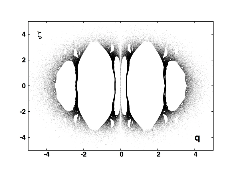
Figure 1: The $p=0$ cross section of the chaotic sea for the Nosé-Hoover harmonic oscillator. 502 924 crossings of the plane are shown. The fourth-order Runge-Kutta integration used a timestep $dt=0.0001$. A point was plotted whenever the product $p_{old}p_{new}$ was negative.

III More General Thermostat Ideas

New varieties of thermostats, some of them Hamiltonian and some not, appeared over the ensuing 30-year period following Nosé’s workb6 ; b7 ; b8 ; b9 ; b10 ; b11 ; b12 ; b13 ; b14 ; b15 ; b16 ; b17 ; b18 . This list is by no means complete. Though important, simplicity is not the sole motivation for abandoning purely-Hamiltonian thermostats. Relatively recently we pointed out that Hamiltonian thermostats are incapable of generating or absorbing heat flowb6 ; b7 . The close connection between changing phase volume and entropy production guarantees that Hamiltonian mechanics is fundamentally inconsistent with irreversible flows.

At equilibrium Brańka, Kowalik, and Wojciechowskib8 followed Bulgac and Kusnezovb9 ; b10 in emphasizing that cubic frictional forces, $-\zeta^{3}p$, which also follow from a novel Hamiltonian, promote a much better coverage of phase space, as shown in Figure 2 . The many small holes in the $p=0$ cross section show that this approach also lacks ergodicity.

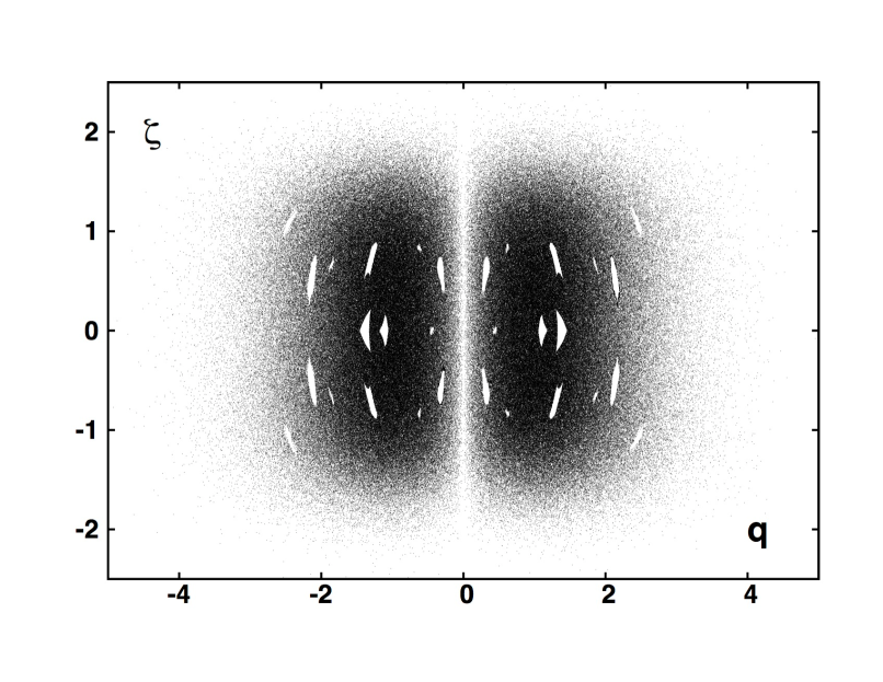
Figure 2: The $p=0$ cross section of the chaotic sea for an oscillator governed by Brańka, Kowalik, and Wojciechowski’s choice of the motion equation, $\ddot{q}=\dot{p}=-q-\zeta^{3}p\ ;\ \dot{\zeta}=p^{2}-1$ . 20 billion timesteps, with $dt=0.0001$, resulted in 636 590 crossings of the $p=0$ section, using the integration procedure of Figure 1.

III.1 Joint Control of Two Velocity Moments

Attempts to improve upon this situation led to a large literature with the most useful contributions applying thermostating ideas with two or more thermostat variablesb9 ; b10 . An example, applied to the harmonic oscillator, was tested by Hoover and Holianb11 and found to provide all of Gibbs’ distribution :

$$\dot{q}=p\ ;\ \dot{p}=-q-\zeta p-\xi p^{3}\ ;\ \dot{\zeta}=p^{2}-1\ ;\ \dot{\xi}=p^{4}-3p^{2}\ {\rm[\ HH\ ]}$$

The two thermostat variables $(\zeta,\xi)$ together guarantee that both the second and the fourth moments of the velocity distribution have their Maxwell-Boltzmann values [ 1 and 3 ] . Notice that two-dimensional cross sections like those in the Figures are no longer useful diagnostics for ergodicity once the phase-space dimensionality exceeds three.

III.2 Joint Control of Coordinates and Velocities

In 2014 Patra and Bhattacharyab12 suggested thermostating both the coordinates and the momenta :

$$\dot{q}=p-\xi q\ ;\ \dot{p}=-q-\zeta p\ ;\ \dot{\zeta}=p^{2}-1\ ;\ \dot{\xi}=q^{2}-1\ {\rm[\ SEPB\ ]}\ .$$

an approach already tried by Sergi and Ezra in 2001b13 .

A slight variation of the Sergi-Ezra-Patra-Bhattacharya thermostat takes into account Bulgac and Kusnezov’s observation that cubic terms favor ergodicity :

$$\dot{q}=p-\xi^{3}q\ ;\ \dot{p}=-q-\zeta p\ ;\ \dot{\zeta}=p^{2}-1\ ;\ \dot{\xi}=q^{2}-1\ {\rm[\ PB_{var}\ ]}\ .$$

These last two-thermostat equations appear to be a good candidate for ergodicity, reproducing the second and fourth moments of $(q,p,\zeta,\xi)$ within a fraction of a percent. We have not carried out the thorough investigation that would be required to establish their ergodicity as the single-thermostat models are not only simpler but also much more easily diagnosed because their sections are two-dimensional rather than three-dimensional.

IV Single-Thermostat Ergodicity

Combining the ideas of “weak control” and the successful simultaneous thermostating of coordinates and momentab14 led to further trials attempting the weak control of two different kinetic-energy momentsb15 . One choice out of the hundreds investigated turned out to be successful for the harmonic oscillator :

$$\dot{q}=p\ ;\ \dot{p}=-q-\zeta(0.05p+0.32p^{3})\ ;\ \dot{\zeta}=0.05(p^{2}-1)+0.32(p^{4}-3p^{2})\ [\ {\rm``0532\ Model^{\prime\prime}}\ ]\ .$$

These three oscillator equations passed all of the following tests for ergodicity :

[ 1 ] The moments $\langle\ p^{2}\ \rangle=1\ ;\ \langle\ p^{4}\ \rangle=3\ ;\ \langle\ p^{6}\ \rangle=15$ were confirmed.

[ 2 ] The independence of the largest Lyapunov exponent to the initial conditions indicated the absence of the toroidal solutions.

[ 3 ] The separation of two nearby trajectories had an average value of 6 :
$\langle\ (q_{1}-q_{2})^{2}+(p_{1}-p_{2})^{2}+(\zeta_{1}-\zeta_{2})^{2}\ \rangle=2+2+2=6$ .

[ 4 ] The times spent at positive and negative values of $\{\ q,p,\zeta\ \}$ were close to equal.

[ 5 ] The times spent in regions with each of the 3! orderings of the three dependent variables were equal for long times.

These five criteria were useful tools for confirming erogidicity. Evidently weak control is the key to efficient ergodic thermostating of oscillator problems.

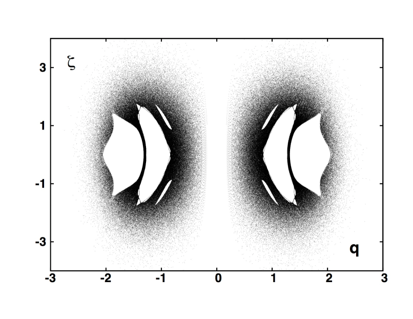
Figure 3: $p=0$ cross section for a singly-thermostated quartic oscillator, with motion equations $\ddot{q}=\dot{p}=-q^{3}-\zeta p^{3}\ ;\ \dot{\zeta}=p^{4}-3p^{2}$ . Runge-Kutta integration as in Figures 1 and 2 with 503 709 crossings of the $p=0$ plane. Several hundred singly-thermostated attempts failed to obtain canonical ergodicity for the quartic oscillator.

V A Fly in the Ointment, the Quartic Potential

The success in thermostating the harmonic oscillator led to like results for the simple pendulum but not for the quartic potentialb15 . See Figure 3. This somewhat surprising setback motivates the need for more work and is the subject of the Ian Snook Prize for 2016. This Prize will be awarded to the author(s) of the most interesting original work exploring the ergodicity of single-thermostated statistical-mechanical systems. The systems are not at all limited to the examples of the quartic oscillator and the Mexican Hat potential but are left to the imagination and creativity of those entering the competition.

Figure 4: Shuichi Nosé ( 1951-2005 ) and Ian Snook ( 1945-2013 )

VI Conclusions – Ian Snook Prize for 2016

It is our intention to reward the most interesting and convincing entry submitted for publication to Computational Methods in Science and Technology ( www.cmst.eu ) prior to 31 January 2017. The 2016 Ian Snook prize of $500 dollars will be presented to the winner in early 2017. An Additional Prize of the same amount will likewise be presented by the Institute of Bioorganic Chemistry of the Polish Academy of Sciences ( Poznan Supercomputing and Networking Center ). We are grateful for your contributions. This work is dedicated to the memories of our colleagues, Ian Snook ( 1945-2013 ) and Shuichi Nosé ( 1951-2005 ), shown in Figure 4 .

References

- (1) S. Nosé, “A Unified Formulation of the Constant Temperature Molecular Dynamics Methods”, Journal of Chemical Physics 81, 511-519 (1984).
- (2) S. Nosé, “Constant Temperature Molecular Dynamics Methods”, Progress in Theoretical Physics Supplement 103, 1-46 (1991).
- (3) Wm. G. Hoover, “Canonical Dynamics: Equilibrium Phase-Space Distributions”, Physical Review A 31, 1695-1697 (1985).
- (4) H. A. Posch, W. G. Hoover, and F. J. Vesely, “Canonical Dynamics of the Nosé Oscillator: Stability, Order, and Chaos”, Physical Review A 33, 4253-4265 (1986).
- (5) P. K. Patra, W. G. Hoover, C. G. Hoover, and J. C. Sprott, “The Equivalence of Dissipation from Gibbs’ Entropy Production with Phase-Volume Loss in Ergodic Heat-Conducting Oscillators”, International Journal of Bifurcation and Chaos 26, 1650089 (2016).
- (6) Wm. G. Hoover and C. G. Hoover, “Hamiltonian Dynamics of Thermostated Systems: Two- Temperature Heat-Conducting Chains”, Journal of Chemical Physics 126, 164113 (2007).
- (7) Wm. G. Hoover and C. G. Hoover, “Hamiltonian Thermostats Fail to Promote Heat Flow”, Communications in Nonlinear Science and Numerical Simulation 18, 3365-3372 (2013).
- (8) A. C. Brańka, M. Kowalik, and K. W. Wojciechowski, “Generalization of the Nosé-Hoover Approach”, The Journal of Chemical Physics 119, 1929-1936 (2003).
- (9) D. Kusnezov, A. Bulgac, and W. Bauer, “Canonical Ensembles from Chaos”, Annals of Physics 204, 155-185 (1990).
- (10) D. Kusnezov and A. Bulgac, “Canonical Ensembles from Chaos: Constrained Dynamical Systems”, Annals of Physics 214, 180-218 (1992).
- (11) Wm. G. Hoover and B. L. Holian, “Kinetic Moments Method for the Canonical Ensemble Distribution”, Physics Letters A 211, 253-257 (1996).
- (12) P. K. Patra and B. Bhattacharya, “A Deterministic Thermostat for Controlling Temperature Using All Degrees of Freedom”, The Journal of Chemical Physics 140, 064106 (2014).
- (13) A. Sergi and G. S. Ezra, “Bulgac-Kusnezov-Nosé-Hoover Thermostats”, Physical Review E 81, 036705 (2010), Figure 2.
- (14) W. G. Hoover, J. C. Sprott, and C. G. Hoover, “Ergodicity of a Singly-Thermostated Harmonic Oscillator”, Communications in Nonlinear Science and Numerical Simulation 32, 234-240 (2016).
- (15) W. G. Hoover, C. G. Hoover, and J. C. Sprott, “Nonequilibrium Systems : Hard Disks and Harmonic Oscillators Near and Far From Equilibrium”, Molecular Simulation ( in press ).
- (16) A. Sergi and M. Ferrario, “Non-Hamiltonian Equations of Motion with a Conserved Energy”, Physical Review E 64, 056125 (2001), Equations 24, 26, and 27. See Reference 18.
- (17) K. P. Travis and C. Braga, “Configurational Temperature and Pressure Molecular Dynamics: Review of Current Methodology and Applications to the Shear Flow of a Simple Fluid”, Molecular Physics 104, 3735-3749 (2006).
- (18) W. G. Hoover, J. C. Sprott, and P. K. Patra,“Ergodic Time-Reversible Chaos for Gibbs’ Canonical Oscillator”, Physics Letters A 379, 2395-2400 (2015).