Autonomous quantum machines and the finite sized Quasi-Ideal clock

Abstract

Processes such as quantum computation, or the evolution of quantum cellular automata are typically described by a unitary operation implemented by an external observer. In particular, an interaction is generally turned on for a precise amount of time, using a classical clock. A fully quantum mechanical description of such a device would include a quantum description of the clock whose state is generally disturbed because of the backreaction on it. Such a description is needed if we wish to consider finite sized autonomous quantum machines requiring no external control. The extent of the backreaction has implications on how small the device can be, on the length of time the device can run, and is required if we want to understand what a fully quantum mechanical treatment of an observer would look like. Here, we consider the implementation of a unitary by a finite sized device which we call the “Quasi-Ideal clock”, and show that the back-reaction on it can be made exponentially small in the device’s dimension with only a linear increase in energy. As a result, an autonomous quantum machine need only be of modest size and energy. We are also able to solve a long-standing open problem by using a finite sized quantum clock to approximate the continuous evolution of an idealised clock. The result has implications for how well quantum devices can be controlled and on the equivalence of different paradigms of control.

I Introduction

Many recent advances in quantum theory are due to our ability to manipulate small systems. Witness on the experimental front, the progress in quantum computation, quantum memory, non-locality, quantum thermodynamics, and randomness generation. The quantum machinery involved in each of these typically requires very precise external control — for example, in a quantum cellular automata, or a quantum computation, a unitary (gate) is applied at each time step.

This is reasonable for modeling a large machine which is controlled by a classical system, but what if we wish to consider a fully quantum machine? This could be an autonomous quantum device which interacts with its surroundings, or a way of modelling a fully quantum observer. While the latter is mostly of foundational interest, the former is needed to understand and optimise current quantum technologies, or understand important physical processes. Take for example, molecular machines or nanomachines such as molecular motors howard1997molecular , which are important in biological processes molecularBio , or distant technologies such as nanorobots nanobots , where quantum effects on the control mechanism, and the back-reaction they incur, are likely to be significant.

Understanding autonomous machines is particularly important in thermodynamics, where one is interested in devices which can be used for tasks such as energy harvesting or erasing a memory Scovil1959masers ; Geusic1967quatum ; linden2010small ; brask2015autonomous ; brandao2013resource ; malabarba2015clock ; tonner2005autonomous ; gelbwaser2014heat ; correa2014quantum ; tonner2007quantum . In the thermodynamics literature, there tend to be two sorts of processes, those which are fully autonomous, and those which allow a certain level of external control at no cost to the agent. A canonical example of the former is the brownian ratchet, popularised by Feynman FeynamnLecs , which simply sits between two thermal baths and extracts work in situ. There are a number of autonomous quantum thermal machines built on this principle linden10 ; brask2015autonomous ; MarcusPauli . However, there are a number of processes, such as quantum Carnot cycles geusic ; gelbwaser2014heat , and thermal operations, on which a number of resource theories are based, and from which one can derive the quantum version of the second law, that require external control. While an autonomous thermal machine can be implemented via a fixed time-independent interaction Hamiltonian, an externally controlled machine requires a time-dependent Hamiltonian. For example, in order to implement a unitary operation, an interaction Hamiltonian must be switched on and allowed to run for a specific amount of time.

Allowing such external control is highly contentious as the hidden cost of such fine-tuned control may often dwarf the perceived costs of such theories. If one insists (as one should) that the true cost of quantum process can only be observed reliable in the absence of external control, a number of questions present themselves - Is there a fundamental disadvantage to autonomous machines as opposed to those with external control? How sensitive are the conclusions of the various “resource theories” to the removal of external control?

Note that if one has access to a system of infinite dimensions and a Hamiltonian unbounded from below, that we may understand as an “idealized clock”, then it turns out that the paradigm of allowing external control vs the paradigm of autonomous machines are equivalent, for instance, see brandao2013resource ; malabarba2015clock . However, while illustrative as a conceptual proof of principle that controlled processes can be turned autonomous, these analyses are misleading for two reasons.

First of all, the Hamiltonian being unbounded from below implies that the clock has infinite energy, which is unphysical. Furthermore, accounting for changes in energy, which is an important part in the analysis of quantum operations, is rendered meaningless in the presence of a control device of infinite energy.

Also, a careful analysis requires one to consider a finite dimensional clock, because it is important to show that an infinite dimensional clock cannot be used to embezzle work from it, an issue covered at length in second . Embezzling of work, based on the notion of entanglement embezzling Hayden-embezzling , is the process of transferring work from a system while only changing the state of the system by an amount (w.r.t. trace distance) which vanishes in the limit of increasing dimension.

Thus, in order to reliably consider the changes in energy and entropy (the two central quantities in thermodynamics) in a controlled quantum process, one requires a physically reasonable control of both finite size and energy, and take into account the back-reaction on it. In fact, there is a wealth of interesting physics that presents itself when we recognize the finiteness of control systems, such as the advantage of coherence in control HesenbergLim , the tradeoff between accuracy and power in thermodynamics MarcusPauli , as well as fundamental bounds on the synchronization time of clocks sandraAlternative .

There are two important limitations of finite clocks. The first is that they can only record the precise time at discrete intervals Peres , and can be very inaccurate in between. Furthermore, any attempt to use the clock to measure time or as a control system disturbs the clock Peres ; buzek ; allcock1969time , leading to the performance of the clock degrading on further use.

In this paper we are able to circumvent these two difficulties. We present a finite size quantum clock, based upon the Hamiltonian of the Wigner clock SaleckerWigner , but whose initial state is a coherent superposition w.r.t. the basis that Peres used Peres . To demonstrate the clock’s utility, we describe how to convert two of the most ubiquitous externally controlled operations in quantum theory: the unitary, and the time-dependent interaction Hamiltonian, into an operation performed by an autonomous device. We compute the back-reaction on the clock, and find analytic bounds on the errors developed in the clock and target system, thus explicitly accounting for the cost of these operations that form the basis of so many theoretical paradigms. Our main result is that we find that the disturbance in the clock can be made exponentially small in the dimension of the clock, a calculation which requires going beyond perturbation theory. We thus see that the back-reaction can be made negligible, and one can make a device autonomous using a control of modest size as well as energy. One significance of this result, is that it allows an autonomous machine, even one of small size, to run for a significant length of time, before becoming too degraded.

In fact, we demonstrate that the evolution of the clock mimics that of the idealized clock (up to the exponentially small error). As such, if one wishes to convert any quantum operation with external control into an autonomous process, one may do so by using the idealized momentum clock (as in malabarba2015clock ), whose description is simple, and keep track of the real error by using the results presented in this manuscript. Thus one can account for the cost of turning a quantum process autonomous without having to explicitly describe the control, an immense advantage for the cases wherein to do so would be either analytically intractable, or computationally intensive maxclock .

On a foundational note, the behaviour of an idealized quantum clock is equivalent to it obeying the canonical commutation relation. Given a suitable definition of a time operator we demonstrate that our finite clock states also approximate the canonical commutator relation — a property which is absent in the clock proposed by SaleckerWigner ; Peres . Importantly, this property, together with the quasi-ideal evolution of our clock, are both consequences of the coherent nature of the clock state. This highlights the importance of quantum coherence in quantum clocks and control.

Organisation of this manuscript. - Given the high volume of material presented, we summarize the main results and discussion first; including a conclusion, and provide the full theorems and technical proofs thereafter. To begin with, Section II introduces the infinite dimensional clock highlighting its relevant properties that we wish to mimic. This is followed by an introduction to finite clocks in Section III, in particular to the complex Gaussian superposition that we study. The main results of our work are then stated and explained in Section IV, including a discussion on the implications for quantum autonomous control in Subsection IV.3. This is followed by a general discussion and conclusions in Sections V and VI respectively. In the main text we prove the results presented in this manuscript. The results themselves are presented with more generality in the form of theorems. The organization of the main text is described directly after the conclusions (Section VI).

II The idealised quantum clock and its properties

The notion of an ideal clock is closely related to whether there exists a time operator in quantum mechanics (i.e. time is an observable). Wolfgang Pauli pauli1 ; pauli2 argued that if there exists an ideal clock with Hamiltonian $\hat{H}$ and ideal observable of time $\hat{t}$; both self-adjoint on some suitably defined domains, then in the Heisenberg picture the pair must obey

$$\frac{d}{dt}\hat{t}(t)={\mathbbm{1}},\quad\forall\,t\in{\mathbbm{R}},$$ (1)

which in turn implies the canonical commutation relation $-\mathrm{i}[\hat{t}(t),\hat{H}]={\mathbbm{1}},\quad\forall t\in{\mathbbm{R}}$ (we use units so that $\hbar=1$) on some suitably defined domain. Pauli further argued that the only pair of such operators (up to unitary equivalence) are $\hat{t}=\hat{x}$ and $\hat{H}=\hat{p}$, where $\hat{x}$, $\hat{p}$ are the canonically conjugate position-momentum operators of a free particle in one dimension. However, all such representations of $\hat{p}$ for which Eq. (1) is satisfied have spectra unbounded from below. One can thus conclude that no perfect time operator exists in quantum mechanics since such clock Hamiltonians would require infinite energy to construct due to the lack of a ground state. The question of whether a physically realizable perfect time operator exists in quantum mechanics is still a contentious issue, see Remark A.1. We will not dwell upon this issue here, but rather summarize the characteristic properties of such a system that allow for the precise timing of events,which we then mimic using a finite sized clock.

For the simple case in which $\hat{t}=\hat{x}_{c}$, $\hat{H}=\hat{p}_{c}$ are the position and momentum operators of a free particle in one dimension, the dynamics are easily solvable. We refer to this as the idealised clock. It has three critical properties (that we proceed to discuss in detail), namely:

• The clock possesses a distinguishable basis of “time states”,

• it demonstrates “continuity”, and

• it allows for perfect continuous autonomous control on an external system.

To be more precise, given that the Hamiltonian of the clock is $\hat{H}=\hat{p}_{c}$, the generalised eigenvectors of the position operator $\ket{x}$ are a distinguishable basis of time states by which we mean $\braket{x}{x^{\prime}}=\delta(x-x^{\prime})$, and that given any initial generalized eigenvector $\ket{x}$, the natural evolution of the clock will past through all of the positions $x^{\prime}>x$,

$$e^{-\mathrm{i}t\hat{H}}\ket{x}=\ket{x+t},$$ (2)

i.e. a time translation is equivalent to a spatial translation.

For the second property, note that the equivalence between time and space translations hold for any state of the clock,

$$\braket{x}{e^{-\mathrm{i}t\hat{H}}}{\Psi}=\braket{x-t}{\Psi}.$$ (3)

The fact that this statement holds for all $x,t\in{\mathbbm{R}}$, and in particular, for arbitrarily small $t$ is what we refer to as continuity, or by referring to the clock as continuous.

To demonstrate the third property, that of perfect control, observe that if one adds a position-dependent potential to the clock, it still remains continuous, while its state is only modified by a phase that depends on the potential,

$$\braket{x}{\mathrm{e}^{-\mathrm{i}t\left(\hat{H}+V(\hat{x}_{c})\right)}}{\Psi}=\mathrm{e}^{-\mathrm{i}\int_{x-t}^{x}V(x^{\prime})dx^{\prime}}\braket{x-t}{\Psi},\quad x,t\in{\mathbbm{R}},\,V\in D_{0}.\ref{domainxp}$$ (4)

Notice that the phase integrates over the potential in the region that the state passes through ($[x-t,x]$). The clock can therefore be turned into a control device by simply having the potential be an interaction on an external system, whose strength is a function of the clock’s position. Rather than an observer having to switch on and off an interaction on a system, here the clock does so autonomously by passing through the region of the potential.

A detailed proof of the above statements may be found in Section A, while the consequences for autonomous control of external systems is discussed in IV.4.

III A finite clock to mimic the idealised clock

The clock we propose is based upon a quantum system that has been discussed before in SaleckerWigner ; Peres . The system has dimension $d$ and equally spaced (normalised) energy eigenstates $\ket{E_{n}}$, i.e. its Hamiltonian is

$$\hat{H}_{c}=\sum_{n=0}^{d-1}n\omega\ket{E_{n}}\!\!\bra{E_{n}}.$$ (5)

The frequency $\omega$ determines both the energy spacing as well as the time of recurrence of the clock, $T_{0}=2\pi/\omega$, as $e^{-i\hat{H}_{c}T_{0}}={\mathbbm{1}}_{c}$. This system possesses a distinguishable basis of time states $\left\{\ket{\theta_{k}}\right\}_{k=0}^{d-1}$, that is mutually unbiased w.r.t. the energy eigenstates,

$$\ket{\theta_{k}} =\frac{1}{\sqrt{d}}\sum_{n=0}^{d-1}e^{-i2\pi nk/d}\ket{E_{n}}.$$ (6)

It will also be useful later to have the range of $k$ extended to ${\mathbbm{Z}}$. Extending the range of $k$ in Eq. (6) it follows that $\ket{\theta_{k}}=\ket{\theta_{k\textup{ mod. }d}}$ for $k\in{\mathbbm{Z}}$. The $\ket{\theta_{k}}$ are referred to as time states because they rotate into each other in regular time intervals of $T_{0}/d$, i.e. $e^{-i\hat{H}_{c}T_{0}/d}\ket{\theta_{k}}=\ket{\theta_{k+1}}$. Since they also form an orthonormal basis, this property is true for any state $\ket{\Psi}$ of the clock Hilbert space,

$$\braket{\theta_{k}}{e^{-i\hat{H}_{c}m\,T_{0}/d}}{\Psi}=\braket{\theta_{k-m}}{\Psi},\quad k,m\in{\mathbbm{Z}}.$$ (7)

This is reflective of the idealised case Eq. (3), but the key difference is that for the finite clock, Eq. (7) only holds at regular intervals ($m\in\mathbb{Z}$). Thus while every state of the clock is regular with respect to time, a general clock state does not demonstrate continuity. In fact the time-states $\ket{\theta_{k}}$ themselves are considerably discontinuous. Specifically, as a time-state evolves, it spreads out considerably in the time basis for non-integer intervals Gross2012 ; sergedft . Additionally, the time-states fail to even approximate the canonical commutator relationship between a (suitably defined) time operator and Hamiltonian in any limit Peres . See Section B for a more precise discussion of the behaviour of time-states $\ket{\theta_{k}}$.

The clock that we work with henceforth, rather than being a time-state, is instead a coherent complex Gaussian superposition of time-states,

$$\ket{\Psi_{\textup{nor}}(k_{0})} =\sum_{\mathclap{\begin{subarray}{c}k\in\mathcal{S}_{d}(k_{0})\end{subarray}}}\psi_{\textup{nor}}(k_{0};k)\ket{\theta_{k}},$$ (8)

$$\text{where}\quad\psi_{\textup{nor}}(k_{0};x) =Ae^{-\frac{\pi}{\sigma^{2}}(x-k_{0})^{2}}e^{i2\pi n_{0}(x-k_{0})/d}.$$ (9)

For reasons which will become clear, we refer to these states as Quasi-Ideal clock states. The precise definition and basic properties of these states are detailed in Section VII. Roughly, $k_{0}\in{\mathbbm{R}}$ represents the mean position of the clock about which the Gaussian is centred ($\mathcal{S}_{d}(k_{0})$ is a set of $d$ consecutive integers centered about $k_{0}$, such that the set $\{\ket{\theta_{k}}:k\in\mathcal{S}_{d}(k_{0})\}$ forms a complete orthonormal basis for the clock Hilbert space). $\sigma$ denotes the width of the state in the time basis, ranging from $\sigma\approx 0$ (approximately a time-state) to $\sigma\approx d$ (almost an energy eigenstate). $n_{0}\in(0,d-1)$ represents the mean energy number of the clock, so that the average energy $\omega n_{0}$ ranges between $0$ and $\omega(d-1)$. $A$ is a normalisation constant.

In the next section we quantify how closely a clock state of the above form mimics the behaviour of an idealised clock, and the consequences for using the clock as a control device.

IV Results (Overview)

We now briefly state and explain our main results, reserving the full theorems for later. For simplicity, we state here the results for the simplest case of the clock state, where $\sigma=\sqrt{d}$, and $n_{0}=(d-1)/2$. This corresponds to a state, that when expressed in the energy eigenbasis, has a width (i.e. the standard deviation w.r.t. the energy spacing $\omega$) that is also approximately $\sqrt{d}$, and whose mean energy is at about the middle of the energy spectrum. We discuss the more general case in Section V. In the following, we use $poly(d)$ to refer to a polynomial in $d$ and use $\mathcal{O}$ for Big-O notation.

IV.1 Quasi-Continuity

Our first result is to recover the continuity of a quantum clock for the class of complex Gaussian superpositions of time-states introduced above.

Result 1 (See Theorem VIII.1 for the most general version).

If the clock begins in a complex Gaussian superposition centred about $k_{0}$, i.e. $\braket{\theta_{k}}{\Psi_{\textup{nor}}(k_{0})}=\psi_{\textup{nor}}(k_{0};k)$, then for all $k\in\mathcal{S}_{d}(k_{0}+t\,d/T_{0})$ and $t\in{\mathbbm{R}}$,

$$\begin{split}\braket{\theta_{k}}{e^{-\mathrm{i}t\hat{H}_{c}}}{\Psi_{\textup{nor}}(k_{0})}&=\psi_{\textup{nor}}(k_{0}-d\frac{t}{T_{0}};k)+\braket{\theta_{k}}{\epsilon_{c}},\\ \text{where}\quad|\!\braket{\theta_{k}}{\epsilon_{c}}\!|&\leq\varepsilon_{c}(t,d)=\mathcal{O}\left(t\;poly(d)\;e^{-\frac{\pi}{4}d}\right)\,\textup{as }d\rightarrow\infty.\end{split}$$ (10)

In other words, the evolution of the clock state, which is composed of the discrete coefficients $\braket{\theta_{k}}{e^{-\mathrm{i}t\hat{H}_{c}}}{\Psi_{\textup{nor}}(k_{0})}$, may be approximated by the continuous movement of the background Gaussian function $\psi_{\textup{nor}}(k_{0};x)$ (see Fig. 1 a). This mimics the equivalence of time and space translations of the idealised clock, Eq. (3), and crucially holds for arbitrarily small time intervals $t$, in contrast to a clock that is a single time state $\ket{\theta_{k}}$. The error in the approximation is bounded to be linear in time, but exponentially small in the dimension.

From another perspective, our set-up can be viewed as a specific example of a continuous time quantum walk. The authors of Gross2012 studied such walks when the initial state has support on a fixed subset of $\{\ket{\theta_{k}}\}_{k=0}^{d-1}$, and showed that the support of the state necessary spreads out to occupy the entire space $\{\ket{\theta_{k}}\}_{k=0}^{d-1}$ in finite time. The above result demonstrates, that these no-go theorems can be circumvented for some states whose support is exponentially suppressed in regions away from a central region.

IV.2 Autonomous Quasi-Control

For the clock to serve as a quantum control unit, it must be continuous not only under its own evolution, but also in the presence of an appropriate potential, as in the case of the idealised clock (4). Our main result is to prove a similar behaviour for the finite clock.

Result 2 (See Theorem IX.1 for the most general version).

Let $V_{0}:{\mathbbm{R}}\rightarrow{\mathbbm{R}}$ be an infinitely differentiable, periodic function with period $2\pi$, normalized so that its integral over a period is $\Omega$, with $-\pi\leq\Omega<\pi$. For the finite clock of dimension $d$, construct a potential from $V_{0}$ as follows,

$$\hat{V}_{d} =\frac{d}{T_{0}}\sum_{k=0}^{d-1}{V}_{d}(k)\ket{\theta_{k}}\!\!\bra{\theta_{k}}, \quad V_{d}(x) =\frac{2\pi}{d}V_{0}\left(\frac{2\pi x}{d}\right).$$ (11)

Then under the Hamiltonian $\hat{H}_{c}+\hat{V}_{d}$, if the clock begins in a complex Gaussian superposition $\braket{\theta_{k}}{\Psi_{\textup{nor}}(k_{0})}=\psi_{\textup{nor}}(k_{0};k)$, then for all $k\in\mathcal{S}_{d}(k_{0}+t\,d/T_{0})$ and $t\in{\mathbbm{R}}$,

$$\begin{split}\braket{\theta_{k}}{e^{-\mathrm{i}t(\hat{H}_{c}+\hat{V}_{d})}}{\Psi_{\textup{nor}}(k_{0})}=&\,\mathrm{e}^{-\mathrm{i}\int_{k-d\,t/T_{0}}^{k}V_{d}(x)dx}\,\psi_{\textup{nor}}(k_{0}-d\frac{t}{T_{0}};k)+\braket{\theta_{k}}{\epsilon_{v}},\\ \;\;\;\;\;\text{where}\quad|\!\braket{\theta_{k}}{\epsilon_{v}}\!|&\leq\varepsilon_{v}(t,d)=\,\mathcal{O}\left(t\;poly(d)\;e^{-\frac{\pi}{4}\frac{d}{\zeta}}\right)\,\textup{as }d\rightarrow\infty,\end{split}$$ (12)

where $\zeta\geq 1$ is a measure of the size of the derivatives of $V_{0}(x)$,

$$\begin{split}\zeta&=\left(1+\frac{0.792\,\pi}{\ln(\pi d)}b\right)^{2},\quad\text{for any }\\ b&\geq\;\sup_{k\in{\mathbbm{N}}^{+}}\left(2\max_{x\in[0,2\pi]}\left|V_{0}^{(k-1)}(x)\right|\,\right)^{1/k},\end{split}$$ (13)

where $V_{0}^{(k)}(x)$ is the $k^{\textup{th}}$ derivative with respect to $x$ of $V_{0}(x)$. Roughly speaking - the larger the derivatives, the larger is $\zeta$. [see Fig. 1 b].

Note the construction of the potential is analogous to the case of the idealised clock; there the potential is expressed in the conjugate variable ($\hat{x}_{c}$) to the Hamiltonian ($\hat{p}_{c}$); in the case of the finite clock the potential is diagonal in a basis (of time states) that is mutually unbiased w.r.t. the energy eigenbasis.

As in the case of the idealised clock, this result allows one to implement a unitary on an external system, or any time-dependent interaction that commutes with the Hamiltonian of the system. We discuss this in greater detail in Section IV.4, and bound the errors in the system and the clock at the end of such processes (in comparison to the idealised case). In particular, we will show that the state of the clock is disturbed by only an exponentially small amount in the dimension of the clock.

The clock as a switch. - Note that in the case of the idealised clock, the “steepness” of the potential (i.e. the magnitude of the derivatives) does not affect the continuity of the clock, i.e. do not enter in Eq. (4). Thus there is no limit to how quickly the idealised clock could switch on and off an interaction on an external system. This is no longer the case for the finite clock, since the steeper the potential, the larger the error in the continuity of the clock. In the discussion of the clock as a control device in Section IV.4, we will see how the above result leads to a natural tradeoff between how sharply the clock can switch on and off interactions on the one hand, vs the back-reaction on the clock and accuracy of the process implemented on the external system on the other hand.

In further work RMRenatoetal , it is demonstrated that the result above (in it’s more general form presented in Theorem IX.1) also encapsulates continuous weak measurements on the state of the clock, that may be used to extract temporal information from the clock (i.e. to measure time).

To conclude this section, we will briefly point out how this work is related to the so-called Pegg and Barnet phase operator, $\hat{\Phi}_{\textup{PB}}=\sum_{k=0}^{d-1}\left(\vartheta_{0}+\frac{2\pi}{d}k\right)\ket{\theta_{k}}\!\!\bra{\theta_{k}}$, $\vartheta_{0}\in{\mathbbm{R}}$ PeggBarnet89 . In particular, we see that the potential $\hat{V}_{d}$ is a function of it. Specifically $\hat{V}_{d}=\omega V_{0}\left(\hat{\Phi}_{\textup{PB}}-\vartheta_{0}{\mathbbm{1}}_{d}\right)$. Note that the Phase operator $\hat{\Phi}_{\textup{PB}}$ was introduced by A. Peres under the name of a time operator $\hat{t}_{c}$, approximately 10 years prior to Pegg and Barnet, as we will see in Section IV.3.

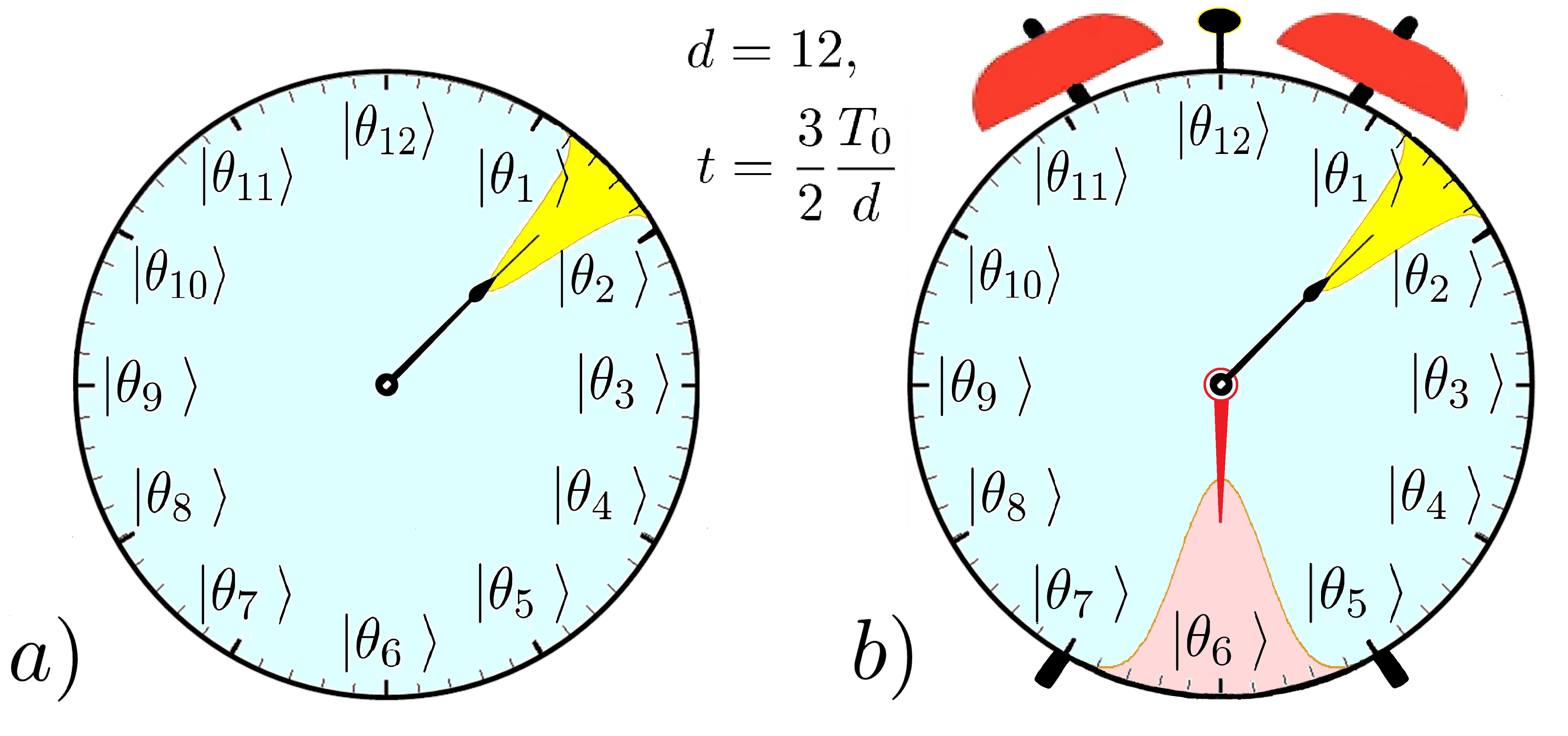
Figure 1: Resemblance of a quantum clock to a classical clock. a) Illustration of main result 1. A quantum clock state $\ket{\Psi_{\textup{nor}}(12)}$ initially centered at “12 o’clock” time evolved to $t=3T_{0}/(2d)$. The clock state moves continuously around the clock face, maintaining an approximately constant width, in contrast to the behaviour of time states $\ket{\theta_{k}}$. b) Illustration of main result 2. Now a potential peaked around “6 o’clock” is introduced. The clock dynamics will be, up to a small error the same as in a) until a time just before “6 o’clock”, at which point the clock will start to acquire a phase due to its passage over the potential. At a time just after “6 o’clock”, the dynamics will start to resemble those of a) again, but now with a global phase added. A direct consequence of main result 2, is that one can use such a potential to induce a time dependent phase that can control an auxiliary quantum system, resembling the working of an alarm clock.

IV.3 Quasi-Canonical Commutation

So far we have demonstrated that the finite dimensional Quasi-Ideal clock state, Eq. (8), satisfies the three properties of the idealized clock, up to a small quantifiable error. Recall that for the idealized clock, these desired properties were a direct consequence of the existence of a perfect time operator, Eq. (1), which is satisfied if $[\hat{t},\hat{H}]=\mathrm{i}$ on some appropriately defined domain. We now discuss the issue of the commutator. For the finite clock, since the $\ket{\theta_{k}}$ rotate into each other in regular time intervals, an intuitive definition of a time operator is in the eigenbasis of $\ket{\theta_{k}}$. Therefore, in analogy to the energy operator, $\hat{H}_{c}$, we define the time operator Peres

$$\hat{t}_{c}=\sum_{k=0}^{d-1}k\frac{T_{0}}{d}\ket{\theta_{k}}\!\!\bra{\theta_{k}}.$$ (14)

However, as noted by A. Peres Peres , this operator cannot obey $[\hat{t}_{c},\hat{H}_{c}]=\mathrm{i}$ for any time state $\ket{\theta_{k}}$. In fact,

$$\bra{\theta_{k}}[\hat{t}_{c},\hat{H}_{c}]\ket{\theta_{k}}=0\quad\text{for all }k\in{\mathbbm{Z}}\text{ and }d\in{\mathbbm{N}}^{+}.$$ (15)

This is intrinsically related to the time-states not being good clocks themselves. However, while the time and energy operators cannot obey the canonical commutation relation themselves, they do approximate it when applied to the subspace of clock states that we propose. Specifically, for complex Gaussian superpositions of time states $\ket{\Psi_{\textup{nor}}(k_{0})}$,

Result 3 (See Theorem XI.1 for the most general version).

$$\begin{split}[\hat{t}_{c},\hat{H}_{c}]\ket{\Psi_{\textup{nor}}(k_{0})}&=\mathrm{i}\ket{\Psi_{\textup{nor}}(k_{0})}+\ket{\varepsilon_{\textup{comm}}},\\ \text{where}\quad\|\ket{\varepsilon_{\textup{comm}}}\|_{2}&=\mathcal{O}\left(poly(d)\;\mathrm{e}^{-\frac{\pi}{4}d}\right)\,\textup{as }d\rightarrow\infty.\end{split}$$ (16)

The implication of Eq. (16) is that our Quasi-Ideal clock states $\ket{\Psi(k_{0})}$ can achieve the canonical commutation relation up to a exponentially small error in clock dimension. In addition, since the l.h.s. of Eq. (16) is $T_{0}$ independent, so is the error $\|\ket{\varepsilon_{\textup{comm}}}\|_{2}$.

See Remark XI.1 that relates the above result to previous work on approximating the canonical commutator relation in finite dimension.

IV.4 Consequences of Autonomous Quasi-control

We now discuss the important consequences that Result 2 has for quantum control. Consider a quantum system of dimension $d_{s}$, upon which we require a unitary $\tilde{U}$ to be implemented within a time interval $t\in[t_{1},t_{2}]$. More precisely, we would like that for any initial state $\rho_{s}\in\mathcal{S}(\mathcal{H}_{s})$,

$$\rho_{s}(t)=\begin{cases}\rho_{s}&\mbox{ if }0\leq t<t_{1}\\ \tilde{U}\rho_{s}\tilde{U}^{\dagger}&\mbox{ if }t>t_{2}.\end{cases}$$ (17)

Such an operation could represent, for example, the implementation of a quantum gate in a quantum computer. The operation can be implemented by applying an interaction on the system in the given time interval, for instance via the time dependent Hamiltonian $\hat{H}(t)=\hat{H}_{s}^{int}g(t)$ acting on $\mathcal{H}_{s},$ where $\tilde{U}=\mathrm{e}^{\mathrm{i}\hat{H}^{int}_{s}},$ and $g\in L({\mathbbm{R}}:{\mathbbm{R}}_{\geq 0})$ is a normalised pulse within the time interval, i.e. $\int_{t_{1}}^{t_{2}}dx\,g(x)=1,$ with support $[t_{1},t_{2}]$. Indeed, the state of the system is found to be

$$\rho_{s}(t) =U(t)\rho_{s}U^{\dagger}(t),\quad\text{where}\quad U(t)=\mathrm{e}^{-\mathrm{i}\hat{H}_{s}^{int}\int_{0}^{t}dxg(x)},$$ (18)

thus implementing the desired unitary Eq. (17). However, the interaction Hamiltonian $\hat{H}(t)$ is time dependent, and the pulse $g(t)$ represents an external observer modulating its strength, which makes the entire operation non-autonomous.

One can describe the above autonomously by using the idealized (albeit unphysical) clock, as in malabarba2015clock , by having the pulse $g(t)$ modulated by the clock itself, as a position dependent potential $g(x)$. In Section X.2, we demonstrate that for the idealized clock there is no back-reaction due to the potential, and the unitary $\tilde{U}$ is implemented perfectly.

We now show that a direct consequence of the autonomous quasi-control result, is that the unitary can be implemented autonomously with the aid of the finite clock, while only incurring a small error due to the finite nature of the clock. This is done analogously to the idealised case, by implementing the pulse $g(t)$ by a potential term $V_{0}$ that is added to the clock’s own Hamiltonian. To be more precise,

Result 4 (See Section X.3 for the proof and explicit construction).

There exists a $V_{0}$ (and an associated $\zeta<\infty$ given by Eq. (13)) such that for all unitaries $\tilde{U}$, initial states $\rho_{s}\in\mathcal{S}(\mathcal{H}_{s})$, and time intervals $t\in[0,t_{1}]\cup[t_{2},T_{0}]$, for all $0<t_{1}<t_{2}<T_{0}$, the evolution of the initial state $\rho_{sc}^{\prime}(0)=\rho_{s}\otimes\ket{\Psi_{\textup{nor}}(0)}\!\!\bra{\Psi_{\textup{nor}}(0)}$ under the time independent Hamiltonian $\hat{H}_{sc}={\mathbbm{1}}_{s}\otimes\hat{H}_{c}+\hat{H}^{int}_{s}\otimes\hat{V}_{d},$ denoted by $\rho_{sc}^{\prime}(t)=\mathrm{e}^{-\mathrm{i}t\hat{H}_{sc}}\,\rho_{sc}^{\prime}(0)\,\mathrm{e}^{\mathrm{i}t\hat{H}_{sc}}$ satisfies

$$\|\rho_{s}(t)-\rho_{s}^{\prime}(t)\|_{1}\leq\sqrt{d_{s}\mathrm{tr}[\rho_{s}^{2}]}\,\Big{(}\varepsilon_{s}(t,d)+\varepsilon_{v}(t,d)\big{(}2+\varepsilon_{v}(t,d)\big{)}\Big{)},$$ (19)

where $\rho_{s}^{\prime}(t)=\mathrm{tr}_{c}[\rho_{sc}^{\prime}(t)]$ denotes the partial trace over the clock, $\rho_{s}(t)$ is given by Eq. (18), and the error $\varepsilon_{s}\geq 0$ is independent of both $\rho_{s}$ and $d_{s}$. The explicit form of $\varepsilon_{s}$, specifying how it depends on the potential $V_{0}$, is provided in Section X, see Corollary X.0.2.

Before discussing Eq. (19) in more detail, we also introduce a dynamical measure of disturbance for the clock. Since the clock state $\rho_{c}^{\prime}(t)=\mathrm{tr}_{s}[\rho_{sc}^{\prime}(t)]$ undergoes periodic dynamics with periodicity $T_{0}$ when no unitary is implemented, i.e. when $V_{0}(x)=0$ for all $x\in{\mathbbm{R}}$, the difference in trace distance between the initial and final state after one period is exactly zero. Moreover, when $V_{0}\neq 0$ any difference between the two states is solely due to the back-reaction caused by the potential implementing the unitary on the system.

A simple application of Result 2, allows for a direct characterization of this disturbance,

$$\|\rho_{c}^{\prime}(0)-\rho_{c}^{\prime}(T_{0})\|_{1}\leq 2\,\varepsilon_{v}(T_{0},d).$$ (20)

Eqs. (19) and (20), represent a trade-off between the back-reaction on the clock dynamics on the one hand, and how well the clock acts as a switch on the other hand. The back-reaction $\varepsilon_{v}$ (introduced in Eq. 12) is minimized by having the potential $V_{0}$ be as “gradual” as possible (i.e. small $\zeta$). However, the error $\varepsilon_{s}$ is minimized by having the unitary implemented as much as possible only within the time interval $[t_{1},t_{2}]$, and this requires a narrower (and thus steeper) potential (i.e. large $\zeta$). See Fig. 2 for a visual discussion of the effect of the potential on the two error terms.

We can also investigate how the tradeoff depends on $d$. Depending on how one parametrizes the potential $V_{0}$ with $d$, the decay rates of $\varepsilon_{v}$ and $\varepsilon_{s}$ as a function of $d$ will be different. We highlight here two extremal cases. The first case is that of minimal clock disturbance. This corresponds to when we fix the tolerance error $\varepsilon_{s}$ to be independent of $d$, for all $\varepsilon_{s}>0$. In this case $V_{0}$ can be chosen to be $d$ independent from which it follows that (refer Eqs. 12,13) $b$ is constant and $\lim_{d\rightarrow\infty}\zeta=1$, meaning that the clock disturbance $\varepsilon_{v}$ is minimal and has a decay rate asymptotically equal to that given by the quasi-continuity bound $\varepsilon_{c}$ (See Eq. (10)). More generally, we show that one can even achieve a parametrisation such that $\lim_{d\rightarrow\infty}\varepsilon_{s}=0$ while still maintaining $\lim_{d\rightarrow\infty}\zeta=1$.

Alternatively, one can choose a potential with the aim of minimizing the r.h.s. of Eq. (19). This leads to both $\|\rho_{s}(t)-\rho_{s}^{\prime}(t)\|_{1}$ and $\|\rho_{c}^{\prime}(0)-\rho_{c}^{\prime}(T_{0})\|_{1}$ to be of the same order and to decay faster than any power of $d$, specifically, exponential decay in $d^{1/4}\sqrt{\ln d}$.

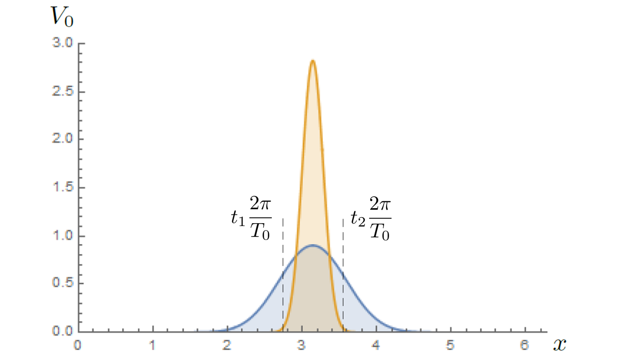
Figure 2: Plot of the potential $V_{0}(x)=A_{c}\cos^{2n}\left(\frac{x-\pi}{2}\right)$ over one period $[0,2\pi]$, with $A_{c}$ a normalisation constant, where $n=10$ (blue), and $n=100$ (orange). The blue potential is “flatter” than the orange potential, and as such, $b$ in Eq. (13) is smaller than in the case of the orange potential. The disturbance $\varepsilon_{v}$ in the clock’s dynamics caused by the implementation of the unitary (see Eq. (20)), will be smaller for the blue potential than for the orange potential. However, the error term $\varepsilon_{s}$ involved in implementing the system unitary (see Eq. (19)), will be larger for the blue potential than for the orange potential. Generally speaking, whenever $b$ is larger, $\varepsilon_{s}$ can be made smaller at the expense of a larger disturbance to the clock’s dynamics (i.e. larger $\varepsilon_{v}$). This trade off is reminiscent of the information gain disturbance principle info_disturbace_Paul , but here rather than gaining information, the unitary is implemented more accurately (i.e. smaller r.h.s. in Eq. (19)).

IV.5 Results for Quasi-Ideal clock states of general width

So far, the results stated have only been for when the initial complex Gaussian superposition of time states $\ket{\Psi_{\textup{nor}}(k_{0})}$ has a width $\sigma$ equal to $\sqrt{d}$ and mean energy centered in the middle of the spectrum of $\hat{H}_{c}$. This particular choice of the width which we call symmetric, has a particular physical significance. The uncertainty in both the energy and time basis, denoted $\Delta E$ and $\Delta t$ respectively, are equal with $\Delta E\Delta t=1/2$. The last equality is true regardless of the width $\sigma$, implying that all our Quasi-Ideal clock states are minimum uncertainty states.4 Whenever $\sigma>\sqrt{d}$, we have $\Delta E<\Delta t$ implying less uncertainty in energy. We call these energy squeezed states in analogy with quantum optics terminology. Meanwhile, we call states for which $\sigma<\sqrt{d}$, time squeezed since $\Delta E>\Delta t$ in this case. It is likely that only time squeezed states can achieve the Heisenberg limit HesenbergLim . Yet, from the viewpoint of quantum control, our results suggest that squeezed states (either in the time or energy basis) have larger errors $\varepsilon_{c}$ and $\varepsilon_{v}$, thus rendering them more fragile to back-reactions from the potential $V_{0}$. More precisely, whenever the initial clock state is energy or time squeezed, the error terms $\varepsilon_{c}$, $\varepsilon_{v}$ still maintain their linear scaling with time. However, w.r.t. the dimension of the clock, the error no longer decays exponentially in $d$, but rather in $d^{\eta}$, where $0<\eta<1$, and where $\eta$ decreases as the state is squeezed further in time or energy. (Full details are left to later sections.)

V Discussion and Outlook

Our results have so far been framed in terms of the dimension of the clock. However, since the clock has a Hamiltonian of equally spaced energy levels, the energy of the clock is linear in its dimension. Thus all of our results are also statements on the efficacy of the clock w.r.t. the energy of the state. In particular, this implies that the back-reaction on the clock is exponentially small in its mean energy.

The second question of interest is how does the mean energy of the initial state of the clock effect the errors induced by finite size? From the energy-time uncertainty relation time_energy_PBusch , and indeed the idealised clock, one might expect the larger the mean energy of the state, the better it performs. Contrarily, we find that errors maintain the same exponential decay in $d^{\eta}$ with $\eta=1$ reserved for symmetric states, but now with a smaller prefactor — one has to replace the $\pi/4$ in Eq. (10) with a factor which approaches zero as the mean energy of the initial clock state approaches either end of the spectrum of $\hat{H}_{c}$. This suggests that, when the dimension is finite, it is the dimension itself, rather than the energy of the state, as suggested by the energy-time uncertainty relation time_energy_PBusch , which is the resource for improving the accuracy of a clock.

Thus, an interesting follow-up question to consider is the case of infinite-dimensional Hamiltonians, such as a harmonic oscillator, and investigate the accuracy of the clock w.r.t. to its mean energy. In fact, an alternative interpretation of our results is that the clock Hamiltonian is that of a quantum harmonic oscillator with energy spacing $\omega$, and that we work only in a finite dimensional subspace. In this interpretation, in the error terms $\varepsilon_{c}$, $\varepsilon_{v}$, $\varepsilon_{s}$, one could make the substitution $d\mapsto\frac{2}{\omega}\langle\hat{H}_{c}\rangle$, where $\langle\hat{H}_{c}\rangle$ is the mean energy of the clock’s initial state, $\ket{\Psi_{\textup{nor}}(k_{0})}$. In this case, we can interpret the clock as living in an infinite dimensional Hilbert space and with error terms $\varepsilon_{c}$, $\varepsilon_{v}$ which are exponentially small in mean clock energy.

Based on numerical evidence, we conjecture that the exponential decay of $\varepsilon_{c}$ in the clock dimension for the Quasi-Ideal clock states with $\sigma=\sqrt{d}$, is the best possible scaling with clock dimension which holds for all times in one time period $[0,T_{0}]$. Furthermore, it could be that no initial clock state can achieve a better scaling. Such a fundamental limitation, would have direct implications for how much work can be embezzled from the clock when it implements a unitary in the framework of second . (See Section XII for a longer discussion.)

In the main text we have assumed that the system has a trivial Hamiltonian. The results derived continue to hold in the case of the system having a non-zero $\hat{H}_{s}$, as long as it commutes with the unitary operation being applied, i.e. $[\hat{H_{s}},\tilde{U}]=0$, what is commonly referred to as an “energy-preserving unitary” or “covariant operation”. The results also serve as an approximation for the non-commuting case, if the clock operates at a time-scale much quicker than that of the system (here the frequency of the clock $\omega$, which has so far not affected the results, would become important).

For the general case of non-commuting unitaries, one would additionally need a source of energy and coherence in addition to the source of timing provided by the clock. The energy source can be modeled in our setup explicitly by including a quantum battery system $\mathcal{H}_{b}$ into the setup or taken to be the clock itself. In the former case, the clock would perform an energy preserving unitary over the $\mathcal{H}_{s}\otimes\mathcal{H}_{b}$ system. The battery Hamiltonian and initial state would be such that locally, on $\mathcal{H}_{s}$, an arbitrary unitary would have been performed. Such a battery Hamiltonian and initial battery state has been studied in Aberg , and will be applied to the setup in this paper in an upcoming paper.

VI Conclusions

We solve the dynamics of a finite dimensional clock when the initial state is a coherent complex Gaussian superposition of time states — a basis which is mutually unbiased with respect to the energy eigenstates of the finite dimensional Hamiltonian. We show that such superpositions evolve in time in ways which mimic idealised, infinite dimensional and energy clocks up to errors which decay exponentially fast in clock dimension. We demonstrate the consequences our results have for autonomous quantum control. We show that the clock can implement a timed unitary on the system via a joint clock-system time independent Hamiltonian, with an error which decays faster than any polynomial in the clock dimension; or equivalently, faster than any polynomial in the clock’s mean energy. The implementation of the unitary induces a back-reaction onto the clock’s dynamics, which we prove is also exponentially small in the clock’s dimension and energy. We discuss the trade-off between smaller clock disturbance and better temporal localization of the unitary’s implementation, which our bounds address quantitatively. Our results single out states of equal uncertainty in time and energy, with a mean energy at the mid point of the energy spectrum, as being the most robust, and thus incurring the least disturbance due to its implementation of the unitary on the system.

On another level, by demonstrating that up to small errors, the three core paradigms in quantum control — the unitary (Eq. (17)), the time dependent Hamiltonian (Eq. (18)), and time independent control (Eq. (19)), are all equivalent up to small errors, our results represent a unification of the three paradigms. The implications of this are not only of a foundational nature, but also practical, since it implies that one can numerically simulate a time dependent Hamiltonian on $\mathcal{H}_{s}$, while being re-assured that in actual fact, the results of the simulation are equivalent to simulating a time independent Hamiltonian on the larger Hilbert space $\mathcal{H}_{s}\otimes\mathcal{H}_{c}$, which would be numerically intractable due to the increased dimension.

Such results are important because the implementation of unitaries and time-dependent interactions is a ubiquitous operation encountered in almost every research field of theoretical quantum mechanics; perhaps the most prominent example being in the field of quantum computation. Yet very little was known about how well such control, normally accounted for by a classical field, can actually be implemented by a fully quantum autonomous setup. Our results provide analytical and insightful bounds on exactly how well this can be achieved, venturing into the fundamental issue of time in quantum mechanics in the process. We envisage that the techniques for solving this problem may be useful in solving other dynamical problems in many-body physics.

Autonomous quantum machines and finite sized clocks: detailed results and derivations

In the remaining sections we provide the full details of our findings. The organization is as follows.

Section VII introduces the definitions of our clock states and discusses some of their basic properties. Section VIII is dedicated to the proof of our first main result. The main result is presented in Theorem VIII.1. All other Lemmas in this section are technical lemmas used solely for the proof of Theorem VIII.1. A sketch of the proof can be found at the beginning of the Section. If one wishes to understand the proof of the second main result, this section may be skipped, since the proof of the second result is a generalization of Theorem VIII.1. Section IX is concerned with the proof of our second main result. Readers solely interested in the result can go directly to Theorem IX.1, followed by Corollary IX.1.1 and the example Section IX.2. A sketch of the proof can be found at the beginning of the Section. The following section, X is concerned with the immediate consequences that main result two has for autonomous quantum control. Unlike the with the previous two sections, a reader who wishes to obtain a deeper understanding of the results (not necessarily the proofs), is advised to read the entire section, omitting the proofs if desired. The highlights of this section are Lemma X.0.2, Corollary X.0.1, and the examples in Section X.3.1.

Section XI, is concerned with the proof of main result three. Theorem XI.1 represents the main result of this section.

Section XII proposes some conjectures, based on numerical studies about the tightness and generality of our bounds. Some open questions about the properties of the bounds are also discussed.

The remaining sections proved background information and technical results and definitions used throughout the proofs. Section A is concerned with describing the idealised momentum clock. It serves as a reference to the idealised properties we wish our finite dimension clock to mimic. Section B explains previous results in the literature on finite clocks while pointing out their shortcomings which our clock will overcome. It also introduces some of the definitions which will be used in the rest of the manuscript.

Sections C and E are for reference, and do not contain any of the main results or this article. The first of these two Sections, Section C, contains some of the essential mathematical ingredients which have been used repetitively throughout previous Sections. Here, Sections, C.2 and C.0.2 are simple yet crucially important for the main results of this article. The second of these two sections, Section E, contains error bounds for summations over Gaussian tails.

VII Definition of Quasi-Ideal clock states and properties

In this section we will introduce the class of Quasi-Ideal clock states, that are complex Gaussian superpositions of the time-states, and review some of their properties. In the following, we call the Hilbert space of the clock, $\mathcal{H}_{c}$, the Hilbert space formed by the span of the time basis $\{\ket{\theta_{k}}\}_{k=0}^{d-1}$, or equivalently the energy basis $\{\ket{E_{n}}\}_{n=0}^{d-1}$.

Definition 1.

(Quasi-Ideal clock states). Let $\Lambda_{\sigma,n_{0}}$ be the following space of states in the Hilbert space of the $d$ dimensional clock,

$$\Lambda_{\sigma,n_{0}}=\bigg{\{}\ket{\Psi(k_{0})}\in\mathcal{H}_{c},\quad k_{0}\in{\mathbbm{R}}\bigg{\}},$$ (21)

where

$$\ket{\Psi(k_{0})}=\sum_{\mathclap{\begin{subarray}{c}k\in\mathcal{S}_{d}(k_{0})\end{subarray}}}Ae^{-\frac{\pi}{\sigma^{2}}(k-k_{0})^{2}}e^{i2\pi n_{0}(k-k_{0})/d}\ket{\theta_{k}},$$ (22)

with $\sigma\in(0,d)$, $n_{0}\in(0,d-1)$, $A\in{\mathbbm{R}}^{+}$, and $\mathcal{S}_{d}(k_{0})$ is the set of $d$ integers closest to $k_{0}$, defined as:

$$\mathcal{S}_{d}(k_{0})=\left\{k\;:\;k\in\mathbb{Z}\text{ and }-\frac{d}{2}\leq k_{0}-k<\frac{d}{2}\right\}.$$ (23)

In the special case that $\ket{\Psi(k_{0})}$ is normalized, it will be denoted by

$$\ket{\Psi_{\textup{nor}}(k_{0})}=\ket{\Psi(k_{0})},$$ (24)

and $A$ will take on the specific value

$$A=A(\sigma;k_{0})=\frac{1}{\sqrt{\sum_{k\in\mathcal{S}_{d}(k_{0})}\mathrm{e}^{-\frac{2\pi}{\sigma^{2}}(k-k_{0})^{2}}}},$$ (25)

s.t. $\braket{\Psi_{\textup{nor}}(k_{0})}{\Psi_{\textup{nor}}(k_{0})}=1$. Bounds for $A$ can be found in Section E.1.1.

Remark VII.1 (Technicality).

Sometimes we will use big O notation $\mathcal{O}$, and $poly(x)$ to denote a generic polynomial in $x\in{\mathbbm{R}}$ of constant degree. When doing so, for simplicity, it will be assumed that $\sigma\in(0,d)$ becomes infinitely far away from the end points of its domain in the large $d$ limit, namely $\lim_{d\rightarrow\infty}\sigma=+\infty$ and $\lim_{d\rightarrow\infty}\sigma/d=0$.

Remark VII.2 (Time, uncertainty, and energy of clock states).

The parameters $k_{0}$ and $\sigma$ may be identified with the mean and variance respectively in the basis of time-states. $n_{0}$ may be identified with the mean energy of the clock, as we shall discuss shortly in Remark VII.6 which motivates Def. 5.

Remark VII.3 (Keeping the clock state centered).

The choice of the set $\mathcal{S}_{d}(k_{0})$ is to ensure that the Gaussian is always centered in the chosen basis of angle states. The reason it is possible to do this in the first place is because the basis of clock states is invariant under a translation by $d$, i.e. $\ket{\theta_{k}}=\ket{\theta_{k+d}}$ due to Eq. (6). Instead of the set $\{0,1,...,d-1\}$ we can choose to express the state w.r.t. to any set of $d$ consecutive integers, and we choose the specific set in which the state above is centered. If $d$ is even, then $\mathcal{S}_{d}(k_{0})$ changes at integer $k_{0}$, if $d$ is odd, then it changes at half-integer values of $k_{0}$. Equivalently, in terms of the floor function $\lfloor\cdot\rfloor$,

$$\mathcal{S}_{d}(k_{0})=\begin{cases}\mathcal{S}_{d}(\lfloor k_{0}\rfloor)&\text{if $d$ is even},\\ \mathcal{S}_{d}(\lfloor k_{0}+1/2\rfloor)&\text{if $d$ is odd}.\end{cases}$$ (26)

Definition 2.

(Distance of the mean energy from the edge of the spectrum) We define the parameter $\alpha_{0}\in(0,1]$ as a measure of how close $n_{0}\in(0,d-1)$ is to the edge of the energy spectrum, namely

$$\alpha_{0} =\left(\frac{2}{d-1}\right)\min\{n_{0},(d-1)-n_{0}\}$$ (27)

$$=1-\left|1-n_{0}\,\left(\frac{2}{d-1}\right)\right|\in(0,1].$$ (28)

The maximum value $\alpha_{0}=1$ is obtained for $n_{0}=(d-1)/2$ when the mean energy is at the mid point of the energy spectrum, while $\alpha_{0}\rightarrow 0$ as $n_{0}$ approaches the edge values $0$ or $d-1$. c.f. similar measure, Eq. (388).

Remark VII.4 (Comparison to time-states).

As a first comparison, we repeat the analysis of the behaviour of the time-states (see Fig. 5), this time for the Quasi-Ideal clock state, i.e. we plot the expectation value and variance of the time operator, given the Quasi-Ideal clock initial state centered about $\ket{\theta_{0}}$, see Fig. 3.

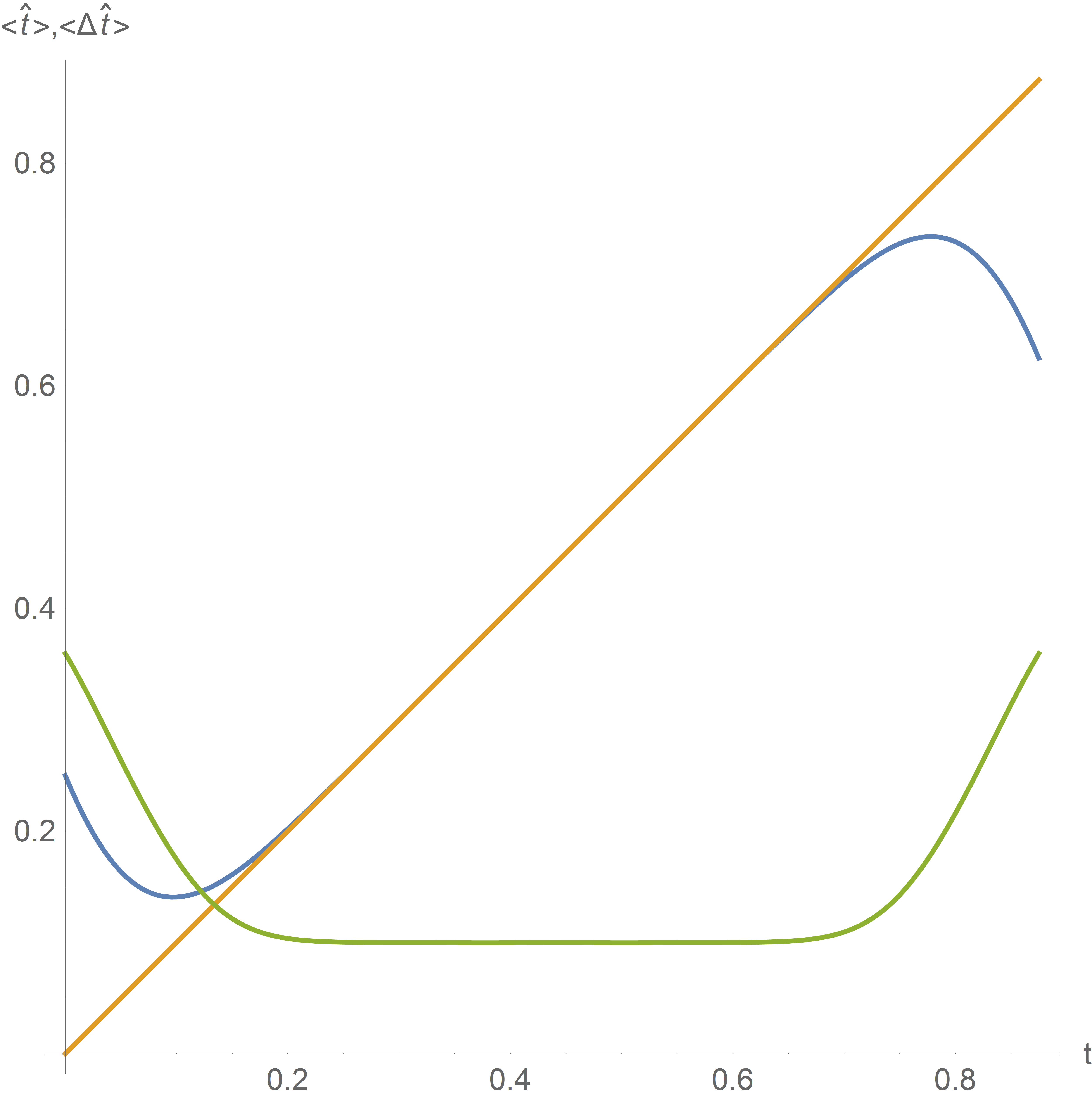
Figure 3: The expectation value (blue) and variance (green) of the time operator Eq. (14) given the initial state $\ket{\Psi(0)}\in\Lambda_{\sqrt{d},(d-1)/2}$, (referred to as symmetric, see Def. 5 and Remark VII.6) for $d=8$, $T_{0}=1$. The ideal case $\braket{\hat{t}}=t$ is in orange. If one compares this to the analogous plot for time states rather than the state used here (See Fig. 5, Section B.2 in the appendix), it is apparent that time states produce a mean and standard deviation which is much worse.

Definition 3.

(Analytic extension of clock states). Corresponding to every $\ket{\Psi(k_{0})}\in\Lambda_{\sigma,n_{0}}$, we define $\psi:{\mathbbm{R}}\rightarrow\mathbb{C}$ to be the analytic Gaussian function

$$\psi(k_{0};x)=Ae^{-\frac{\pi}{\sigma^{2}}(x-k_{0})^{2}}e^{i2\pi n_{0}(x-k_{0})/d}.$$ (29)

By definition, $\psi(k_{0};k)=\braket{\theta_{k}}{\Psi(k_{0})}$ for $k\in\mathcal{S}_{d}(k_{0})$, and thus $\psi$ is an analytic extension of the discrete coefficients $\braket{\theta_{k}}{\Psi(k_{0})}$.

In the special case that the corresponding state $\ket{\Psi(k_{0})}\in\Lambda_{\sigma,n_{0}}$ is normalised, $\psi$ will be denoted accordingly, namely

$$\psi_{\textup{nor}}(k_{0};k):=\psi(k_{0};k)\quad\text{iff }A\text{ satisfies Eq. \eqref{eq:A normalised}}$$ (30)

Remark VII.5.

$\psi(k_{0};k+y)=\psi(k_{0}-y;k)$.

Definition 4.

(Continuous Fourier Transform as a function of dimension $d$ of clock state). Let $\tilde{\psi}:{\mathbbm{R}}\rightarrow\mathbb{C}$ be defined as the continuous Fourier transform of $\psi$,

$$\tilde{\psi}(k_{0};p) =\frac{1}{\sqrt{d}}\int_{-\infty}^{\infty}\psi(k_{0};x)\mathrm{e}^{-\mathrm{i}2\pi px/d}dx=A\frac{\sigma}{\sqrt{d}}\mathrm{e}^{-\frac{\pi\sigma^{2}}{d^{2}}(p-n_{0})^{2}}\mathrm{e}^{-i2\pi nk_{0}/d}.$$ (31)

Similarly to above, we denote

$$\tilde{\psi}_{\textup{nor}}(k_{0};p):=\tilde{\psi}(k_{0};p)\quad\text{iff }A\text{ satisfies Eq. \eqref{eq:A normalised}}.$$ (32)

Lemma VII.0.1 (The clock state in the energy basis).

This Lemma states that the continuous Fourier transform $\tilde{\psi}(k_{0};p)$ is an exponentially good approximation (w.r.t. dimension $d$) of the clock state in the energy basis. Mathematically this is a statement of the closeness of the discrete Fourier transform (D.F.T.) to the continuous Fourier transform (C.F.T.) for Quasi-Ideal clock states. For simplicity, we state the result for the special case $\sigma=\sqrt{d}$, $n_{0}=(d-1)/2$.

$$\left|\braket{E_{n}}{\Psi_{\textup{nor}}(k_{0})}-\tilde{\psi}_{\textup{nor}}(k_{0};n)\right|<\left(\frac{2^{\frac{9}{4}}}{1-e^{-\pi}}\right)d^{-\frac{1}{4}}e^{-\frac{\pi d}{4}},\quad n=0,1,2,\ldots,d-1.$$ (33)

Proof.

From the definition of the state, Eq. (1), and the relation between the time states and energy states Eq. (6),

$$\braket{E_{n}}{\Psi(k_{0})} =\frac{1}{\sqrt{d}}\;\;\;\sum_{k\in\mathcal{S}_{d}(k_{0})}\psi(k_{0};k)e^{-i2\pi nk/d}.$$ (34)

By definition, this is the D.F.T. of the $\psi(k_{0};k)$, state in the time basis. To prove that this approximates the C.F.T. of the state $\psi(k_{0},k)$, we first convert the finite sum above to the infinite sum $k\in\mathbb{Z}$, and bound the difference using Lemma E.0.1,

$$\left|\frac{1}{\sqrt{d}}\;\;\;\sum_{k\in\mathcal{S}(d,k_{0})}\psi_{\textup{nor}}(k_{0};k)\,e^{-i2\pi nk/d}-\frac{1}{\sqrt{d}}\;\;\;\sum_{\mathclap{\begin{subarray}{c}k\in\mathbb{Z}\end{subarray}}}\psi_{\textup{nor}}(k_{0};k)\,e^{-i2\pi nk/d}\right|<\left(\frac{2^{\frac{5}{4}}}{1-e^{-\pi}}\right)d^{-\frac{3}{4}}e^{-\frac{\pi d}{4}},$$ (35)

where we have used the bound for $A$ for normalized states derived in Section E.1.1. Applying the Poisson summation formula (Corollary C.0.2) on the infinite sum,

$$\frac{1}{\sqrt{d}}\;\;\;\sum_{k\in\mathbb{Z}}\psi_{\textup{nor}}(k_{0};k)e^{-i2\pi nk/d}=\sum_{m\in\mathbb{Z}}\tilde{\psi}_{\textup{nor}}(k_{0};n+md).$$ (36)

Using Lemma E.0.1, we can approximate the sum by the $m=0$ term,

$$\left|\tilde{\psi}_{\textup{nor}}(k_{0};n)-\sum_{m\in\mathbb{Z}}\tilde{\psi}_{\textup{nor}}(k_{0};n+md)\right|<\left(\frac{2^{\frac{5}{4}}}{1-e^{-\pi}}\right)d^{-\frac{1}{4}}e^{-\frac{\pi d}{4}}.$$ (37)

Adding the two error terms, we arrive at the Lemma statement. ∎

Remark VII.6 (Symmetry of clock states).

Now that we know the C.F.T. $\psi$ to be a good approximation of the clock state in the energy basis, we can note the two most important features. First, the width of the state in the energy basis is of the same order ($\sqrt{d}$) as that in the time basis, Eq. (29). The states are thus symmetric w.r.t. the uncertainty in either basis. In general when $\sigma\neq\sqrt{d}$, the widths of the states in the time and energy bases are of different order.

Second, the state $\ket{\Psi_{\textup{nor}}(k_{0})}$ is centered about the value $n_{0}=(d-1)/2$. Considering that the range of values for the energy number is from $0$ to $d-1$, the energy of the clock state is exactly at the middle of the spectrum. These observations motivate the following definitions.

Definition 5.

(Quasi-Ideal clock state classes) We give the following names to states $\ket{\Psi(k_{0})}\in\Lambda_{\sigma,n_{0}}$ depending on the relationship between their width $\sigma\in(0,d)$, and the clock dimension $d$:

• symmetric if $\sigma^{2}=d$.
  

• time squeezed if $\sigma^{2}<d$.
  

• energy squeezed if $\sigma^{2}>d$.

Furthermore, we add the adverb, completely when in addition $n_{0}=(d-1)/2$, i.e. $\ket{\Psi(k_{0})}\in\Lambda_{\sigma,n_{0}}$ has mean energy centered at the middle of the spectrum of $\hat{H}_{c}$.

VIII Proof of quasi-continuity of Quasi-Ideal clock states

Recall the continuity of the idealized clock, Eq. (3). The time-translated state of the clock was the same as the space-translated state, for arbitrary translation size. Our first major result is to derive an analogous statement for the finite clock. This is the subject of this section, with the Theorem stated at the end (Theorem VIII.1).

Sketch of proof:

The mean position $k_{0}$ of the clock state appears twice in the expression for the state, first as the mean of the Gaussian $\psi(k_{0};k)$, and second as determining the set of integers $k$ over which the time states $\ket{\theta_{k}}$ are defined.

Therefore, in order to prove that time translations are (approximately) equivalent to translations in position, we prove that an arbitrary time translation of the clock by a value $\Delta$ shifts both $k_{0}$ to $k_{0}+\Delta$ and the set $\mathcal{S}(k_{0})$ to $\mathcal{S}(k_{0}+\Delta)$.

By the properties of $\mathcal{S}(k_{0})$, we see that it changes at definite values of $k_{0}$ (integer values if $d$ is even, and half-integer values if $d$ is odd).

We proceed in a number of steps. First we prove that an infinitesimal time translation by $\delta$ is approximately equivalent to shifting only the mean $k_{0}$ by $\delta$. We then use the Lie-Product formula to extend the statement to finite time-translations of $\Delta$ that are small enough so that $\mathcal{S}(k_{0}+\Delta)$ is the same as $\mathcal{S}(k_{0})$.

We then bound the error involved in switching the set $\mathcal{S}(k_{0})$ to $\mathcal{S}(k_{0}+1)$ (without any other change in the state).

Together the two results then provide a manner of calculating the state for arbitrary time translations: first move only the mean $k_{0}$ for one unit, then switch $\mathcal{S}(k_{0})$ by one integer, and repeat.

We proceed by deriving all the necessary technical lemmas which are necessary for Theorem VIII.1. We first prove the quasi-continuity of the Quasi-Ideal clock states under infinitesimal time-translations, followed by extending the proof to arbitrary times.

Lemma VIII.0.1.

The action of the clock Hamiltonian on a Quasi-Ideal clock state for infinitesimal time of order $\delta$ may be approximated by an infinitesimal translation of the same order on the analytic extension of the clock state. Precisely speaking, for $\ket{\Psi(k_{0})}\in\Lambda_{\sigma,n_{0}}$,

$$e^{-i\delta\frac{T_{0}}{d}\hat{H}_{c}}\ket{\Psi(k_{0})}=e^{-i\delta\frac{T_{0}}{d}\hat{H}_{c}}\sum_{k\in\mathcal{S}_{d}(k_{0})}\psi(k_{0};k)\ket{\theta_{k}}=\sum_{k\in\mathcal{S}_{d}(k_{0})}\psi(k_{0}+\delta;k)\ket{\theta_{k}}+\ket{\epsilon},$$ (38)

where the $l_{2}$ norm of the error $\ket{\epsilon}$ is bounded by

$$\left|\!\left|\ket{\epsilon}\right|\!\right|_{2} \leq\delta\epsilon_{total}+\delta^{2}C^{\prime},\quad\text{where $C^{\prime}$ is $\delta$ independent, and }$$ (39)

$$\frac{\epsilon_{total}}{2\pi Ad} <\begin{cases}\displaystyle\left(2\sqrt{d}\left(\frac{1}{2}+\frac{1}{2\pi d}+\frac{1}{1-e^{-\pi}}\right)e^{-\frac{\pi d}{4}}+\frac{2}{1-e^{-\pi}}+\frac{1}{2}+\frac{1}{2\pi d}\right)e^{-\frac{\pi d}{4}}&\mbox{if }\sigma=\sqrt{d}\\[10.0pt] \displaystyle\left(2\sigma\left(\frac{\alpha_{0}}{2}+\frac{1}{2\pi\sigma^{2}}+\frac{1}{1-e^{-\pi\sigma^{2}\alpha_{0}}}\right)e^{-\frac{\pi\sigma^{2}}{4}\alpha_{0}^{2}}+\left(\frac{1}{1-e^{-\frac{\pi d}{\sigma^{2}}}}+\frac{1}{1-e^{-\frac{\pi d^{2}}{\sigma^{2}}}}+\frac{d}{2\sigma^{2}}+\frac{1}{2\pi d}\right)e^{-\frac{\pi d^{2}}{4\sigma^{2}}}\right)&\mbox{otherwise}\end{cases}$$ (40)

Remark VIII.1.

Before we begin the proof, note that the R.H.S. of Eq. (38) is not necessarily $\ket{\Psi(k_{0}+\delta)}$, since the summation is still over the set of integers $\mathcal{S}_{d}(k_{0})$, and not $\mathcal{S}_{d}(k_{0}+\delta)$ which may be different, see Eq. (22) and the remark VII.3 that follows.

Proof.

$$e^{-i\delta\frac{T_{0}}{d}\hat{H}_{c}}\ket{\Psi(k_{0})} =e^{-i\delta\frac{T_{0}}{d}\sum_{m=0}^{d-1}\frac{2\pi}{T_{0}}m\ket{E_{m}}\bra{E_{m}}}\sum_{k\in\mathcal{S}_{d}(k_{0})}\psi(k_{0};k)\ket{\theta_{k}}.$$ (41)

Switching to the basis of energy states so as to apply the Hamiltonian, and back to the basis of time states, via Eq. (6),

$$e^{-i\delta\frac{T_{0}}{d}\hat{H}_{c}}\ket{\Psi(k_{0})} =\sum_{k,l\in\mathcal{S}_{d}(k_{0})}\psi(k_{0},k)\left(\frac{1}{d}\sum_{n=0}^{d-1}e^{-i2\pi n(k+\delta-l)/d}\right)\ket{\theta_{l}}$$ (42)

We label the coefficient in the time basis of the exact state and the approximation as

$$c_{l}(\delta) =\braket{\theta_{l}}{e^{-i\delta\frac{T_{0}}{d}\hat{H}_{c}}}{\Psi(k_{0})}=\sum_{k\in\mathcal{S}_{d}(k_{0})}\psi(k_{0},k)\left(\frac{1}{d}\sum_{n=0}^{d-1}e^{-i2\pi n(k+\delta-l)/d}\right),$$ (43)

$$c^{\prime}_{l}(\delta) =\bra{\theta_{l}}\sum_{k\in\mathcal{S}_{d}(k_{0})}\psi(k_{0}+\delta;k)\ket{\theta_{k}}=\psi\left(k_{0}+\delta;l\right).$$ (44)

By the properties of the analytic extension $\psi$, both of the above are analytic functions w.r.t. $\delta$, and we can express the difference between the coefficients via the Taylor series expansion about $\delta=0$,

$$c_{l}(\delta)-c^{\prime}_{l}(\delta) =c_{l}(0)-c^{\prime}_{l}(0)+\delta\left[\frac{\partial c_{l}(\delta)}{\partial\delta}-\frac{\partial c^{\prime}_{l}(\delta)}{\partial\delta}\right]\bigg{|}_{\delta=0}+C\delta^{2},$$ (45)

$$\text{where }C =\frac{1}{2}\left(\text{max}_{|t|\leq\delta}\left|\frac{\partial^{2}c_{l}(t)}{\partial t^{2}}-\frac{\partial^{2}c^{\prime}_{l}(t)}{\partial t^{2}}\right|\right).$$ (46)

$C$ is upper bounded by a $\delta$ independent constant because the second derivatives w.r.t. $\delta$ of both $c_{l}(\delta)$ and $c^{\prime}_{l}(\delta)$ can be verified to be finite sums of bounded quantities, and therefore bounded.

We now simplify Eq. (45). By direct substitution, $c_{l}(0)=c^{\prime}_{l}(0)$. For the first derivatives,

$$\frac{\partial c_{l}(\delta)}{\partial\delta}\bigg{|}_{\delta=0} =\left[\frac{\partial}{\partial\delta}\sum_{k\in\mathcal{S}_{d}(k_{0})}\psi(k_{0};k)\left(\frac{1}{d}\sum_{n=0}^{d-1}e^{-i2\pi n(k+\delta-l)/d}\right)\right]_{\delta=0}$$ (47)

$$=\left(\frac{-i2\pi}{d^{2}}\right)\sum_{k\in\mathcal{S}_{d}(k_{0})}\psi(k_{0};k)\sum_{n=0}^{d-1}ne^{-i2\pi n(k-l)/d}$$ (48)

One can replace the finite sum over $k$ by an infinite sum, and bound the difference via Lemma E.0.1,

$$\frac{\partial c_{l}(\delta)}{\partial\delta}\bigg{|}_{\delta=0} =\left(\frac{-i2\pi}{d^{2}}\right)\sum_{k\in\mathbb{Z}}\psi(k_{0};k)e^{-i2\pi nk/d}\sum_{n=0}^{d-1}ne^{i2\pi nl/d}+\epsilon_{1},$$ (49)

$$\text{where}\;\;\;\;\;\left|\epsilon_{1}\right| <\begin{cases}\displaystyle 2\pi A\frac{e^{-\frac{\pi d}{4}}}{1-e^{-\pi}}&\mbox{if }\sigma=\sqrt{d}\\[5.0pt] \displaystyle 2\pi A\frac{e^{-\frac{\pi d^{2}}{4\sigma^{2}}}}{1-e^{-\frac{\pi d}{\sigma^{2}}}}&\mbox{otherwise}\end{cases}$$ (50)

Applying the Poisson summation formula C.0.2 upon the infinite sum,

$$\frac{\partial c_{l}(\delta)}{\partial\delta}\bigg{|}_{\delta=0} =\left(\frac{-i2\pi}{d\sqrt{d}}\right)\sum_{n=0}^{d-1}\sum_{m\in\mathbb{Z}}\tilde{\psi}(k_{0};n+md)\;ne^{i2\pi nl/d}+\epsilon_{1}$$ (51)

Since $\sum_{n=0}^{d-1}\sum_{m\in\mathbb{Z}}f(n+md)=\sum_{s\in\mathbb{Z}}f(s)$, after some arithmetic manipulation,

$$\frac{\partial c_{l}(\delta)}{\partial\delta}\bigg{|}_{\delta=0} =\left(\frac{-i2\pi}{d\sqrt{d}}\right)\left(\sum_{s\in\mathbb{Z}}\tilde{\psi}(k_{0};s)\;se^{i2\pi sl/d}-\sum_{n=0}^{d-1}\sum_{m=-\infty}^{\infty}\tilde{\psi}(k_{0};n+md)\;mde^{i2\pi nl/d}\right)+\epsilon_{1}$$ (52)

The second summation is a small contribution and may be bound in a similar way to $\epsilon_{1}$, via Lemmas E.0.1-E.0.2. Therefore,

$$\frac{\partial c_{l}(\delta)}{\partial\delta}\bigg{|}_{\delta=0} =\left(\frac{-i2\pi}{d\sqrt{d}}\right)\sum_{s\in\mathbb{Z}}\tilde{\psi}(k_{0};s)\;se^{i2\pi sl/d}+\epsilon_{2}+\epsilon_{1},$$ (53)

where (54)

$$\left|\epsilon_{2}\right| <\begin{cases}\displaystyle 4\pi A\sqrt{d}\left(\frac{1}{2}+\frac{1}{2\pi d}+\frac{1}{1-e^{-\pi d}}\right)e^{-\frac{\pi d}{4}}&\mbox{if }\sigma=\sqrt{d}\\[10.0pt] \displaystyle 4\pi A\sigma\left(\frac{\alpha_{0}}{2}+\frac{1}{2\pi\sigma^{2}}+\frac{1}{1-e^{-\pi\sigma^{2}\alpha_{0}}}\right)e^{-\frac{\pi\sigma^{2}}{4}\alpha_{0}^{2}}&\mbox{otherwise}\end{cases}$$ (55)

Apply the Poisson summation on the remaining sum, Corollaries C.0.2,

$$\frac{\partial c_{l}(\delta)}{\partial\delta}\bigg{|}_{\delta=0} =\left(\frac{-i2\pi}{d\sqrt{d}}\right)\sqrt{d}\left(\frac{-id}{2\pi}\right)\sum_{m\in\mathbb{Z}}\frac{\partial}{\partial x}\psi\left(k_{0};x+l\right)\bigg{|}_{x=md}+\epsilon_{2}+\epsilon_{1}$$ (56)

Substituting $y=-x$, and using $\psi(k_{0};l-y)=\psi(k_{0}+y,l)$, VII.5,

$$\frac{\partial c_{l}(\delta)}{\partial\delta} =\sum_{m\in\mathbb{Z}}\frac{\partial}{\partial y}\psi(k_{0}+y;l)\bigg{|}_{y=md}+\epsilon_{2}+\epsilon_{1}.$$ (57)

The $m=0$ term in the sum above is exactly the derivative $\partial c_{l}^{\prime}(\delta)/\partial\delta$ given by Eq. (44). We may bound the remainder of the sum using Lemmas E.0.1-E.0.2,

$$\frac{\partial c_{l}(\delta)}{\partial\delta} =\frac{\partial c_{l}^{\prime}(\delta)}{\partial\delta}+\epsilon_{3}+\epsilon_{2}+\epsilon_{1}$$ (58)

$$\text{where}\;\;\;\;\;\left|\epsilon_{3}\right| <\begin{cases}\displaystyle 4\pi A\left(\frac{1}{2}+\frac{1}{2\pi d}+\frac{1}{1-e^{-\pi}}\right)e^{-\frac{\pi d}{4}}&\mbox{if }\sigma=\sqrt{d}\\[10.0pt] \displaystyle 4\pi A\left(\frac{d}{2\sigma^{2}}+\frac{1}{2\pi d}+\frac{1}{1-e^{-\frac{\pi d^{2}}{\sigma^{2}}}}\right)e^{-\frac{\pi d^{2}}{4\sigma^{2}}}&\mbox{otherwise}\end{cases}$$ (59)

The Taylor series expansion Eq. (45) thus ends up as

$$c_{l}(\delta)-c^{\prime}_{l}(\delta) =\delta(\epsilon_{1}+\epsilon_{2}+\epsilon_{3})+C\delta^{2},$$ (60)

where using Eqs. (50),(54),(59), the sum of the errors is bounded by $\left|\epsilon_{1}+\epsilon_{2}+\epsilon_{3}\right|\leq\epsilon_{4}$,

$$\epsilon_{4}<\begin{cases}\displaystyle 2\pi A\left(2\sqrt{d}\left(\frac{1}{2}+\frac{1}{2\pi d}+\frac{1}{1-e^{-\pi}}\right)e^{-\frac{\pi d}{4}}+\frac{2}{1-e^{-\pi}}+\frac{1}{2}+\frac{1}{2\pi d}\right)e^{-\frac{\pi d}{4}}&\mbox{if }\sigma=\sqrt{d}\\[10.0pt] \displaystyle 2\pi A\Bigg{(}2\sigma\left(\frac{\alpha_{0}}{2}+\frac{1}{2\pi\sigma^{2}}+\frac{1}{1-e^{-\pi\sigma^{2}\alpha_{0}}}\right)e^{-\frac{\pi\sigma^{2}}{4}\alpha_{0}^{2}}\\ \quad\quad\quad\quad\quad\quad\quad\quad\quad\quad\quad\quad\quad+\left(\frac{1}{1-e^{-\frac{\pi d}{\sigma^{2}}}}+\frac{1}{1-e^{-\frac{\pi d^{2}}{\sigma^{2}}}}+\frac{d}{2\sigma^{2}}+\frac{1}{2\pi d}\right)e^{-\frac{\pi d^{2}}{4\sigma^{2}}}\Bigg{)}&\mbox{otherwise}\end{cases}$$ (61)

Note that $\epsilon_{total}$ is independent of the index $l$. Reconstructing the ideal and approximate states from the coefficients $c_{l}$ and $c_{l}^{\prime}$, we arrive at the error in the state,

$$\left|\!\left|\ket{\epsilon}\right|\!\right|_{2}\leq\sum_{l\in\mathcal{S}_{d}(k_{0})}\left|c_{l}(\delta)-c_{l}^{\prime}(\delta)\right|\leq\delta d\epsilon_{4}+dC\delta^{2}.$$ (62)

∎

Lemma VIII.0.2 (Finite time translations within a single time step).

Given an initial mean position $k_{0}$ and a translation of $\Delta$, s.t. $\mathcal{S}_{d}(k_{0})=\mathcal{S}_{d}(k_{0}+\Delta)$, then

$$e^{-i\frac{T_{0}}{d}\Delta\hat{H}_{c}}\ket{\Psi(k_{0})}=\ket{\Psi(k_{0}+\Delta)}+\ket{\epsilon},\text{ where }\left|\!\left|\ket{\epsilon}\right|\!\right|_{2}<\Delta\epsilon_{total},$$ (63)

where $\epsilon_{total}$ is defined in Eq. (40).

Proof.

Split the translation $\Delta$ into $M$ equal steps. Then from Lemma VIII.0.1, for $n\in\{0,1,...,M-1\}$,

$$e^{-i\frac{T_{0}}{d}\frac{\Delta}{M}\hat{H}_{c}}\ket{\Psi(k_{0}+n\Delta/M)}=\ket{\Psi(k_{0}+(n+1)\Delta/M)}+\ket{\epsilon},\text{ where }\left|\!\left|\ket{\epsilon}\right|\!\right|_{2}<\frac{\Delta}{M}\epsilon_{total}+C^{\prime}\frac{\Delta^{2}}{M^{2}}.$$ (64)

Applying Lemma C.0.2, when we add all the steps, we obtain,

$$\left|\!\left|\ket{\Psi(k_{0}+\Delta)}-\left(e^{-i\frac{T_{0}}{d}\frac{\Delta}{M}\hat{H}_{c}}\right)^{M}\ket{\Psi(k_{0})}\right|\!\right|_{2}<M\left(\frac{\Delta}{M}\epsilon_{total}+C^{\prime}\frac{\Delta^{2}}{M^{2}}\right).$$ (65)

Therefore,

$$\left|\!\left|\ket{\Psi(k_{0}+\Delta)}-e^{-i\frac{T_{0}}{d}\Delta\hat{H}_{c}}\ket{\Psi(k_{0})}\right|\!\right|_{2}<\Delta\epsilon_{total}+C^{\prime}\frac{\Delta^{2}}{M}.$$ (66)

We are free to choose any positive integer $M$, so we take the limit $M\rightarrow\infty$, which recovers the statement of the Lemma. ∎

At this point, we have already proven the continuity of the clock state for time translations that are finite, but small (i.e. small enough that the range $\mathcal{S}_{d}(k_{0})$ remains the same). In order to generalize the statement to arbitrary translations we need to be able to shift the range itself, which is the goal of the following Lemma.

Lemma VIII.0.3 (Shifting the range of the clock state).

If $d$ is even, and the mean of the clock state $k_{0}$ is an integer, or alternatively, if $d$ is $odd$ and $k_{0}$ is a half integer, then

$$\left|\!\left|\sum_{k\in\mathcal{S}_{d}(k_{0}-1)}\psi(k_{0};k)\ket{\theta_{k}}-\sum_{k\in\mathcal{S}_{d}(k_{0})}\psi(k_{0};k)\ket{\theta_{k}}\right|\!\right|_{2} <\epsilon_{step},$$ (67)

$$\text{where}\quad\left|\epsilon_{step}\right| <\begin{cases}\displaystyle 2Ae^{-\frac{\pi d}{4}}&\mbox{if }\sigma=\sqrt{d}\\[10.0pt] \displaystyle 2Ae^{-\frac{\pi d^{2}}{4\sigma^{2}}}&\mbox{otherwise}\end{cases}$$ (68)

Proof.

We prove the statement for even $d$, the proof for odd $d$ is analogous.

By definition (see Eq. (22)), $\mathcal{S}_{d}(k_{0})$ is a set of $d$ consecutive integers. Thus the only difference between $\mathcal{S}_{d}(k_{0})$ and $\mathcal{S}_{d}(k_{0}-1)$ is the leftmost integer of $\mathcal{S}_{d}(k_{0}-1)$ and the rightmost integer of $\mathcal{S}_{d}(k_{0})$, which differ by precisely $d$. By direct calculation, these correspond to the integers $k_{0}-d/2$ and $k_{0}+d/2$. These are the only two terms that do not cancel out in the statement of the Lemma,

$$\left|\!\left|\sum_{k\in\mathcal{S}_{d}(k_{0}-1)}\psi(k_{0};k_{0})\ket{\theta_{k}}-\sum_{k\in\mathcal{S}_{d}(k_{0})}\psi(k_{0};k)\ket{\theta_{k}}\right|\!\right|_{2}=\left|\!\left|\psi(k_{0};k_{0}-d/2)\ket{\theta_{k_{0}-d/2}}-\psi(k_{0};k_{0}+d/2)\ket{\theta_{k_{0}+d/2}}\right|\!\right|_{2}.$$ (69)

But $\ket{\theta_{k_{0}-d/2}}=\ket{\theta_{k_{0}+d/2}}$,

$$\left|\!\left|\sum_{k\in\mathcal{S}_{d}(k_{0}-1)}\psi(k_{0};k_{0})\ket{\theta_{k}}-\sum_{k\in\mathcal{S}_{d}(k_{0})}\psi(k_{0};k)\ket{\theta_{k}}\right|\!\right|_{2}=\left|\psi(k_{0};k_{0}-d/2)-\psi(k_{0};k_{0}+d/2)\right|.$$ (70)

By direct substitution of $\psi(k_{0};k_{0}-d/2)$ and $\psi(k_{0};k_{0}+d/2)$ from Eq. (29), we arrive at the Lemma statement. ∎

Theorem VIII.1 (Quasi-continuity of Quasi-Ideal clock states).

Let $k_{0},t\in{\mathbbm{R}}$. Then the effect of the Hamiltonian $\hat{H}_{c}$ for the time $t$ on $\ket{{\Psi}_{\textup{nor}}(k_{0})}\in\Lambda_{\sigma,n_{0}}$ is approximated by

$$\mathrm{e}^{-\mathrm{i}t\hat{H}_{c}}\ket{\Psi_{\textup{nor}}(k_{0})}=\ket{\Psi_{\textup{nor}}(k_{0}+t\frac{d}{T_{0}})}+\ket{\epsilon},$$ (71)

where in the limits $d\rightarrow\infty$, $(0,d)\ni\sigma\rightarrow\infty$,

$$\varepsilon_{c}:=\left|\!\left|\ket{\epsilon}\right|\!\right|_{2}=\begin{cases}\displaystyle\frac{|t|}{T_{0}}\,\mathcal{O}\left(d^{9/4}\right)\mathrm{e}^{-\frac{\pi}{4}d\alpha_{0}^{2}}+\mathcal{O}\left(d^{-1/4}\right)\mathrm{e}^{-\frac{\pi}{4}d}&\mbox{if }\sigma=\sqrt{d}\\[10.0pt] \displaystyle\frac{|t|}{T_{0}}\left(\mathcal{O}\left(d^{2}\sigma^{1/2}\right)\mathrm{e}^{-\frac{\pi}{4}\sigma^{2}\alpha_{0}^{2}}+\mathcal{O}\left(1+\frac{d^{3}}{\sigma^{3/4}}\right)\mathrm{e}^{-\frac{\pi}{4}\frac{d^{2}}{\sigma^{2}}}\right)+\mathcal{O}\left(\mathrm{e}^{-\frac{\pi}{4}\frac{d^{2}}{\sigma^{2}}}\right)+\mathcal{O}\left(\mathrm{e}^{-\frac{\pi}{4}\sigma^{2}}\right)&\mbox{otherwise}\end{cases}$$ (72)

More precisely,

$$\varepsilon_{c}=\left|\!\left|\ket{\epsilon}\right|\!\right|_{2} <|t|\frac{d}{T_{0}}\epsilon_{total}+\left(|t|\frac{d}{T_{0}}+1\right)\epsilon_{step}+\epsilon_{\textup{nor}}(t),$$ (73)

where,

$$\epsilon_{total}=\!\begin{cases}\displaystyle 2\pi Ad\left(2\sqrt{d}\left(\frac{\alpha_{0}}{2}+\frac{1}{2\pi d}+\frac{1}{1-e^{-\pi\alpha_{0}}}\right)e^{-\frac{\pi d}{4}\alpha_{0}^{2}}+\left(\frac{2}{1-e^{-\pi}}+\frac{1}{2}+\frac{1}{2\pi d}\right)e^{-\frac{\pi d}{4}}\right)\!&\mbox{if }\sigma=\sqrt{d}\\[10.0pt] 2\pi Ad\left(2\sigma\left(\frac{\alpha_{0}}{2}+\frac{1}{2\pi\sigma^{2}}+\frac{1}{1-e^{-\pi\sigma^{2}\alpha_{0}}}\right)e^{-\frac{\pi\sigma^{2}}{4}\alpha_{0}^{2}}+\left(\frac{1}{1-e^{-\frac{\pi d}{\sigma^{2}}}}+\frac{1}{1-e^{-\frac{\pi d^{2}}{\sigma^{2}}}}+\frac{d}{2\sigma^{2}}+\frac{1}{2\pi d}\right)e^{-\frac{\pi d^{2}}{4\sigma^{2}}}\right)\!&\mbox{otherwise},\end{cases}$$ (74)

with $A=\mathcal{O}(\sigma^{-1/2})$ and is upper bounded by Eq. (483), and

$$\epsilon_{step} <\begin{cases}2Ae^{-\frac{\pi d}{4}}&\mbox{if }\sigma=\sqrt{d}\\ 2Ae^{-\frac{\pi d^{2}}{4\sigma^{2}}}&\mbox{otherwise.}\end{cases}$$ (75)

$$\epsilon_{\textup{nor}}(t) =\left|\sqrt{\frac{\sum_{k\in\mathcal{S}_{d}(k_{0}+td/T_{0})}\mathrm{e}^{-\frac{2\pi}{\sigma^{2}}(k-k_{0}-\frac{d}{T_{0}}t)^{2}}}{\sum_{l\in\mathcal{S}_{d}(k_{0})}\mathrm{e}^{-\frac{2\pi}{\sigma^{2}}(l-k_{0})^{2}}}}-1\right|\leq\begin{cases}\displaystyle\frac{40}{3}\frac{\mathrm{e}^{-\frac{\pi}{2}d}}{1-\mathrm{e}^{-\pi}}\quad&\forall\,t\in{\mathbbm{R}}\;\;\mbox{ if }\sigma=\sqrt{d}\\[10.0pt] \displaystyle\frac{40\sqrt{2}}{3\sigma}\left(\frac{\mathrm{e}^{-\frac{\pi d^{2}}{2\sigma^{2}}}}{1-\mathrm{e}^{-\frac{2\pi d}{\sigma^{2}}}}+\frac{\sigma}{\sqrt{2}}\frac{\mathrm{e}^{-\frac{\pi\sigma^{2}}{2}}}{1-\mathrm{e}^{-\pi\sigma^{2}}}\right)\quad&\forall\,t\in{\mathbbm{R}}\;\;\mbox{ otherwise},\end{cases}$$ (76)

where on the r.h.s. of the inequality in Eq. (76) we have assumed $\sigma\geq 1$, $d=2,3,4,\ldots$; (tighter bounds can be found in Section E.1.2).

Intuition. The discrete clock mimics the perfect clock, with an error that grows linearly with time, and scales better than any inverse polynomial w.r.t. the dimension of the clock. The optimal decay is when the state is completely symmetric, (see Def. 5). This gives exponentially small error in $d$, the clock dimension, with a decay rate coefficient $\pi/4$. When the initial clock state is symmetric, but not completely symmetric, the error is still exponential decay but now with a modified coefficient which decreases as the clock’s initial state’s mean energy approaches either end of the spectrum of $\hat{H}_{c}$.

Proof.

For, $t\geq 0$, directly apply the previous two Lemmas (VIII.0.2, VIII.0.3) in alternation, first to move $k_{0}$ from one integer to the next, then to switch from ${\lfloor k_{0}\rfloor}$ to ${\lfloor k_{0}+1\rfloor}$ if $d$ is even, and ${\lfloor k_{0}+1/2\rfloor}$ to ${\lfloor k_{0}+1/2+1\rfloor}$ if $d$ is odd, and finally arriving at

$$\mathrm{e}^{-it\hat{H}_{c}}\ket{{\Psi}(k_{0})} =\ket{{\Psi}(k_{0}+\frac{d}{T_{0}}t)}+\ket{\epsilon},\quad\quad\left|\!\left|\ket{\epsilon}\right|\!\right|_{2}\leq t\frac{d}{T_{0}}\epsilon_{total}+\left(t\frac{d}{T_{0}}+1\right)\epsilon_{step}.$$ (77)

To conclude Eq. (73) for $t>0$, one now has to normalize the states using bounds from Section E.1.2 and then use Lemma C.0.2 to upper bound the total error. For $t<0$, simply evaluate Eq. (71) for a time $|t|$ followed by multiplying both sides of the equation by $\exp(\mathrm{i}t\hat{H}_{c})$, mapping $k_{0}\rightarrow k_{0}-t\;d/T_{0}$ and noting the unitary invariance of the $l_{2}$ norm of $\ket{\epsilon}$. ∎

IX Autonomous quasi-control of Quasi-Ideal clock states

IX.1 Theorem and proof of autonomous quasi-control

Recall the control of the idealized clock, Eq. (4) (or Eq. 439 in Appendix for more details). Namely, the time translated state of the clock under its natural Hamiltonian plus a potential for a time $t$, was the same as the space-translated state multiplied by a phase factor, with the phase given by the integral over the potential up to time $t$. Our second major result is to derive an analogous statement for the finite clock. This is the subject of this Section, with the result in the form of a Theorem stated at the end of the Section, Theorem (IX.1). The proof will follow similar lines to the proof of the continuity of the Quasi-Ideal clock states of the previous Section (VIII). The main extra complications will be two:

• Unlike in the previous Section (VIII), the Hamiltonian will now include a potential term, i.e. $\hat{H}=\hat{H}_{c}+\hat{V}_{d}$ where $\hat{H}_{c}$ and $\hat{V}_{d}$ do not commute. To get around this difficulty, we will have to employ the Lie product formula to split the time evolution into consecutive infinitesimal time steps with separate contributions from $\hat{H}_{c}$ and $\hat{V}_{d}$. Bounding the infinitesimal time step contribution from $\hat{H}_{c}$ will be the subject of Lemma IX.0.2, while the contribution from $\hat{V}_{d}$ will be bounded in Lemma IX.0.3. Combining both contributions will be the subject of Lemma IX.0.4.

• The Fourier Transform of the clock state (see Def. 4), will be replaced by the Fourier Transform of the clock state multiplied by an exponentiated integral over the potential. Unlike in the previous case, one will not be able to perform the Fourier Transform analytically, thus requiring to upper bound how quickly it decays with clock dimension $d$. This turns out not to be so simple, and is the subject of Lemma IX.0.1 which is the main mathematically challenging difference between this section and Section VIII.

Definition 6.

(Continuous Interaction Potential). Let ${V}_{0}:{\mathbbm{R}}\rightarrow{\mathbbm{R}}\cup{\mathbbm{H}}^{-}$ (where ${\mathbbm{H}}^{-}:=\{a_{0}+\mathrm{i}b_{0}:a_{0}\in{\mathbbm{R}},b_{0}<0\}$ denotes the lower-half complex plane) be an infinitely differentiable function of period $2\pi$, normalized so that

$$\int_{x}^{x+2\pi}{V}_{0}(x^{\prime})dx^{\prime}=:\Omega\in{\mathbbm{R}}\cup{\mathbbm{H}}^{-},$$ (78)

and define ${V}_{d}:{\mathbbm{R}}\rightarrow{\mathbbm{R}}\cup{\mathbbm{H}}^{-}$ as

$${V}_{d}(x)=\frac{2\pi}{d}\,{V}_{0}\left(\frac{2\pi x}{d}\right).$$ (79)

For convenience of notation, we also define the function

$$\Theta(\Delta;x)=\int_{x-\Delta}^{x}dyV_{d}(y).$$ (80)

Definition 7.

(Interaction Potential). Let $\hat{V}_{d}$ be an operator on $\mathcal{H}_{c}$ defined by

$$\hat{V}_{d}=\frac{d}{T_{0}}\sum_{k}{V}_{d}(k)\ket{\theta_{k}}\!\!\bra{\theta_{k}}.$$ (81)

Remark IX.1.

Thus ${V}_{d}(x)$ is a continuous extension of the discrete elements $\braket{\theta_{k}}{\hat{V}_{d}}{\theta_{k}}T_{0}/d$. Note that because ${V}_{d}$ has a period of $d$, the summation in the above expression may run over any sequence of $d$ consecutive integers without affecting the operator $\hat{V}_{d}$. Note that for the special case $V_{0}:{\mathbbm{R}}\rightarrow{\mathbbm{R}}$, $\hat{V}_{d}$ is self adjoint. This is the most important case for this manuscript, and the more general case will only be useful for future work RMRenatoetal .

Definition 8.

(Decay rate parametres). Let $b$ be any real number satisfying

$$b\geq\;\sup_{k\in{\mathbbm{N}}^{+}}\left(2\max_{x\in[0,2\pi]}\left|V_{0}^{(k-1)}(x)\right|\,\right)^{1/k},$$ (82)

where $V_{0}^{(p)}(x)$ is the $p^{\textup{th}}$ derivative with respect to $x$ of $V_{0}(x)$ and $V_{0}^{(0)}:=V_{0}$. We can use $b$ to define $\mathcal{N}\in{\mathbbm{N}}^{0}$ as follows

$$\mathcal{N}=\begin{cases}\displaystyle\left\lfloor\frac{\pi\alpha_{0}^{2}}{2\left(\frac{\pi\kappa\alpha_{0}}{\ln(\pi\alpha_{0}d)}b+1\right)^{2}}\,d\right\rfloor,&\mbox{if }\sigma=\sqrt{d}\\[20.0pt] \displaystyle\left\lfloor\frac{\pi\alpha_{0}^{2}}{2\left(\frac{\pi\kappa\alpha_{0}}{\ln(\pi\alpha_{0}\sigma^{2})}b+\frac{d}{\sigma^{2}}\right)^{2}}\left(\frac{d}{\sigma}\right)^{2}\right\rfloor,&\mbox{otherwise}\end{cases}$$ (83)

where $\kappa=0.792$ and $\alpha_{0}\in(0,1)$ characterizes how close the mean energy of the initial state of the clock is to either extremum of the energy spectrum, defined in Def. 2.

We can use the above definitions to define the following parametre.

Definition 9.

(Exponential decay rate parameter). We define the rate parameter as

$$\bar{\upsilon}=\frac{\pi\alpha_{0}\kappa}{\ln\left(\pi\alpha_{0}\sigma^{2}\right)}b$$ (84)

where recall $\kappa=0.792$.

We will often require that $\bar{\upsilon}\geq 0$. This is equivalent to requiring $\pi\alpha_{0}\sigma^{2}>1$ if $b>0$, and is always satisfied in the special case $b=0$.

To proceed further, we will need a generalized definition of Def. 3 which incorporates a potential.

Definition 10.

(Continuous Fourier Transform of the control analytic extension) Let $\tilde{\psi}(k_{0};\cdot):{\mathbbm{R}}\rightarrow\mathbb{C}$ be defined as the continuous Fourier transform of $\psi$ multiplied by an exponentiated integral over the potential function,

$$\tilde{\psi}(k_{0},\Delta;p) =\frac{1}{\sqrt{d}}\int_{-\infty}^{\infty}\psi(k_{0};x)\,\mathrm{e}^{-\mathrm{i}\int_{x-\Delta}^{x}V_{d}(x^{\prime})dx^{\prime}}\mathrm{e}^{-\mathrm{i}2\pi px/d}dx,$$ (85)

where $\psi$ is defined in Def. 3 and $V_{d}$ in Def. 6.

Remark IX.2.

Note that Eq. (85) is well defined since $|\tilde{\psi}(k_{0},\Delta;p)|\leq\int_{-\infty}^{\infty}|\psi(k_{0};x)|dx/\sqrt{d}<\infty$.

Lemma IX.0.1.

(Bounding a sampled version of the Fourier Transform of the clock state with potential). Let $\bar{\epsilon}_{2}$ be defined by

$$\bar{\epsilon}_{2}=\frac{\mathrm{i}2\pi}{\sqrt{d}}\sum_{n=0}^{d-1}\sum_{k=-\infty}^{\infty}k\,\mathrm{e}^{\mathrm{i}2\pi nl/d}\,\tilde{\psi}(k_{0},\Delta;n+kd).$$ (86)

We have the bound

$$|\bar{\epsilon}_{2}|<\begin{cases}(2\pi)^{5/4}\sigma^{3/2}A\left(1+\frac{\pi^{2}}{8}\right)\sqrt{\frac{\mathrm{e}}{2}\frac{\alpha_{0}}{(\bar{\upsilon}\sigma^{2}/d+1)}}\exp\left(-\frac{\pi}{4}\frac{\alpha_{0}^{2}}{\left(\frac{d}{\sigma^{2}}+\bar{\upsilon}\right)^{2}}\left(\frac{d}{\sigma}\right)^{2}\right)\quad&\text{if }\mathcal{N}\geq 8\text{ and }\bar{\upsilon}\geq 0\\ \frac{3^{7/4}}{\sqrt{2\pi}\mathrm{e}}\frac{A(8+\pi^{2})}{\alpha_{0}^{3}}\left(\frac{\kappa\sqrt{6\pi}}{\ln(3)}b+\frac{d}{\sigma}\right)^{3}\left(\frac{\sigma}{d^{3}}\right)\quad&\text{otherwise}\end{cases}$$ (87)

where $b$, $\mathcal{N}$, and $\alpha_{0}$ are defined in Def. 8 while $\bar{\upsilon}$ in Def. 9.

Proof.

Outline: to bound $|\bar{\epsilon}_{2}|$, the main challenge is in bounding the Fourier transform $\tilde{\psi}(\cdot,\cdot;\cdot)$, and show that it is exponentially decaying in $d$ (for $d$ large enough such that the first if condition in Eq. (87) is satisfied). In order to achieve this, we will integrate by parts the Fourier transform $N=1,2,3,\ldots$ times followed by taking absolute values, thus generating a different bound for every $N$. We will then choose to bound the Fourier transform using a different bound (i.e. different $N$), depending of the value of $d$, i.e. $N=N(d)$. We will have to bound the derivatives produced by integrating by parts $N$ times. We will use results from combinatorics for this. The proof will make essential use of: the binomial theorem, the generalized Leibniz rule, Rodriguez formulas for Hermite polynomials, orthogonality conditions of Hermite polynomials, the Cauchy-Schwarz inequality, Fadi Bruno’s formula, Bell polynomials, Bell numbers, analytic upper bounds for Bell numbers, Sterling’s formula, and the Fundamental theorem of calculus. Also note that definitions 8 and 9 have been defined more generally in the proof. One could use these slightly more general definitions to tighten the bound in Eq. (87) for small $d$ if desired.

We have that

$$|\bar{\epsilon}_{2}|\leq\frac{2\pi}{\sqrt{d}}\sum_{n=0}^{d-1}\left(\sum_{s=-\infty}^{-1}|s\,\tilde{\psi}(k_{0},\Delta;n+sd)|+\sum_{s=1}^{\infty}|s\,\tilde{\psi}(k_{0},\Delta;n+sd)|\right),$$ (88)

where from definitions 10, 3 we have

$$\tilde{\psi}(k_{0},\Delta;p)=\frac{A}{\sqrt{d}}\int_{-\infty}^{\infty}dx\,\mathrm{e}^{-\frac{\pi}{\sigma^{2}}(x-k_{0})^{2}}\mathrm{e}^{\mathrm{i}2\pi n_{0}(x-k_{0})/d}\mathrm{e}^{-\mathrm{i}\theta(x)}\mathrm{e}^{-\mathrm{i}2\pi px/d}.$$ (89)

where we denote

$$\theta(x)=\frac{2\pi}{d}\int_{x-\Delta}^{x}dyV_{0}(2\pi y/d),$$ (90)

where $V_{0}(\cdot)$ is a smooth, periodic function with period $2\pi$ defined in Eq. (78). Performing the change of variable $z=2\pi(k_{0}-x)/d$, we find in Eq. (89)

$$\tilde{\psi}(k_{0},\Delta;p)=\frac{A}{\sqrt{d}}\frac{d}{2\pi}\mathrm{e}^{-\mathrm{i}p2\pi k_{0}/d}\int_{-\infty}^{\infty}dz\,U(z)\mathrm{e}^{\mathrm{i}(p+\gamma)z},$$ (91)

where

$$U(z):=\mathrm{e}^{-\left(\frac{d}{2\sqrt{\pi}\sigma}\right)^{2}z^{2}}\mathrm{e}^{-\mathrm{i}\tilde{\theta}(z)}\mathrm{e}^{-\mathrm{i}(n_{0}+\gamma)z},$$ (92)

with

$$\tilde{\theta}(z):=\theta\left(-\frac{dz}{2\pi}+k_{0}\right),$$ (93)

and $\gamma\in\big{(}-(d-1)/2,(d-1)/2\big{)}.$ We now integrate by parts $N$ times the integral in Eq. (91), differentiating $U(\cdot)$ once in every iteration. This requires that $U(\cdot)$ is differentiable $N$ times and since we will require $N$ to be unbounded from above, hence the requirement that $V_{0}(\cdot)$ is smooth. Taking this all into account, we have

$$\tilde{\psi}(k_{0},\Delta;p)=-\frac{A}{\sqrt{d}}\frac{d}{2\pi}\mathrm{e}^{-\mathrm{i}p2\pi k_{0}/d}\frac{1}{\big{(}-\mathrm{i}\left(p+\gamma\right)\big{)}^{N}}\int_{-\infty}^{\infty}dz\,U^{(N)}(z)\mathrm{e}^{\mathrm{i}\big{(}p+\gamma\big{)}z},\quad N\in{\mathbbm{N}}^{+},$$ (94)

where $U^{(N)}(z)$ denotes the $N^{\text{th}}$ derivative of $U(z)$ w.r.t. $z$. Thus taking absolute values, we achieve

$$\tilde{\psi}(k_{0},\Delta;p)\leq\frac{A}{\sqrt{d}}\frac{d}{2\pi}|p+\gamma|^{-N}\int_{-\infty}^{\infty}dz\,\left|U^{(N)}(z)\right|,\quad N\in{\mathbbm{N}}^{+}.$$ (95)

We now substitute Eq. (95) into Eq. (88) obtaining the upper bound

$$|\bar{\epsilon}_{2}| \leq\frac{2\pi}{\sqrt{d}}\frac{A}{\sqrt{d}}\frac{d}{2\pi}\left(\int_{-\infty}^{\infty}dz\left|U^{(N)}(z)\right|\right)\sum_{n=0}^{d-1}\sum_{s=1}^{\infty}\left(\frac{|s|}{\left|n+sd+\gamma\right|^{N}}+\frac{|s|}{\left|n-sd+\gamma\right|^{N}}\right)$$ (96)

$$\leq\left(AGd\int_{-\infty}^{\infty}dz\left|U^{(N)}(z)\right|\right)\left(\frac{d(1-|\beta|)}{2}\right)^{-N},\quad N=3,4,5,\ldots$$ (97)

where $\beta\in(-1,1)$ and

$$G:=\frac{1}{d}\sum_{n=0}^{d-1}\sum_{s=1}^{\infty}\frac{|s|}{\left(\frac{2}{d(1-|\beta|)}\right)^{N}}\left(\frac{1}{\big{|}n+sd+\gamma\big{|}^{N}}+\frac{1}{\big{|}n-sd+\gamma\big{|}^{N}}\right).$$ (98)

The rational to defining $G$ in this way, is that we will soon parametrize $\gamma$ in terms of $\beta$ such that $G$ will be upper bounded by a $d$ independent constant. We will now find this constant before proceeding to bound Eq. (96). First we will parametrize $\gamma$ is such a way that the symmetry in the summations of $G$ becomes transparent. Let $\gamma=-(d-1)/2-y_{0}$, $y_{0}\in\big{[}0,-(d-1)/2\big{)}$. Substituting into Eq. (98), we find

$$G= \frac{1}{d}\sum_{n=0}^{d-1}\sum_{s=1}^{\infty}\frac{|s|}{\left(\frac{2}{d(1-|\beta|)}\right)^{N}}\left(\frac{1}{\big{|}n+sd-(d-1)/2-y_{0}\big{|}^{N}}+\frac{1}{\big{|}n-sd-(d-1)/2-y_{0}\big{|}^{N}}\right)$$ (99)

$$= \frac{1}{d}\sum_{n=0}^{d-1}\sum_{s=1}^{\infty}\frac{|s|}{\left(\frac{2}{d(1-|\beta|)}\right)^{N}}\left(\frac{1}{\big{|}n+sd-(d-1)/2-y_{0}\big{|}^{N}}+\frac{1}{\big{|}-n-sd+(d-1)/2-y_{0}\big{|}^{N}}\right)$$ (100)

$$= \frac{1}{d}\sum_{n=0}^{d-1}\sum_{s=1}^{\infty}\frac{|s|}{\left(\frac{2}{d(1-|\beta|)}\right)^{N}}\left(\frac{1}{\big{|}n+sd-(d-1)/2-|y_{0}|\big{|}^{N}}+\frac{1}{\big{|}n+sd-(d-1)/2+|y_{0}|\big{|}^{N}}\right),$$ (101)

and thus the sum only depends on the modulus of $y_{0}$. We will now make the change of variable $y_{0}=(d-1)\beta/2$ with $\beta\in(-1,1)$ leading to

$$\gamma=-\left(\frac{d-1}{2}\right)(1+\beta),\quad\beta\in(-1,1).$$ (102)

Plugging this into Eq. (101) leads to

$$G= \frac{1}{d}\sum_{n=0}^{d-1}\sum_{s=1}^{\infty}\left(\frac{|s|}{\left|\frac{(2n+1+|\beta|)}{(1-|\beta|)d}-\frac{(1+|\beta|)-2s}{(1-|\beta|)}\right|^{N}}+\frac{|s|}{\left|\frac{(2n+1-|\beta|)}{(1-|\beta|)d}+\frac{(1-|\beta|)+2s}{(1-|\beta|)}\right|^{N}}\right)$$ (103)

$$= \frac{1}{d}\sum_{n=0}^{d-1}\left(\sum_{s=0}^{\infty}\frac{s+1}{\left(\frac{(2n+1+|\beta|)}{(1-|\beta|)d}+1+\frac{2s}{1-|\beta|}\right)^{N}}+\sum_{s=1}^{\infty}\frac{s}{\left(\frac{(2n+1-|\beta|)}{(1-|\beta|)d}+1+\frac{2s}{(1-|\beta|)}\right)^{N}}\right)$$ (104)

$$\leq \frac{1}{d}\sum_{n=0}^{d-1}\left(\sum_{s=0}^{\infty}\frac{s+1}{\left(1+2s\right)^{N}}+\sum_{s=1}^{\infty}\frac{s}{\left(1+2s\right)^{N}}\right)\leq 1+\sum_{s=0}^{\infty}\frac{1}{\left(2s+1\right)^{N-1}}$$ (105)

$$\leq 1+\sum_{s=0}^{\infty}\frac{1}{(2s+1)^{2}}=1+\frac{\pi^{2}}{8}\approx 2.234\quad\text{for }N=3,4,5,\ldots\,.$$ (106)

Our next task will be to bound $\int_{-\infty}^{\infty}dz\left|U^{(N)}(z)\right|$. We will start by dividing $U(z)$ into a product of unitaries: $U(z)=U_{1}(z)U_{2}(z)U_{3}(z)$ where

$$U_{1}(z):=\mathrm{e}^{-dz^{2}/4\pi},\quad U_{2}(z):=\mathrm{e}^{-\mathrm{i}\tilde{\theta}(z)},\quad U_{3}(z):=\mathrm{e}^{-\mathrm{i}(n_{0}+\gamma)z}.$$ (107)

We will take advantage of the distinct properties of $U_{1},U_{2},U_{3}$. We will start by using the general Leibniz rule for $n$ times differentiable functions $u$ and $v$:

$$(uv)^{(n)}=\sum_{k=0}^{n}\binom{n}{k}u^{(k)}v^{(n-k)},$$ (108)

where $\binom{n}{k}$ is the binomial coefficient we are using the standard superscript round bracket notation to indicated derivatives. We thus find

$$\int_{-\infty}^{\infty}dz\left|U^{(N)}(z)\right| =\int_{-\infty}^{\infty}dz\left|\sum_{k=0}^{N}\binom{N}{k}\left(U_{1}(z)U_{2}(z)\right)^{(k)}U_{3}^{(N-k)}(z)\right|$$ (109)

$$=\int_{-\infty}^{\infty}dz\left|\sum_{k=0}^{N}\binom{N}{k}\sum_{q=0}^{k}\binom{k}{q}U_{1}^{(q)}(z)U_{2}^{(k-q)}(z)\left(-\mathrm{i}(n_{0}+\gamma)\right)^{N-k}U_{3}(z)\right|$$ (110)

$$\leq\sum_{k=0}^{N}\binom{N}{k}\sum_{q=0}^{k}\binom{k}{q}|n_{0}+\gamma|^{N-k}\int_{-\infty}^{\infty}dz\left|U_{1}^{(q)}(z)U_{2}^{(k-q)}(z)\right|$$ (111)

We now need to relate $U_{1}^{(q)}$ to the Hermite polynomials in order to bound the integral. The Rodriguez formula for the $n^{\text{th}}$ Hermite polynomial $H_{n}(x)$ is Rodriguez

$$H_{n}(x)=(-1)^{n}\mathrm{e}^{x^{2}}\frac{d^{n}}{dx^{n}}\left(\mathrm{e}^{-x^{2}}\right),\quad n\in{\mathbbm{N}}^{0}.$$ (113)

By the change in variable $x=\frac{d}{2\sigma\sqrt{\pi}}z$ we can relate $U_{1}^{(q)}$ to the Hermite polynomials:

$$U^{(n)}_{1}(z)=\left(\frac{d}{2\sigma\sqrt{\pi}}\right)^{n}(-1)^{n}\,\mathrm{e}^{-\left(\frac{d}{2\sigma\sqrt{\pi}}\right)^{2}z^{2}}H_{n}\left(\frac{d}{2\sigma\sqrt{\pi}}z\right),\quad n\in{\mathbbm{N}}^{0}.$$ (114)

Due to the periodic nature of $V_{0}(\cdot)$, we have that $|U_{2}^{(k)}(z)|$ is bounded in $z\in{\mathbbm{R}}$ for $k\in{\mathbbm{N}}^{0}$. We can thus use the Cauchy–Schwarz inequality in conjunction with Eqs. (LABEL:eq:U_N_dev_in_terms_of_U1_U2), (114) to obtain

$$\int_{-\infty}^{\infty}dz\left|U^{(N)}(z)\right|$$ (115)

$$\leq\sum_{k=0}^{N}\binom{N}{k}\sum_{q=0}^{N}\binom{N}{q}|n_{0}+\gamma|^{N-k}\left(\frac{d}{2\sigma\sqrt{\pi}}\right)^{q}\sqrt{\int_{-\infty}^{\infty}dy\,\mathrm{e}^{-\left(\frac{d}{2\sigma\sqrt{\pi}}\right)^{2}y^{2}}\left|U_{2}^{(k-q)}(z)\right|^{2}\int_{-\infty}^{\infty}dzH_{q}^{2}\left(\frac{d}{2\sigma\sqrt{\pi}}\,z\right)\mathrm{e}^{-\left(\frac{d}{2\sigma\sqrt{\pi}}\,z\right)^{2}z^{2}}}$$ (116)

$$\leq\sum_{k=0}^{N}\binom{N}{k}\sum_{q=0}^{N}\binom{k}{q}|n_{0}+\gamma|^{N-k}\left(\frac{d}{2\sigma\sqrt{\pi}}\right)^{q-1/2}C_{k-q}\,\sqrt{\int_{-\infty}^{\infty}dy\,\mathrm{e}^{-\left(\frac{d}{2\sigma\sqrt{\pi}}\right)^{2}y^{2}}\int_{-\infty}^{\infty}dx\,H_{q}^{2}\left(x\right)\mathrm{e}^{-x^{2}}}$$ (117)

where we have defined

$$C_{k}\geq\left|U_{2}^{(k)}(z)\right|,\quad\forall z\in{\mathbbm{R}},\;\;\;k\in{\mathbbm{N}}^{0}.$$ (118)

Using the orthogonality conditions of the Hermite polynomialsRodriguez :

$$\int_{-\infty}^{\infty}dyH_{p}(y)H_{q}(y)\mathrm{e}^{-y^{2}}=\delta_{p,q}\sqrt{\pi}\,2^{q}(q!),\quad p,q\in{\mathbbm{N}}^{0}$$ (119)

Eq. (117) reduces to

$$\int_{-\infty}^{\infty}dz\left|U^{(N)}(z)\right|\leq \frac{2\sigma\pi}{d}\sum_{k=0}^{N}\binom{N}{k}|n_{0}+\gamma|^{N-k}\sum_{q}^{k}\binom{k}{q}\left(\frac{d}{\sigma\sqrt{2\pi}}\right)^{q}C_{N-q}\sqrt{(q!)}.$$ (120)

Before we can continue, we will now bound $C_{k}$ in terms of derivatives of $\tilde{\theta}(\cdot)$. For this, let us first recall Faà di Bruno’s formula written in terms of the Incomplete Bell Polynomials $B_{n,k}(x_{1},x_{2},\ldots,x_{n-k+1})$ Faa_di_Bruno : for $u$,$v$ $n$-times differentiable functions, we have

$$\frac{d^{n}}{dx^{n}}u\left(v(x)\right)=\sum_{k=0}^{n}u^{(k)}\left(v(x)\right)B_{n,k}\left(v^{(1)}(x),v^{(2)}(x),\ldots,v^{(n-k+1)}(x)\right).$$ (121)

By choosing $U(x)=\mathrm{e}^{x}$, $v(x)=-\mathrm{i}\tilde{\theta}(x)$, it follows

$$U_{2}^{(n)}(x)=U_{2}(x)\sum_{k=1}^{n}B_{n,k}\left(-\mathrm{i}\tilde{\theta}^{(1)}(x),\ldots,-\mathrm{i}\tilde{\theta}^{(n-k+1)}(x)\right)=:U_{2}(x)B_{n}\left(-\mathrm{i}\tilde{\theta}^{(1)}(x),\ldots,-\mathrm{i}\tilde{\theta}^{(n)}(x)\right),$$ (122)

where $B_{n}$ are the Complete Bell Polynomials. Using the formulaFaa_di_Bruno

$$B_{n,k}(x_{1},x_{2},\ldots,x_{n-k+1})=\sum_{\{j_{k}\}_{k}}\frac{n!}{j_{1}!j_{2}!\ldots j_{n-k+1}!}\left(\frac{x_{1}}{1!}\right)^{j_{1}}\left(\frac{x_{2}}{2!}\right)^{j_{2}}\ldots\left(\frac{x_{n-k+1}}{(n-k+1)!}\right)^{j_{n-k+1}},$$ (123)

where $j_{1}+j_{2}+\ldots+j_{n-k+1}=k$ and $j_{1}+2j_{2}+\ldots+({n-k+1})j_{n-k+1}=n$, we see that if $x_{i}\leq ab^{i}$, for $a,b>0$ $i=1,2,3,\ldots,{n-k+1}$, we have

$$\left|B_{n,k}(x_{1},x_{2},\ldots,x_{n-k+1})\right|\leq b^{n}B_{n,k}(a,a,\ldots,a).$$ (124)

Let

$$\left|\tilde{\theta}^{(n)}(x)\right|\leq a\,b^{n},$$ (125)

for some $a,b>0$ for $n\in{\mathbbm{N}}^{+}$, Eq. (122) gives us

$$\left|U_{2}^{(n)}(x)\right|\leq b^{n}B_{n}(a,a,\ldots,a).$$ (126)

Setting $a=1$ and noting that $B_{n}(1,1,\ldots,1)=\textup{Be}_{n}$, where $\textup{Be}_{n}$ is the $n^{\textup{th}}$ Bell numberFaa_di_Bruno , we achieve

$$\left|U_{2}^{(n)}(x)\right|\leq b^{n}\,\textup{Be}_{n}.$$ (127)

Using Eqs. (118), (120), (127), and introducing variables $\upsilon,b_{2}\geq 0$ via the definition

$$b=\upsilon b_{2},$$ (128)

we have

$$\int_{-\infty}^{\infty}dz\left|U^{(N)}(z)\right|\leq \frac{2\pi\sigma}{d}\sum_{k=0}^{N}\binom{N}{k}|n_{0}+\gamma|^{N-k}\sum_{q=0}^{k}\binom{k}{q}\upsilon^{k-q}\max_{p=0,\ldots,k}\left\{\left(\frac{d}{\sigma\sqrt{2\pi}}\right)^{p}\sqrt{(p!)}\,b_{2}^{k-p}\,\textup{Be}_{k-p}\right\}$$ (129)

$$\leq \frac{2\pi\sigma}{d}\sum_{k=0}^{N}\binom{N}{k}|n_{0}+\gamma|^{N-k}\sum_{q=0}^{k}\binom{k}{q}\upsilon^{k-q}\max_{p=0,\ldots,N}\left\{\left(\frac{d}{\sigma\sqrt{2\pi}}\right)^{p}\sqrt{(p!)}\,b_{2}^{N-p}\,\textup{Be}_{N-p}\right\},$$ (130)

$$\leq \frac{2\pi\sigma}{d}\left(|n_{0}+\gamma|+\upsilon+1\right)^{N}\max_{p=0,\ldots,N}\left\{\left(\frac{d}{\sigma\sqrt{2\pi}}\right)^{p}\sqrt{(p!)}\,b_{2}^{N-p}\,\textup{Be}_{N-p}\right\},$$ (131)

where we have used twice the identity

$$\sum_{k=0}^{n}\binom{n}{k}g_{1}^{k}g_{2}^{n-k}=(g_{1}+g_{2})^{n}\quad\forall g_{1},g_{2},\in{\mathbbm{R}},\,n\in{\mathbbm{N}}^{0}.$$ (132)

We will now proceed to upper bound the maximisation problem in Eq. (131). Using Sterling’s bound for factorials and the a bound for the Bell numbers Berendr ,

$$n!\leq\mathrm{e}\,n^{n+1/2}\mathrm{e}^{-n},\quad\textup{Be}_{n}<\left(\frac{\kappa\,n}{\ln(n+1)}\right)^{n},\text{with }\kappa=0.792,\quad n\in{\mathbbm{N}}^{+}$$ (133)

together with $\textup{Be}_{0}=1$, we can thus write

$$\max_{p=0,\ldots,N}\left\{\left(\frac{d}{\sigma\sqrt{2\pi}}\right)^{p}\sqrt{(p!)}\,b_{2}^{N-p}\,\textup{Be}_{N-p}\right\}$$ (134)

$$\leq\sqrt{\mathrm{e}}\,\exp\left(\max_{q=0,\ldots,N}\left\{f(q)\right\}\right),$$ (135)

where we have defined $f:0\cup[1,N]\rightarrow{\mathbbm{R}}$ for $N=3,4,5,\ldots$

$$f(x):=\begin{cases}N\ln b_{2}+N\ln\left(\frac{\kappa N}{\ln(N+1)}\right),&\quad\text{if }x=0\\ x\ln\left(\frac{d}{\sqrt{2\pi}\sigma}\right)+(x/2+1/4)\ln(x)-\frac{x}{2}+(N-x)\ln\left(\frac{\kappa(N-x)}{\ln(N-x+1)}\right)+(N-x)\ln(b_{2}),&\quad\text{if }x\in[1,N)\\ N\ln\left(\frac{d}{\sqrt{2\pi}\sigma}\right)+(N/2+1/4)\ln(N)-\frac{N}{2},&\quad\text{if }x=N.\end{cases}$$ (136)

Note that $f(x)$ is continuous on the interval $x\in[1,N]$. By explicit calculation, we have

$$f^{(2)}(x)=\frac{1}{N-x}+\frac{1}{2x}\left(1-\frac{1}{2x}\right)+\frac{G(N-x)}{(N-x)(N-x+1)^{2}\ln^{2}(N-x+1)}\text{ for}\quad x\in[1,N),\,\,N=3,4,5,\ldots$$ (137)

where

$$G(x):=(x+1)^{2}\ln^{2}(x+1)+x^{2}-(x+2)x\ln(x+1),\quad x\geq 0.$$ (138)

Due to the following two properties satisfied by $G$,

$$G(0) =0,$$ (139)

$$\frac{d}{dx}G(x) =\frac{x^{2}+2(1+x)^{2}\ln^{2}(1+x)}{1+x}>0,\quad\text{for }x>0,$$ (140)

we conclude $G(x)>0$ for $x>0$ and thus from Eq. (137),

$$f^{(2)}(x)>0\text{ for }x\in[1,N),\quad\forall\,N=3,4,5,\ldots$$ (141)

hence $f(x)$ is convex on $x\in[1,N)$ and we can write Eq. (134) as

$$\max_{p=0,\ldots,N}\left\{\left(\frac{d}{\sqrt{2\pi}\sigma}\right)^{p}b_{2}^{N-p}\,\textup{Be}_{N-p}\,\sqrt{(p!)}\right\}\leq\sqrt{\mathrm{e}}\,\exp\left(\max_{p=0,1,N}\left\{f(p)\right\}\right).$$ (142)

We now want $\max_{p=0,1,N}\left\{f(p)\right\}=f(N)$. This is true if $1\geq f(0)/f(N)$ and $1\geq f(1)/f(N)$. By direct calculation using Eq. (136), we can solve these constraints for $b_{2}$. We find

$$b_{2} \leq\frac{d}{\sqrt{2\pi\mathrm{e}}\sigma}\frac{1}{\kappa}\frac{\ln(N+1)}{N^{1/2-1/4N}}$$ (143)

$$b_{2} \leq\frac{d}{\sqrt{2\pi\mathrm{e}}\sigma}\frac{1}{\kappa}\frac{\ln(N)}{(N+1)N^{-\left(N/2(N-1)+1/4(N-1)\right)}}.$$ (144)

Therefore, we need $b_{2}$ to satisfy both Eqs. (143), (144), namely

$$b_{2} \leq\min\{b_{L},b_{R}\},$$ (145)

$$b_{L} :=\frac{d}{\sqrt{2\pi\mathrm{e}}\sigma}\frac{1}{\kappa}\frac{\ln(N+1)}{N^{1/2-1/4N}}$$ (146)

$$b_{R} :=\frac{d}{\sqrt{2\pi\mathrm{e}}\sigma}\frac{1}{\kappa}\frac{\ln(N)}{(N+1)N^{-\left(N/2(N-1)+1/4(N-1)\right)}}$$ (147)

Thus if Eq. (145) is satisfied, from Eqs. (131), (134), and (142), we achieve

$$\int_{-\infty}^{\infty}dz\left|U^{(N)}(z)\right|\leq \frac{2\pi\sigma}{d}\left(|n_{0}+\gamma|+\upsilon+1\right)^{N}\sqrt{\mathrm{e}}\,\mathrm{e}^{f(N)}.$$ (148)

And hence plugging this into Eq. (96)

$$|\bar{\epsilon}_{2}| \leq Ad\,G\frac{2\pi\sigma\sqrt{\mathrm{e}}}{d}\left(\frac{(1-|\beta|)d}{2}\right)^{-N}\left(|n_{0}+\gamma|+\upsilon+1\right)^{N}\mathrm{e}^{f(N)}$$ (149)

$$\leq 2\pi\sigma AG\sqrt{\mathrm{e}}N^{1/4}\exp{\left(-N\ln\left(\frac{(1-|\beta|)d}{2}\right)+N\ln(|n_{0}+\gamma|+\upsilon+1)+N\ln\left(\frac{d}{\sqrt{2\pi}\sigma}\right)+N\ln\sqrt{N}-N/2\right)}$$ (150)

$$\leq 2\pi\sigma AG\sqrt{\mathrm{e}}N^{1/4}\exp{\left(N\ln\left(\frac{|n_{0}+\gamma|+\upsilon+1}{(1-|\beta|)}\sqrt{\frac{2}{\pi\mathrm{e}}\frac{N}{\sigma^{2}}}\right)\right)},\quad N=3,4,5,\ldots,$$ (151)

Recall that our objective is to prove that $|\bar{\epsilon}_{2}|$ decays exponentially fast in $d$. For this, we will choose $N$ depending on the value of $d$. Although there is no explicit $d$ dependency in the exponential in Eq. (151), recall that $\sigma$ is a function of $d$ and as such we will parametrize $N$ in terms of $\sigma$. For the exponential in Eq. (151) to be negative, we want

$$0<\frac{|n_{0}+\gamma|+\upsilon+1}{(1-|\beta|)}\sqrt{\frac{2}{\pi\mathrm{e}}\frac{N}{\sigma^{2}}}<1$$ (152)

to hold. Solving for $N$ gives us

$$N<\sigma^{2}\left(\frac{1-|\beta|}{|n_{0}+\gamma|+\upsilon+1}\right)^{2}\frac{\pi\mathrm{e}}{2}.$$ (153)

We thus set

$$N=N(\sigma)=\left\lfloor\sigma^{2}\left(\frac{1-|\beta|}{|n_{0}+\gamma|+\upsilon+1}\right)^{2}\frac{\pi\mathrm{e}}{2\chi}\right\rfloor$$ (154)

where $\chi$ is a free parameter we will choose such that Eq. (153) holds while optimizing the bound. Using the bounds $\lfloor x\rfloor\leq x$ for $x\in{\mathbbm{R}}$, and noting that Eq. (151) is monotonically increasing in $N=3,4,5,\ldots,$ we find plugging into Eq. (151)

$$|\bar{\epsilon}_{2}|<\sigma AG(2\pi)^{5/4}\sqrt{\frac{\sigma\,(1-|\beta|)}{2(|n_{0}+\gamma|+\upsilon+1)}}\left(\frac{e}{\chi}\right)^{1/4}\,\exp\left(-\frac{\pi\mathrm{e}}{4\chi}\left(\frac{\sigma\,(1-|\beta|)}{|n_{0}+\gamma|+\upsilon+1}\right)^{2}\ln(\chi)\right),\quad N(\sigma)=3,4,5,\ldots.$$ (155)

We now choose $\chi=\mathrm{e}$ to maximise $\ln(\chi)/\chi$ in the exponential and choose the parametrization

$$n_{0}=\left(\frac{d-1}{2}\right)(1+\beta_{0}).\quad\beta_{0}\in[-1,1]$$ (156)

Recalling Eq. (102), we thus achieve the final bound

$$|\bar{\epsilon}_{2}|<\sigma AG(2\pi)^{5/4}\sqrt{\frac{\sigma\,(1-|\beta|)}{(d-1)|\beta_{0}-\beta|+2(\upsilon+1)}}\,\exp\left(-\frac{\pi}{4}\left(\frac{\sigma\,2(1-|\beta|)}{(d-1)|\beta_{0}-\beta|+2(\upsilon+1)}\right)^{2}\right),\quad N(\sigma)=3,4,5,\ldots,$$ (157)

with

$$N=N(\sigma)=\left\lfloor\sigma^{2}\left(\frac{1-|\beta|}{(d-1)|\beta_{0}-\beta|/2+\upsilon+1}\right)^{2}\frac{\pi}{2}\right\rfloor,$$ (158)

where recall that $\beta\in(-1,1)$ is a free parametre which we can choose to optimise the bound. In the case that $N(\sigma)$ given by Eq. (158) does not satisfy $N(\sigma)=3,4,5,\ldots$, we will bound $|\bar{\epsilon}_{2}|$ by setting $N=3$ in Eq. (151). Taking into account definitions (102), (156), this gives

$$|\bar{\epsilon}_{2}|<2\pi\sqrt{\mathrm{e}}3^{1/4}\sigma AG\exp{\left(3\ln\left(\frac{|\beta_{0}-\beta|(d-1)/2+\upsilon+1}{1-|\beta|}\frac{1}{\sigma}\right)\right)},\quad N(\sigma)=0,1,2.$$ (159)

We will now work out an explicit bound for $b_{2}$ defined via Eq. (145). We will use $N(\sigma)$ (Eq. (158)) to achieve a definition of $b_{2}$ as a function of $\sigma$. We start by lower bounding $\min\{b_{L},b_{R}\}$

$$\min\{b_{L},b_{R}\} =\frac{d}{\sqrt{2\pi}\kappa\sigma}\min\left\{\frac{\ln(N+1)}{N^{1/2-1/4N}},\frac{\ln(N)}{(N-1)N^{-(N/2(N-1)+1/4(N-1))}}\right\}$$ (160)

$$\geq\frac{d}{\sqrt{2\pi}\kappa\sigma}\min\left\{\inf_{x\geq 3}\frac{1}{x^{-1/4x}},\inf_{x\geq 3}\frac{1}{x^{-1/4(x-1)}}\right\}\min\left\{\frac{\ln(N+1)}{N^{1/2}},\frac{\ln(N)}{(N-1)N^{-N/2(N-1)}}\right\}.$$ (161)

Note that the derivatives of $1/x^{-1/4x}$ and $1/x^{-1/4(x-1)}$ are both negative for $x\geq 3$ and thus $\inf_{x\geq 3}\frac{1}{x^{-1/4x}}=\lim_{x\rightarrow\infty}\frac{1}{x^{-1/4x}}=1$ and $\inf_{x\geq 3}\frac{1}{x^{-1/4(x-1)}}=\lim_{x\rightarrow\infty}\frac{1}{x^{-1/4(x-1)}}=1$. Thus from Eq. (161), we find

$$\min\{b_{L},b_{R}\} \geq\frac{d}{\sqrt{2\pi}\kappa\sigma}\min\left\{\frac{\ln(N+1)}{N^{1/2}},\frac{\ln(N)}{(N-1)N^{-(N-1)/2(N-1)}}\right\}$$ (162)

$$\geq\frac{d}{\sqrt{2\pi}\kappa\sigma}\sqrt{N}\,\frac{\ln(N)}{N}\min\left\{\frac{\ln(N+1)}{\ln(N)},\frac{N}{(N-1)}\right\}$$ (163)

$$\geq\frac{d}{\sqrt{2\pi}\kappa\,\sigma}\frac{\ln(N)}{\sqrt{N}}.$$ (164)

We now upper bound $N$. From Eqs. (158), (102), (156), it follows

$$N\leq\sigma^{2}\frac{\pi}{2}\left(\frac{1-|\beta|}{|n_{0}+\gamma|+\upsilon+1}\right)^{2}\\ \leq 2\pi\sigma^{2}\left(\frac{1-|\beta|}{|\beta_{0}-\beta|(d-1)+2}\right)^{2}.$$ (165)

Now noting that

$$\frac{d}{dx}\frac{\ln(x)}{\sqrt{x}}=\frac{1}{x\sqrt{x}}\left(1-\frac{\ln(x)}{2}\right)<0,$$ (166)

for $x>\mathrm{e}^{2}\approx 7.39$, we can use Eq. (165) to lower bound Eq. (164). We find

$$\min\{b_{L},b_{R}\}\geq\mho,\quad\text{if }N(\sigma)\geq 8\text{ and }\mho\geq 0$$ (167)

where $N(\sigma)$ is given by Eq. (158) and we have defined

$$\mho:=\frac{d}{\sigma^{2}}\frac{1}{2\pi\,\kappa}\frac{|\beta_{0}-\beta|(d-1)+2}{1-|\beta|}\ln\left(2\pi\sigma^{2}\left(\frac{1-|\beta|}{|\beta_{0}-\beta|(d-1)+2}\right)\right).$$ (168)

The constraint $\mho\geq 0$ is for consistency with the requirement $\upsilon\geq 0$. Recall Eq. (145), namely that $b_{2}$ must satisfy $\min\{b_{L},b_{R}\}\geq b_{2}$, thus taking into account Eq. (158) and recalling that $\upsilon=b/b_{2}$ a consistent solution is

$$b_{2}=\mho\quad\text{if }\mathcal{N}\geq 8\text{ and }\mho\geq 0$$ (169)

where we have defined

$$\mathcal{N}:=\left\lfloor\sigma^{2}\left(\frac{1-|\beta|}{(d-1)|\beta_{0}-\beta|/2+b/\mho+1}\right)^{2}\frac{\pi}{2}\right\rfloor$$ (170)

When the if condition in Eq. (169) is not satisfied, we can find a bound for $|\bar{\epsilon}_{2}|$ by setting $N=3$ in Eq. (151). This gives us Eq. (87). For $\upsilon^{\prime}$, we bound $b_{2}$ by evaluating $\min\{b_{L},b_{R}\}$ for $N=3$ using the bound Eq. (164). This gives us

$$b_{2}=\frac{\ln(3)}{\sqrt{6\pi}\kappa}\frac{d}{\sigma},\quad\text{if }\mathcal{N}<8\text{ and/or }\mho<0$$ (171)

We will now workout what the constraint Eq. (125) with $a=1$, $b=\upsilon b_{2}$ imposes on potential function $V_{0}$. From definitions Eq. (90) and (93), we have

$$\tilde{\theta}(z)=\frac{2\pi}{d}\int_{-\frac{dz}{2\pi}+k_{0}-\Delta}^{-\frac{dz}{2\pi}+k_{0}}dyV_{0}(2\pi y/d)=\int_{-z+\tilde{k}_{0}-\tilde{\Delta}}^{-z+\tilde{k}_{0}}dyV_{0}(y)=\left(\mathcal{V}(-z+\tilde{k}_{0})-\mathcal{V}(-z+\tilde{k}_{0}-\tilde{\Delta})\right),$$ (172)

where we have defined the re-scaled constants $\tilde{k}_{0}:=2\pi k_{0}/d$, $\tilde{\Delta}:=2\pi\Delta/d$ and have used the Fundamental Theorem of Calculus, to write the integral in terms of $\mathcal{V}$, where $\mathcal{V}^{(1)}(x)=V_{0}(x)$. We can now take the first $n$ derivatives of $\tilde{\theta}$:

$$\tilde{\theta}^{(n)}(z) =\left(-1\right)^{n}\frac{d^{n}}{dy^{n}}\left(\mathcal{V}(y)-\mathcal{V}(y-\tilde{\Delta})\right)$$ (173)

$$=\left(-1\right)^{n-1}\frac{d^{n-1}}{dy^{n-1}}\left(V_{0}(y-\tilde{\Delta})-V_{0}(y)\right)=\left(-1\right)^{n-1}\frac{d^{n-1}}{dx^{n-1}}V_{0}(x)\Bigg{]}_{y}^{y-\tilde{\Delta}}$$ (174)

$$=\left(-1\right)^{n-1}V_{0}^{(n-1)}(x)\Big{]}_{y}^{y-\tilde{\Delta}},\quad n\in{\mathbbm{N}}^{+}$$ (175)

where $y:=-z+\tilde{k}_{0}$. Hence

$$\left|\tilde{\theta}^{(n)}(z)\right|^{1/n} =\left|V_{0}^{(n-1)}(x)\Big{]}_{y}^{y-\tilde{\Delta}}\right|^{1/n}\leq\left(\max_{x_{1},x_{2}\in[0,2\pi]}\left|V_{0}^{(k-1)}(x)\Big{]}_{x_{1}}^{x_{2}}\right|\,\right)^{1/k}$$ (176)

$$\leq\sup_{k\in{\mathbbm{N}}^{+}}\left(2\max_{x\in[0,2\pi]}\left|V_{0}^{(k-1)}(x)\right|\,\right)^{1/k},\quad\forall\;n\in{\mathbbm{N}}^{+}\text{ and }\forall\;z\in{\mathbbm{R}}.$$ (177)

Thus from Eqs. (125), (128) we conclude that $b\geq 0$ is any non negative number satisfying

$$b\geq\;\sup_{k\in{\mathbbm{N}}^{+}}\left(2\max_{x\in[0,2\pi]}\left|V_{0}^{(k-1)}(x)\right|\,\right)^{1/k}.$$ (178)

and

$$\upsilon=\frac{b}{b_{2}}=\frac{\sigma^{2}}{d}\frac{2\pi\,\kappa(1-|\beta|)}{|\beta_{0}-\beta|(d-1)+2}\frac{b}{\ln\left(2\pi\sigma^{2}\left(\frac{1-|\beta|}{|\beta_{0}-\beta|(d-1)+2}\right)\right)},\quad\text{if }\mathcal{N}\geq 8\text{ and }\mho\geq 0$$ (179)

where we have used Eq. (169). For $\mathcal{N}<8$, we use Eq. (171) to achieve

$$\upsilon=\frac{b}{b_{2}}=b\,\frac{\sqrt{6\pi}\kappa}{\ln(3)}\frac{\sigma}{d},\quad\text{if }\mathcal{N}<8\text{ and/or }\mho<0.$$ (180)

We are now ready to state the final bound. From Eqs. (157), (169) it follows

$$|\bar{\epsilon}_{2}|\leq(2\pi)^{5/4}\sigma AG\sqrt{\frac{\mathrm{e}\,(1-|\beta|)\,\sigma}{|\beta-\beta_{0}|(d-1)+2(\upsilon+1)}}\exp\left(x\right),\quad\text{if }\mathcal{N}\geq 8\text{ and }\mho\geq 0,$$ (181)

with

$$x=-\pi\frac{\left(1-|\beta|\right)^{2}}{\left(\left(|\beta-\beta_{0}|(d-1)+2\right)\frac{d}{\sigma^{2}}+\frac{4\pi\kappa(1-|\beta|)b}{\left(|\beta_{0}-\beta|(d-1)+2\right)\ln\left(\frac{2\pi\sigma^{2}(1-|\beta|)}{|\beta_{0}-\beta|(d-1)+2}\right)}\right)^{2}}\left(\frac{d}{\sigma}\right)^{2},$$ (182)

where $\upsilon$ is given by Eq. (179), $\mathcal{N}$ by (170), and $b$ by (178). Recall that $\beta\in(-1,1)$ is a free parameter which we may choose to optimize the bound. For $\mathcal{N}<8$, the bound is achieved from Eqs. (159), (171)

$$|\bar{\epsilon}_{2}|\leq\frac{3^{7/4}8}{\sqrt{2\pi}\mathrm{e}}A\,G\frac{\left(|\beta_{0}-\beta|(d-1)+2\left(\frac{\kappa\sqrt{6\pi}}{\ln(3)}\frac{\sigma}{d}\,b+1\right)\right)^{3}}{(1-|\beta|)^{3}}\frac{1}{\sigma^{2}},\quad\text{for }\mathcal{N}<8\text{ and/or }\mho<0.$$ (183)

The optimal choice of $\beta$ might depend on $\sigma$ and $d$, however, whenever $\beta_{0}\neq\pm 1$, i.e. mean energy of the initial clock state is not at one of the extremal points $0,d$, a good choice is $\beta_{0}=\beta$. Taking this into account and in order to simplify the bound, we will set $\beta_{0}=\beta$ to achieve

$$|\bar{\epsilon}_{2}|\leq(2\pi)^{5/4}\sigma^{3/2}AG\sqrt{\frac{\mathrm{e}}{2}\frac{\alpha_{0}}{(\upsilon+1)}}\exp\left(-\frac{\pi}{4}\left(\frac{\alpha_{0}}{\frac{d}{\sigma^{2}}+\frac{\pi\kappa\alpha_{0}}{\ln\left(\pi\alpha_{0}\sigma^{2}\right)}b}\right)^{2}\left(\frac{d}{\sigma}\right)^{2}\right),\quad\text{if }\mathcal{N}\geq 8\text{ and }\mho\geq 0,$$ (184)

and

$$|\bar{\epsilon}_{2}|\leq\frac{3^{7/4}8}{\sqrt{2\pi}\mathrm{e}}\frac{A\,G}{\alpha_{0}^{3}}\left(\frac{\kappa\sqrt{6\pi}}{\ln(3)}b+\frac{d}{\sigma}\right)^{3}\left(\frac{\sigma}{d^{3}}\right),\quad\text{if }\mathcal{N}<8\text{ and/or }\mho<0,$$ (185)

where we have defined

$$\alpha_{0}:=1-|\beta_{0}|\in(0,1),$$ (186)

which can be written in terms of $n_{0}$ as

$$\alpha_{0} =\min\{1+|\beta_{0}|,1-|\beta_{0}|\}=\min\{1+\beta_{0},1-\beta_{0}\}$$ (187)

$$=\left(\frac{2}{d-1}\right)\min\{n_{0},(d-1)-n_{0}\}$$ (188)

$$=1-\left|1-n_{0}\,\left(\frac{2}{d-1}\right)\right|,\quad\text{for }n_{0}\in(0,d-1)$$ (189)

where we have used Eq. (156). Furthermore, $\mho$ and $\mathcal{N}$ can also be simplified when $\beta=\beta_{0}$. From Eqs. (168) we find

$$\mho=\frac{d}{\sigma^{2}}\frac{\ln(\pi\alpha_{0}\sigma^{2})}{\pi\alpha_{0}\kappa},$$ (190)

while from (170) it follows

$$\mathcal{N}=\left\lfloor\frac{\pi\alpha_{0}^{2}}{2\left(\frac{\pi\kappa\alpha_{0}}{\ln(\pi\alpha_{0}\sigma^{2})}b+\frac{d}{\sigma^{2}}\right)^{2}}\left(\frac{d}{\sigma}\right)^{2}\right\rfloor.$$ (191)

∎

Before we proceed, we now define a generalization of Def. 1 which includes a potential dependent phase.

Definition 11.

(Quasi-Ideal clock states with Potential). Let $\Lambda_{V_{0},\sigma,n_{0}}$ be the following space of states in the Hilbert space of the $d$ dimensional clock,

$$\Lambda_{V_{0},\sigma,n_{0}}=\bigg{\{}\ket{\bar{\Psi}(k_{0},\Delta)}\in\mathcal{H}_{\textup{c}},\quad k_{0},\Delta\in{\mathbbm{R}}\bigg{\}},$$ (192)

where

$$\ket{\bar{\Psi}(k_{0},\Delta)}=\sum_{\mathclap{\begin{subarray}{c}k\in\mathcal{S}_{d}(k_{0})\end{subarray}}}\mathrm{e}^{-\mathrm{i}\Theta(\Delta;k)}\psi(k_{0};k)\ket{\theta_{k}},$$ (193)

where $\Theta$, $\psi$ are defined in Eqs. (80), (29), respectively and depend on the parameters $\sigma\in(0,d)$, $n_{0}\in(0,d-1)$ and function $V_{0}$, which is defined in Def. 6. $\mathcal{S}_{d}(k_{0})$ is given by Eq. (23).

In the special case that $\ket{\bar{\Psi}(k_{0},\Delta)}$ is normalised, it will be denoted

$$\ket{\bar{\Psi}_{\textup{nor}}(k_{0},\Delta)}=\ket{\bar{\Psi}(k_{0},\Delta)},$$ (194)

and $A$ (see Eq. (29)) will satisfy Eq. (25), s.t. $\braket{\bar{\Psi}_{\textup{nor}}(k_{0},\Delta)}{\bar{\Psi}_{\textup{nor}}(k_{0},\Delta)}=1$.

Remark IX.3.

In general $\Lambda_{\sigma,n_{0}}\subseteq\Lambda_{V_{0},\sigma,n_{0}}$ with equality if $\Delta=0$ or $V_{0}(x)=0$ for all $x\in{\mathbbm{R}}$ (compare Eqs. (21) and (192)).

Lemma IX.0.2.

(Infinitesimal evolution under the clock Hamiltonian). The action of the unitary operator $e^{-i\frac{T_{0}}{d}\delta\hat{H}_{c}}$ on an element of $\Lambda_{V_{0},\sigma,n_{0}}$ may be approximated by a translation by $\delta\geq 0$ on the continuous extension of the clock state. Precisely speaking,

$$e^{-i\frac{2\pi}{\omega d}\delta\hat{H}_{c}}\sum_{l\in\mathcal{S}_{d}(k_{0})}\mathrm{e}^{-\mathrm{i}\Theta(\Delta;l)}\psi(k_{0};l)\ket{\theta_{l}} =\sum_{l\in\mathcal{S}_{d}(k_{0})}\mathrm{e}^{-\mathrm{i}\Theta(\Delta;l-\delta)}\psi(k_{0};l-\delta)\ket{\theta_{l}}+\ket{\epsilon},$$ (195)

where the $l_{2}$ norm of the error $\ket{\epsilon}$ is bounded by

$$\left|\!\left|\ket{\epsilon}\right|\!\right|_{2} \leq\delta\epsilon_{T}\sqrt{d}+C_{1}\delta^{2}\sqrt{d},$$ (196)

$$\epsilon_{T} <\begin{cases}|\bar{\epsilon}_{2}|+2A\left(\frac{2\pi}{1-\mathrm{e}^{-\pi}}+\frac{\left(b+\frac{2\pi}{d}\right)}{1-\mathrm{e}^{-\pi d}}+\left(2\pi+\pi d+\frac{1}{d}\right)\right)\mathrm{e}^{-\frac{\pi}{4}d}&\mbox{if }\sigma=\sqrt{d}\\ |\bar{\epsilon}_{2}|+2A\left(\frac{2\pi}{1-\mathrm{e}^{-\frac{\pi d}{\sigma^{2}}}}+\frac{\left(b+\frac{2\pi}{d}\right)}{1-\mathrm{e}^{-\pi\frac{d^{2}}{\sigma^{2}}}}+\left(2\pi\frac{d}{\sigma^{2}}+\pi\frac{d^{2}}{\sigma^{2}}+\frac{1}{d}\right)\right)\mathrm{e}^{-\frac{\pi}{4}\frac{d^{2}}{\sigma^{2}}}&\mbox{otherwise}\end{cases}$$ (197)

$$=\begin{cases}\left(\mathcal{O}(b)+\mathcal{O}\left(\frac{d^{3/2}}{\bar{\upsilon}+1}\right)^{1/2}+\mathcal{O}\left(d\right)\right)\exp\left(-\frac{\pi}{4}\frac{\alpha_{0}^{2}}{\left(1+\bar{\upsilon}\right)^{2}}d\right)&\mbox{if }\sigma=\sqrt{d}\\ \left(\mathcal{O}(b)+\mathcal{O}\left(\frac{\sigma^{3}}{\bar{\upsilon}\sigma^{2}/d+1}\right)^{1/2}+\mathcal{O}\left(\frac{d^{2}}{\sigma^{2}}\right)\right)\exp\left(-\frac{\pi}{4}\frac{\alpha_{0}^{2}}{\left(\frac{d}{\sigma^{2}}+\bar{\upsilon}\right)^{2}}\left(\frac{d}{\sigma}\right)^{2}\right)+\mathcal{O}\left(\frac{d^{2}}{\sigma^{2}}\right)\mathrm{e}^{-\frac{\pi}{4}\frac{d^{2}}{\sigma^{2}}}&\mbox{otherwise,}\end{cases}$$ (198)

with $|\bar{\epsilon}_{2}|$ given by Lemma IX.0.1 and $C_{1}$ is $\delta$ independent. $\Theta$, $\psi$ are given by Eqs. (80), (29) respectively.

Intuition. This is simply the statement that for the class of Quasi-Ideal clock states that we have chosen, the effect of the clock Hamiltonian for an infinitesimal time is approximately the shift operator w.r.t. the angle space. The proof will follow along similar lines to that of Lemma VIII.0.1 with the main difference being that we will now have to resort to Lemma IX.0.1 in order to bound $\epsilon_{2}$ where as before bounding $\epsilon_{2}$ was straightforward and accomplished directly in the proof.

Proof.

$$\mathrm{e}^{-\frac{\mathrm{i}T_{0}}{d}\delta\hat{H}_{c}}\ket{\bar{\Psi}(k_{0},\Delta)} =e^{-\frac{\mathrm{i}2\pi}{d}\delta\sum_{m=0}^{d-1}m\ket{E_{m}}\bra{E_{m}}}\sum_{k\in\mathcal{S}_{d}(k_{0})}\!\!\!\mathrm{e}^{-\mathrm{i}\Theta(\Delta;k)}\psi(k_{0};k)\ket{\theta_{k}}.$$ (199)

Switching the state to the basis of energy states, applying the Hamiltonian, and switching back via Eq. (6),

$$\mathrm{e}^{-\frac{\mathrm{i}T_{0}}{d}\delta\hat{H}_{c}}\ket{\bar{\Psi}(k_{0},\Delta)} =\sum_{k,l\in\mathcal{S}_{d}(k_{0})}\!\!\!\mathrm{e}^{-\mathrm{i}\Theta(\Delta;k)}\psi(k_{0};k)\left(\frac{1}{d}\sum_{n=0}^{d-1}e^{-i2\pi n(k+\delta-l)/d}\right)\ket{\theta_{l}}$$ (200)

We label the above state as $\ket{\bar{\Psi}^{exact}_{\delta}}$. On the other hand we label as $\ket{\bar{\Psi}^{approx}_{\delta}}$ the following expression,

$$\ket{\bar{\Psi}^{approx}_{\delta}} =\sum_{l\in\mathcal{S}_{d}(k_{0})}\mathrm{e}^{-\mathrm{i}\Theta(\Delta;l-\delta)}\psi(k_{0};l-\delta)\ket{\theta_{l}},$$ (201)

which is simply a translation by $+\delta$ of the continuous extension of the clock state. Both the coefficients $\braket{\theta_{l}}{\bar{\Psi}^{exact}_{\delta}}$ and $\braket{\theta_{l}}{\bar{\Psi}^{approx}_{\delta}}$ are twice differentiable with respect to $\delta$. For $\braket{\theta_{l}}{\bar{\Psi}^{exact}_{\delta}}$ this is clear. In the case of $\braket{\theta_{l}}{\bar{\Psi}^{approx}_{\delta}}$ we note that it is a function of the derivative of

$$\Theta(\Delta;l-\delta)=\int_{l-\delta-\Delta}^{l-\delta}V_{d}(x^{\prime})dx^{\prime},$$ (202)

with respect to $\delta$, and thus due to the fundamental theorem of calculus and the fact the $V_{d}$ is a smooth function (and periodic), it follows that $\braket{\theta_{l}}{\bar{\Psi}^{approx}_{\delta}}$ is differentiable with respect to $\delta$.

By Taylor’s remainder theorem, the difference can be expressed as

$$\braket{\theta_{l}}{\bar{\Psi}^{approx}_{\delta}}-\braket{\theta_{l}}{\bar{\Psi}^{exact}_{\delta}}=\braket{\theta_{l}}{\bar{\Psi}^{approx}_{0}}-\braket{\theta_{l}}{\bar{\Psi}^{exact}_{0}}+\delta\frac{d\left(\braket{\theta_{l}}{\bar{\Psi}^{approx}_{\delta}}-\braket{\theta_{l}}{\bar{\Psi}^{exact}_{\delta}}\right)}{d\delta}\bigg{|}_{\delta=0}+R(\delta),$$ (203)

where

$$\left|R(\delta)\right|\leq\frac{\delta^{2}}{2}\left(\text{max}_{|t|\leq|\delta|}\left|\frac{d^{2}\left(\braket{\theta_{l}}{\bar{\Psi}^{approx}_{t}}-\braket{\theta_{l}}{\bar{\Psi}^{exact}_{t}}\right)}{dt^{2}}\right|\right)\leq C_{1}\delta^{2},$$ (204)

and where $C_{1}$ is independent of $\delta$ because the second derivatives of both $\braket{\theta_{l}}{\bar{\Psi}^{exact}_{\delta}}$ and $\braket{\theta_{l}}{\bar{\Psi}^{approx}_{\delta}}$ w.r.t. $\delta$ are bounded for $\delta\in{\mathbbm{R}}$. The zeroth-order term vanishes, i.e. $\braket{\theta_{l}}{\bar{\Psi}^{approx}_{0}}-\braket{\theta_{l}}{\bar{\Psi}^{exact}_{0}}$ since $\ket{\bar{\Psi}^{exact}_{0}}=\ket{\bar{\Psi}^{approx}_{0}}$. For the first order term,

$$\frac{d\braket{\theta_{l}}{\bar{\Psi}^{approx}_{\delta}}}{d\delta}\bigg{|}_{\delta=0} =\frac{d\;}{d\delta}\mathrm{e}^{-\mathrm{i}\Theta(\Delta;l-\delta)}\psi(k_{0};l-\delta)\bigg{|}_{\delta=0}$$ (205)

$$\frac{d\braket{\theta_{l}}{\bar{\Psi}^{exact}_{\delta}}}{d\delta}\bigg{|}_{\delta=0} =\left[\frac{d}{d\delta}\sum_{k\in\mathcal{S}_{d}(k_{0})}\mathrm{e}^{-\mathrm{i}\Theta(\Delta;k)}\psi(k_{0};k)\left(\frac{1}{d}\sum_{n=0}^{d-1}e^{-i2\pi n(k+\delta-l)/d}\right)\right]_{\delta=0}$$ (206)

$$=\left(\frac{-i2\pi}{d}\right)\sum_{k\in\mathcal{S}_{d}(k_{0})}\mathrm{e}^{-\mathrm{i}\Theta(\Delta;k)}\psi(k_{0};k)\left(\frac{1}{d}\sum_{n=0}^{d-1}ne^{-i2\pi n(k-l)/d}\right)$$ (207)

One can replace the finite sum over $k$ as an infinite sum, and bound the difference using Lemma E.0.1,

$$\frac{d\braket{\theta_{l}}{\bar{\Psi}^{exact}_{\delta}}}{d\delta}\bigg{|}_{\delta=0} =\left(\frac{-i2\pi}{d}\right)\sum_{k=-\infty}^{\infty}\mathrm{e}^{-\mathrm{i}\Theta(\Delta;k)}\psi(k_{0};k)\left(\frac{1}{d}\sum_{n=0}^{d-1}ne^{-i2\pi n(k-l)/d}\right)+\epsilon_{1},$$ (208)

where,

$$\left|\epsilon_{1}\right| \leq\frac{2\pi}{d}\left(\sum_{k\in{\mathbbm{Z}}-\mathcal{S}_{d}(k_{0})}\left|\psi(k_{0};k)\right|\right)\frac{1}{d}\left(\sum_{n=0}^{d-1}n\right)$$ (209)

$$<4\pi A\left(\frac{\mathrm{e}^{-\frac{\pi d^{2}}{4\sigma^{2}}}}{1-\mathrm{e}^{-\frac{\pi d}{\sigma^{2}}}}\right) \text{by Lemma \ref{G0}}.$$ (210)

Applying the Poisson summation formula (Corollary C.0.2) to the sum in Eq. (208) we achieve

$$\sum_{k=-\infty}^{\infty}\mathrm{e}^{-\mathrm{i}\Theta(\Delta;k)}\psi(k_{0};k)e^{-i2\pi nk/d}=\sum_{s=-\infty}^{\infty}\tilde{\psi}(k_{0},\Delta;n+sd),$$ (211)

where $\tilde{\psi}$ is given by Def. 10. Thus we have

$$\frac{d\braket{\theta_{l}}{\bar{\Psi}^{exact}_{\delta}}}{d\delta}\bigg{|}_{\delta=0} =\left(\frac{-i2\pi}{d}\right)\frac{1}{\sqrt{d}}\sum_{n=0}^{d-1}\sum_{s=-\infty}^{\infty}\tilde{\psi}(k_{0},\Delta;n+sd)\;ne^{i2\pi nl/d}+\epsilon_{1}.$$ (212)

Since $\sum_{n=0}^{d-1}\sum_{s=-\infty}^{\infty}f(n+sd)=\sum_{n=-\infty}^{\infty}f(n)$, one can manipulate the expression accordingly,

$$\frac{d\braket{\theta_{l}}{\bar{\Psi}^{exact}_{\delta}}}{d\delta}\bigg{|}_{\delta=0} =\left(\frac{-i2\pi}{d}\right)\frac{1}{\sqrt{d}}\left(\sum_{n=-\infty}^{\infty}\tilde{\psi}(k_{0},\Delta;n)\;ne^{i2\pi nl/d}-\sum_{n=0}^{d-1}\sum_{s=-\infty}^{\infty}\tilde{\psi}(k_{0},\Delta;n+sd)\;sde^{i2\pi nl/d}\right)+\epsilon_{1}$$ (213)

The second summation is a small contribution and has been bound in Lemma IX.0.1,

$$\frac{d\braket{\theta_{l}}{\bar{\Psi}^{exact}_{\delta}}}{d\delta}\bigg{|}_{\delta=0} =\left(\frac{-i2\pi}{d}\right)\frac{1}{\sqrt{d}}\sum_{n=-\infty}^{\infty}\tilde{\psi}(k_{0},\Delta;n)\;ne^{i2\pi nl/d}+\epsilon_{2}+\epsilon_{1},$$ (214)

where

$$\epsilon_{2} =\frac{\mathrm{i}2\pi}{\sqrt{d}}\sum_{n=0}^{d-1}\sum_{k=-\infty}^{\infty}k\,\mathrm{e}^{\mathrm{i}2\pi nl/d}\,\tilde{\psi}(k_{0},\Delta;n+kd).$$ (215)

On the remaining sum, apply Eq. (459) to write $\tilde{\psi}(k_{0},\Delta;n)n$ in terms of the derivative of the Fourier transform $\tilde{\psi}(k_{0},\Delta;n)$, followed by applying the Poisson summation formula,

$$\frac{d\braket{\theta_{l}}{\bar{\Psi}^{exact}_{\delta}}}{d\delta}\bigg{|}_{\delta=0} =\sum_{m=-\infty}^{\infty}\frac{d\;}{d\delta}\left(\mathrm{e}^{-\mathrm{i}\Theta(\Delta;l-\delta+md)}\psi(k_{0};l-\delta+md)\right)\bigg{|}_{\delta=0}+\epsilon_{1}+\epsilon_{2}.$$ (216)

Replacing the sum by the $m=0$ term, and bounding the difference,

$$\frac{d\braket{\theta_{l}}{\bar{\Psi}^{exact}_{\delta}}}{d\delta} =\frac{d\;}{d\delta}\left(\mathrm{e}^{-\mathrm{i}\Theta(\Delta;l-\delta)}\psi(k_{0};l-\delta)\right)\bigg{|}_{\delta=0}+\epsilon_{1}+\epsilon_{2}+\epsilon_{3},$$ (217)

where

$$\left|\epsilon_{3}\right| \leq\sum_{m\in{\mathbbm{Z}}-\{0\}}\left|\frac{d\;}{d\delta}\left(\mathrm{e}^{-\mathrm{i}\Theta(\Delta;l-\delta+md)}\psi(k_{0};l-\delta+md)\right)\right|_{\delta=0}$$ (218)

$$\leq\sum_{m\in{\mathbbm{Z}}-\{0\}}\left(\left|V_{d}(l+md)-V_{d}(l+md-\Delta)\right|\left|\psi(k_{0};l+md)\right|+\left|\frac{d\,}{d\delta}\psi(k_{0};l-\delta+md)\right|_{\delta=0}\right)$$ (219)

$$\leq\sum_{m\in{\mathbbm{Z}}-\{0\}}\left(b\left|\psi(k_{0};l+md)\right|+\left|\frac{d\,}{d\delta}\psi(k_{0};l-\delta+md)\right|_{\delta=0}\right)$$ (220)

$$<\begin{cases}2A\left(\frac{\left(b+\frac{2\pi}{d}\right)}{1-\mathrm{e}^{-\pi d}}+\left(2\pi+\pi d+\frac{1}{d}\right)\right)\mathrm{e}^{-\frac{\pi}{4}d}&\mbox{if }\sigma=\sqrt{d}\\ 2A\left(\frac{\left(b+\frac{2\pi}{d}\right)}{1-\mathrm{e}^{-\pi\frac{d^{2}}{\sigma^{2}}}}+\left(2\pi\frac{d}{\sigma^{2}}+\pi\frac{d^{2}}{\sigma^{2}}+\frac{1}{d}\right)\right)\mathrm{e}^{-\frac{\pi}{4}\frac{d^{2}}{\sigma^{2}}}&\mbox{otherwise,}\end{cases}$$ (221)

for all $l\in\mathcal{S}_{d}(k_{0})$ and where $b$ is defined in (82). To achieve the last two lines, we have used Lemmas E.0.1, E.0.2. Thus the first order term in Eq. (203) is composed of the terms $\epsilon_{1},\epsilon_{2},\epsilon_{3}$, and are bounded by

$$\frac{d\braket{\theta_{l}}{\bar{\Psi}^{exact}_{\delta}}}{d\delta}-\frac{d\braket{\theta_{l}}{\bar{\Psi}^{approx}_{\delta}}}{d\delta} =\epsilon_{1}+\epsilon_{2}+\epsilon_{3}=:\epsilon_{T}.$$ (222)

Note that $\epsilon_{T}$ is independent of the index $l$.

If we now define the error in the state as $\ket{\epsilon}=\ket{\bar{\Psi}^{approx}_{\delta}}-\ket{\bar{\Psi}^{exact}_{\delta}}$, then from the properties of the norm, and Eqs. (203), (204), (222),

$$\left|\!\left|\ket{\epsilon}\right|\!\right|_{2}^{2} \leq\sum_{l\in\mathcal{S}_{d}(k_{0})}\left(\bra{\bar{\Psi}_{\delta}^{\text{approx}}}-\bra{\bar{\Psi}_{\delta}^{\text{exact}}}\right)\ket{\theta_{l}}\!\!\bra{\theta_{l}}\left(\ket{\bar{\Psi}_{\delta}^{\text{approx}}}-\ket{\bar{\Psi}_{\delta}^{\text{exact}}}\right)$$ (223)

$$\leq\sum_{l\in\mathcal{S}_{d}(k_{0})}\left|\braket{\theta_{l}}{\bar{\Psi}_{\delta}^{\text{approx}}}-\braket{\theta_{l}}{\bar{\Psi}_{\delta}^{\text{exact}}}\right|^{2}$$ (224)

$$\leq\left|\delta\epsilon_{T}+C_{1}\delta^{2}\right|^{2}d.$$ (225)

∎

Lemma IX.0.3.

(Infinitesimal evolution under the interaction potential). The action of the operator $e^{-i\frac{T_{0}}{d}\delta\hat{V}_{d}}$, $\delta\geq 0$, on any state $\ket{\Phi}\in\mathcal{H}_{c}$ may be approximated by the following transformation,

$$\mathrm{e}^{-\mathrm{i}\frac{T_{0}}{d}\delta\hat{V}_{d}}\ket{\Phi} =\sum_{l\in\mathcal{S}_{d}(k_{0})}\braket{\theta_{l}}{\Phi}\mathrm{e}^{-\mathrm{i}\Theta(\delta;l)}\ket{\theta_{l}}+\ket{\epsilon},$$ (226)

where the $l_{2}$ norm of the error $\ket{\epsilon}$ is bounded by

$$\left|\!\left|\ket{\epsilon}\right|\!\right|_{2}\leq C_{2}\delta^{2},$$ (227)

with $C_{2}$ being $\delta$ independent. $\hat{V}_{d}$ is defined in Def. 7.

Proof.

Since the operator $\hat{V}_{d}$ is diagonal in the $\{\ket{\theta_{k}}\}$ basis,

$$\mathrm{e}^{-\frac{\mathrm{i}T_{0}}{d}\delta\hat{V}_{d}}\ket{\Phi}=\mathrm{e}^{-\mathrm{i}\delta\sum_{k}{V}_{d}(k)\ket{\theta_{k}}\bra{\theta_{k}}}\sum_{l\in\mathcal{S}_{d}(k_{0})}\ket{\theta_{l}}\braket{\theta_{l}}{\Phi}=\sum_{l\in\mathcal{S}_{d}(k_{0})}\ket{\theta_{l}}\braket{\theta_{l}}{\Phi}e^{-\mathrm{i}\delta{V}_{d}(l)}.$$ (228)

We wish to replace $e^{-\mathrm{i}\delta{V}_{d}(l)}$ by $e^{-\mathrm{i}\int_{l-\delta}^{l}V_{d}(x^{\prime})dx^{\prime}}$. The difference may be bound using Taylor’s theorem (to second order),

$$\mathrm{e}^{-\mathrm{i}\delta{V}_{d}(l)}-\mathrm{e}^{-\mathrm{i}\int_{l-\delta}^{l}V_{d}(x^{\prime})dx^{\prime}}=A+B\delta+R_{l}(\delta),$$ (229)

where

$$\left|R_{l}(\delta)\right| \leq\frac{\delta^{2}}{2}\left(\text{max}_{|t|\leq|\delta|}\left|\frac{d^{2}\left(\mathrm{e}^{-\mathrm{i}t{V}_{d}(l)}-\mathrm{e}^{-\mathrm{i}\int_{l-t}^{l}V_{d}(x^{\prime})dx^{\prime}}\right)}{dt^{2}}\right|\right)$$ (230)

$$\leq\frac{\delta^{2}}{2}\left(\text{max}_{t\in{\mathbbm{R}}}\left|\frac{d^{2}\left(\mathrm{e}^{-\mathrm{i}t{V}_{d}(l)}-\mathrm{e}^{-\mathrm{i}\int_{l-t}^{l}V_{d}(x^{\prime})dx^{\prime}}\right)}{dt^{2}}\right|\right)$$ (231)

$$\leq C_{2}\delta^{2},\quad\forall\,l\in\mathcal{S}_{d}(k_{0})$$ (232)

and $C_{2}$ is $\delta$ and $l$ independent. Such a $C_{2}$ exists, since $V_{d}$ is periodic and smooth. Furthermore, by direct calculations $A=B=0$. Thus using the properties of the $l_{2}$ norm and Eqs. (226), (228), (229), we find

$$\left|\!\left|\ket{\epsilon}\right|\!\right|_{2}^{2} \leq\left(\sum_{l\in\mathcal{S}_{d}(k_{0})}|\!\braket{\theta_{l}}{{\Phi}}\!|^{*}R_{l}(\delta)^{*}\bra{\theta_{l}}\right)\left(\sum_{k\in\mathcal{S}_{d}(k_{0})}|\!\braket{\theta_{k}}{\Phi}\!|R_{k}(\delta)\ket{\theta_{k}}\right)$$ (233)

$$\leq\sum_{l\in\mathcal{S}_{d}(k_{0})}|\!\braket{\theta_{l}}{\Phi}\!||R_{l}(\delta)|^{2}$$ (234)

$$\leq C_{2}^{2}\delta^{4}.$$ (235)

∎

Lemma IX.0.4.

(Moving the clock through finite time, within unit angle). Let $k_{0}\in{\mathbbm{R}}$, and let $a\geq 0$ be s.t. $\mathcal{S}_{d}(k_{0})=\mathcal{S}_{d}(k_{0}+a)$, where $\mathcal{S}_{d}$ is defined by Eq. (23). Then the effect of the joint Hamiltonian $\hat{H}_{c}+\hat{V}_{d}$ for the time $\frac{T_{0}}{d}a$ on $\ket{\bar{\Psi}(k_{0};\Delta)}\in\Lambda_{V_{0},\sigma,n_{0}}$ is approximated by

$$\mathrm{e}^{-\mathrm{i}\frac{T_{0}}{d}a(\hat{H}_{c}+\hat{V}_{d})}\ket{\bar{\Psi}(k_{0},\Delta)} =\ket{\bar{\Psi}(k_{0}+a,\Delta+a)}+\ket{\epsilon},$$ (236)

where the $l_{2}$ norm of the error $\ket{\epsilon}$ is bounded by

$$\left|\!\left|\ket{\epsilon}\right|\!\right|_{2}\leq a\,\epsilon_{T}\sqrt{d},$$ (237)

and $\epsilon_{T}$ is given by Lemma IX.0.2.

Intuition. Here is the core of the proof. By applying the Lie product formula, we show that the effect of the combined clock and interaction Hamiltonians is to simply shift the continuous extension of the clock state, while simultaneously adding a phase function that is the integral of the potential that the clock passes through. The discrete clock is thus seen to mimic the idealised momentum clock $\hat{H}=\hat{p}$. Here it is assumed the mean of the state does not pass through an integer (the full result follows later).

Proof.

Consider the sequential application of $\mathrm{e}^{-\mathrm{i}\frac{T_{0}}{d}\delta\hat{H}_{c}}$ followed by $\mathrm{e}^{-\mathrm{i}\frac{T_{0}}{d}\delta\hat{V}_{d}}$ on $\ket{{\bar{\Psi}}(k_{0},\Delta)}$, $\delta>0$. From the previous two Lemmas IX.0.2, IX.0.3,

$$\mathrm{e}^{-\mathrm{i}\frac{T_{0}}{d}\delta\hat{V}_{d}}\mathrm{e}^{-\mathrm{i}\frac{T_{0}}{d}\delta\hat{H}_{c}}\ket{\bar{\Psi}(k_{0},\Delta)}=\ket{\bar{\Psi}(k_{0}+\delta,\Delta+\delta)}+\ket{\epsilon_{\delta}},$$ (238)

where

$$\left|\!\left|\ket{\epsilon}\right|\!\right|_{2}\leq\delta\epsilon_{T}\sqrt{d}+\delta^{2}\left(C_{1}\sqrt{d}+C_{2}\right).$$ (239)

where we combined the errors using the lemma on compiling norm non-increasing errors, Lemma C.0.2.

Consider the above transformation repeated $m$ times on the state. Combining the errors using Lemma C.0.2 as before,

$$\left(\mathrm{e}^{-\mathrm{i}\frac{T_{0}}{d}\delta\hat{V}_{d}}\mathrm{e}^{-\mathrm{i}\frac{T_{0}}{d}\delta\hat{H}_{c}}\right)^{m}\ket{\bar{\Psi}(k_{0},\Delta)} =\ket{\bar{\Psi}\left(k_{0}+m\delta,\Delta+m\delta\right)}+\ket{\epsilon^{(m)}},$$ (240)

where

$$\left|\!\left|\ket{\epsilon^{(m)}}\right|\!\right|_{2}\leq m\delta\epsilon_{T}\sqrt{d}+m\delta^{2}\left(C_{1}\sqrt{d}+C_{2}\right).$$ (241)

This holds as long as the center of the state $k_{0}+m\delta$ has not crossed an integer value, i.e. if $d$ is even, $\lfloor k_{0}\rfloor=\lfloor k_{0}+m\delta\rfloor$, or if $d$ is odd $\lfloor k_{0}+1/2\rfloor=\lfloor k_{0}+1/2+m\delta\rfloor$; else $\mathcal{S}_{d}(k_{0})\neq\mathcal{S}_{d}(k_{0}+m\delta)$ and the previous Lemmas IX.0.2, IX.0.3 in this section will not hold.

To arrive at the lemma, set $\delta=a/m$, so that

$$\left(e^{-i\frac{T_{0}}{d}\frac{a}{m}\hat{V}_{d}}e^{-i\frac{T_{0}}{d}\frac{a}{m}\hat{H}_{c}}\right)^{m}\ket{\bar{\Psi}(k_{0},\Delta)} =\ket{\bar{\Psi}\left(k_{0}+a,\Delta+a\right)}+\ket{\epsilon^{(m)}},$$ (242)

where

$$\left|\!\left|\ket{\epsilon^{(m)}}\right|\!\right|_{2}\leq a\epsilon_{T}\sqrt{d}+m\left(\frac{a}{m}\right)^{2}\left(C_{1}\sqrt{d}+C_{2}\right).$$ (243)

The Lie-Product formlula Lie , states that for all $n\times n$ complex matrices $A$ and $B$,

$$\mathrm{e}^{A+B}=\lim_{N\rightarrow\infty}\left(\mathrm{e}^{\frac{A}{N}}\mathrm{e}^{\frac{B}{N}}\right)^{N}.$$ (244)

We now use Eq. (244) to finalise the lemma. Consider the limit $m\rightarrow\infty$. On the l.h.s. of Eq. (242), by the Lie product formula, we have that

$$\lim_{m\rightarrow\infty}\left(e^{-i\frac{T_{0}}{d}\frac{a}{m}\hat{V}_{d}}e^{-i\frac{T_{0}}{d}\frac{a}{m}\hat{H}_{c}}\right)^{m}\ket{\bar{\Psi}(k_{0},\Delta)}=e^{-i\frac{T_{0}}{d}a(\hat{H}_{c}+\hat{V}_{d})}\ket{\bar{\Psi}(k_{0},\Delta)}.$$ (245)

On the r.h.s. of Eq. (242), we have

$$\lim_{m\rightarrow\infty}\left(\ket{\bar{\Psi}\left(k_{0}+a,\Delta+a\right)}+\ket{\epsilon^{(m)}}\right)=\ket{\bar{\Psi}\left(k_{0}+a,\Delta+a\right)}+\ket{\epsilon^{(\infty)}},$$ (246)

where $\ket{\epsilon^{(\infty)}}:=\lim_{m\rightarrow\infty}\ket{\epsilon^{(m)}}$, and

$$\left|\!\left|\ket{\epsilon^{(\infty)}}\right|\!\right|_{2}\leq a\epsilon_{T}\sqrt{d}.$$ (247)

∎

At this point, we have already proven the continuity of the clock state for time translations that are finite, but small (i.e. small enough that the range $\mathcal{S}_{d}(k_{0})$ remains the same). In order to generalize the statement to arbitrary translations we need to be able to shift the range itself, which is the goal of the following Lemma.

Lemma IX.0.5 (Shifting the range of the clock state with potential).

If $d$ is even, and the mean of the clock state $k_{0}$ is an integer, or alternatively, if $d$ is $odd$ and $k_{0}$ is a half integer, then

$$\sum_{k\in\mathcal{S}_{d}(k_{0})}\mathrm{e}^{-\mathrm{i}\Theta(\Delta;k)}\psi(k_{0};k)\ket{\theta_{k}} =\sum_{k\in\mathcal{S}_{d}(k_{0}-1)}\mathrm{e}^{-\mathrm{i}\Theta(\Delta;k)}\psi(k_{0};k)\ket{\theta_{k}}+\ket{\bar{\epsilon}_{step}},$$ (248)

$$\text{where}\quad\|\ket{\bar{\epsilon}_{step}}\|_{2}:=\bar{\epsilon}_{step} <\begin{cases}2Ae^{-\frac{\pi d}{4}}&\mbox{if }\sigma=\sqrt{d}\\ 2Ae^{-\frac{\pi d^{2}}{4\sigma^{2}}}&\mbox{otherwise.}\end{cases}$$ (249)

Proof.

We prove the statement for even $d$, the proof for odd $d$ is analogous.

By definition (22), $\mathcal{S}_{d}(k_{0})$ is a set of $d$ consecutive integers. Thus the only difference between $\mathcal{S}_{d}(k_{0})$ and $\mathcal{S}_{d}(k_{0}-1)$ is the leftmost integer of $\mathcal{S}_{d}(k_{0}-1)$ and the rightmost integer of $\mathcal{S}_{d}(k_{0})$, which differ by precisely $d$. By direct calculation, these correspond to the integers $k_{0}-d/2$ and $k_{0}+d/2$. These are the only two terms that do not cancel out in the statement of the Lemma,

$$\|\ket{\bar{\epsilon}_{step}}\|_{2} \leq\left|\!\left|\sum_{k\in\mathcal{S}_{d}(k_{0}-1)}\mathrm{e}^{-\mathrm{i}\Theta(\Delta;k)}\psi(k_{0};k_{0})\ket{\theta_{k}}-\sum_{k\in\mathcal{S}_{d}(k_{0})}\mathrm{e}^{-\mathrm{i}\Theta(\Delta;k)}\psi(k_{0};k)\ket{\theta_{k}}\right|\!\right|_{2}$$ (250)

$$=\left|\!\left|\mathrm{e}^{-\mathrm{i}\Theta(\Delta;k_{0}-d/2)}\psi(k_{0};k_{0}-d/2)\ket{\theta_{k_{0}-d/2}}-\mathrm{e}^{-\mathrm{i}\Theta(\Delta;k_{0}+d/2)}\psi(k_{0};k_{0}+d/2)\ket{\theta_{k_{0}+d/2}}\right|\!\right|_{2}$$ (251)

But $\ket{\theta_{k_{0}-d/2}}=\ket{\theta_{k_{0}-d/2+d}}=\ket{\theta_{k_{0}+d/2}}$, giving

$$\|\ket{\bar{\epsilon}_{step}}\|_{2} \leq\left|\mathrm{e}^{-\mathrm{i}\Theta(\Delta;k_{0}-d/2)}\psi(k_{0};k_{0}-d/2)-\mathrm{e}^{-\mathrm{i}\Theta(\Delta;k_{0}+d/2)}\psi(k_{0};k_{0}+d/2)\right|$$ (252)

$$\leq\left|\psi(k_{0};k_{0}-d/2)\right|+\left|\psi(k_{0};k_{0}+d/2)\right|$$ (253)

$$=2A\mathrm{e}^{-\frac{\pi}{4}\frac{d^{2}}{\sigma^{2}}}.$$ (254)

By direct substitution of $\psi(k_{0};k_{0}-d/2)$ and $\psi(k_{0};k_{0}+d/2)$ from (29), we arrive at the Lemma statement. The lemma is analogous to that of Lemma, VIII.0.3, but now with a trivial extension due to the inclusion of the potential in the dynamics. ∎

Theorem IX.1 (Moving the clock through finite time with a potential).

Let $k_{0},\Delta\in{\mathbbm{R}}$, and $t\in{\mathbbm{R}}$ if $V_{0}:{\mathbbm{R}}\rightarrow{\mathbbm{R}}$ while $t\geq 0$ otherwise. Then the effect of the Hamiltonian $\hat{H}_{c}+\hat{V}_{d}$ for time $t$ on $\ket{\bar{\Psi}_{\textup{nor}}(k_{0},\Delta)}\in\Lambda_{V_{0},\sigma,n_{0}}$ is approximated by

$$\mathrm{e}^{-\mathrm{i}t(\hat{H}_{c}+\hat{V}_{d})}\ket{\bar{\Psi}_{\textup{nor}}(k_{0},\Delta)} =\ket{\bar{\Psi}_{\textup{nor}}(k_{0}+\frac{d}{T_{0}}t,\Delta+\frac{d}{T_{0}}t)}+\ket{\epsilon},\quad\quad\left|\!\left|\ket{\epsilon}\right|\!\right|_{2}\leq\varepsilon_{v}(t,d),$$ (255)

where in the limits $d\rightarrow\infty$, $(0,d)\ni\sigma\rightarrow\infty$,

$$\varepsilon_{v}(t,d)=\begin{cases}|t|\frac{d}{T_{0}}\left(\mathcal{O}\left(\frac{d^{3/2}}{\bar{\upsilon}+1}\right)^{1/2}+\mathcal{O}\left(d\right)\right)\exp\left(-\frac{\pi}{4}\frac{\alpha_{0}^{2}}{\left(1+\bar{\upsilon}\right)^{2}}d\right)+\mathcal{O}\left(\mathrm{e}^{-\frac{\pi}{2}d}\right)&\mbox{if }\sigma=\sqrt{d}\\[10.0pt] |t|\frac{d}{T_{0}}\!\left(\mathcal{O}\left(\frac{\sigma^{3}}{\bar{\upsilon}\sigma^{2}/d+1}\right)^{1/2}\!\!+\mathcal{O}\left(\frac{d^{2}}{\sigma^{2}}\right)\right)\exp\left(-\frac{\pi}{4}\frac{\alpha_{0}^{2}}{\left(\frac{d}{\sigma^{2}}+\bar{\upsilon}\right)^{2}}\left(\frac{d}{\sigma}\right)^{2}\right)+\mathcal{O}\left(|t|\frac{d^{2}}{\sigma^{2}}+1\right)\mathrm{e}^{-\frac{\pi}{4}\frac{d^{2}}{\sigma^{2}}}+\mathcal{O}\left(\mathrm{e}^{-\frac{\pi}{2}\sigma^{2}}\right)&\mbox{otherwise.}\end{cases}$$ (256)

and $V_{0}$ is defined in Def. 6, $\ket{\bar{\Psi}_{\textup{nor}}(\cdot,\cdot)}$ in Def. (11), $\alpha_{0}$ in Def. 8 while $\bar{\upsilon}$ is defined in Def. 9.

More precisely, we have

$$\varepsilon_{v}(t,d)=|t|\frac{d}{T_{0}}\epsilon_{T}+\left(|t|\frac{d}{T_{0}}+1\right)\bar{\epsilon}_{step}+\epsilon_{\textup{nor}}(t),$$ (257)

where

$$\epsilon_{T} <\begin{cases}|\bar{\epsilon}_{2}|+2A\left(\frac{2\pi}{1-\mathrm{e}^{-\pi}}+\frac{\left(b+\frac{2\pi}{d}\right)}{1-\mathrm{e}^{-\pi d}}+\left(2\pi+\pi d+\frac{1}{d}\right)\right)\mathrm{e}^{-\frac{\pi}{4}d}&\mbox{if }\sigma=\sqrt{d}\\[10.0pt] |\bar{\epsilon}_{2}|+2A\left(\frac{2\pi}{1-\mathrm{e}^{-\frac{\pi d}{\sigma^{2}}}}+\frac{\left(b+\frac{2\pi}{d}\right)}{1-\mathrm{e}^{-\pi\frac{d^{2}}{\sigma^{2}}}}+\left(2\pi\frac{d}{\sigma^{2}}+\pi\frac{d^{2}}{\sigma^{2}}+\frac{1}{d}\right)\right)\mathrm{e}^{-\frac{\pi}{4}\frac{d^{2}}{\sigma^{2}}}&\mbox{otherwise,}\end{cases}$$ (258)

with $A=\mathcal{O}(\sigma^{-1/2})$ and is upper bounded by Eq. (483) and, if $\sigma=\sqrt{d}$

$$|\bar{\epsilon}_{2}|<\begin{cases}(2\pi)^{5/4}d^{3/4}A\left(1+\frac{\pi^{2}}{8}\right)\sqrt{\frac{\mathrm{e}}{2}\frac{\alpha_{0}}{(\bar{\upsilon}+1)}}\exp\left(-\frac{\pi}{4}\frac{\alpha_{0}^{2}}{\left(1+\bar{\upsilon}\right)^{2}}d\right)\quad&\text{if }\mathcal{N}\geq 8\text{ and }\bar{\upsilon}\geq 0\\ \frac{3^{7/4}}{\sqrt{2\pi}\mathrm{e}}\frac{A(8+\pi^{2})}{\alpha_{0}^{3}}\left(\frac{\kappa\sqrt{6\pi}}{\ln(3)}b+\sqrt{d}\right)^{3}d^{-5/2}\quad&\text{otherwise,}\end{cases}$$ (259)

while in general

$$|\bar{\epsilon}_{2}|<\begin{cases}(2\pi)^{5/4}\sigma^{3/2}A\left(1+\frac{\pi^{2}}{8}\right)\sqrt{\frac{\mathrm{e}}{2}\frac{\alpha_{0}}{(\bar{\upsilon}\sigma^{2}/d+1)}}\exp\left(-\frac{\pi}{4}\frac{\alpha_{0}^{2}}{\left(\frac{d}{\sigma^{2}}+\bar{\upsilon}\right)^{2}}\left(\frac{d}{\sigma}\right)^{2}\right)\quad&\text{if }\mathcal{N}\geq 8\text{ and }\bar{\upsilon}\geq 0\\ \frac{3^{7/4}}{\sqrt{2\pi}\mathrm{e}}\frac{A(8+\pi^{2})}{\alpha_{0}^{3}}\left(\frac{\kappa\sqrt{6\pi}}{\ln(3)}b+\frac{d}{\sigma}\right)^{3}\left(\frac{\sigma}{d^{3}}\right)\quad&\text{otherwise}\end{cases}$$ (260)

where $b$, $\mathcal{N}$, and $\alpha_{0}$ are defined in Def. 8 while $\bar{\upsilon}$ is defined in Def. 9.

$$\bar{\epsilon}_{step} <\begin{cases}2Ae^{-\frac{\pi d}{4}}&\mbox{if }\sigma=\sqrt{d}\\ 2Ae^{-\frac{\pi d^{2}}{4\sigma^{2}}}&\mbox{otherwise.}\end{cases}$$ (261)

$$\epsilon_{\textup{nor}}(t) =\left|\sqrt{\frac{\sum_{k\in\mathcal{S}_{d}(k_{0}+td/T_{0})}\mathrm{e}^{-\frac{2\pi}{\sigma^{2}}(k-k_{0}-\frac{d}{T_{0}}t)^{2}}}{\sum_{l\in\mathcal{S}_{d}(k_{0})}\mathrm{e}^{-\frac{2\pi}{\sigma^{2}}(l-k_{0})^{2}}}}-1\right|\leq\begin{cases}\displaystyle\frac{40}{3}\frac{\mathrm{e}^{-\frac{\pi}{2}d}}{1-\mathrm{e}^{-\pi}}\quad&\forall\,t\in{\mathbbm{R}}\;\;\mbox{ if }\sigma=\sqrt{d}\\[10.0pt] \displaystyle\frac{40\sqrt{2}}{3\sigma}\left(\frac{\mathrm{e}^{-\frac{\pi d^{2}}{2\sigma^{2}}}}{1-\mathrm{e}^{-\frac{2\pi d}{\sigma^{2}}}}+\frac{\sigma}{\sqrt{2}}\frac{\mathrm{e}^{-\frac{\pi\sigma^{2}}{2}}}{1-\mathrm{e}^{-\pi\sigma^{2}}}\right)\quad&\forall\,t\in{\mathbbm{R}}\;\;\mbox{ otherwise},\end{cases}$$ (262)

where on the r.h.s. of the inequality Eq. (262), we have assumed $\sigma\geq 1$, $d=2,3,4,\ldots$; (tighter bounds can be found in Section E.1.2).

Intuition. In the special case $V_{0}:{\mathbbm{R}}\rightarrow{\mathbbm{R}}$, $\hat{V}_{d}$ is self adjoint and the discrete clock mimics the idealised clock, with an error that grows linearly with time, and scales better than any inverse polynomial w.r.t. the dimension of the clock. The physical significance of this theorem for the more general case in which the image of $V_{0}$ is the half-complex plane will be dealt with in future work RMRenatoetal . The optimal decay of the error terms $\varepsilon_{v}$ is when the state is symmetric, i.e. when $\sigma=\sqrt{d}$. This gives exponentially small error in $d$, the clock dimension. The rate of decay i.e. the coefficient in the exponential, is determined by two competing factors, $\bar{\upsilon}$ and $\alpha_{0}$. The latter being a measure of how the initial clock’s state’s mean energy is to either the maximum or minimum value, while the former is a measure of how steep the potential function $\hat{V}_{0}$ is. The largest decay parameter, $\pi/4$ is only achieved asymptotically when both the mean energy of the initial clock state tends to the middle of the spectrum in the large $d$ limit and $\bar{\upsilon}$ tends to zero in the said limit. The latter limit, is true for arbitrarily steep potentials.

Remark IX.4.

Observe by Eq. (257) that $\lim_{t\rightarrow 0}\varepsilon_{v}(0,d)\neq 0$, yet from Eq. (255) clearly $\|\ket{\epsilon}\|_{2}=0$ in this limit. One can trivially modify the proof to find upper bounds for $\varepsilon_{v}(t,d)$ which are of order $t$ in the $t\rightarrow 0$ limit if required.

Proof.

For, $t\geq 0$, directly apply the previous two Lemmas (IX.0.5, IX.0.4) in alternation, first to move $k_{0}$ from one integer to the next, then to switch from ${\lfloor k_{0}\rfloor}$ to ${\lfloor k_{0}+1\rfloor}$ if $d$ is even, and ${\lfloor k_{0}+1/2\rfloor}$ to ${\lfloor k_{0}+1/2+1\rfloor}$ if $d$ is odd, and finally arriving at

$$\mathrm{e}^{-it(\hat{H}_{c}+\hat{V}_{d})}\ket{\bar{\Psi}(k_{0},\Delta)} =\ket{\bar{\Psi}(k_{0}+\frac{d}{T_{0}}t,\Delta+\frac{d}{T_{0}}t)}+\ket{\epsilon},\quad\quad\left|\!\left|\ket{\epsilon}\right|\!\right|_{2}\leq t\frac{d}{T_{0}}\epsilon_{T}+\left(t\frac{d}{T_{0}}+1\right)\bar{\epsilon}_{step}.$$ (263)

To conclude Eq. (255) for $t>0$, one now has to normalize the states using bounds from Section E.1.2 and then use Lemma C.0.2 to upper bound the total error. For $t<0$ and $V_{0}:{\mathbbm{R}}\rightarrow{\mathbbm{R}}$, simply evaluate Eq. (255) for a time $|t|$ followed by multiplying both sides of the equation by the unitary operator $\exp(\mathrm{i}t(\hat{H}_{c}+\hat{V}_{d}))$, mapping $k_{0}\rightarrow k_{0}-t\;d/T_{0}$, $\Delta\rightarrow\Delta-t\;d/T_{0}$ and noting the unitary invariance of the $l_{2}$ norm of $\ket{\epsilon}$. ∎

Corollary IX.1.1.

(Evolution in the time basis with potential). Let $k_{0}\in{\mathbbm{R}}$ and $t\in{\mathbbm{R}}$ if $V_{0}:{\mathbbm{R}}\rightarrow{\mathbbm{R}}$ while $t\geq 0$ otherwise. Define a discreate wave function in analogy with continuous wave functions,

$$\bar{\psi}(x,t):=\bra{\theta_{x}}\mathrm{e}^{-\mathrm{i}t(\hat{H}_{c}+\hat{V}_{d})}\ket{\bar{\Psi}_{\textup{nor}}(k_{0})},$$ (264)

for $x\in\mathcal{S}_{d}(k_{0}+t\,d/T_{0})$, $t\in{\mathbbm{R}}$. Then the time evolution of $\bar{\psi}$ is approximated by

$$\bar{\psi}(x,t) =\mathrm{e}^{-\mathrm{i}\int_{x-t\,d/T_{0}}^{x}dyV_{d}(y)}\,\bar{\psi}(x-\frac{d}{T_{0}}t,0)+\bar{\varepsilon}_{v}(t,d),\quad\quad|\bar{\varepsilon}_{v}(t,d)|\leq\varepsilon_{v}(t,d),$$ (265)

where $\bar{\varepsilon}_{v}\in{\mathbbm{C}}$ and $\varepsilon_{v}(t,d)$ is given by Eq. (257).

(Intuition.) This is the analogous statement to that of Eq. (440), i.e. that up to an error $\varepsilon_{v}(t,d)$, the time evolution overlap of the Quasi-Ideal clock state in the time basis, by the clock Hamiltonian plus a potential term, is simply the time translated overlap multiplied by an exponentiated phase which integrates over the potential.

Proof.

This is a direct consequence of Theorem IX.1. Note that by definition,

$$\bar{\psi}(x,0)=\psi_{\textup{nor}}(k_{0};x).$$ (266)

Thus by taking the inner product of Eq. (255) with $\ket{\theta_{k}}$ followed by noting $\psi(k_{0};k+y)=\psi(k_{0}-y;k)$ and $|\!\braket{\theta_{k}}{\epsilon}\!|\leq\varepsilon_{v}(t,d)$, we achieve Eq. (265). ∎

Remark IX.5.

Note that when $t$ corresponds to one period, namely $t=T_{0}=2\pi/\omega$, it follows from the definitions that the state $\ket{\bar{\Psi}(k_{0}+\frac{d}{T_{0}}t,\Delta+\frac{d}{T_{0}}t)}$ in Theorem IX.1 has returned to its initial state, up to a global phase, namely

$$\mathrm{e}^{-\mathrm{i}T_{0}(\hat{H}_{c}+\hat{V}_{d})}\ket{\bar{\Psi}(k_{0},\Delta)}=\mathrm{e}^{-\mathrm{i}\Omega}\ket{\bar{\Psi}\left(k_{0},\Delta\right)}+\ket{\epsilon},$$ (267)

where the $l$-two norm of $\ket{\epsilon}$ is as before. Similarly, for the discrete wafe function of Eq. (265),

$$\bar{\psi}(x,T_{0}) =\mathrm{e}^{-\mathrm{i}\Omega}\,\bar{\psi}(x,0)+\bar{\varepsilon}_{v}(T_{0},d).$$ (268)

IX.2 Examples of Potential functions: the cosine potential

In this section, we calculate abound for $b$ explicitly for the cosine potential. Let

$$V_{0}(x)=A_{c}\cos^{2n}\left(\frac{x}{2}\right),$$ (269)

where $n\in{\mathbbm{N}}^{+}$ is a parameter which determines how steep the potential is and $A_{c}$ is a to be determined normalisation constant. In order to proceed, we use the identity

$$\cos^{2n}(x/2)=\frac{1}{2^{2n}}(\mathrm{e}^{ix/2}+\mathrm{e}^{-ix/2})^{2n}=\frac{1}{2^{2n}}\sum_{k=0}^{2n}\binom{2n}{k}\mathrm{e}^{ixk/2}\mathrm{e}^{-ix(2n-k)/2}=\frac{1}{2^{2n}}\sum_{k=0}^{2n}\binom{2n}{k}\mathrm{e}^{ix(k-n)}.$$ (270)

Therefore, from Eq. (78), it follows

$$\Omega=A_{c}\int_{0}^{2\pi}dy\cos^{2n}\left(\frac{y}{2}\right)=\frac{A_{c}}{2^{2n}}\sum_{k=0}^{2n}\binom{2n}{k}\int_{0}^{2\pi}\mathrm{e}^{ix(k-n)}=\frac{A_{c}}{2^{2n}}\sum_{k=0}^{2n}\binom{2n}{k}2\pi\delta_{k,n}=\frac{A_{c}}{2^{2n}}\binom{2n}{n}2\pi,$$ (271)

giving

$$A_{c}=\Omega\frac{2^{2n}}{2\pi\binom{2n}{n}}=\Omega\frac{2^{2n}}{2\pi}\frac{(n!)^{2}}{(2n)!}.$$ (272)

Thus

$$\left|V_{0}^{(q)}(x)\right| =\left|\frac{\Omega}{2\pi}\frac{(n!)^{2}}{(2n)!}\sum_{k=0}^{2n}\binom{2n}{k}\left(\mathrm{i}(k-n)\right)^{q}\mathrm{e}^{ix(k-n)}\right|\leq\frac{|\Omega|}{2\pi}\frac{(n!)^{2}}{(2n)!}\sum_{k=0}^{2n}\binom{2n}{k}|k-n|^{q}\leq\frac{|\Omega|}{2\pi}\frac{(n!)^{2}}{(2n)!}\sum_{k=0}^{2n}\binom{2n}{k}n^{q}$$ (273)

$$=\frac{|\Omega|}{2\pi}\frac{(n!)^{2}}{(2n)!}4^{n}n^{q}\leq\frac{\mathrm{e}^{2}}{(2\pi)^{3/2}}\frac{|\Omega|}{\sqrt{2}}n^{q+3/2},\quad q\in{\mathbbm{N}}^{0},$$ (274)

Where we have used Stirling’s approximation to bound the factorials. Note that one can improve upon this bound by explicity calculating in closed form the penultimate equality in line (273). Thus we can upper bound the r.h.s. of Eq. (178), to achieve

$$\sup_{k\in{\mathbbm{N}}^{+}}\left(2\max_{x\in[0,2\pi]}\left|V_{0}^{(k-1)}(x)\right|\,\right)^{1/k}\leq\sup_{k\in{\mathbbm{N}}^{+}}\left(\frac{2\,\mathrm{e}^{2}}{(2\pi)^{3/2}}\frac{|\Omega|}{\sqrt{2}}n^{k+1/2}\right)^{1/k}.$$ (275)

Thus using the formula

$$\frac{d}{dk}c^{1/k}=\frac{c^{1/k}}{k^{2}}\ln(1/c)$$ (276)

and taking into account Eq. (178), we can conclude a value for $b$, namely

$$b=\begin{cases}n\left(\frac{2\,\mathrm{e}^{2}}{(2\pi)^{3/2}}\frac{|\Omega|}{\sqrt{2}}n^{1/2}\right)^{1/k}\bigg{|}_{k=1}=\frac{2\,\mathrm{e}^{2}}{(2\pi)^{3/2}}\frac{|\Omega|}{\sqrt{2}}\,n\sqrt{n}&\mbox{if }|\Omega|\sqrt{n}\geq\frac{(2\pi)^{3/2}}{\sqrt{2}\mathrm{e}^{2}}\approx 1.507\\ n\lim_{k\rightarrow\infty}\left(\frac{2\,\mathrm{e}^{2}}{(2\pi)^{3/2}}\frac{|\Omega|}{\sqrt{2}}n^{1/2}\right)^{1/k}=n&\mbox{if }|\Omega|\sqrt{n}\leq\frac{(2\pi)^{3/2}}{\sqrt{2}\mathrm{e}^{2}}.\end{cases}$$ (277)

X Clocks as Quantum control

This section will be concerned with the implementation of energy preserving unitaries on a finite dimensional quantum system with Hilbert space $\mathcal{H}_{s}$ via a control system. It will be in this section that the importance of Theorem IX.1 for controlling a quantum system will become apparent. For this purpose it will suffice that $V_{0}:{\mathbbm{R}}\rightarrow{\mathbbm{R}}$, so that $\hat{V}_{d}$ is self adjoint. This special case will be assumed throughout this section. The first section will consider the case that the unitary’s implementation is via a time dependent Hamiltonian (SectionX.1) followed by showing that the idealised clock can, via a time independent Hamiltonian, perfectly implement controlled energy preserving unitaries (Section X.2). Finally, these previous two sections will serve as an introduction and provide context for the first important section about clocks as quantum control, namely how well (as a function of the clock dimension) can energy preserving unitaries be implemented via finite dimensional Quasi-Ideal clocks (Section X.3). To finalize this discussion, we will then outline how one could perform non energy preserving unitaries using the finite dimensional clock in Section X.4. To conclude, in Section X.5, we will bound how the implementation of the unitary on the system via the finite dimensional clock, disturbs the dynamics of the clock.

X.1 Implementing Energy preserving unitaries via a time dependent Hamiltonian

Consider a system of dimension $d_{s}$, that begins in a state $\rho_{s}\in\mathcal{S}(\mathcal{H}_{s})$, and upon which one wishes to perform the unitary $U_{s}$ over a time interval $[t_{i},t_{f}]$. Energy-preserving means that $[U_{s},\hat{H}_{s}]=0$, where $H_{s}$ is the time-independent finite dimensional Hamiltonian of the system.

The first step in automation is to convert the unitary into a time-dependent interaction, via

$$U_{s}=e^{-\mathrm{i}\hat{H}^{int}_{s}},$$ (278)

where $\hat{H}^{int}_{s}$ also commutes with $\hat{H}_{s}$. The unitary can thus be implemented by the addition of $\hat{H}^{int}_{s}$ as a time-dependent interaction

$$\hat{H}=\hat{H}_{s}+\hat{H}^{int}_{s}\cdot g(t).$$ (279)

If $g\in L({\mathbbm{R}}:{\mathbbm{R}}_{\geq 0})$ is a normalized pulse, i.e.

$$\int_{t_{i}}^{t_{f}}dtg(t) =1,$$ (280)

with support interval $[t_{i},t_{f}]$, then it is easily verified that the unitary $U$ will be implemented between $t_{i}$ and $t_{f}$, i.e. given the initial system state $\rho_{s}\in\mathcal{S}(\mathcal{H}_{s})$, the state at the time $t$ is

$$\rho_{s}(t)=\mathrm{e}^{-\mathrm{i}t\hat{H}_{s}}\mathrm{e}^{-\mathrm{i}\hat{H}^{int}_{s}\int_{t_{i}}^{t}dx\,g(x)}\rho_{s}\;\mathrm{e}^{+\mathrm{i}\hat{H}^{int}_{s}\int_{t_{i}}^{t}dx\,g(x)}\mathrm{e}^{+\mathrm{i}t\hat{H}_{s}}\\ =\mathrm{e}^{-\mathrm{i}t\hat{H}_{s}-\mathrm{i}\hat{H}^{int}_{s}\int_{t_{i}}^{t}dx\,g(x)}\rho_{s}\;\mathrm{e}^{+\mathrm{i}t\hat{H}_{s}+\mathrm{i}\hat{H}^{int}_{s}\int_{t_{i}}^{t}dx\,g(x)}.$$ (281)

To gain a deeper understanding, we first note that since $\hat{H}_{s}$ and $\hat{H}_{s}^{int}$ are Hermitian and commute, there exists a mutually orthonormal basis, denoted by $\{\ket{\phi_{j}}\}_{j=1}^{d_{s}}$, such that

$$\hat{H}_{s} =\sum_{j=1}^{d_{s}}E_{j}\ket{\phi_{j}}\!\!\bra{\phi_{j}}_{s},$$ (282)

$$\hat{H}^{int}_{s} =\sum_{j=1}^{d_{s}}\Omega_{j}\ket{\phi_{j}}\!\!\bra{\phi_{j}}_{s},$$ (283)

where, due to Eq. (278), without loss of generality, we can confine $\Omega_{j}\in[-\pi,\pi)$, for $j=1,2,3,\ldots,d_{s}$. By writing the evolution of the free Hamiltonian in the $\{\ket{\phi_{j}}\}_{j=1}^{d_{s}}$ basis

$$\rho(t)=\mathrm{e}^{-\mathrm{i}t\hat{H}_{s}}\rho_{s}\,\mathrm{e}^{\mathrm{i}t\hat{H}_{s}}=\sum_{m,n=1}^{d_{s}}\rho_{m,n}(t)\ket{\phi_{m}}\!\!\bra{\phi_{n}},$$ (284)

Eq. (281) can be written in the form

$$\rho_{s}(t)=\sum_{m,n=1}^{d_{s}}\rho_{m,n}(t)\,\mathrm{e}^{-\mathrm{i}(\Omega_{m}-\Omega_{n})\int_{t_{i}}^{t}dt\,g(t)}\ket{\phi_{m}}\!\!\bra{\phi_{n}}.$$ (285)

X.2 Implementing Energy preserving unitaries with the idealised clock

To remove the explicit time-dependence of Eq. (279), we insert a clock, and replace the background time parameter $t$ by the time degree of the clock. For the idealised clock, this corresponds to a Hamiltonian on $\mathcal{H}=\mathcal{H}_{s}\otimes\mathcal{H}_{c}$, given by

$$\hat{H}_{total}^{id}=\hat{H}_{s}\otimes{\mathbbm{1}}_{c}+{\mathbbm{1}}_{s}\otimes\hat{p}_{c}+\hat{H}^{int}_{s}\otimes g(\hat{x}_{c}),$$ (286)

where $\hat{x}_{c}$ and $\hat{p}_{c}$ are the canonically conjugate position and momentum operators of a free particle in one dimension detailed in Section A. To verify that this Hamiltonian can indeed implement the unitary, we let the initial state of the system and clock be in a product form,

$$\rho_{sc}^{id}=\rho_{s}\otimes\ket{\Psi}\!\!\bra{\Psi}_{c}.$$ (287)

Writing the state $\rho_{sc}^{id}$ at a later time in the $\{\ket{\phi_{j}}\}_{j=1}^{d_{s}}$ basis, we find

$$\rho_{sc}^{id}(t)=\mathrm{e}^{-\mathrm{i}t\hat{H}_{total}^{id}}\rho_{sc}^{id}\,\mathrm{e}^{\mathrm{i}t\hat{H}_{total}^{id}}=\sum_{m,n=1}^{d_{s}}\rho_{m,n}(t)\otimes\ket{\Phi_{m}(t)}\!\!\bra{\Phi_{n}(t)}_{c},$$ (288)

with

$$\ket{\Phi_{n}(t)}_{c}:=\mathrm{e}^{-\mathrm{i}t(\hat{p}_{c}+\Omega_{n}g(\hat{x}_{c}))}\ket{\Phi}_{c}.$$ (289)

Lemma X.0.1.

Let $\psi(x,0)\in D_{0}$ be the normalised wave-function with support on the interval $x\in[x_{\psi l},x_{\psi r}]$ associated with the state $\ket{\Phi}_{c}$. Let $g(x)$ have support on $x\in[x_{gl},x_{gr}]$ and denote $\rho_{s}^{id}(t)=\mathrm{tr}_{c}[\rho_{sc}^{id}(t)]$ as the partial trace over $\mathcal{H}_{c}$, with $\rho_{sc}^{id}(t)$ given by Eq. (288). Furthermore, assume that initally the wave packet is on the left of the potential function, namely $x_{\psi r}\leq x_{gl}$. Then the unitary is implemented perfectly in the time interval $x_{gl}-x_{\psi r}\leq t\leq x_{gr}-x_{\psi l}$, more precisely

$$\rho_{s}^{id}(t)=\begin{cases}\sum_{m,n=1}^{d_{s}}\rho_{m,n}(t)\ket{\phi_{m}}\!\!\bra{\phi_{n}}&\mbox{if }\;t\leq x_{gl}-x_{\psi r}\\ \sum_{m,n=1}^{d_{s}}\rho_{m,n}(t)\ket{\phi_{m}}\!\!\bra{\phi_{n}}\,\mathrm{e}^{-\mathrm{i}(\Omega_{m}-\Omega_{n})}&\mbox{if }\,t\geq x_{gr}-x_{\psi l}\end{cases}$$ (290)

Intuition. If one sets $t_{i}=x_{gl}-x_{\psi r}$, $t_{f}=x_{gr}-x_{\psi l}$, then the clock can control perfectly the system and mimics the time dependent Hamiltonian of Eq. (279). The Lemma is a consequence of the property noted in Eq. (440), and hence the name given to dynamics of this form.

Proof.

Taking the partial trace over the idealized clock in Eq. (288), we achieve

$$\rho_{s}(t)=\sum_{m,n=1}^{d_{s}}\rho_{m,n}(t)\braket{\Phi_{n}(t)}{\Psi_{m}(t)}_{c},$$ (291)

where using Eq. (440), we find

$$\braket{\Phi_{n}(t)}{\Psi_{m}(t)}_{c} =\int_{-\infty}^{\infty}dx\braket{\Phi_{n}(t)}{x}_{\!\!c}\!\!\braket{x}{\Psi_{m}(t)}=\int_{x_{\psi l}}^{x_{\psi r}}dx|\psi(x,0)|^{2}\,\mathrm{e}^{-\mathrm{i}(\Omega_{m}-\Omega_{n})\int_{x}^{x+t}g(x^{\prime})dx^{\prime}}.$$ (292)

Note that

$$\int_{x}^{x+t}g(x^{\prime})dx^{\prime}=\begin{cases}0&\mbox{if }x+t\leq x_{gl}\\ 1&\mbox{if }x\leq x_{vl}\text{ and }x+t\geq x_{vr}\end{cases}$$ (293)

Thus in order for $\exp({-\mathrm{i}(\Omega_{m}-\Omega_{n})\int_{x}^{x+t}g(x^{\prime})dx^{\prime}})$ to be a constant factor in the integral of Eq. (292), we need the conditions on $x$ in Eq. (293) to hold for all $x\in[x_{\psi l},x_{\psi r}]$. Noting the normalization of the wave function, we conclude the Lemma. ∎

One might also wonder whether or not the state of the clock is degraded in any way due to the action of performing the unitary. The wave-function only changes by a global phase, and thus the answer to this question is no. This means that one can implement any number of energy preserving unitaries $\{U_{n}\}_{n}$ on the system in any sequence of time intervals. This of course, is under the physically questionable assumption of the validity of the idealized clock.

X.3 Implementing Energy preserving unitaries with the finite dimensional Quasi-Ideal clock

In this section we will see how well the finite dimensional Quasi-Ideal clock can mimic the behavior of the idealized clock studied in Section X.2. We will find that Theorem IX.1 implies that the clock can perform on the system any sequence of unitaries with an additive error which grows linearly in time and decays faster than any polynomial in clock dimension (the exact error will depend on a number of things, for example which initial Quasi-Ideal clock state is used).

In analogy with the idealized clock-system Hamiltonian, Eq. (286), we define

$$\hat{H}_{sc}=\hat{H}_{s}\otimes{\mathbbm{1}}_{c}+{\mathbbm{1}}_{s}\otimes\hat{H}_{c}+\hat{H}^{int}_{s}\otimes\hat{V}_{d},$$ (294)

with $\Omega=1$, where $\hat{H}_{c}$ is defined in Eq. (5) and $\Omega$, $\hat{V}_{d}$ are defined in Eq. (80). Furthermore, we denote the system and clock evolution under $\hat{H}_{sc}$ as

$$\rho_{sc}^{\prime}(t)=\mathrm{e}^{-\mathrm{i}t\hat{H}_{sc}}\rho_{s}\otimes\ket{\Psi_{\textup{nor}}(k_{0})}\!\!\bra{\Psi_{\textup{nor}}(k_{0})}_{c}\,\mathrm{e}^{\mathrm{i}t\hat{H}_{sc}}.$$ (295)

Recall that the clock has period $T_{0}$ and aims to implement the potential $V_{0}$ while the time dependent Hamiltonian aims to implement the potential $g$ over an interval $t\in[t_{i},t_{f}]$. In order to make a fair comparison we will set

$$g(x)=\frac{2\pi}{T_{0}}V_{0}(x\;2\pi/T_{0}),\quad[t_{i},t_{f}]=[0,T_{0}],$$ (296)

which taking into account Eq. (78), implies that Eq. (280) is satisfied. Note that while Eq. (296) is a natural definition of $g$, it differs from the definition used in Section IV.4. We will remedy this in Corollary X.0.2.

Lemma X.0.2 (Implicit form).

Let $\rho_{s}^{\prime}(t):=\mathrm{tr}_{c}[\rho_{sc}^{\prime}(t)]$, then for all $\rho_{s}(0)\in\mathcal{S}(\mathcal{H}_{s})$, and $t\in[0,T_{0}]$, the trace distance between $\rho_{s}^{\prime}(t)$ and the idealised case of controlling the system with a time dependent Hamiltonian, $\rho_{s}(t)$ (see Eq. (281); $g$ given by Eq. (296)), is bounded by

$$\|\rho_{s}(t)-\rho_{s}^{\prime}(t)\|_{1}\leq\sqrt{d_{s}\mathrm{tr}[\rho_{s}^{2}(0)]}\left(2\varepsilon_{v}(t,d)+\varepsilon_{v}^{2}(t,d)+\epsilon_{V}(t,d)\right),$$ (297)

where $\varepsilon_{v}(t,d)$ is evaluated for $\Omega=\pi$ and defined by Eq. (257) while

$$\epsilon_{V}(t,d):=\max_{\bar{\kappa}\in[0,1]}\sum_{k=k_{0}-d/2+\bar{\kappa}}^{k_{0}+d/2+\bar{\kappa}}\left(\epsilon_{k}^{2}+\epsilon_{k}\right)|\psi_{\textup{nor}}(k_{0};k)|^{2},\quad\quad\epsilon_{k}=2\pi\left|\int_{0}^{t\,2\pi/T_{0}}dx\big{(}V_{0}(x)-V_{0}(x+2\pi k/d)\big{)}\right|.$$ (298)

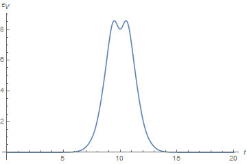
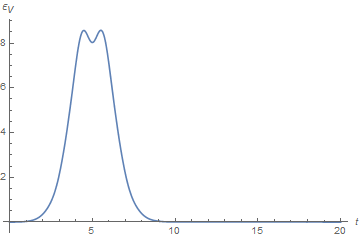
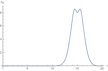
Figure 4: Left: Plot of $\epsilon_{V}$ as a function of time over one clock period $T_{0}$ with cosine potential $V_{0}(x)=A\cos^{2n}((x-x_{0})/2)$ from Section IX.2 with parameters $k_{0}=0$, $\sigma=\sqrt{d}$, $T_{0}=20$, $d=20$, $n=60$, $x_{0}=\pi$. The unitary is to be implemented at a time $t\approx x_{0}\,T_{0}/(2\pi)=T_{0}/2$ and the complex Gaussian superposition has its peak initially on the L.H.S. of the potential peak. Before the unitary is applied, to a time $t\approx 5$ the error is practically zero, during a period $t\approx 5$ to $t\approx 15$ the unitary is being applied and the error is large, but after $t\approx 15$, the unitary has been applied and the error is practically zero again. As one increases $n$ and $d$, the errors become arbitrarily small and the interval $t\in[5,15]$ in which there is a large error in the above plot becomes arbitrarily small. Middle and Right: Same as Left but changing $x_{0}$ to $\pi/2$ and $3\pi/2$ respectiverly, to illustrate how the same qualitative behaviour holds when the unitary is implemented at earlier and later times.

Intuition. The point of this Lemma is to make it manifest that the error invoked by using the finite dimensional Quasi-Ideal clock to control the quantum system on $\mathcal{H}_{s}$ (specifically, in this case, to perform an energy conserving unitary during a specific moment in time) is small. The two error terms on the r.h.s. of Eq. (297) involving $\varepsilon_{v}(t,d)$ decay fast with $d$ (see Eq. (257)) and only grow linearly in time. Note that $\epsilon_{V}(j\,T_{0},d)=0$ for all $d\in{\mathbbm{N}}^{+}$, $j\in{\mathbbm{N}}^{0}$. More generally, the error term $\epsilon_{V}$, will be small for a clock initially centered at $k_{0}$, at time $t$ when $V_{0}(2\pi(t/T_{0}+k_{0}/d))\approx V_{0}(2\pi t/T_{0})$, i.e. is relatively flat. Roughly speaking, this will be true for times $t$ before and after the unitary has been implemented as the example in Fig. 4 and the following lemma will make explicit. With a small modification, Lemma X.0.2 still holds if we do not assume the special choice of $g$ in Eq. (296). For general $g$, we simply replace $\epsilon_{k}$ in Eq. (298) with Eq. (317). The system dependency in Eq. (297) enters via the factor $\sqrt{d_{s}\mathrm{tr}[\rho_{s}^{2}(0)]}$ which varies between $\sqrt{d_{s}}$ for pure initial system states, and unity in the case of maximally mixed initial system states. The latter is what one should expect, since clearly an initially maximally mixed state is invariant under the unitary dynamics and as such the error associated with implementing a unitary should not depend on its dimension.

Proof.

Proceeding similarly to the derivation of Eq. (291) in the proof of Lemma X.0.1, we achieve

$$\rho_{s}(t)=\sum_{m,n=1}^{d_{s}}\rho_{m,n}(t)\braket{\bar{\Phi}_{n}(t)}{\bar{\Phi}_{m}(t)},$$ (299)

with

$$\ket{\bar{\Phi}_{l}(t)}:=\mathrm{e}^{-\mathrm{i}t(\hat{H}_{c}+\Omega_{l}\hat{V}_{d})}\ket{\Psi_{\textup{nor}}(k_{0})},\quad l=n,m.$$ (300)

Thus noting that the Frobenius norm, $\|\cdot\|_{F}$, is an upper bound to the trace distance $\|\cdot\|_{1}/\sqrt{d_{s}}$, for a $d_{s}$ dimensional system, followed by using Eq. (285),

$$\|\rho_{s}(t)-\rho_{s}^{\prime}(t)\|_{1} \leq\sqrt{d_{s}}\left|\left|\rho(t)-\rho^{\prime}(t)\right|\right|_{F}=\sqrt{d_{s}}\;\sqrt{\sum_{n,m}|\rho_{nm}(t)|^{2}\left|e^{-\mathrm{i}(\Omega_{m}-\Omega_{n})\int_{t_{i}}^{t_{f}}g(x)dx}-\braket{\bar{\Phi}_{n}(t)}{\bar{\Phi}_{m}(t)}\right|^{2}}$$ (301)

$$\leq\sqrt{d_{s}}\;\sqrt{\sum_{n,m}|\rho_{nm}(t)|^{2}\max_{q,r}\left\{\left|e^{-\mathrm{i}(\Omega_{q}-\Omega_{r})\int_{t_{i}}^{t_{f}}g(x)dx)}-\braket{\bar{\Phi}_{r}(t)}{\bar{\Phi}_{q}(t)}\right|^{2}\right\}}$$ (302)

$$\leq\sqrt{d_{s}\mathrm{tr}\left(\rho^{2}_{s}(0)\right)}\max_{q,r}\left\{\left|e^{-\mathrm{i}(\Omega_{q}-\Omega_{r})\int_{t_{i}}^{t_{f}}g(x)dx}-\braket{\bar{\Phi}_{r}(t)}{\bar{\Phi}_{q}(t)}\right|\right\}.$$ (303)

Applying Theorem IX.1,

$$\braket{\bar{\Phi}_{n}(t)}{\bar{\Phi}_{m}(t)}=\sum_{k\in\mathcal{S}(k_{0}+dt/T_{0})}\mathrm{e}^{-\mathrm{i}(\Omega_{n}-\Omega_{m})\int_{k-td/T_{0}}^{k}dyV_{d}(y)}\left|\psi_{\textup{nor}}(k_{0};k-td/T_{0})\right|^{2}+\tilde{\epsilon}_{n,m},$$ (304)

where

$$\tilde{\epsilon}_{n,m} =\braket{\bar{\Psi}_{\textup{nor}}(k_{0}+td/T_{0})}{\epsilon}+\braket{\epsilon}{\bar{\Psi}_{\textup{nor}}(k_{0}+td/T_{0})}+\braket{\epsilon}{\epsilon},$$ (305)

$$|\tilde{\epsilon}_{n,m}| \leq 2\varepsilon_{v}(t,d)+\varepsilon_{v}^{2}(t,d),\quad\forall n,m\,$$ (306)

with $\varepsilon_{v}(t,d)$ is given by Eq. (257). Note that the r.h.s of Eq. (305), does depend on indices $n$ and $m$. The r.h.s. of Eq. (306) on the other hand, is independent of $n$ and $m$.
Thus applying Eq. (306) to Eq. (303), we achieve

$$\frac{\|\rho_{s}(t)-\rho_{s}^{\prime}(t)\|_{1}}{\sqrt{d_{s}\mathrm{tr}[\rho^{2}_{s}(0)]}}\leq \max_{q,r}\left\{\left|1-\sum_{k\in\mathcal{S}(k_{0}+dt/T_{0})}\mathrm{e}^{\mathrm{i}(\Omega_{q}-\Omega_{r})\left(\int_{t_{i}}^{t_{f}}g(x)dx-\int_{k-td/T_{0}}^{k}dyV_{d}(y)\right)}\left|\psi_{\textup{nor}}(k_{0};k-td/T_{0})\right|^{2}\right|\right\}$$ (307)

$$+2\varepsilon_{v}(t,d)+\varepsilon_{v}^{2}(t,d)$$ (308)

$$\leq \max_{q\geq r}\left\{\left|1-\sum_{k\in\mathcal{S}(k_{0}+dt/T_{0})}\mathrm{e}^{\pm\mathrm{i}|\Omega_{q}-\Omega_{r}|\left(\int_{t_{i}}^{t_{f}}g(x)dx-\int_{k-td/T_{0}}^{k}dyV_{d}(y)\right)}\left|\psi_{\textup{nor}}(k_{0};k-td/T_{0})\right|^{2}\right|\right\}$$ (309)

$$+2\ \varepsilon_{v}(t,d)+\varepsilon_{v}^{2}(t,d)$$ (310)

$$= \max_{q,r}\left\{\rule{0.0pt}{28.45274pt}\right.\sqrt{\left(1-\sum_{k\in\mathcal{S}(k_{0}+dt/T_{0})}\cos(\pm g_{k}^{q,r})\left|\psi_{\textup{nor}}(k_{0};k-td/T_{0})\right|^{2}\right)^{2}+}$$ (311)

$$\,\,\quad\quad\,\,\,\,\,\,\,\,\overline{\left(\sum_{k\in\mathcal{S}(k_{0}+dt/T_{0})}\sin(\pm g_{k}^{q,r})\left|\psi_{\textup{nor}}(k_{0};k-td/T_{0})\right|^{2}\right)^{2}}\left.\rule{0.0pt}{28.45274pt}\right\}+2\varepsilon_{v}(t,d)+\varepsilon_{v}^{2}(t,d),$$ (312)

where

$$g_{k}^{q,r}:=|\Omega_{q}-\Omega_{r}|\left(\int_{t_{i}}^{t_{f}}g(x)dx-\int_{k-td/T_{0}}^{k}V_{d}(x)dx\right)\leq 2\pi\left|\int_{t_{i}}^{t_{f}}g(x)dx-\int_{k-td/T_{0}}^{k}V_{d}(x)dx\right|=:g_{k}\quad\forall\,q,r.$$ (313)

Thus using the identities $(|a|+|b|)^{2}\geq|a|^{2}+|b|^{2}$, $\sin(a)\leq|a|$, $-\cos(a)\leq a^{2}-1$, for $a,b\in{\mathbbm{R}}$, to achieve

$$\frac{\|\rho_{s}(t)-\rho_{s}^{\prime}(t)\|_{1}}{\sqrt{d_{s}\mathrm{tr}[\rho^{2}_{s}(0)]}}\leq \,2\varepsilon_{v}(t,d)+\varepsilon_{v}^{2}(t,d)+\sum_{k\in\mathcal{S}(k_{0}+dt/T_{0})}(g_{k}^{2}+g_{k})|\psi(k_{0};k-td/T_{0})|^{2}.$$ (314)

Performing the change of variable $y=k-td/T_{0}$, we find

$$\frac{\|\rho_{s}(t)-\rho_{s}^{\prime}(t)\|_{1}}{\sqrt{d_{s}\mathrm{tr}[\rho^{2}_{s}(0)]}}\leq \,2\varepsilon_{v}(t,d)+\varepsilon_{v}^{2}(t,d)+\sum_{y=\min\{\mathcal{S}(k_{0}+dt/T_{0})\}-td/T_{0}}^{\max\{\mathcal{S}(k_{0}+dt/T_{0})\}-td/T_{0}}(\epsilon_{y}^{2}+\epsilon_{y})|\psi(k_{0};y)|^{2}$$ (315)

$$\leq \,2\varepsilon_{v}(t,d)+\varepsilon_{v}^{2}(t,d)+\max_{\bar{\kappa}\in[0,1]}\sum_{y=k_{0}-d/2+\bar{\kappa}}^{k_{0}+d/2+\bar{\kappa}}(\epsilon_{y}^{2}+\epsilon_{y})|\psi(k_{0};y)|^{2},$$ (316)

where

$$\epsilon_{k}=2\pi\left|\int_{t_{i}}^{t}g(x)dx-\int_{k}^{k+td/T_{0}}V_{d}(x)dx\right|.$$ (317)

and to achieve the last line, we have used the inequalities

$$k_{0}-d/2+\bar{\kappa} \leq\min\{\mathcal{S}(k_{0}+dt/T_{0})\}-td/T_{0},$$ (318)

$$k_{0}+d/2+\bar{\kappa} \geq\max\{\mathcal{S}(k_{0}+dt/T_{0})\}-td/T_{0},$$ (319)

$$k_{0}+d/2+\bar{\kappa} -(k_{0}-d/2+\bar{\kappa})=d.$$ (320)

Finally, taking into account Eq. (296) followed by a change of variable, Eq. (317) can be written as

$$\epsilon_{k}=2\pi\left|\int_{0}^{t2\pi/T_{0}}V_{0}(x)dx-\int_{k}^{k+td/T_{0}}V_{d}(x)dx\right|=2\pi\left|\int_{0}^{t\,2\pi/T_{0}}dx\big{(}V_{0}(x)-V_{0}(x+2\pi k/d)\big{)}\right|.$$ (321)

∎

Corollary X.0.1 (Explicit form).

Let $V_{0}(x)\geq 0$ and have a unique global maximum in the interval $x\in[0,2\pi]$ at $x=x_{0}$ and $g$ be given by Eq. (296). Let $\tilde{\epsilon}_{V}$ be such that

$$1-\tilde{\epsilon}_{V}=\int_{x_{vl}}^{x_{vr}}dx\,V_{0}(x+x_{0})$$ (322)

for some $-\pi\leq x_{vl}<0<x_{vr}\leq\pi$, where, for simplicity, we assume $x_{vl}=-x_{vr}$. Let the initial Quasi-Ideal clock state be centered at zero; $k_{0}=0$, and introduce the parameter $0<\gamma_{\psi}\leq 1$. Furthermore, let $x_{0}$ be such that $x_{vr}+\pi\gamma_{\psi}\leq x_{0}\leq 2\pi-x_{vr}-\pi\gamma_{\psi}$. Then, for all times $t$ satisfying

$$\begin{split}0&\leq t\,2\pi/T_{0}\leq x_{0}-x_{vr}-\pi\gamma_{\psi}\end{split}$$ (323)

or

$$\begin{split}x_{0}+x_{vr}+\pi\gamma_{\psi}&\leq t\,2\pi/T_{0}\leq 2\pi+x_{0}-x_{vr}-\pi\gamma_{\psi},\end{split}$$ (324)

$\epsilon_{V}$ defined in Lemma X.0.2, is bounded by

$$\epsilon_{V}\leq 4\pi\left((1+2\pi)A^{2}\frac{\mathrm{e}^{-2\pi\tilde{\kappa}\frac{d^{2}}{\sigma^{2}}}}{1-\mathrm{e}^{-4\pi\sqrt{\tilde{\kappa}}\,d/\sigma^{2}}}+2\tilde{\epsilon}_{V}(1+8\pi\tilde{\epsilon}_{V})\right),\quad\tilde{\kappa}=\begin{cases}0&\mbox{if }d\gamma_{\psi}/2\leq 1\\ (\gamma_{\psi}/2-1/d)^{2}&\mbox{otherwise}\end{cases}$$ (325)

where $A$ is given by Eq. (25) and is a decreasing function of $\sigma$ (see Section E.1.1 for bounds).

Intuition. If the potential is very peaked around $x_{0}$ and close to zero away from $x_{0}$, then one can choose $x_{vl}\approx x_{vr}\approx 0$ with $0\leq\tilde{\epsilon}_{V}\ll 1$. Thus by choosing $\gamma_{\psi}\approx 0$, the intervals permitted for $x_{0}$ and $t$ by Eqs. (323) and Eqs. (324), are almost the full range $[0,2\pi]$ and $[0,T_{0}]$ respectively, and only for times $t\approx x_{0}T_{0}/(2\pi)$ will the error be large. Eqs. (323) correspond to the times before the unitary is applied, while Eqs. (324) correspond to the times after the unitary is applied.

Remark X.1.

The parameters $\gamma_{\psi},x_{vr}$ can be chosen to depend on $t$ and/or $d$ in order to improve bounds if desired.

Proof.

The proof consists in writing the sum in Eq. (298) in terms of three contributions; the left Gaussian tail of $|\psi_{\textup{nor}}(0;k)|$, the right Gaussian tail of $|\psi_{\textup{nor}}(0;k)|$, and the contribution from the center of the Gaussian $|\psi_{\textup{nor}}(0;k)|$. These terms are then all individually bounded.
Noting that $0\leq\epsilon_{k}\leq 2\pi$ and that $|\psi_{\textup{nor}}(0;k)|$ is normalized, we have from Eq. (298)

$$\epsilon_{V}(t,d)\leq\max_{\bar{\kappa}\in[0,1]}\Bigg{(} \sum_{k=-d/2+\bar{\kappa}}^{-d\gamma_{\psi}/2+\bar{\kappa}}\left(\epsilon_{k}^{2}+\epsilon_{k}\right)|\psi_{\textup{nor}}(k_{0};k)|^{2}+\sum_{k=d\gamma_{\psi}/2+\bar{\kappa}}^{d/2+\bar{\kappa}}\left(\epsilon_{k}^{2}+\epsilon_{k}\right)|\psi_{\textup{nor}}(k_{0};k)|^{2}$$ (326)

$$+\sum_{k=-d\gamma_{\psi}/2+1+\bar{\kappa}}^{d\gamma_{\psi}/2-1+\bar{\kappa}}\left(\epsilon_{k}^{2}+\epsilon_{k}\right)|\psi_{\textup{nor}}(k_{0};k)|^{2}\Bigg{)}$$ (327)

$$\leq 2\pi(1+2 \pi)\max_{\bar{\kappa}\in[0,1]}\bigg{(}\sum_{k=-d/2+\bar{\kappa}}^{-d\gamma_{\psi}/2+\bar{\kappa}}|\psi_{\textup{nor}}(k_{0};k)|^{2}+\sum_{k=d\gamma_{\psi}/2+\bar{\kappa}}^{d/2+\bar{\kappa}}|\psi_{\textup{nor}}(k_{0};k)|^{2}\bigg{)}$$ (328)

$$+\max_{\bar{\kappa}\in[0,1]} \max_{k\in\mathcal{I}_{\gamma_{\psi}}}\left(\epsilon_{k}^{2}+\epsilon_{k}\right),$$ (329)

where $\mathcal{I}_{\gamma_{\psi}}:=\{-d\gamma_{\psi}/2+1+\bar{\kappa},\,-d\gamma_{\psi}/2+2+\bar{\kappa},\ldots,d\gamma_{\psi}/2-1+\bar{\kappa}\}$.
First we will bound the terms in line 328. By a change of variable, followed by using Eq. (30), we find

$$2\pi(1+2\pi)\max_{\bar{\kappa}\in[0,1]}\bigg{(}\sum_{k=-d/2+\bar{\kappa}}^{-d\gamma_{\psi}/2+\bar{\kappa}}|\psi_{\textup{nor}}(k_{0};k)|^{2}+\sum_{k=d\gamma_{\psi}/2+\bar{\kappa}}^{d/2+\bar{\kappa}}|\psi_{\textup{nor}}(k_{0};k)|^{2}\bigg{)}$$ (330)

$$=2\pi(1+2\pi)A^{2}\max_{\bar{\kappa}\in[0,1]}\bigg{(}\sum_{x=0}^{d(1+\gamma_{\psi})/2}\mathrm{e}^{-\frac{2\pi}{\sigma^{2}}(x-d\gamma_{\psi}/2+\bar{\kappa})^{2}}+\sum_{x=0}^{d(1-\gamma_{\psi})/2}\mathrm{e}^{-\frac{2\pi}{\sigma^{2}}(x+d\gamma_{\psi}/2+\bar{\kappa})^{2}}\bigg{)}$$ (331)

$$\leq 2\pi(1+2\pi)A^{2}\max_{\bar{\kappa}\in[0,1]}\bigg{(}\frac{\mathrm{e}^{-\frac{2\pi}{\sigma^{2}}(d\gamma_{\psi}/2-\bar{\kappa})^{2}}}{1-\mathrm{e}^{-4\pi|d\gamma_{\psi}/2-\bar{\kappa}|/\sigma^{2}}}+\frac{\mathrm{e}^{-\frac{2\pi}{\sigma^{2}}(d\gamma_{\psi}/2+\bar{\kappa})^{2}}}{1-\mathrm{e}^{-4\pi|d\gamma_{\psi}/2+\bar{\kappa}|/\sigma^{2}}}\bigg{)}$$ (332)

$$\leq 4\pi(1+2\pi)A^{2}\frac{\mathrm{e}^{-2\pi\tilde{\kappa}\frac{d^{2}}{\sigma^{2}}}}{1-\mathrm{e}^{-4\pi\sqrt{\tilde{\kappa}}\,d/\sigma^{2}}},$$ (333)

with $\tilde{\kappa}:=\min_{\bar{\kappa}\in[0,1]}\{(\gamma_{\psi}/2-\bar{\kappa}/d)^{2},(\gamma_{\psi}/2+\bar{\kappa}/d)^{2}\}=\min_{\bar{\kappa}\in[0,1]}(\gamma_{\psi}/2-\bar{\kappa}/d)^{2}$ and where in line 332, the bound from Lemma E.0.1 has been used.
Now we will bound the term in line 329. By the change of variables $y=x-x_{0}$, $y^{\prime}=x+2\pi k/d-x_{0}$, Eq. (298) can be written in the form

$$\epsilon_{k}=2\pi\left|\int_{-x_{0}}^{t\,2\pi/T_{0}-x_{0}}dx\,V_{0}(x-x_{0})-\int_{\frac{2\pi}{d}k-x_{0}}^{t\,2\pi/T_{0}+\frac{2\pi}{d}k-x_{0}}dx\,V_{0}(x-x_{0})\right|.$$ (334)

Taking into account that

$$1=\int_{-\pi}^{\pi}dxV_{0}(x+x_{0}),$$ (335)

together with Eq. (322) and the periodicity of the potential, it follows that

$$\tilde{\epsilon}_{V}=\int_{x_{vr}-2\pi}^{x_{vl}}dxV_{0}(x+x_{0}).$$ (336)

Thus from Eq. (334), we have that $\epsilon_{k}\leq 4\pi\tilde{\epsilon}_{V}$ if

$$\begin{split}x_{vr}-2\pi\leq-x_{0}&\leq t2\pi/T_{0}-x_{0}\leq x_{vl}\\ x_{vr}-2\pi\leq-x_{0}\leq 2\pi\frac{k}{d}-x_{0}&\leq t2\pi/T_{0}+2\pi\frac{k}{d}-x_{0}\leq x_{vl}\quad\forall\,k\in\mathcal{I}_{\gamma_{\psi}}.\end{split}$$ (337)

Taking into account $t\geq 0$ and that $\min\mathcal{I}_{\gamma_{\psi}}=\bar{\kappa}-d\gamma_{\psi}/2+1$, $\max\mathcal{I}_{\gamma_{\psi}}=\bar{\kappa}+d\gamma_{\psi}/2-1$, Eqs. (337) are implied by Eqs. (323). To derive Eqs. (324), we first note that

$$\epsilon_{k}= 2\pi\Bigg{|}\int_{-x_{0}}^{x_{vl}}dx\,V_{0}(x+x_{0})+\int_{x_{vl}}^{x_{vr}}dx\,V_{0}(x+x_{0})+\int_{x_{vr}}^{t\,2\pi/T_{0}-x_{0}}dx\,V_{0}(x+x_{0})$$ (338)

$$-\int_{\frac{2\pi}{d}k-x_{0}}^{x_{vl}}dx\,V_{0}(x+x_{0})-\int_{x_{vl}}^{x_{vr}}dx\,V_{0}(x+x_{0})-\int_{x_{vr}}^{t\,2\pi/T_{0}+\frac{2\pi}{d}k-x_{0}}dx\,V_{0}(x+x_{0})\Bigg{|}$$ (339)

$$\leq 2\pi\Bigg{|}\int_{-x_{0}}^{x_{vl}}dx\,V_{0}(x+x_{0})\Bigg{|}+2\pi\Bigg{|}\int_{x_{vr}}^{t\,2\pi/T_{0}-x_{0}}dx\,V_{0}(x+x_{0})\Bigg{|}$$ (340)

$$+2\pi\Bigg{|}\int_{\frac{2\pi}{d}k-x_{0}}^{x_{vl}}dx\,V_{0}(x+x_{0})\Bigg{|}+2\pi\Bigg{|}\int_{x_{vr}}^{t\,2\pi/T_{0}+\frac{2\pi}{d}k-x_{0}}dx\,V_{0}(x+x_{0})\Bigg{|}.$$ (341)

In order for $\epsilon_{k}$, $k\in\mathcal{I}_{\gamma_{\psi}}$ to be bounded by $8\pi\tilde{\epsilon}_{V}$, the following conditions derived from Eq. (338) are sufficient:

$$\begin{split}x_{vr}-2\pi&\leq-x_{0}\leq x_{vl}\\ x_{vr}-2\pi&\leq\frac{2\pi}{d}k-x_{0}\leq x_{vl}\quad\forall\,k\in\mathcal{I}_{\gamma_{\psi}}\end{split}$$ (342)

and

$$\begin{split}x_{vr}&\leq t2\pi/T_{0}-x_{0}\leq x_{vl}+2\pi\\ x_{vr}&\leq t2\pi/T_{0}+\frac{2\pi}{d}k-x_{0}\leq x_{vl}+2\pi\quad\forall\,k\in\mathcal{I}_{\gamma_{\psi}}.\end{split}$$ (343)

Eqs. (342), (343) are implied by Eq. (324). Thus whenever Eqs. (323) or Eqs. (324) are satisfied, the last term in Eq. (326) is bounded by

$$\max_{\bar{\kappa}\in[0,1]}\max_{k\in\mathcal{I}_{\gamma_{\psi}}}\left(\epsilon_{k}^{2}+\epsilon_{k}\right)\leq 8\pi\tilde{\epsilon}_{V}(8\pi\tilde{\epsilon}_{V}+1),$$ (344)

∎

Finally, via the following corollary, we will now show how up to a small correction, the bounds derived in Lemma X.0.2 are the same for $g$ as defined in Section IV.4. The asymptotic bounds in the large $d$ limit for the fidelity of the unitary implementation of the system reported in Section IV.4, will then be derived in the next Section, X.3.1.

Corollary X.0.2 (Section IV.4 form).

Let $V_{0}$ and $\tilde{\epsilon}_{V}$ satisfy the same conditions as in Corollary X.0.1, and let $g$ be the normalised pulse from Section X.1 with support interval $[t_{i},t_{f}]=[t_{1},t_{2}]$ , then for all $t\in[0,t_{1}]\cup[t_{2},T_{0}]$ and $0<t_{1}<t_{2}<T_{0}$,

$$\|\rho_{s}(t)-\rho^{\prime}_{s}(t)\|_{1}\leq\sqrt{d_{s}\mathrm{tr}[\rho_{s}^{2}(0)]}\left(2\varepsilon_{v}(t,d)+\varepsilon_{v}^{2}(t,d)+\varepsilon_{s}(t,d)\right),$$ (345)

where

$$\varepsilon_{s}(t,d):= \epsilon_{V}(d)+2\pi T_{0}\tilde{\epsilon}_{V}(2\pi T_{0}\tilde{\epsilon}_{V}+1),$$ (346)

$$x_{0}= \frac{t_{2}+t_{1}}{2}\frac{2\pi}{T_{0}},$$ (347)

and $0<\gamma_{\psi}\leq 1\,$, $0<x_{vr}\leq\pi$ are any combination satisfying

$$x_{vr}+\pi\gamma_{\psi}=\frac{t_{2}-t_{1}}{2}\frac{2\pi}{T_{0}}.$$ (348)

Furthermore, $\epsilon_{V}(d)$ is bounded by Eq. (325), and $\tilde{\epsilon}_{V}$ satisfies Eq. (322). $\rho_{s}(t)$ is given by Eq. (281) and $\rho^{\prime}_{s}(t)=\mathrm{tr}_{c}[\rho^{\prime}_{sc}(t)]$ by Eq. (295).

Proof.

Let $g_{1}$ denoted $g$ as defined in this Corollary and $g_{2}$ denote $g$ as defined via Eq. (296). With these functions, define $\epsilon_{g}(t)=\int_{0}^{t}dx(g_{2}(x)-g_{1}(x))$, $\rho_{S,q}(t)=U_{q}(t)\rho_{s}(0)U_{q}^{\dagger}(t),$ $U_{q}(t)=\mathrm{e}^{-\mathrm{i}\hat{H}_{s}^{int}\int_{0}^{t}g_{q}(t)}$, $q=1,2$. First note

$$\int_{t_{1}}^{t_{2}}dxg_{2}(x)=\frac{2\pi}{T_{0}}\int_{t_{1}}^{t_{2}}dxV_{0}(x2\pi/T_{0})=\int_{-x_{vr}-\pi\gamma_{\psi}}^{x_{vr}+\pi\gamma_{\psi}}dxV_{0}(x+x_{0})\geq\int_{-x_{vr}}^{x_{vr}}dxV_{0}(x+x_{0})=1-\tilde{\epsilon}_{V}.$$ (349)

Thus

$$1=\int_{0}^{T_{0}}dx\,g_{2}(x)\geq\int_{0}^{t_{1}}dx\,g_{2}(x)+1-\tilde{\epsilon}_{V}+\int_{t_{2}}^{T_{0}}dx\,g_{2}(x)\implies\tilde{\epsilon}_{V}\geq\begin{cases}\int_{0}^{t_{1}}dx\,g_{2}(x)\\ \vspace{-0.3cm}\\ \int_{t_{2}}^{T_{0}}dx\,g_{2}(x)\end{cases}$$ (350)

Using Eq. (350), $\|\cdot\|_{1}/\sqrt{d_{s}}\leq\|\cdot\|_{F}$, where $\|\cdot\|_{F}$ is the Frobenius norm for a $d_{s}$ dimensional system, and the bounds $\sin(a)\leq|a|$, $-\cos(a)\leq a^{2}-1$, $a\in{\mathbbm{R}}$, we find

$$\|\rho_{s,1}(t)-\rho_{s,2}(t)\|_{1} =\|\rho_{s}(0)-U_{1}^{\dagger}U_{2}(t)\rho_{s}(0)U_{2}^{\dagger}U_{1}(t)\|_{1}\leq\sqrt{d_{s}}\|\rho_{s}(0)-U_{1}^{\dagger}U_{2}(t)\rho_{s}(0)U_{2}^{\dagger}U_{1}(t)\|_{F}$$ (351)

$$=\sqrt{d_{s}}\sqrt{\sum_{m,n}\big{|}\rho_{m,n}(t)-\mathrm{e}^{-\mathrm{i}(\Omega_{m}-\Omega_{n})\epsilon_{g}(t)}\rho_{m,n}(t)\big{|}^{2}}\leq\sqrt{d_{s}\mathrm{tr}[\rho_{s}^{2}(0)]}\max_{m,n}|1-\mathrm{e}^{-\mathrm{i}(\Omega_{m}-\Omega_{n})\epsilon_{g}(t)}|$$ (352)

$$\leq 2\pi(2\pi|\epsilon_{g}(t)|+1)|\epsilon_{g}(t)|.$$ (353)

Using Eq. (350), we thus conclude $|\epsilon_{g}(t)|\leq\tilde{\epsilon}_{V}T_{0}$, for $t\in[0,t_{1}]\cup[t_{2},T_{0}]$. Finally, note that $\|\rho_{s}(t)-\rho_{s,1}(t)\|_{1}\leq\|\rho_{s}(t)-\rho_{s,2}(t)\|_{1}+\|\rho_{s,1}(t)-\rho_{s,2}(t)\|_{1}$ via the triangle inequality. $\|\rho_{s}(t)-\rho_{s,2}(t)\|_{1}$ was bounded in Eq. (297), with $\epsilon_{V}(t,d)$ bounded in Corollary X.0.1 for $t\in[0,t_{1}]\cup[t_{2},T_{0}]$. Using these two bounds and Eq. (351), Eq, (345) follows. To finalize the proof, note that $x_{0}=\frac{t_{2}+t_{1}}{2}\frac{2\pi}{T_{0}}$, $x_{vr}+\pi\gamma_{\psi}=\frac{t_{2}-t_{1}}{2}\frac{2\pi}{T_{0}}$. As such, the condition $x_{vr}+\pi\gamma_{\psi}\leq x_{0}\leq 2\pi-x_{vr}-\pi\gamma_{\psi}$ from Lemma X.0.1 is satisfied for all $0<t_{1}<t_{2}<T_{0}$ and Eq. (325) is valid. ∎

X.3.1 Examples

We can now bound $\tilde{\epsilon}_{V}$ for the cosine potential defined in Section IX.2 with the aim of understanding the significance of Corollaries X.0.1, X.0.2. We find the bound

$$\tilde{\epsilon}_{V}\leq\frac{(\pi-x_{vr})\mathrm{e}^{2}}{4\pi\sqrt{\pi}}\sqrt{n}\cos^{2n}(x_{vr}/2),\quad\text{if }\cos(x_{vr})\leq 1-\frac{1}{n}.$$ (354)

A proof of Eq. (354) can be found in appendix D. By choosing $n=n(d)$ in different ways, one can achieve different decay rates. This choice will also effect the decay rates of $\varepsilon_{v}(t,d)$ defined in Eq. 257, the significance of which will be clarified in Section X.5. We give three examples of $n=n(d)$:

• Power law decay. Let

  $$n=\gamma_{1}\frac{\ln d}{-2\ln\cos(x_{vr}/2)},\quad\gamma_{1}>0.$$ (355)

  Then

  $$\tilde{\epsilon}_{V}\leq\frac{(\pi-x_{vr})\mathrm{e}^{2}}{4\pi\sqrt{\pi}}\sqrt{\gamma_{1}\frac{\ln d}{-2\ln\cos(x_{vr}/2)}}\,d^{-\gamma_{1}},$$ (356)

  if

  $$\gamma_{1}\geq\frac{-2\ln\cos(x_{vr}/2)}{\left(1-\cos(x_{vr})\right)}\frac{1}{\ln d}.$$ (357)

  Note that $\lim_{d\rightarrow\infty}\tilde{\epsilon}_{V}d^{m}=0$ for all $\gamma_{1}>m>0$. Using the definition of the clock rate parameter $\bar{\upsilon}$ (Def. 9), we find

  $$\bar{\upsilon}=\frac{\ln d}{\ln(\pi\alpha_{0}\sigma^{2})}\frac{2\mathrm{e}^{2}}{(2\pi)^{3/2}\sqrt{2}}\frac{\pi\kappa\alpha_{0}}{(-2\ln\cos(x_{vr}/2))^{3/2}}\gamma_{1}^{3/2}\sqrt{\ln d}.$$ (358)

  Thus from Eq. (257), for $\sigma=\sqrt{d}$,

  $$\varepsilon_{v}(t,d)=\mathcal{O}\left(t\,poly(d)\,\exp\left(-\frac{\pi}{4}\frac{\alpha_{0}^{2}\chi_{1}^{2}\gamma_{1}^{3}}{\left(1+\chi_{1}\gamma_{1}^{3/2}/\sqrt{\ln d}\right)^{2}}\frac{d}{\ln d}\right)\right),\quad\text{as }\,\,d\rightarrow\infty$$ (359)

  with

  $$\chi_{1}:=\frac{(2\pi)^{3/2}\sqrt{2}}{2\,\mathrm{e}^{2}}\left(1+\frac{\ln(\pi\alpha_{0})}{\ln d}\right)\frac{\left(-2\ln(\cos x_{vr}/2)\right)^{3/2}}{\pi\kappa\alpha_{0}}.$$ (360)

  Furthermore, using Eq. (325), for Eqs. (297), (345) one has that

  $$\frac{\|\rho_{s}(t)-\rho^{\prime}_{s}(t)\|_{1}}{\sqrt{d_{s}\mathrm{tr}[\rho_{s}^{2}(0)]}}=\mathcal{O}\left(\varepsilon_{v}(t,d)\right)+\mathcal{O}\left(\mathrm{e}^{-2\pi\tilde{k}(d/\sigma)^{2}}\right)+\mathcal{O}\left(\tilde{\epsilon}_{V}\right),\quad\text{as }\,\,d\rightarrow\infty.$$ (361)

  Thus since $\varepsilon_{v}(t,d)$ decays faster than any power of $d$, for $\sigma=\sqrt{d}$ and any $\gamma_{\psi}\in(0,1]$, we have that

  $$\lim_{d\rightarrow\infty}\|\rho_{s}(t)-\rho^{\prime}_{s}(t)\|_{1}\,d^{m}=0,$$ (362)

  for all constants $\gamma_{1}>m>0$.

• System error faster than power-law decay. By parametrizing $\gamma_{1}$ in example 1) to increase sufficiently slowly with $d$ rather than being constant, we can achieve that the trace distance error between $\rho_{s}$ and $\rho_{s}^{\prime}$ (Eqs. (297) and (345)) decays with $d$ faster than any power law in $d^{m}$ for the optimal clock decay $\sigma=\sqrt{d}$. The penalty of this improvement, will be a worse decay rate for $\varepsilon_{v}(t,d)$ than that of Eq. (359) . Let

  $$\gamma_{1}=\frac{\pi}{4}\alpha_{0}^{2}\chi_{2}^{2}\frac{d^{1/4}}{\sqrt{\ln d}},\quad\chi_{2}:=\chi_{1}\left(\frac{\pi}{4}\alpha_{0}^{2}\chi_{1}^{2}\right)^{-3/8}.$$ (363)

  such that Eq. (357) is satisfied, then for $\sigma=\sqrt{d}$,

  $$\varepsilon_{v}(t,d) =\mathcal{O}\left(t\,poly(d)\,\,\mathrm{e}^{-\frac{\pi}{4}\alpha_{0}^{2}\chi_{2}^{2}\,d^{1/4}\sqrt{\ln d}}\,\right),\quad\text{as }\,\,d\rightarrow\infty,$$ (364)

  $$\tilde{\epsilon}_{V} \leq\frac{(\pi-x_{vr})\mathrm{e}^{2}\alpha_{0}\chi_{2}}{8\pi}\frac{(d\ln d)^{1/4}}{\sqrt{-2\ln\cos(x_{vr}/2)}}\,\mathrm{e}^{-\frac{\pi}{4}\alpha_{0}^{2}\chi_{2}^{2}\,d^{1/4}\sqrt{\ln d}},$$ (365)

  and thus up to polynomial factors, both $\varepsilon_{v}(t,d)$ and $\tilde{\epsilon}_{V}$ have exponential decay in $d^{1/4}\sqrt{\ln d}$ and

  $$\frac{\|\rho_{s}(t)-\rho^{\prime}_{s}(t)\|_{1}}{\sqrt{d_{s}\mathrm{tr}[\rho_{s}^{2}(0)]}}=\mathcal{O}\left(\left(t\,poly(d)+(d\ln d)^{1/4}\right)\mathrm{e}^{-\frac{\pi}{4}\alpha_{0}^{2}\chi_{2}^{2}\,d^{1/4}\sqrt{\ln d}}\,\right),$$ (366)

  from which we conclude

  $$\lim_{d\rightarrow\infty}\|\rho_{s}(t)-\rho_{s}^{\prime}(t)\|_{1}\,d^{m}=\lim_{d\rightarrow\infty}\varepsilon_{v}(t,d)\,d^{m}=0,$$ (367)

  for all constant $m>0$ and for all $t$ such that Eq. (323) and Eq. (324) hold. Furthermore, the constraint of Eq. (357) can be re-written in terms of the new parametrizations to achieve, using Eqs. (357) and (363) the constraint

  $$\frac{4}{\pi\alpha_{0}^{2}\chi_{2}^{2}}\frac{-2\ln\cos(x_{vr}/2)}{1-\cos(x_{vr})}\leq d^{1/4}\sqrt{\ln d}.$$ (368)

  This constraint is satisfied for all constant $x_{vr}\in(0,2\pi)$ for sufficiently large $d$ (recall that by definition, $\chi_{2}$ depends on $x_{vr}$). Similarly, $\gamma_{\psi}$ can be any constant in $(0,1)$.

• Smallest clock error. In this case, we will bound how quickly the error $\tilde{\epsilon}_{V}$ can decay with $d$ while maintaining the smallest disturbance imposed on the clock due to performing the unitary (see section X.5 for details), that is to say, while maintaining a constant rate parameter $\bar{\upsilon}$, for the optimal clock decay $\sigma=\sqrt{d}$.
  Let

  $$n=\frac{\gamma_{3}}{-2\ln\cos(x_{vr})}(\ln d)^{2/3},\quad\gamma_{3}>0.$$ (369)

  Then $\tilde{\epsilon}_{V}$ decays with increasing $d$ at a rate

  $$\tilde{\epsilon}_{V}\leq\frac{(\pi-x_{vr})\mathrm{e}^{2}}{4\pi\sqrt{\pi}}\sqrt{\frac{\gamma_{3}}{-2\ln\cos(x_{vr})}}(\ln d)^{2/3}d^{-\gamma_{3}(\ln d)^{-1/3}},\quad\text{if }\gamma_{3}\geq\frac{-2\ln\cos(x_{vr})}{\left(1-\cos(x_{vr})\right)}\frac{1}{(\ln d)^{2/3}},$$ (370)

  and the clock rate parameter (Def. 9) is

  $$\bar{\upsilon}=\frac{\ln d}{\ln(\pi\alpha_{0}\sigma^{2})}\frac{2\mathrm{e}^{2}}{(2\pi)^{3/2}\sqrt{2}}\frac{\pi\kappa\alpha_{0}}{(-2\ln\cos(x_{vr}))^{3/2}}\gamma_{3}^{3/2},$$ (371)

  which is bounded in the $d\rightarrow\infty$ limit. Thus for this parametrisation, $\varepsilon_{v}(t,d)$ has exponential decay in $d$ and consequently the clock’s disturbance decays exponentially when $\sigma=\sqrt{d}$, (recall Theorem IX.1).

X.4 How to perform any timed unitary

So far we have concerned ourselves with performing energy preserving unitaries only. Often, one may want to perform any unitary on the system $\mathcal{H}_{s}$. The clock provides a source of timing, but not energy. To perform non-energy preserving unitaries, one will need an energy source. To achieve this, one can introduce a battery system with Hilbert space $\mathcal{H}_{b}$. Then, the clock can perform energy preserving unitaries on a state $\rho_{sb}$ on $\mathcal{H}_{s}\otimes\mathcal{H}_{b}$ according the procedure described in Section X.3. The initial state of the battery is chosen such that it has enough energy to implement the unitary and will be such that an energy preserving unitary over $U_{sb}$ on a state $\rho_{s}\otimes\rho_{b}$ will induce any desired unitary $U^{\prime}_{s}$, on $\rho_{s}$, namely $\mathrm{tr}_{b}[U_{sb}\rho_{s}\otimes\rho_{b}U_{sb}^{\dagger}]=U^{\prime}_{s}\rho_{s}U^{\prime{\dagger}}_{s}$, where $[U_{sb},\hat{H}_{s}\otimes{\mathbbm{1}}_{b}+{\mathbbm{1}}_{s}\otimes\hat{H}_{s}]=0$, $[U^{\prime}_{s},\hat{H}_{s}]\neq 0$. The procedure which allows one to find a state $\rho_{b}\in\mathcal{S}(\mathcal{H}_{b})$, a Hamiltonian $\hat{H}_{b}$ on $\mathcal{H}_{b}$ and an energy preserving unitary $U_{sb}$ on $\mathcal{H}_{sb}$, such that any desired unitary $U^{\prime}_{s}$ on $\mathcal{H}_{s}$ can be performed, is the topic of Aberg . Therefore, using the finite dimension clock together with a battery as discussed in this Section, one can achieve any timed non-energy preserving unitary on states on $\mathcal{H}_{s}$ using the results of Aberg . This will be developed with explicit error bounds in an upcoming paper.

X.5 Clock Fidelity

If the potential $V_{0}(x)$ is zero for all $x\in{\mathbbm{R}}$, then the system on $\mathcal{H}_{s}$ and the clock on $\mathcal{H}_{c}$ will evolve in time as non-interacting systems. After a time $T_{0}$, as we have seen, the clock state will return to its initial state. However, whenever $V_{0}(x)\neq 0$ for some $x\in{\mathbbm{R}}$, the system-clock interaction will disturb the dynamics of the clock such that after a time $T_{0}$, the clock state will not have returned to its initial state. Lemma X.0.3 in this Section bounds quantitatively how large this disturbance is, and how quickly it decays with clock dimension.

Lemma X.0.3 (Clock disturbance).

Let $\rho_{c}^{\prime}(t):=\mathrm{tr}_{s}[\rho_{sc}^{\prime}(t)]$, ($\rho_{sc}^{\prime}$ defined in Eq. (295)), be the state of the clock at time $t$. We have the bound,

$$\frac{1}{2}\|\rho_{c}^{\prime}(0)-\rho_{c}^{\prime}(T_{0})\|_{1}\leq\varepsilon_{v}(T_{0},d),$$ (372)

where $\varepsilon_{v}(\cdot,\cdot)$ is defined in Eq. (257).

Intuition The bound on the trace distance given by Eq. (372), decays quickly with $d$ while increasing linearly in $T_{0}$ as is evident from the definition of $\varepsilon_{v}(\cdot,\cdot)$. It bounds the disturbance which is only originating from the implementation of the unitary on the system on $\mathcal{H}_{s}$, since $\|\rho_{c}^{\prime}(0)-\rho_{c}^{\prime}(T_{0})\|_{1}=0$ if $V_{0}(x)=0$ for all $x\in{\mathbbm{R}}$.

Proof.

The result follows from Theorem 255 and simple identities.
By taking the partial trace over the system Hilbert space $\mathcal{H}_{s}$, from Eq. (295) we achieve

$$\rho_{sc}^{\prime}(t)=\sum_{m,n=1}^{d_{s}}\rho_{m,n}(t)\ket{\phi_{m}}\!\!\bra{\phi_{n}}\otimes\ket{\bar{\Phi}_{m}(t)}\!\!\bra{\bar{\Phi}_{n}(t)}_{c},$$ (373)

where we have used definitions Eqs. (284), (300). Taking the partial trace over the system Hilbert space $\mathcal{H}_{s}$, we achieve

$$\rho_{c}^{\prime}(t)=\sum_{n=1}^{d_{s}}\rho_{n,n}(0)\ket{\bar{\Phi}_{n}(t)}\!\!\bra{\bar{\Phi}_{n}(t)}_{c}.$$ (374)

Thus the quantum Fidelity $F$ is

$$F(\rho_{c}^{\prime}(0),\rho_{c}^{\prime}(t)) =\mathrm{tr}\left[\sqrt{\sqrt{\rho_{c}^{\prime}(0)}\rho_{c}^{\prime}(t)\sqrt{\rho_{c}^{\prime}(t)}}\right]$$ (375)

$$=\mathrm{tr}\left[\sqrt{\ket{\Psi_{\textup{nor}}(k_{0})}\!\!\bra{\Psi_{\textup{nor}}(k_{0})}\left(\sum_{n=1}^{d_{s}}\rho_{n,n}(0)\hat{\Gamma}_{n}(t)\ket{\Psi_{\textup{nor}}(k_{0})}\!\!\bra{\Psi_{\textup{nor}}(k_{0})}\hat{\Gamma}_{n}^{\dagger}(t)\right)\ket{\Psi_{\textup{nor}}(k_{0})}\!\!\bra{\Psi_{\textup{nor}}(k_{0})}}\right]$$ (376)

$$=\mathrm{tr}\left[\sqrt{\ket{\Psi_{\textup{nor}}(k_{0})}\!\!\bra{\Psi_{\textup{nor}}(k_{0})}\left(\sum_{n=1}^{d_{s}}\rho_{n,n}(0)\left|\bra{\Psi_{\textup{nor}}(k_{0})}\hat{\Gamma}_{n}(t)\ket{\Psi_{\textup{nor}}(k_{0})}\right|^{2}\right)}\right]$$ (377)

$$=\sqrt{\sum_{n=1}^{d_{s}}\rho_{n,n}(0)\left|\bra{\Psi_{\textup{nor}}(k_{0})}\hat{\Gamma}_{n}(t)\ket{\Psi_{\textup{nor}}(k_{0})}\right|^{2}},$$ (378)

where we have defined

$$\hat{\Gamma}_{n}(t):=\mathrm{e}^{-\mathrm{i}t(\hat{H}_{c}+\Omega_{n}\hat{V}_{d})}.$$ (379)

Applying Theorem 255, we find

$$\left|\bra{\Psi_{\textup{nor}}(k_{0})}\hat{\Gamma}_{n}(T_{0})\ket{\Psi_{\textup{nor}}(k_{0})}\right|^{2} =\left(\mathrm{e}^{-\mathrm{i}\Omega_{n}}+\braket{\Psi_{\textup{nor}}(k_{0})}{\epsilon_{n}}\right)\left(\mathrm{e}^{-\mathrm{i}\Omega_{n}}+\braket{\Psi_{\textup{nor}}(k_{0})}{\epsilon_{n}}\right)^{*}$$ (380)

$$=1+\braket{\Psi_{\textup{nor}}(k_{0})}{\epsilon_{n}}\mathrm{e}^{+\mathrm{i}\Omega_{n}}+\braket{\epsilon_{n}}{\Psi_{\textup{nor}}(k_{0})}\mathrm{e}^{-\mathrm{i}\Omega_{n}}+|\braket{\epsilon_{n}}{\Psi_{\textup{nor}}(k_{0})}|^{2}$$ (381)

$$\geq 1+\braket{\Psi_{\textup{nor}}(k_{0})}{\epsilon_{n}}\mathrm{e}^{+\mathrm{i}\Omega_{n}}+\braket{\epsilon_{n}}{\Psi_{\textup{nor}}(k_{0})}\mathrm{e}^{-\mathrm{i}\Omega_{n}}.$$ (382)

However,

$$1=\left|\bra{\Psi_{\textup{nor}}(k_{0})}\Gamma_{n}^{\dagger}(T_{0})\Gamma_{n}(T_{0})\ket{\Psi_{\textup{nor}}(k_{0})}\right|^{2}=\left(\bra{\Psi_{\textup{nor}}(k_{0})}\mathrm{e}^{\mathrm{i}\Omega_{n}}+\bra{\epsilon_{n}}\right)\left(\mathrm{e}^{-\mathrm{i}\Omega_{n}}\ket{\Psi_{\textup{nor}}(k_{0})}+\ket{\epsilon_{n}}\right)$$ (383)

$$\implies \braket{\Psi_{\textup{nor}}(k_{0})}{\epsilon_{n}}\mathrm{e}^{+\mathrm{i}\Omega_{n}}+\braket{\epsilon_{n}}{\Psi_{\textup{nor}}(k_{0})}\mathrm{e}^{-\mathrm{i}\Omega_{n}}=-\braket{\epsilon_{n}}{\epsilon_{n}}=-||\ket{\epsilon_{n}}||^{2}_{2},$$ (384)

Thus from Eq. (380), we achieve

$$\left|\bra{\Psi_{\textup{nor}}(k_{0})}\hat{\Gamma}_{n}(T_{0})\ket{\Psi_{\textup{nor}}(k_{0})}\right|^{2}\geq 1-||\ket{\epsilon_{n}}||^{2}_{2}.$$ (385)

Plunging into Eq. (375),

$$F(\rho_{c}^{\prime}(0),\rho_{c}^{\prime}(T_{0}))\geq\sqrt{\sum_{n=1}^{d_{s}}\rho_{n,n}(0)\left(1-||\ket{\epsilon_{n}}||^{2}_{2}\right)}\geq\sqrt{\min_{n\in{1,\ldots,d_{s}}}\left(1-||\ket{\epsilon_{n}}||^{2}_{2}\right)}=\sqrt{1-\varepsilon_{v}^{2}(T_{0},d)},$$ (386)

where $\varepsilon_{v}(\cdot,\cdot)$ is defined in Eq. (257). Thus we conclude the Lemma using the well known relationship between Fidelity and trace distance, namey $\frac{1}{2}\|\rho-\sigma\|_{1}\leq\sqrt{1-F^{2}(\rho,\sigma)}$, for two quantum states $\rho$, $\sigma$.∎

XI Commutator relations for the Quasi-Ideal clock states

For simplicity, in this section we will assume the dimension $d$ to be odd, and shift spectrum of $\hat{H}_{c}$ and $\hat{t}_{c}$ to be centered at zero, giving us

$$\hat{H}_{c} =\sum_{n=-\frac{d-1}{2}}^{+\frac{d-1}{2}}n\frac{2\pi}{T_{0}}\ket{E_{n}}\!\!\bra{E_{n}}, \hat{t}_{c} =\sum_{k=-\frac{d-1}{2}}^{+\frac{d-1}{2}}k\frac{T_{0}}{d}\ket{\theta_{k}}\!\!\bra{\theta_{k}}.$$ (387)

The shifting of the spectrum clearly has no physical effect on the dynamics nor the commutator of these operators since the ground state and initial time can be sifted back to zero by simply adding a term proportional to the identity operator to the r.h.s. of $\hat{H}_{c}$ and $\hat{t}_{c}$. The mean energy of the state $n_{0}$ before defined on $n_{0}\in(0,d-1)$ in this section is now shifted to $n_{0}\in\left(-\frac{d}{2},\frac{d}{2}\right)$. We will also assume $k_{0}\in\left(-\frac{d}{2},\frac{d}{2}\right)$ in this section for simplicity and define.

$$\bar{\alpha} =\left|\frac{2n_{0}}{d}\right|, \bar{\beta} =\left|\frac{2k_{0}}{d}\right|.$$ (388)

Thus both $\bar{\alpha},\bar{\beta}\in[0,1)$. They are both measures of how close to the edge of the spectra of $\hat{H}_{c}$ and $\hat{t}_{c}$ the state is; c.f. similar measure Def. (2).

Theorem XI.1 (Quasi-Canonical commutation).

For all states $\ket{\Psi_{\textup{nor}}(k_{0})}\in\Lambda_{\sigma,n_{0}}$, the time operator $\hat{t}_{c}$ and Hamiltonian $\hat{H_{c}}$ satisfy the commutation relation

$$\left[\hat{t}_{c},\hat{H}_{c}\right]\ket{\Psi_{\textup{nor}}(k_{0})} =\mathrm{i}\ket{\Psi_{\textup{nor}}(k_{0})}+\ket{\epsilon_{\textup{comm}}},$$ (389)

where

$$\|\ket{\epsilon_{\textup{comm}}}\|_{2}\leq \,\epsilon_{8}^{co}+\frac{1}{2}\left(\epsilon_{7}^{co}+\epsilon_{6}^{co}+\pi d\,\epsilon_{5}^{co}\right)+\epsilon_{4}^{co}+\epsilon_{3}^{co}+\pi d\left(\epsilon_{2}^{co}+\epsilon_{1}^{co}\right)$$ (390)

$$= \mathcal{O}\left(d\sigma^{5/2}\right)\mathrm{e}^{-\frac{\pi}{4}\sigma^{2}(1-\bar{\alpha})^{2}}+\left(\mathcal{O}\left(\frac{d^{2}}{\sigma^{5/2}}\right)+\mathcal{O}\left(d\sigma^{1/2}\right)\right)\mathrm{e}^{-\frac{\pi}{4}\frac{d^{2}}{\sigma^{2}}(1-\bar{\beta})^{2}}$$ (391)

$$+\left(\mathcal{O}\left(\frac{d^{3}}{\sigma^{5/2}}\right)+\mathcal{O}\left(d^{2}\sigma^{3/2}\right)\right)\mathrm{e}^{-\frac{\pi}{4}\frac{d^{2}}{\sigma^{2}}},$$ (392)

in the limits $d\rightarrow\infty$, $(0,d)\ni\sigma\rightarrow\infty$. Furthermore, for the completely symmetric state (Def. 5) centred at the origin, $\bar{\alpha}=\bar{\beta}=k_{0}=0$, we have the simplification $\|\ket{\epsilon_{\textup{comm}}}\|_{2}=\mathcal{O}\left(d^{9/4}\right)\mathrm{e}^{-\frac{\pi d}{4}}$. Full details for finite $d,\sigma$ can be found in $\epsilon_{1}^{co}$ given by Eq. (397), $\epsilon_{2}^{co}$ by Eq. (401), $\epsilon_{3}^{co}$ by Eq. (408), $\epsilon_{4}^{co}$ by Eq. (413), $\epsilon_{5}^{co}$ by Eq. (417), $\epsilon_{6}^{co}$ by Eq. (423), $\epsilon_{7}^{co}$ by Eq. (427), and $\epsilon_{8}^{co}$ by Eq. (431).

Intuition It is well known that operators $\hat{a}$, $\hat{b}$ satisfying $[\hat{a},\hat{b}]=\mathrm{i}$ can only exist in infinite dimensions. The above results shows that, although this is the case, such operators can exist up to a small error — exponentially small in $d$ when the state $\ket{\Psi_{\textup{nor}}(k_{0})}$ is symmetric (i.e., when $\sigma=\sqrt{d}$). Also see the main text and Sections 436, B.2 for more discussions on the topic, physical intuition and how this result further relates our Quasi-Ideal clock states to the idealized clock case. We also observe that by definition, the l.h.s. of Eq. (390) is $T_{0}$ independent, and thus so is the error term $\ket{\epsilon_{\textup{comm}}}$.

Remark XI.1.

In a different context, discrete approximations to Weyl and canonically conjugate operators have been defined and approximations found for their standard deviation sergedft . In sergedft , it is conjectured that the approximate canonical commutator on states which are of a similar form to Eq. (8), approaches $\mathrm{i}\hbar$ as $d\rightarrow\infty$. Theorem XI.1 not only verifies this statement, but shows that the error can be exponentially small.

Proof.

The proof will consist in going back and forth between representations of the state in the energy basis and the time basis, bounding summations over Gaussian tails while making crucial use of the Poisson summation formula to bound such approximations in the process. The identities used during the proof for the Poisson summation formula can be found in Section C.2. For simplicity, we calculate the commutator for $k_{0}$ and $n_{0}$ both greater than zero, the general proof is analogous.

Applying the time operator on the state,

$$\hat{t}_{c}\ket{\Psi(k_{0})} =\sum_{l=-\frac{d-1}{2}}^{\frac{d-1}{2}}l\frac{T_{0}}{d}\ket{\theta_{l}}\bra{\theta_{l}}\sum_{k\in\mathcal{S}_{d}(k_{0})}\psi(k_{0};k)\ket{\theta_{k}}.$$ (393)

Since $k_{0}\in[0,d/2]$, for $k\in\mathcal{S}_{d}(k_{0})$,

$$\hat{t}_{c}\ket{\theta_{k}}=\begin{cases}k\frac{T_{0}}{d}\ket{\theta_{k}}&\text{if $k<\frac{d}{2}$,}\\ (k-d)\frac{T_{0}}{d}\ket{\theta_{k}}&\text{if $k>\frac{d}{2}$.}\end{cases}$$ (394)

Accordingly,

$$\hat{t}_{c}\ket{\Psi(k_{0})} =\sum_{k\in\mathcal{S}_{d}(k_{0})}\frac{T_{0}}{d}k\psi(k_{0};k)\ket{\theta_{k}}+\ket{\epsilon_{1}},$$ (395)

$$\text{where}\;\ket{\epsilon_{1}} =-\sum_{k\in\mathcal{S}_{d}(k_{0}),k>\frac{d}{2}}T_{0}\psi(k_{0};k)\ket{\theta_{k}},$$ (396)

$$\epsilon_{1}^{co}:=\left|\!\left|\ket{\epsilon_{1}}\right|\!\right|_{2}/T_{0}<\begin{cases}2A\frac{e^{-\frac{\pi d}{4}(1-\beta)^{2}}}{1-e^{-\pi(1-\beta)}}\mbox{ if }\sigma=\sqrt{d}\\ 2A\frac{e^{-\frac{\pi d^{2}}{4\sigma^{2}}(1-\bar{\beta}))^{2}}}{1-e^{-\frac{\pi d}{\sigma^{2}}(1-\bar{\beta}))}}\mbox{ otherwise}\end{cases}$$ (397)

In anticipation of applying the Hamiltonian next, we move to the basis of energy eigenstates,

$$\hat{t}_{c}\ket{\Psi(k_{0})} =\sum_{n=-\frac{d-1}{2}}^{+\frac{d-1}{2}}\sum_{k\in\mathcal{S}_{d}(k_{0})}\frac{T_{0}}{d}k\psi(k_{0};k)\frac{e^{-i2\pi nk/d}}{\sqrt{d}}\ket{E_{n}}+\ket{\epsilon_{1}}.$$ (398)

We approximate the sum w.r.t. $k$ by the infinite sum and bound the difference,

$$\hat{t}_{c}\ket{\Psi(k_{0})} =\sum_{n=-\frac{d-1}{2}}^{+\frac{d-1}{2}}\sum_{k\in\mathbb{Z}}\frac{T_{0}}{d}k\psi(k_{0};k)\frac{e^{-i2\pi nk/d}}{\sqrt{d}}\ket{E_{n}}+\ket{\epsilon_{2}}+\ket{\epsilon_{1}},$$ (399)

$$\text{where}\;\ket{\epsilon_{2}} =\sum_{n=-\frac{d-1}{2}}^{+\frac{d-1}{2}}\sum_{k\in\mathbb{Z}/\mathcal{S}_{d}(k_{0})}\frac{T_{0}}{d}k\psi(k_{0};k)\frac{e^{-i2\pi nk/d}}{\sqrt{d}}\ket{E_{n}},$$ (400)

$$\epsilon_{2}^{co}:=\left|\!\left|\ket{\epsilon_{2}}\right|\!\right|_{2}/T_{0}<\begin{cases}A\sqrt{d}\left(1+\frac{1}{\pi}+\frac{\bar{\beta}}{1-e^{-\pi}}\right)e^{-\frac{\pi d}{4}}\mbox{ if }\sigma=\sqrt{d}\\ A\sqrt{d}\left(1+\frac{\sigma^{2}}{\pi d}+\frac{\bar{\beta}}{1-e^{-\frac{\pi d}{\sigma^{2}}}}\right)e^{-\frac{\pi d^{2}}{4\sigma^{2}}}\mbox{ otherwise}\end{cases}$$ (401)

Applying the Poissonian summation formula on the infinite sum,

$$\hat{t}_{c}\ket{\Psi(k_{0})} =\frac{iT_{0}}{2\pi}\sum_{n=-\frac{d-1}{2}}^{+\frac{d-1}{2}}\sum_{m\in\mathbb{Z}}\frac{d}{dp}\tilde{\psi}(k_{0};p)\bigg{|}_{p=n+md}\ket{E_{n}}+\ket{\epsilon_{2}}+\ket{\epsilon_{1}}.$$ (402)

Applying the Hamiltonian,

$$\hat{H}_{c}\hat{t}_{c}\ket{\Psi(k_{0})} =i\sum_{n=-\frac{d-1}{2}}^{+\frac{d-1}{2}}\sum_{m\in\mathbb{Z}}n\frac{d}{dp}\tilde{\psi}(k_{0};p)\bigg{|}_{p=n+md}\ket{E_{n}}+\hat{H}_{c}\left(\ket{\epsilon_{2}}+\ket{\epsilon_{1}}\right).$$ (403)

Finally, we shift back to the basis of time-states,

$$\hat{H}_{c}\hat{t}_{c}\ket{\Psi(k_{0})} =i\sum_{l\in\mathcal{S}_{d}(k_{0})}\sum_{n=-\frac{d-1}{2}}^{+\frac{d-1}{2}}\sum_{m\in\mathbb{Z}}n\frac{d}{dp}\tilde{\psi}(k_{0};p)\bigg{|}_{p=n+md}\frac{e^{+i2\pi nl/d}}{\sqrt{d}}\ket{\theta_{l}}+\hat{H}_{c}\left(\ket{\epsilon_{2}}+\ket{\epsilon_{1}}\right).$$ (404)

Combining the summations over the indices $n$ and $m$, and using $\sum_{n=-\frac{d-1}{2}}^{+\frac{d-1}{2}}\sum_{m\in\mathbb{Z}}f(n+md)=\sum_{s\in\mathbb{Z}}f(s)$, and noting that

$$\sum_{m\in\mathbb{Z}}\left|m\frac{d}{dp}\tilde{\psi}(k_{0};p)\bigg{|}_{p=n+md}\right|=2\pi A\frac{\sigma}{\sqrt{d}}\sum_{m\in\mathbb{Z}}e^{-\frac{\pi\sigma^{2}}{d^{2}}(n-n_{0}+md)^{2}}\left|m\right|\left|\frac{\sigma^{2}}{d^{2}}(n-n_{0}+md)+i\frac{k_{0}}{d}\right|,$$ (405)

we have

$$\hat{H}_{c}\hat{t}_{c}\ket{\Psi(k_{0})} =i\sum_{l\in\mathcal{S}_{d}(k_{0})}\sum_{s\in\mathbb{Z}}s\frac{d}{dp}\tilde{\psi}(k_{0};p)\bigg{|}_{p=s}\frac{e^{+i2\pi sl/d}}{\sqrt{d}}\ket{\theta_{l}}+\ket{\epsilon_{3}}+\hat{H}_{c}\left(\ket{\epsilon_{2}}+\ket{\epsilon_{1}}\right),$$ (406)

$$\text{where}\;\ket{\epsilon_{3}} =-id\sum_{l\in\mathcal{S}_{d}(k_{0})}\sum_{n=-\frac{d-1}{2}}^{+\frac{d-1}{2}}\sum_{m\in\mathbb{Z}}m\frac{d}{dp}\tilde{\psi}(k_{0};p)\bigg{|}_{p=n+md}\frac{e^{+i2\pi nl/d}}{\sqrt{d}}\ket{\theta_{l}},$$ (407)

$$\epsilon_{3}^{co} :=\left|\!\left|\ket{\epsilon_{3}}\right|\!\right|_{2}$$ (408)

$$<\begin{cases}2\pi Ad^{2}\sqrt{d}\left((1-\bar{\alpha})+\frac{1}{\pi d}\left(2+\frac{1}{1-e^{-\pi d(1-\bar{\alpha})}}\right)+\frac{\bar{\beta}}{2}\left(1-\bar{\alpha}+\frac{1}{\pi d}+\frac{1+\bar{\alpha}}{1-e^{-\pi d(1-\bar{\alpha})}}\right)\right)e^{-\frac{\pi d}{4}(1-\bar{\alpha})^{2}}\mbox{ if }\sigma=\sqrt{d}\\ 2\pi A\sigma d^{2}\left(\frac{\sigma^{2}}{d}(1-\bar{\alpha})+\frac{1}{\pi d}\left(2+\frac{1}{1-e^{-\pi\sigma^{2}(1-\bar{\alpha})}}\right)+\frac{\bar{\beta}}{2}\left(1-\bar{\alpha}+\frac{1}{\pi\sigma^{2}}+\frac{1+\bar{\alpha}}{1-e^{-\pi\sigma^{2}(1-\bar{\alpha})}}\right)\right)e^{-\frac{\pi\sigma^{2}}{4}(1-\bar{\alpha})^{2}}\mbox{ otherwise}\end{cases}$$ (409)

Applying the Poissonian summation formula on the infinite sum w.r.t. $s$,

$$\hat{H}_{c}\hat{t}_{c}\ket{\Psi(k_{0})} =-i\sum_{l\in\mathcal{S}_{d}(k_{0})}\sum_{m\in\mathbb{Z}}\frac{d}{dx}\left(x\psi(k_{0};x)\right)\bigg{|}_{x=l+md}\ket{\theta_{l}}+\ket{\epsilon_{3}}+\hat{H}_{c}\left(\ket{\epsilon_{2}}+\ket{\epsilon_{1}}\right).$$ (410)

Approximating the sum over $m$ by the $m=0$ term,

$$\hat{H}_{c}\hat{t}_{c}\ket{\Psi(k_{0})} =-i\sum_{l\in\mathcal{S}_{d}(k_{0})}\psi(k_{0};l)\ket{\theta_{l}}+i\sum_{l\in\mathcal{S}_{d}(k_{0})}l\frac{d}{dx}\psi(k_{0};x)\bigg{|}_{x=l}\ket{\theta_{l}}+\ket{\epsilon_{4}}+\ket{\epsilon_{3}}+\hat{H}_{c}\left(\ket{\epsilon_{2}}+\ket{\epsilon_{1}}\right),$$ (411)

$$\text{where}\;\ket{\epsilon_{4}} =-i\sum_{l\in\mathcal{S}_{d}(k_{0})}\sum_{m\in\mathbb{Z}/\{0\}}\frac{d}{dx}\left(x\psi(k_{0};x)\right)\bigg{|}_{x=l+md}\ket{\theta_{l}},$$ (412)

$$\epsilon_{4}^{co}:=\left|\!\left|\ket{\epsilon_{4}}\right|\!\right|_{2}<\begin{cases}dA\left(d(\pi+1)(1+\bar{\beta})+2+\frac{2}{1-e^{-\pi}}+\bar{\alpha}\left(d(\pi+1)+\frac{\pi\bar{\beta}}{1-e^{-\pi}}\right)\right)e^{-\frac{\pi d}{4}}\mbox{ if }\sigma=\sqrt{d}\\ dA\left(\left(\frac{\pi d^{2}}{\sigma^{2}}+d\right)(1+\bar{\beta})+2+\frac{2}{1-e^{-\frac{\pi d}{\sigma^{2}}}}+\bar{\alpha}\left(\pi d+\sigma^{2}+\frac{\pi\bar{\beta}}{1-e^{-\frac{\pi d}{\sigma^{2}}}}\right)\right)e^{-\frac{\pi d^{2}}{4\sigma^{2}}}\mbox{ otherwise}\end{cases}$$ (413)

Consider now the alternate product $\hat{t}_{c}\hat{H}_{c}\ket{\Psi(k_{0})}$. To begin with, we convert the state into the energy basis,

$$\ket{\Psi(k_{0})} =\sum_{n=-\frac{d-1}{2}}^{+\frac{d-1}{2}}\sum_{k\in\mathcal{S}_{d}(k_{0})}\psi(k_{0};k)\frac{e^{-i2\pi nk/d}}{\sqrt{d}}\ket{E_{n}}.$$ (414)

Converting the summation over $k$ into the infinite sum and bounding the difference,

$$\ket{\Psi(k_{0})} =\sum_{n=-\frac{d-1}{2}}^{+\frac{d-1}{2}}\sum_{k\in\mathbb{Z}}\psi(k_{0};k)\frac{e^{-i2\pi nk/d}}{\sqrt{d}}\ket{E_{n}}+\ket{\epsilon_{5}},$$ (415)

$$\text{where}\;\ket{\epsilon_{5}} =\sum_{n=-\frac{d-1}{2}}^{+\frac{d-1}{2}}\sum_{k\in\mathbb{Z}/\mathcal{S}_{d}(k_{0})}\psi(k_{0};k)\frac{e^{-i2\pi nk/d}}{\sqrt{d}}\ket{E_{n}},$$ (416)

$$\epsilon_{5}^{co}:=\left|\!\left|\ket{\epsilon_{5}}\right|\!\right|_{2}<\begin{cases}2\sqrt{d}A\frac{e^{-\frac{\pi d}{4}}}{1-e^{-\pi}}\mbox{ if }\sigma=\sqrt{d}\\ 2\sqrt{d}A\frac{e^{-\frac{\pi d^{2}}{4\sigma^{2}}}}{1-e^{-\frac{\pi d}{\sigma^{2}}}}\mbox{ otherwise}\end{cases}$$ (417)

Applying the Poissonian summation formula on the infinite sum,

$$\ket{\Psi(k_{0})} =\sum_{n=-\frac{d-1}{2}}^{+\frac{d-1}{2}}\sum_{m\in\mathbb{Z}}\tilde{\psi}(k_{0};n+md)\ket{E_{n}}+\ket{\epsilon_{5}}.$$ (418)

We now apply the Hamiltonian,

$$\hat{H}_{c}\ket{\Psi(k_{0})} =\sum_{n=-\frac{d-1}{2}}^{+\frac{d-1}{2}}\sum_{m\in\mathbb{Z}}\frac{2\pi}{T_{0}}n\tilde{\psi}(k_{0};n+md)\ket{E_{n}}+\hat{H}_{c}\ket{\epsilon_{5}}.$$ (419)

In anticipation of applying the time operator, we shift back to the basis of time-states,

$$\hat{H}_{c}\ket{\Psi(k_{0})} =\sum_{l\in\mathcal{S}_{d}(k_{0})}\sum_{n=-\frac{d-1}{2}}^{+\frac{d-1}{2}}\sum_{m\in\mathbb{Z}}\frac{2\pi}{T_{0}}n\tilde{\psi}(k_{0};n+md)\frac{e^{+i2\pi nl/d}}{\sqrt{d}}\ket{\theta_{l}}+\hat{H}_{c}\ket{\epsilon_{5}}.$$ (420)

Combining the sums over $n$ and $m$,

$$\hat{H}_{c}\ket{\Psi(k_{0})} =\sum_{l\in\mathcal{S}_{d}(k_{0})}\sum_{s\in\mathbb{Z}}\frac{2\pi}{T_{0}}s\tilde{\psi}(k_{0};s)\frac{e^{+i2\pi sl/d}}{\sqrt{d}}\ket{\theta_{l}}+\ket{\epsilon_{6}}+\hat{H}_{c}\ket{\epsilon_{5}},$$ (421)

$$\text{where}\;\ket{\epsilon_{6}} =-d\sum_{l\in\mathcal{S}_{d}(k_{0})}\sum_{n=-\frac{d-1}{2}}^{+\frac{d-1}{2}}\sum_{m\in\mathbb{Z}}\frac{2\pi}{T_{0}}m\tilde{\psi}(k_{0};n+md)\frac{e^{+i2\pi nl/d}}{\sqrt{d}}\ket{\theta_{l}},$$ (422)

$$\epsilon_{6}^{co}:=\left|\!\left|\ket{\epsilon_{6}}\right|\!\right|_{2}T_{0}<\begin{cases}2\pi Ad^{2}\sqrt{d}\left(\frac{1-\bar{\alpha}}{2}+\frac{1}{2\pi d}+\left(\frac{1+\bar{\alpha}}{2}\right)\frac{1}{1-e^{-\pi d(1-\bar{\alpha})}}\right)e^{-\frac{\pi d}{4}(1-\bar{\alpha})^{2}}\mbox{ if }\sigma=\sqrt{d}\\ 2\pi Ad^{2}\sigma\left(\frac{1-\bar{\alpha}}{2}+\frac{1}{2\pi\sigma^{2}}+\left(\frac{1+\bar{\alpha}}{2}\right)\frac{1}{1-e^{-\pi\sigma^{2}(1-\bar{\alpha})}}\right)e^{-\frac{\pi\sigma^{2}}{4}(1-\bar{\alpha})^{2}}\mbox{ otherwise}\end{cases}$$ (423)

Applying the Poissonian summation formula,

$$\hat{H}_{c}\ket{\Psi(k_{0})} =-\frac{id}{2\pi}\frac{2\pi}{T_{0}}\sum_{l\in\mathcal{S}_{d}(k_{0})}\sum_{m\in\mathbb{Z}}\frac{d}{dx}\psi(k_{0};x)\bigg{|}_{x=l+md}\ket{\theta_{l}}+\ket{\epsilon_{6}}+\hat{H}_{c}\ket{\epsilon_{5}}.$$ (424)

Approximating the sum over $m$ by the $m=0$ term,

$$\hat{H}_{c}\ket{\Psi(k_{0})} =-\frac{id}{T_{0}}\sum_{l\in\mathcal{S}_{d}(k_{0})}\frac{d}{dx}\psi(k_{0};x)\bigg{|}_{x=l}\ket{\theta_{l}}+\ket{\epsilon_{7}}+\ket{\epsilon_{6}}+\hat{H}_{c}\ket{\epsilon_{5}},$$ (425)

$$\text{where}\;\ket{\epsilon_{7}} =-\frac{id}{T_{0}}\sum_{l\in\mathcal{S}_{d}(k_{0})}\sum_{m\in\mathbb{Z}/\{0\}}\frac{d}{dx}\psi(k_{0};x)\bigg{|}_{x=l+md}\ket{\theta_{l}},$$ (426)

$$\epsilon_{7}^{co}:=\left|\!\left|\ket{\epsilon_{7}}\right|\!\right|_{2}T_{0}<\begin{cases}2\pi dA\left(1+\frac{1}{\pi}+\frac{\bar{\alpha}}{1-e^{-\pi}}\right)e^{-\frac{\pi d}{4}}\mbox{ if }\sigma=\sqrt{d}\\ 2\pi dA\left(\frac{d}{\sigma^{2}}+\frac{1}{\pi}+\frac{\bar{\alpha}}{1-e^{-\frac{\pi d}{\sigma^{2}}}}\right)e^{-\frac{\pi d^{2}}{4\sigma^{2}}}\mbox{ otherwise}\end{cases}$$ (427)

We now apply the time operator,

$$\hat{t}_{c}\hat{H}_{c}\ket{\Psi(k_{0})} =-i\sum_{l=-\frac{d-1}{2}}^{\frac{d-1}{2}}l\frac{T_{0}}{d}\ket{\theta_{l}}\bra{\theta_{l}}\sum_{k\in\mathcal{S}_{d}(k_{0})}\frac{d}{dx}\psi(k_{0};x)\bigg{|}_{x=k}\ket{\theta_{l}}+\hat{t}_{c}\left(\ket{\epsilon_{7}}+\ket{\epsilon_{6}}+\hat{H}_{c}\ket{\epsilon_{5}}\right).$$ (428)

As before, we split the sum case wise, we find

$$\hat{t}_{c}\hat{H}_{c}\ket{\Psi(k_{0})} =-i\sum_{l\in\mathcal{S}_{d}(k_{0})}l\frac{d}{dx}\psi(k_{0};x)\bigg{|}_{x=l}\ket{\theta_{l}}+\ket{\epsilon_{8}}+\hat{t}_{c}\left(\ket{\epsilon_{7}}+\ket{\epsilon_{6}}+\hat{H}_{c}\ket{\epsilon_{5}}\right),$$ (429)

$$\text{where}\;\ket{\epsilon_{8}} =id\sum_{l\in\mathcal{S}_{d}(k_{0}),l>d/2}\frac{d}{dx}\psi(k_{0};x)\bigg{|}_{x=l}\ket{\theta_{l}},$$ (430)

$$\epsilon_{8}^{co}:=\left|\!\left|\ket{\epsilon_{8}}\right|\!\right|_{2}<\begin{cases}\pi dA\left(1-\bar{\beta}+\frac{1}{\pi}+\frac{\bar{\alpha}}{1-e^{-\pi(1-\bar{\beta})}}\right)e^{-\frac{\pi d}{4}(1-\bar{\beta})^{2}}\mbox{ if }\sigma=\sqrt{d}\\ \pi dA\left(\frac{d}{\sigma^{2}}(1-\bar{\beta})+\frac{1}{\pi}+\frac{\bar{\alpha}}{1-e^{-\frac{\pi d}{\sigma^{2}}(1-\bar{\beta})}}\right)e^{-\frac{\pi d^{2}}{4\sigma^{2}}(1-\bar{\beta})^{2}}\mbox{ otherwise}\end{cases}$$ (431)

We may thus calculate the commutator on the state,

$$\left[\hat{t}_{c},\hat{H}_{c}\right]\ket{\Psi(k_{0})} =i\ket{\Psi(k_{0})}+\ket{\epsilon_{\textup{comm}}},$$ (432)

$$\text{where}\quad\ket{\epsilon_{\textup{comm}}} =\ket{\epsilon_{8}}+\hat{t}_{c}\left(\ket{\epsilon_{7}}+\ket{\epsilon_{6}}+\hat{H}_{c}\ket{\epsilon_{5}}\right)-\left(\ket{\epsilon_{4}}+\ket{\epsilon_{3}}+\hat{H}_{c}\left(\ket{\epsilon_{2}}+\ket{\epsilon_{1}}\right)\right).$$ (433)

The operator norms of $\hat{t}_{c}$ and $\hat{H}_{c}$ are bounded by $T_{0}/2$ and $\pi d/T_{0}$ respectively, and we can thus bound the norm of the total error,

$$\|\ket{\epsilon_{\textup{comm}}}\|_{2}\leq\,\epsilon_{8}^{co}+\frac{1}{2}\left(\epsilon_{7}^{co}+\epsilon_{6}^{co}+\pi d\,\epsilon_{5}^{co}\right)+\epsilon_{4}^{co}+\epsilon_{3}^{co}+\pi d\left(\epsilon_{2}^{co}+\epsilon_{1}^{co}\right).$$ (434)

∎

XII Conjectures and open questions

In this section we state a conjecture about the tightness of our results. This is based on numerical studies and some intuition. We will also discuss some open questions about the properties of the bounds.

Conjecture 1: tightness in exponential decay of clock quasi-continuity. Based on numerical studies, we conjecture that the norm of $\ket{\epsilon}$ in Theorem VIII.1, does not decay super-exponentially for all $t\in[0,T_{0}]$. In other words, there does not exist a $\ket{\Psi_{\textup{nor}}(k_{0})}\in\Lambda_{\sigma,n_{0}}$ and an $f:{\mathbbm{R}}\rightarrow{\mathbbm{R}}^{+}$, with $\lim_{d\rightarrow\infty}d/f(d)=0$ such that

$$\lim_{d\rightarrow\infty}\|\ket{\epsilon}\|_{2}\,\mathrm{e}^{f(d)}=0\quad\forall\,\,t\in[0,T_{0}],$$ (435)

where $T_{0}>0$ and $\ket{\epsilon}$ is defined in Theorem VIII.1.

If the conjecture is indeed correct, it would prove the tightness of the exponential decay bound for symmetric states, the next related interesting questions would be whether this bound is only achievable for symmetric states and whether the factor of $\pi/4$ is optimal for completely symmetric states. Furthermore, since the family of Quasi-Ideal clock states $\ket{\Psi_{\textup{nor}}(k_{0})}\in\Lambda_{\sigma,n_{0}}$ are minimum uncertainty states, we propose that out of all normalized states $\ket{\psi}$ in $\mathcal{H}_{c}$ satisfying $[\hat{t}_{c},\hat{H}_{c}]\ket{\psi}=\mathrm{i}\ket{\psi}+\ket{\epsilon}$; their corresponding error $\|\ket{\epsilon}\|_{2}$ will decay, at most, exponentially fast in $d$. As such, we expect that the exponential decay in clock dimension is a fundamental limitation of finite dimensional clocks.

There are also related interesting questions concerning the continuous quasi-control too. For example, we know that after one period, $t=T_{0}$, when the potential is zero, $V_{0}(x)=0,\;\;\forall\,x\in{\mathbbm{R}}$, that the clock is returned to its initial state $\ket{\bar{\Psi}_{\textup{nor}}(k_{0},\Delta)}$. We know that whenever $V_{0}(x)\neq 0$ for some $x\in{\mathbbm{R}}$ that this is not true. While Theorem IX.1 upper bounds how small this error is, what is not so clear is how quickly the error $\|\ket{\epsilon}\|_{2}$ in Theorem IX.1 goes to zero in the limit that $\|V_{0}\|_{2}\rightarrow 0$. Such scaling is numerically challenging to estimate, and we thus do not propose an answer. e.g. it would be interesting to know whether it is power law decay or exponential decay in $1/\|V_{0}\|_{2}$.

Appendix A The idealized momentum clock

In this section we will elaborate further on the idealised clock discussed in Section II.

Remark A.1.

Some authors disagree with Pauli’s conclusion that no perfect physical time operator exists in quantum mechanics by pointing out that he only considered generators of Weyl pairs in his analysis wong . Alternatively, one could demand the weaker condition that the time operator measures time within a finite time interval only, thus replacing $\forall t\in{\mathbbm{R}}$ with $\forall\,t\in[0,t_{\textup{max}}]$ in Eq. (1). Under such conditions, $\hat{t}$ and $\hat{H}$ can form Heisenberg pairs and a time operator $\hat{t}$ with spectrum $[0,t_{\textup{max}}]$ with a bounded from below Hamiltonian $\hat{H}$ exists, however the restriction of the spectrum of $\hat{t}$ to a finite interval requires confinement, that is, the probability of finding the wave-function at the boundaries $0$, $t_{\textup{max}}$ must vanish wong . While mathematically such a construction exists, it is conceivable that such confinement can only physically be achieved when one has an infinite potential at the boundaries of the interval $[0,t_{\textup{max}}]$ in order to prevent quantum mechanical tunnelling, which again, would require infinite energy and is therefore unphysical (e.g. particle in a box reed1975methods ). Thus the statement still holds true that there cannot exist a perfect time operator without requiring either states of infinite energy or infinite potentials.

A.1 The ideal time operator and idealised clock

Consider the idealised clock, described by the time operator $\hat{t}=\hat{x}_{c}$, and Hamiltonian $\hat{H}=\hat{p}_{c}$, where $\hat{x}_{c}$ and $\hat{p}_{c}$ are the canonically conjugate position and momentum operators of a free particle in one dimension with domain $D_{0}$ of infinitely differentiable functions of compact support on $L^{2}({\mathbbm{R}})$. All operators acting on the clock in this section and the following will be assumed to be on $D_{0}$. Due to the commutator,

$$-\mathrm{i}[\hat{t},\hat{H}]={\mathbbm{1}},$$ (436)

it follows that in the Heisenberg picture, $\hat{t}$ satisfies

$$\frac{d}{dt}\hat{t}(t)={\mathbbm{1}},\quad\forall t\in{\mathbbm{R}}.$$ (437)

For the idealised clock the equation of motion (436) may equivalently be expressed as a property of the state of the clock. In the Schödinger picture,

$$\braket{x}{e^{-i\hat{H}t}}{\Psi} =\braket{x-t}{\Psi},$$ (438)

where $\ket{x}$, $x\in{\mathbbm{R}}$ is a generalised eigenvector of $\hat{x}_{c}$. This is true for any $t\in{\mathbbm{R}}$, and we label this property continuity.

A.2 The idealised quantum control

Quantum control requires more than accurate measurements of time, in addition the control must be able to influence another system without the intervention of an external observer, and at well-defined times. In this Section we review a well-known result regarding the idealised clock which will be used in Section X.2 to prove the idealised clock’s ability to control. This result is that the idealised clock remains continuous under the action of a potential, i.e.

$$\braket{x}{e^{-i(\hat{p}_{c}+V(\hat{x}_{c}))t}}{\Psi}=e^{-i\int_{x-t}^{x}V(x^{\prime})dx^{\prime}}\braket{x-t}{\Psi},$$ (439)

$V\in D_{0}$ ,  $x,t\in{\mathbbm{R}}$. Labelling the wavefunction $\braket{x}{e^{-i(\hat{p}_{c}+V(\hat{x}_{c}))t}}{\Psi}$ as $\psi(x,t)$, then (439) is equivalent to

$$\psi(x,t)=\psi(x-t,0)e^{-i\int_{x-t}^{x}V(x^{\prime})dx^{\prime}}.$$ (440)

We proceed to verify that it is the solution to Schrodinger’s equation for the clock,

$$i\frac{\partial}{\partial t}\psi(x,t)=-i\frac{\partial}{\partial x}\psi(x,t)+V(x)\psi(x,t).$$ (441)

Direct calculation gives

$$\frac{\partial}{\partial t}\psi(x,t)= -\left(\frac{\partial}{\partial x}\psi(x-t,0)\right)e^{-i\int_{x-t}^{x}V(x^{\prime})dx^{\prime}}$$

$$-iV(x-t)\psi(x,t),$$ (442)

$$\frac{\partial}{\partial x}\psi(x,t)= +\left(\frac{\partial}{\partial x}\psi(x-t,0)\right)e^{-i\int_{x-t}^{x}V(x^{\prime})dx^{\prime}}$$

$$-i\left(V(x)-V(x-t)\right)\psi(x,t),$$ (443)

from which it is easily verified that $\psi(x,t)$ does indeed satisfy (441).

Appendix B The Salecker-Wigner-Peres finite clock - Introduction and shortcomings

B.1 Hamiltonian, time-states, and the time operator

In this section we review the finite clock introduced by H. Salecker and E.P. Wigner SaleckerWigner , and studied by A. Peres Peres . We review the features that make this the model of choice for finite-dimensional clocks, as well as some of its apparent difficulties in copying the behaviour of the idealised clock.

The Hamiltonian of the Salecker-Wigner clock is equally spaced among $d$ energy levels,

$$\hat{H}_{c}=\sum_{n=0}^{d-1}n\omega\ket{E_{n}}\!\!\bra{E_{n}}.$$ (444)

The frequency $\omega$ determines both the energy spacing as well as the time period of the clock, $T_{0}=2\pi/\omega$. It is easily verifiable that $e^{-i\hat{H}_{c}T_{0}}={\mathbbm{1}}_{c}$, and thus any state of the clock repeats itself after time $T_{0}$. (We will use $T_{0}$ rather than $\omega$ wherever possible).

Given the Salecker-Wigner Hamiltonian, one can construct a basis of time-states, $\left\{\ket{\theta_{k}}\right\}_{k=0}^{d-1}$, mutually unbiased w.r.t. the energy states,

$$\ket{\theta_{k}} =\frac{1}{\sqrt{d}}\sum_{n=0}^{d-1}e^{-i2\pi nk/d}\ket{E_{n}}.$$ (445)

This is precisely the discrete Fourier transform, (D.F.T.). It will also be useful to extend the range of $k$ to ${\mathbbm{Z}}$. Extending the range of $k$ in Eq. (6) it follows $\ket{\theta_{k}}=\ket{\theta_{k\textup{ mod. }d}}$ for $k\in{\mathbbm{Z}}$. One may switch back to the energy basis via the inverse D.F.T.,

$$\ket{E_{n}}=\frac{1}{\sqrt{d}}\sum_{k=0}^{d-1}e^{+i2\pi nk/d}\ket{\theta_{k}}.$$ (446)

The basis of time-states is orthonormal, $\braket{\theta_{k^{\prime}}}{\theta_{k}}=\delta_{kk^{\prime}}$. The label time states is assigned to them because they rotate into each other in regular time intervals of $T_{0}/d$, i.e.

$$e^{-i\hat{H}_{c}T_{0}/d}\ket{\theta_{k}}=\ket{\theta_{k+1}},\quad k\in{\mathbbm{Z}}.$$ (447)

The rotation is cyclic, meaning that $\ket{\theta_{d-1}}$ is rotated into $\ket{\theta_{0}}$.

Since any state of the clock may be expressed in the basis of time-states, the rotation property is true for every state,

$$\braket{\theta_{k}}{e^{-i\hat{H}_{c}\,m\!\,T_{0}/d}}{\Psi}=\braket{\theta_{k-m}}{\Psi},\quad k,m\in{\mathbbm{Z}}.$$ (448)

This motivates the definition of a Time operator analagous to the Energy operator (444),

$$\hat{t}_{c}=\sum_{k=0}^{d-1}k\frac{T_{0}}{d}\ket{\theta_{k}}\!\!\bra{\theta_{k}}.$$ (449)

Each time state $\ket{\theta_{k}}$ is an eigenstate of the time operator, with the eigenvalue equal to the time taken to rotate from $\ket{\theta_{0}}$ to $\ket{\theta_{k}}$. Given the connection between canonical position and momentum operators, and the cannonical time and Hamiltonian operators discussed here, one may wander whether such a connection exists between the finite dimensional time operator $\hat{t}_{c}$ and Hamiltonian operator $\hat{H}_{c}$. There are finite dimensional analogues to the position and momentum operators. These are discussed by Serge Massar and Philippe Spindel in sergedft . They derive uncertainty relations for the D.F.T., as well as commutator relations. In fact, when Theorem XI.1 is written in terms of the discreate position and momentum operators of sergedft , it proves an open conjecture in sergedft .

B.2 Shortcomings of the time-states

The first problem with the time-states is that their behaviour is not continuous in any sense, i.e. the regular rotation of one angle state into another (448) is only true for particular time intervals, unlike the continuity of the idealised clock (438).

For intermediate times, as calculated by A. Peres Peres , a time-state spreads out to a superposition of a number of time states,

$$e^{-i\hat{H}_{c}x\,T_{c}/d}\ket{\theta_{k}}=\sum_{l=0}^{d-1}\frac{1}{d}\left(\frac{1-e^{-i2\pi(k+x-l)}}{1-e^{-i2\pi(k+x-l)/d}}\right)\ket{\theta_{l}},\quad x\in[0,d],\,\,\,k\in{\mathbbm{Z}},$$ (450)

In Fig. 5, we compare the behaviour of the time-state against the idealised case, for $d=8$.

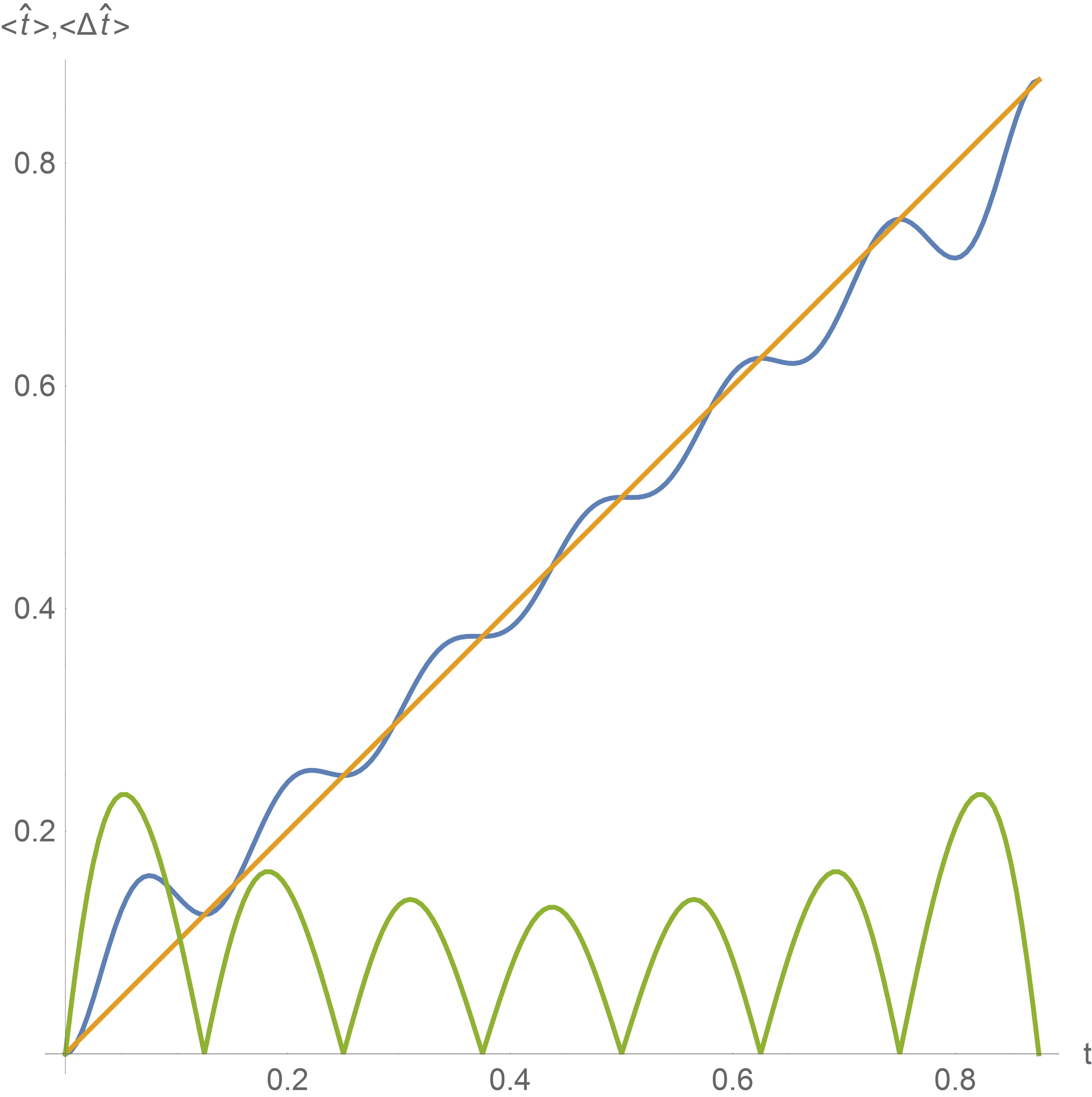
Figure 5: The expectation value (blue) and variance (green) of the time operator (449) given the initial state $\ket{\theta_{0}}$, for $d=8$, $T_{0}=1$. The idealised case $\braket{\hat{t}}=t$ is in orange.

A more fundamental shortcoming is that the time operator (449) can never approach the ideal commutation relation (436) with the Hamiltonian. As noted by Peres Peres ,

$$\braket{\theta_{k}}{[\hat{t}_{c},\hat{H}_{c}]}{\theta_{k}}=0,\quad\forall\,\,k\in{\mathbbm{Z}},\quad\forall\,\,d\in{\mathbbm{N}}^{+}.$$ (451)

This is consistent with the observation by H. Weyl Weyl that the canonical commutation relation cannot be obeyed by finite dimensional operators.

However, while the example of Eq. (451) demonstrates that ideal commutator is impossible to achieve for operators with domain on the full $d$ dimensional Hilbert space of the clock (even in the $d\rightarrow\infty$ limit), it is possible to approximately achieve this after one restricts the domain of the operators to a sub domain. The domain defined by the linear span of the clock states (Def. 1), which excludes pure angle states $\ket{\theta_{k}}$, is one such example, i.e.

$$[\hat{t}_{c},\hat{H}_{c}]\ket{\Psi}\approx i\ket{\Psi},$$ (452)

for clock states $\ket{\Psi}$, and where the approximation becomes exact in the $d\rightarrow\infty$ limit. In Section XI a rigorous version of Eq. (452) was derived.

Appendix C Mathematical results used in the proofs

There are many mathematical results used in the proof of this manuscript. Here we state the ones which are used repetitively in many proofs. When a mathematical result is used only once or twice; or confined to a particular lemma/theorem, it has been stated directly in the proof.

C.1 Fourier transform as a function of dimension $d$

Definition 12 (Standard fourier transform).

classicalfourieranalysis Given $f\in\ell({\mathbbm{R}})$ its Fourier transform is defined as

$$\bar{f}(\zeta)=\int_{{\mathbbm{R}}}f(x)e^{-i2\pi x\zeta}dx.$$ (453)

In this article, we do not use this version of the Fourier transform, rather we work extensively with the following Fourier transform with an additional parameter $d$,

Definition 13.

$$\tilde{\psi}(p)=\frac{1}{\sqrt{d}}\int_{{\mathbbm{R}}}\psi(x)e^{-i2\pi px/d}dx,$$ (454)

which is closely related to the Discrete Fourier transform.

Throughout the article, the words ‘Fourier transform’ and the shorthand $\mathcal{F}_{d}$ will refer to (454).

Corollary C.0.1 (Useful Fourier relations).

If $\mathcal{F}_{d}\left[\psi(x)\right]=\tilde{\psi}(p)$,

$$\psi(x)=\mathcal{F}^{-1}_{d}\left[\tilde{\psi}(p)\right] =\frac{1}{\sqrt{d}}\int_{-\infty}^{\infty}\tilde{\psi}(p)e^{+i2\pi px/d}dp$$ (455)

$$\mathcal{F}_{d}\left[\psi(x)e^{-i2\pi xa/d}\right] =\tilde{\psi}(p+a),$$ (456)

$$\mathcal{F}^{-1}_{d}\left[\tilde{\psi}(p)e^{i2\pi pb/d}\right] =\psi(x+b)$$ (457)

$$\mathcal{F}_{d}\left[x\psi(x)\right] =\left(\frac{id}{2\pi}\right)\frac{d}{dp}\tilde{\psi}(p),$$ (458)

$$\mathcal{F}^{-1}_{d}\left[p\tilde{\psi(p)}\right] =\left(-\frac{id}{2\pi}\right)\frac{d}{dx}\tilde{\psi}(x).$$ (459)

C.2 Poisson summation formula

We first present the formula for the case of the standard Fourier transform, and then modify it to the version we need.

Lemma C.0.1.

Suppose that a function $f$ and its (standard) Fourier transform $\bar{f}$ belong to $L^{1}({\mathbbm{R}}^{n})$ and satisfy

$$\left|f(x)\right|+\left|\bar{f}(x)\right|\leq C\left(1+x\right)^{-n-\delta}$$ (460)

for some $C,\delta>0$. Then $f$ and $\bar{f}$ are both continuous, and $\forall x\in{\mathbbm{R}}^{n}$ we have

$$\sum\limits_{m\in\mathbb{Z}^{n}}\bar{f}(m)=\sum\limits_{m\in\mathbb{Z}^{n}}f(m).$$ (461)

Note that any function in the Schwartz spaceclassicalfourieranalysis satisfies (460). In this article we use the Poisson summation only upon Gaussian functions or Gaussians multipled by functions of bounded derivatives, both of which are members of the Schwartz space.

Corollary C.0.2 (Poisson summation for $\mathcal{F}_{d}$).

If $\psi\in\ell({\mathbbm{R}})$,

$$\sum_{m\in\mathbb{Z}}\psi(m) =\sqrt{d}\sum_{m\in\mathbb{Z}}\tilde{\psi}(md),\text{ and }$$ (462)

$$\sum_{m\in\mathbb{Z}}\tilde{\psi}(m) =\sqrt{d}\sum_{m\in\mathbb{Z}}\psi(md).$$ (463)

C.3 Addition of errors

Lemma C.0.2.

(norm non-increasing errors add linearly) Consider a sequence of operators $\{\Delta_{m}\}_{m=1}^{N}$ on a finite dimensional Hilbert space $\mathcal{H}$ which are normalised or sub-normlaised w.r.t. the induced operator norm from the $l_{2}$ vector norm, i.e. $\|\Delta_{m}\|_{2}\leq 1$, and let $\{\ket{\Phi_{m}}\}_{m=0}^{N}$ be a sequence of (not necessarily normalised) pure states in $\mathcal{H}$ with the following property:

$$\left|\left|\,\ket{\Phi_{m}}-\Delta_{m}\ket{\Phi_{m-1}}\right|\right|_{2}=\epsilon_{m},$$ (464)

where $\|\cdot\|_{2}$ is the $l_{2}$ vector norm. Then $\forall\,n\in 1,2,3,\ldots,N$ we have

$$\left|\left|\,\ket{\Phi_{n}}-\Delta_{n}\Delta_{n-1}\ldots\Delta_{1}\ket{\Phi_{0}}\right|\right|_{2}\leq\sum_{m=1}^{n}\epsilon_{m}.$$ (465)

Proof.

By induction. The theorem is true by definition for $n=1$, and if the theorem is true for all $n$ up to $k$, then for $n=k+1$,

$$\left|\left|\;\ket{\Phi_{k+1}}-\Delta_{k+1}\Delta_{k}\ldots\Delta_{1}\ket{\Phi_{0}}\;\right|\right|_{2} =\left|\left|\;\ket{\Phi_{k+1}}-\Delta_{k+1}\ket{\Phi_{k}}+\Delta_{k+1}\left(\ket{\Phi_{k}}-\Delta_{k}\ldots\Delta_{1}\ket{\Phi_{0}}\right)\;\right|\right|_{2}$$ (466)

$$\leq\left|\left|\;\ket{\Phi_{k+1}}-\Delta_{k+1}\ket{\Phi_{k}}\;\right|\right|_{2}+\left|\left|\;\Delta_{k+1}\left(\ket{\Phi_{k}}-\Delta_{k}\ldots\Delta_{1}\ket{\Phi_{0}}\right)\;\right|\right|_{2}$$ (467)

$$\leq\left|\left|\;\ket{\Phi_{k+1}}-\Delta_{k+1}\ket{\Phi_{k}}\;\right|\right|_{2}+\left|\left|\Delta_{k+1}\right|\right|_{2}\,\left|\left|\;\left(\ket{\Phi_{k}}-\Delta_{k}\ldots\Delta_{1}\ket{\Phi_{0}}\right)\;\right|\right|_{2}$$ (468)

$$\leq\left|\left|\;\ket{\Phi_{k+1}}-\Delta_{k+1}\ket{\Phi_{k}}\;\right|\right|_{2}+\left|\left|\,\ket{\Phi_{k}}-\Delta_{k}\ldots\Delta_{1}\ket{\Phi_{0}}\right|\right|_{2}$$ (469)

$$=\epsilon_{k+1}+\sum_{m=1}^{k}\epsilon_{m}=\sum_{m=1}^{k+1}\epsilon_{m},$$ (470)

where we used the Minkowski vector norm inequality and the equivalence between the induced $l_{2}$ operator norm and the property $\|\Delta_{m}\|_{2}\leq 1$ in line (468).
∎

Appendix D A proof for the upper bound to $\tilde{\epsilon}_{V}$

Here we present a proof of Eq. (354); namely the inequality

$$\tilde{\epsilon}_{V}\leq\frac{(\pi-x_{vr})\mathrm{e}^{2}}{4\pi\sqrt{\pi}}\sqrt{n}\cos^{2n}(x_{vr}/2),\quad\text{if }\cos(x_{vr})\leq 1-\frac{1}{n}.$$ (471)

Proof.

From Eqs. (336) and (269) we find

$$\tilde{\epsilon}_{V} =\int_{x_{vr}-2\pi}^{x_{vl}}dxA_{c}\cos^{2n}\left(\frac{x}{2}\right)=A_{c}\left(\int_{x_{vr}-2\pi+2\pi}^{-\pi+2\pi}dx\cos^{2n}(x/2-\pi)-\int_{\pi}^{-x_{vl}}dx\cos^{2n}(-x/2)\right)$$ (472)

$$=2A_{c}\int_{x_{vr}}^{\pi}dx\cos^{2n}(x/2)=2A_{c}(\pi-x_{vr})\int_{0}^{1}dy\cos^{2n}\left((y\,x_{vr}+(1-y)\pi)/2\right).$$ (473)

We now note the convexity of the potential, namely on the interval $x\in(x_{vr},\pi)$,

$$\frac{d^{2}\;}{dx^{2}}\cos^{2n}(x/2)=\frac{n}{2}\cos^{2(n-1)}(x/2)\left(n(1-\cos(x))-1\right)\geq 0\implies\cos(x)\leq 1-\frac{1}{n},$$ (474)

thus noting that $\max_{x\in[x_{vr},\pi]}\cos(x)=\cos(x_{vr})$, it follows that $\cos^{2n}(x/2)$ is convex on $x\in[x_{vr},\pi]$ if $\cos(x_{vr})\leq 1-1/n$ and $\cos^{2n}\left((y\,x_{vr}+(1-y)\pi)/2\right)\leq y\cos^{2n}(x_{vr}/2)+(1-y)\cos^{2n}(\pi/2)=y\cos^{2n}(x_{vr}/2)$, $y\in[0,1]$. Hence using Eq. (472), we conclude

$$\tilde{\epsilon}_{V}\leq A_{c}(\pi-x_{vr})\cos^{2n}(x_{vr}/2),\quad\text{if }\cos(x_{vr})\leq 1-\frac{1}{n}.$$ (475)

Using Eq. (272) with $\Omega=1$ and Sterling’s formula, we find

$$A_{c}=\frac{2^{2n}}{2\pi\binom{2n}{n}}=\frac{2^{2n}}{2\pi}\frac{(n!)^{2}}{(2n)!}\leq\frac{\mathrm{e}^{2}}{4\pi\sqrt{\pi}}\sqrt{n},$$ (476)

thus giving us Eq. (354) (Eq. (471) above). ∎

Appendix E Error Bounds

E.1 The norm of a discretized Gaussian (Normalization of $\ket{\Psi(k_{0})}$)

In this section only, for simplicity, we further restrict the range of $\sigma\in(0,d)$ and $d$ to $\sigma\in[1,d)$ and $d=2,3,4,\ldots$.

E.1.1 Normalizing $\ket{\Psi(k_{0})}$

We calculate the norm of a state in the space $\Lambda_{\sigma,n_{0}}$:.

$$\left|\!\left|\ket{\Psi(k_{0})}\right|\!\right|_{2}^{2} =A^{2}\sum_{k\in\mathcal{S}_{d}(k_{0})}e^{-\frac{2\pi}{\sigma^{2}}(k-k_{0})^{2}}$$ (477)

$$=A^{2}\left(\sum_{k\in\mathbb{Z}}e^{-\frac{2\pi}{\sigma^{2}}(k-k_{0})^{2}}+\epsilon_{1}\right),$$ (478)

$$\text{where}\left|\epsilon_{1}\right| =\sum_{k\in\mathbb{Z}/\mathcal{S}_{d}(k_{0})}e^{-\frac{2\pi}{\sigma^{2}}(k-k_{0})^{2}}<\frac{2e^{-\frac{\pi d^{2}}{2\sigma^{2}}}}{1-e^{-\frac{2\pi d}{\sigma^{2}}}}:=\bar{\epsilon}_{1},$$ (479)

using results from Sec. E.2. Applying the Poissonian summation formula on the sum,

$$\left|\!\left|\ket{\Psi(k_{0})}\right|\!\right|_{2}^{2} =A^{2}\left(\frac{\sigma}{\sqrt{2}}\sum_{m\in\mathbb{Z}}e^{-\frac{\pi\sigma^{2}(md)^{2}}{2d^{2}}}e^{-i2\pi(md)k_{0}/d}+\epsilon_{1}\right)$$ (480)

$$=A^{2}\left(\frac{\sigma}{\sqrt{2}}+\epsilon_{2}+\epsilon_{1}\right),$$ (481)

$$\text{where}\left|\epsilon_{2}\right| \leq\frac{\sigma}{\sqrt{2}}\sum_{m\in\mathbb{Z}-\{0\}}e^{-\frac{\pi\sigma^{2}m^{2}}{2}}<\frac{\sigma}{\sqrt{2}}\,\frac{2e^{-\frac{\pi\sigma^{2}}{2}}}{1-e^{-\pi\sigma^{2}}}:=\bar{\epsilon}_{2}.$$ (482)

Thus for $\ket{\Psi_{\textup{nor}}(k_{0})}$ defined in Def. 1, we have that $A$ given by Eq. (25) satisfies

$$\left(\frac{2}{\sigma^{2}}\right)^{1/2}-\frac{\bar{\epsilon}_{1}+\bar{\epsilon}_{2}}{\frac{\sigma}{\sqrt{2}}\left(\frac{\sigma}{\sqrt{2}}+\bar{\epsilon}_{1}+\bar{\epsilon}_{2}\right)}\leq A^{2}\leq\left(\frac{2}{\sigma^{2}}\right)^{1/2}+\frac{\bar{\epsilon}_{1}+\bar{\epsilon}_{2}}{\frac{\sigma}{\sqrt{2}}\left(\frac{\sigma}{\sqrt{2}}-\bar{\epsilon}_{1}-\bar{\epsilon}_{2}\right)},$$ (483)

where $\bar{\epsilon}_{1}$, $\bar{\epsilon}_{2}$ are given by Eqs. (479) and (482) respectively. Note that since $\sigma\geq 1$, $d/\sigma\geq 2$, it follows that $\sigma/\sqrt{2}-\bar{\epsilon}_{1}-\bar{\epsilon}_{2}>0$ so that Eq. (483) has no singular points.

Of the two bounds $\bar{\epsilon}_{1}$ and $\bar{\epsilon}_{2}$, the first is the greater error for $\sigma>\sqrt{d}$, while the second dominates for $\sigma<\sqrt{d}$.

E.1.2 Re-normalizing $\ket{\Psi(k_{0})}$

In some instances we will have to re-normalize the state $\ket{\Psi(k_{0})}$. This will consist in upper bounding $A/A^{\prime}$ where both $A$ and $A^{\prime}$ satisfy Eq. (25) but for different values of $k_{0}$. We will thus want to upper bound

$$\epsilon_{\textit{A}}=\left|\frac{A}{A^{\prime}}-1\right|.$$ (484)

re-writing Eq. (483) using the short hand $a-\epsilon_{L}\leq A^{2}\leq a+\epsilon_{R}$, we can write

$$\epsilon_{\textit{A}}\leq\sqrt{\frac{a+\epsilon_{R}}{a-\epsilon_{L}}}-1=\sqrt{1+\frac{\epsilon_{L}+\epsilon_{R}}{a-\epsilon_{L}}}-1\leq\frac{\epsilon_{L}+\epsilon_{R}}{a-\epsilon_{L}}=\frac{2\sqrt{2}}{\sigma}\,\frac{\bar{\epsilon}_{1}+\bar{\epsilon}_{2}}{1-2(\bar{\epsilon}_{1}+\bar{\epsilon}_{2})/\sigma}<\frac{20\sqrt{2}}{3}\,\frac{\bar{\epsilon}_{1}+\bar{\epsilon}_{2}}{\sigma},$$ (485)

where in the last line we have converted back to the notation of Eq. (483) and simplified the expression. Recall that $\bar{\epsilon}_{1}$, $\bar{\epsilon}_{2}$ are given by Eqs. (479) and (482) respectively.

E.2 Bounds on the tails of discrete Gaussians

In this section we state some well known useful bounds which will be used throughout the proofs in appendix. For $\Delta\in{\mathbbm{R}}$, we have the following bounds on the summations over Gaussian tails.

Lemma E.0.1.

$$\sum_{n=a}^{\infty}e^{-\frac{(n-X)^{2}}{\Delta^{2}}}<\frac{e^{-\frac{(a-X)^{2}}{\Delta^{2}}}}{1-e^{-\frac{2(a-X)}{\Delta^{2}}}},\quad\text{for }a>X\in{\mathbbm{R}}$$ (486)

Proof.

$$\sum_{n=a}^{\infty}e^{-\frac{(n-X)^{2}}{\Delta^{2}}} =\sum_{m=0}^{\infty}e^{-\frac{(a-X+m)^{2}}{\Delta^{2}}}=e^{-\frac{(a-X)^{2}}{\Delta^{2}}}\sum_{m=0}^{\infty}e^{-\frac{2m(a-X)}{\Delta^{2}}}e^{-\frac{m^{2}}{\Delta^{2}}}$$ (487)

$$<e^{-\frac{(a-X)^{2}}{\Delta^{2}}}\sum_{m=0}^{\infty}e^{-\frac{2m(a-X)}{\Delta^{2}}}=\frac{e^{-\frac{(a-X)^{2}}{\Delta^{2}}}}{1-e^{-\frac{2(a-X)}{\Delta^{2}}}}$$ (488)

∎

Lemma E.0.2.

$$\sum_{n=a}^{\infty}(n-X)e^{-\frac{(n-X)^{2}}{\Delta^{2}}}<\left(a-X+\frac{\Delta^{2}}{2}\right)e^{-\frac{(a-X)^{2}}{\Delta^{2}}},\quad\text{for }a>X+\Delta\in{\mathbbm{R}}$$ (489)

Proof.

$$\sum_{n=a}^{\infty}(n-X)e^{-\frac{(n-X)^{2}}{\Delta^{2}}} =(a-X)e^{-\frac{(a-X)^{2}}{\Delta^{2}}}+\sum_{n=a+1}^{\infty}(n-X)e^{-\frac{(n-X)^{2}}{\Delta^{2}}}$$ (490)

Since $(x-X)e^{-\frac{(x-X)^{2}}{\Delta^{2}}}$ is monotonically decreasing for $x>X+\Delta$, (which $a$ satisfies),

$$\sum_{n=a+1}^{\infty}(n-X)e^{-\frac{(n-X)^{2}}{\Delta^{2}}}<\int_{a}^{\infty}(x-X)e^{-\frac{(x-X)^{2}}{\Delta^{2}}}dx=\frac{\Delta^{2}}{2}e^{-\frac{(a-X)^{2}}{\Delta^{2}}},$$ (491)

where we have used

$$\int_{b}^{\infty}xe^{-\frac{x^{2}}{\Delta^{2}}}dx=\frac{\Delta^{2}}{2}e^{-\frac{b^{2}}{\Delta^{2}}}.$$ (492)

∎

Lemma E.0.3.

$$\sum_{n=a}^{\infty}(n-X)^{2}e^{-\frac{(n-X)^{2}}{\Delta^{2}}}<\left((a-X)^{2}+\frac{\Delta^{2}}{2}\left(a-X+\frac{1}{1-e^{-\frac{2(a-X)}{\Delta^{2}}}}\right)\right)e^{-\frac{(a-X)^{2}}{\Delta^{2}}},\quad\text{for }a>X+\sqrt{2}\Delta\in{\mathbbm{R}}$$ (493)

Proof.

$$\sum_{n=a}^{\infty}(n-X)^{2}e^{-\frac{(n-X)^{2}}{\Delta^{2}}}=(a-X)^{2}e^{-\frac{(a-X)^{2}}{\Delta^{2}}}+\sum_{n=a+1}^{\infty}(n-X)^{2}e^{-\frac{(n-X)^{2}}{\Delta^{2}}}$$ (494)

Since $(x-X)^{2}e^{-\frac{(x-X)^{2}}{\Delta^{2}}}$ is monotonically decreasing for $x>X+\sqrt{2}\Delta$, (which $a$ satisfies),

$$\sum_{n=a+1}^{\infty}(n-X)^{2}e^{-\frac{(n-X)^{2}}{\Delta^{2}}} <\int_{a}^{\infty}(x-X)^{2}e^{-\frac{(x-X)^{2}}{\Delta^{2}}}dx$$ (495)

$$=\frac{\Delta^{2}}{2}\left((a-X)e^{-\frac{(a-X)^{2}}{\Delta^{2}}}+\int_{a}^{\infty}e^{-\frac{(x-X)^{2}}{\Delta^{2}}}dx\right)$$ (496)

We use the monotonicity again, together with lemma E.0.1,

$$\int_{a}^{\infty}e^{-\frac{(x-X)^{2}}{\Delta^{2}}}dx <\sum_{n=a}^{\infty}e^{-\frac{(n-X)^{2}}{\Delta^{2}}}<\frac{e^{-\frac{(a-X)^{2}}{\Delta^{2}}}}{1-e^{-\frac{2(a-X)}{\Delta^{2}}}}$$ (497)

∎

E.3 Commutator section

Here we provide some supplementary details to the proofs of some of the bounds used in the proof of Theorem XI.1.

1. Bounding $\quad\epsilon_{1}^{co}$

$$\left|\!\left|\ket{\epsilon_{1}^{co}}\right|\!\right|_{2} <T_{0}\sum_{k\in\mathcal{S}_{d}(k_{0}),k>\frac{d}{2}}\left|\psi(k_{0};k)\right|$$ (498)

$$<T_{0}\sum_{k=\frac{d+1}{2}}^{\infty}\left|\psi(k_{0};k)\right|$$ increasing the range of the sums (499)

$$<T_{0}\sum_{k=\frac{d}{2}}^{\infty}\left|\psi(k_{0};k)\right| \psi(k_{0};k)$$ monotonicity (decreasing) of (500)

$$<T_{0}\sum_{k=\frac{d}{2}}^{\infty}e^{-\frac{\pi d^{2}}{\sigma^{2}}(k-k_{0})^{2}}$$ (501)

$$<T_{0}A\frac{e^{-\frac{\pi}{\sigma^{2}}\left(\frac{d}{2}-k_{0}\right)^{2}}}{1-e^{-\frac{2\pi}{\sigma^{2}}\left(\frac{d}{2}-k_{0}\right)}}$$ (502)

$$=\begin{cases}\displaystyle 2T_{0}A\frac{e^{-\frac{\pi d}{4}(1-\beta)^{2}}}{1-e^{-\pi(1-\beta)}}&\mbox{if }\sigma=\sqrt{d}\\[10.0pt] \displaystyle 2T_{0}A\frac{e^{-\frac{\pi d^{2}}{4\sigma^{2}}(1-\beta)^{2}}}{1-e^{-\frac{\pi d}{\sigma^{2}}(1-\beta)}}&\mbox{otherwise}\end{cases}$$ (503)

2. Bounding $\quad\epsilon_{2}^{co}$

$$\left|\!\left|\ket{\epsilon_{2}^{co}}\right|\!\right|_{2} =\frac{T_{0}}{d\sqrt{d}}\sum_{n=0}^{d-1}\sum_{k\in\mathbb{Z}/\mathcal{S}_{d}(k_{0})}\left|k\psi(k_{0};k)\right|$$ (504)

$$<\frac{T_{0}}{\sqrt{d}}\sum_{k\in\mathbb{Z}/\mathcal{S}_{d}(k_{0})}\left|k\psi(k_{0};k)\right| n$$ trivial sum w.r.t. (505)

$$<\frac{2T_{0}A}{\sqrt{d}}\sum_{k=k_{0}+\frac{d}{2}}ke^{-\frac{\pi}{\sigma^{2}}(k-k_{0})^{2}}$$ picking the larger error (right side) (506)

$$<\frac{2T_{0}A}{\sqrt{d}}\sum_{k=k_{0}+\frac{d}{2}}\left[(k-k_{0})+k_{0}\right]e^{-\frac{\pi}{\sigma^{2}}(k-k_{0})^{2}}$$ splitting into two sums (507)

$$<\frac{2T_{0}A}{\sqrt{d}}\left[\frac{d}{2}+\frac{\sigma^{2}}{2\pi}+\frac{k_{0}}{1-e^{-\frac{2\pi}{\sigma^{2}}\frac{d}{2}}}\right]e^{-\frac{\pi}{\sigma^{2}}\left(\frac{d}{2}\right)^{2}}$$ (508)

$$<\begin{cases}\displaystyle T_{0}A\sqrt{d}\left(1+\frac{1}{\pi}+\frac{\beta}{1-e^{-\pi}}\right)e^{-\frac{\pi d}{4}}&\mbox{if }\sigma=\sqrt{d}\\[10.0pt] \displaystyle T_{0}A\sqrt{d}\left(1+\frac{\sigma^{2}}{\pi d}+\frac{\beta}{1-e^{-\frac{\pi d}{\sigma^{2}}}}\right)e^{-\frac{\pi d^{2}}{4\sigma^{2}}}&\mbox{otherwise}\end{cases}$$ (509)

3. Bounding $\quad\epsilon_{3}^{co}$

$$\left|\!\left|\ket{\epsilon_{3}^{co}}\right|\!\right|_{2} =\sqrt{d}\sum_{l\in\mathcal{S}_{d}(k_{0})}\sum_{n=0}^{d-1}\sum_{m\in\mathbb{Z}}\frac{A\sigma}{\sqrt{d}}\left|m\left(-\frac{2\pi\sigma^{2}}{d^{2}}(p-n_{0})-i\frac{2\pi k_{0}}{d}\right)e^{-\frac{\pi\sigma^{2}}{d^{2}}(p-n_{0})^{2}}\right|_{p=n+md}\ket{\theta_{l}}.$$ (510)

Trivial sum w.r.t. $l$, bound the error by twice the right side error (w.r.t. $m$), choose $n=-d/2$ for worst case scenario, then trivial sum over $n$, and express $n_{0}$ in terms of $\alpha$,

$$\left|\!\left|\ket{\epsilon_{3}^{co}}\right|\!\right|_{2} =2Ad^{2}\sigma 2\pi\sum_{m=1}^{\infty}\left[\left(m-\frac{1+\alpha}{2}\right)+\frac{1+\alpha}{2}\right]\left(\frac{\sigma^{2}}{d}\left(m-\frac{1+\alpha}{2}\right)+\frac{\beta}{2}\right)e^{-\pi\sigma^{2}\left(m-\frac{1+\alpha}{2}\right)^{2}}.$$ (511)

Applying all of the bounds on the tails of Gaussians on each of the 4 terms,

$$\frac{\left|\!\left|\ket{\epsilon_{3}^{co}}\right|\!\right|_{2}}{2\pi Ad^{2}} =2\sigma\cdot\frac{\sigma^{2}}{d}\left[\left(\frac{1-\alpha}{2}\right)^{2}+\frac{1}{2\pi\sigma^{2}}\left(\frac{1-\alpha}{2}+1+\frac{1}{1-e^{-\pi\sigma^{2}(1-\alpha)}}\right)\right]e^{-\frac{\pi\sigma^{2}}{4}(1-\alpha)^{2}}$$ (512)

$$+2\sigma\cdot\frac{\sigma^{2}}{d}\left(\frac{1+\alpha}{2}\right)\left(\frac{1-\alpha}{2}+\frac{1}{2\pi\sigma^{2}}\right)e^{-\frac{\pi\sigma^{2}}{4}(1-\alpha)^{2}}$$ (513)

$$+2\sigma\cdot\frac{\beta}{2}\left(\frac{1-\alpha}{2}+\frac{1}{2\pi\sigma^{2}}\right)e^{-\frac{\pi\sigma^{2}}{4}(1-\alpha)^{2}}$$ (514)

$$+2\sigma\cdot\left(\frac{1+\alpha}{2}\right)\frac{\beta}{2}\left(\frac{1}{1-e^{-\pi\sigma^{2}(1-\alpha)}}\right)e^{-\frac{\pi\sigma^{2}}{4}(1-\alpha)^{2}}$$ (515)

$$= \begin{cases}\displaystyle\sqrt{d}\left((1-\alpha)+\frac{1}{\pi d}\left(2+\frac{1}{1-e^{-\pi d(1-\alpha)}}\right)+\frac{\beta}{2}\left(1-\alpha+\frac{1}{\pi d}+\frac{1+\alpha}{1-e^{-\pi d(1-\alpha)}}\right)\right)e^{-\frac{\pi d}{4}(1-\alpha)^{2}}&\mbox{if }\sigma=\sqrt{d}\\[10.0pt] \displaystyle\sigma\left(\frac{\sigma^{2}}{d}(1-\alpha)+\frac{1}{\pi d}\left(2+\frac{1}{1-e^{-\pi\sigma^{2}(1-\alpha)}}\right)+\frac{\beta}{2}\left(1-\alpha+\frac{1}{\pi\sigma^{2}}+\frac{1+\alpha}{1-e^{-\pi\sigma^{2}(1-\alpha)}}\right)\right)e^{-\frac{\pi\sigma^{2}}{4}(1-\alpha)^{2}}&\mbox{otherwise}\end{cases}$$ (516)

4. Bounding $\quad\epsilon_{4}^{co}$

$$\left|\!\left|\ket{\epsilon_{4}^{co}}\right|\!\right|_{2} =\sum_{l\in\mathcal{S}_{d}(k_{0})}\sum_{m\in\mathbb{Z}/\{0\}}\left|\frac{d}{dx}\left(x\psi(k_{0};x)\right)\right|_{x=l+md}=\sum_{k\in\mathbb{Z}/\mathcal{S}_{d}(k_{0})}\left|\frac{d}{dx}\left(x\psi(k_{0};x)\right)\right|_{x=k}$$ (517)

$$=\sum_{k\in\mathbb{Z}/\mathcal{S}_{d}(k_{0})}\left|\left(1-\frac{2\pi}{\sigma^{2}}x(x-k_{0})+i\frac{2\pi n_{0}}{d}x\right)e^{-\frac{\pi}{\sigma^{2}}(x-k_{0})^{2}}\right|_{x=k}$$ (518)

Once again, bounding the error by twice the right side error (w.r.t. $m$), and expressing $k_{0}$ in terms of $\beta$,

$$\left|\!\left|\ket{\epsilon_{4}^{co}}\right|\!\right|_{2} <2dA\sum_{m=1}^{\infty}\left|1-\frac{2\pi}{\sigma^{2}}(k-k_{0})^{2}-\frac{2\pi}{\sigma^{2}}k_{0}(k-k_{0})+i\pi\alpha(k-k_{0}+k_{0})\right|e^{-\frac{\pi}{\sigma^{2}}(k-k_{0})^{2}}$$ (519)

Bounding each sum as a Gaussian tail, (first term is ignored as it will only make the total smaller, being of the opposite sign)

$$\left|\!\left|\ket{\epsilon_{4}^{co}}\right|\!\right|_{2} <2dA\frac{2\pi}{\sigma^{2}}\left(\frac{d^{2}}{4}+\frac{\sigma^{2}}{2\pi}\left(\frac{d}{2}+1+\frac{1}{1-e^{-\frac{\pi d}{\sigma^{2}}}}\right)\right)e^{-\frac{\pi d^{2}}{4\sigma^{2}}}$$ (520)

$$+2dA\frac{2\pi}{\sigma^{2}}\frac{\beta d}{2}\left(\frac{d}{2}+\frac{\sigma^{2}}{2\pi}\right)e^{-\frac{\pi d^{2}}{\sigma^{2}}}$$ (521)

$$+2dA\pi\alpha\left(\frac{d}{2}+\frac{\sigma^{2}}{2\pi}\right)e^{-\frac{\pi d^{2}}{\sigma^{2}}}$$ (522)

$$+2dA\pi\alpha\frac{\beta}{2}\frac{1}{1-e^{-\frac{\pi d}{\sigma^{2}}}}e^{-\frac{\pi d^{2}}{\sigma^{2}}}$$ (523)

$$<\begin{cases}\displaystyle dA\left(d(\pi+1)(1+\beta)+2+\frac{2}{1-e^{-\pi}}+\alpha\left(d(\pi+1)+\frac{\pi\beta}{1-e^{-\pi}}\right)\right)e^{-\frac{\pi d}{4}}&\mbox{if }\sigma=\sqrt{d}\\[10.0pt] \displaystyle dA\left(\left(\frac{\pi d^{2}}{\sigma^{2}}+d\right)(1+\beta)+2+\frac{2}{1-e^{-\frac{\pi d}{\sigma^{2}}}}+\alpha\left(\pi d+\sigma^{2}+\frac{\pi\beta}{1-e^{-\frac{\pi d}{\sigma^{2}}}}\right)\right)e^{-\frac{\pi d^{2}}{4\sigma^{2}}}&\mbox{otherwise}\end{cases}$$ (524)

ALTERNATE BOUND

$$\left|\!\left|\ket{\epsilon_{4}^{co}}\right|\!\right|_{2} =\sum_{l\in\mathcal{S}_{d}(k_{0})}\sum_{m\in\mathbb{Z}/\{0\}}\left|\frac{d}{dx}\left(x\psi(k_{0};x)\right)\right|_{x=l+md}$$ (525)

$$=\sum_{l\in\mathcal{S}_{d}(k_{0})}\sum_{m\in\mathbb{Z}/\{0\}}\left|\left(1-\frac{2\pi}{\sigma^{2}}x(x-k_{0})+i\frac{2\pi n_{0}}{d}x\right)e^{-\frac{\pi}{\sigma^{2}}(x-k_{0})^{2}}\right|_{x=l+md}$$ (526)

Once again, bounding the error by twice the right side error (w.r.t. $m$), and replacing $l$ by its worst case, and trivializing the sum w.r.t. $l$, and finally expressing $k_{0}$ in terms of $\beta$,

$$\left|\!\left|\ket{\epsilon_{4}^{co}}\right|\!\right|_{2} <2dA\sum_{m=1}^{\infty}\left|\left[1-\frac{2\pi d^{2}}{\sigma^{2}}\left(m-\frac{1}{2}\right)^{2}-\frac{2\pi d^{2}}{\sigma^{2}}\frac{\beta}{2}\left(m-\frac{1}{2}\right)+i2\pi d\frac{\alpha}{2}\left(m-\frac{1}{2}+\frac{\beta}{2}\right)\right]\right|e^{-\frac{\pi d^{2}}{\sigma^{2}}\left(m-\frac{1}{2}\right)^{2}}$$ (527)

Once again, bounding each sum as a Gaussian tail,

$$\left|\!\left|\ket{\epsilon_{4}^{co}}\right|\!\right|_{2} <2dA\frac{2\pi d^{2}}{\sigma^{2}}\left(\frac{1}{4}+\frac{\sigma^{2}}{2\pi d^{2}}\left(\frac{1}{2}+1+\frac{1}{1-e^{-\frac{\pi d^{2}}{\sigma^{2}}}}\right)\right)e^{-\frac{\pi d^{2}}{4\sigma^{2}}}$$ (528)

$$+2dA\frac{2\pi d^{2}}{\sigma^{2}}\frac{\beta}{2}\left(\frac{1}{2}+\frac{\sigma^{2}}{2\pi d^{2}}\right)e^{-\frac{\pi d^{2}}{\sigma^{2}}}$$ (529)

$$+2dA\pi d\alpha\left(\frac{1}{2}+\frac{\sigma^{2}}{2\pi d^{2}}\right)e^{-\frac{\pi d^{2}}{\sigma^{2}}}$$ (530)

$$+2dA\pi d\alpha\frac{\beta}{2}\frac{1}{1-e^{-\frac{\pi d^{2}}{\sigma^{2}}}}e^{-\frac{\pi d^{2}}{\sigma^{2}}}.$$ (531)

5. Bounding $\quad\epsilon_{5}^{co}$

$$\left|\!\left|\ket{\epsilon_{5}^{co}}\right|\!\right|_{2} =\frac{1}{\sqrt{d}}\sum_{n=0}^{d-1}\sum_{k\in\mathbb{Z}/\mathcal{S}_{d}(k_{0})}\left|\psi(k_{0};k)\right|,$$ (532)

$$=\sqrt{d}\sum_{k\in\mathbb{Z}/\mathcal{S}_{d}(k_{0})}e^{-\frac{\pi}{\sigma^{2}}(k-k_{0})^{2}} n$$ trivial sum w.r.t (533)

$$<2\sqrt{d}A\sum_{k-k_{0}=\frac{d}{2}}^{\infty}e^{-\frac{\pi}{\sigma^{2}}(k-k_{0})^{2}}$$ bound error by right side (534)

$$<\begin{cases}\displaystyle 2\sqrt{d}A\frac{e^{-\frac{\pi d}{4}}}{1-e^{-\pi}}&\mbox{if }\sigma=\sqrt{d}\\[10.0pt] \displaystyle 2\sqrt{d}A\frac{e^{-\frac{\pi d^{2}}{4\sigma^{2}}}}{1-e^{-\frac{\pi d}{\sigma^{2}}}}&\mbox{otherwise}\end{cases}$$ (535)

6. Bounding $\quad\epsilon_{6}^{co}$

$$\left|\!\left|\ket{\epsilon_{6}^{co}}\right|\!\right|_{2} <\frac{2\pi}{T_{0}}\sqrt{d}\sum_{l\in\mathcal{S}_{d}(k_{0})}\sum_{n=0}^{d-1}\sum_{m\in\mathbb{Z}}\left|m\tilde{\psi}(k_{0};n+md)\right|$$ (536)

Trivial sum w.r.t. $l$, bounding the error by the right side (w.r.t. $m$) and replacing $n$ by the worst case $n=-\frac{d}{2}$,

$$\left|\!\left|\ket{\epsilon_{6}^{co}}\right|\!\right|_{2} =\frac{2\pi}{T_{0}}d^{2}\sigma A\sum_{m=1}^{\infty}\left(\left(m-\frac{1+\alpha}{2}\right)+\frac{1+\alpha}{2}\right)e^{-\pi^{2}\sigma^{2}\left(m-\frac{1+\alpha}{2}\right)^{2}}$$ (537)

$$<\begin{cases}\displaystyle\frac{2\pi Ad^{2}\sqrt{d}}{T_{0}}\left(\frac{1-\alpha}{2}+\frac{1}{2\pi d}+\left(\frac{1+\alpha}{2}\right)\frac{1}{1-e^{-\pi d(1-\alpha)}}\right)e^{-\frac{\pi d}{4}(1-\alpha)^{2}}&\mbox{if }\sigma=\sqrt{d}\\[10.0pt] \displaystyle\frac{2\pi Ad^{2}\sigma}{T_{0}}\left(\frac{1-\alpha}{2}+\frac{1}{2\pi\sigma^{2}}+\left(\frac{1+\alpha}{2}\right)\frac{1}{1-e^{-\pi\sigma^{2}(1-\alpha)}}\right)e^{-\frac{\pi\sigma^{2}}{4}(1-\alpha)^{2}}&\mbox{otherwise}\end{cases}$$ (538)

7. Bounding $\quad\epsilon_{7}^{co}$

$$\left|\!\left|\ket{\epsilon_{7}^{co}}\right|\!\right|_{2} =\frac{d}{T_{0}}\sum_{l\in\mathcal{S}_{d}(k_{0})}\sum_{m\in\mathbb{Z}/\{0\}}\left|\frac{d}{dx}\psi(k_{0};x)\right|_{x=l+md}=\frac{dA}{T_{0}}\sum_{k\in\mathbb{Z}/\mathcal{S}_{d}(k_{0})}\left|\frac{d}{dx}\psi(k_{0};x)\right|_{x=k}$$ (539)

$$<\frac{2d}{T_{0}}\sum_{k-k_{0}=\frac{d}{2}}^{\infty}\left|\frac{2\pi}{\sigma^{2}}(k-k_{0})+i\frac{2\pi n_{0}}{d}\right|e^{-\frac{\pi}{\sigma^{2}}(k-k_{0})^{2}}$$ (540)

$$<\begin{cases}\displaystyle\frac{2\pi}{T_{0}}dA\left(1+\frac{1}{\pi}+\frac{\alpha}{1-e^{-\pi}}\right)e^{-\frac{\pi d}{4}}&\mbox{if }\sigma=\sqrt{d}\\[10.0pt] \displaystyle\frac{2\pi}{T_{0}}dA\left(\frac{d}{\sigma^{2}}+\frac{1}{\pi}+\frac{\alpha}{1-e^{-\frac{\pi d}{\sigma^{2}}}}\right)e^{-\frac{\pi d^{2}}{4\sigma^{2}}}&\mbox{otherwise}\end{cases}$$ (541)

8. Bounding $\quad\epsilon_{8}^{co}$

$$\left|\!\left|\ket{\epsilon_{8}^{co}}\right|\!\right|_{2} <dA\sum_{k=\frac{d}{2}}^{\infty}\left|\frac{2\pi}{\sigma^{2}}(k-k_{0})+i\frac{2\pi n_{0}}{d}\right|e^{-\frac{\pi}{\sigma^{2}}(k-k_{0})^{2}}$$ (542)

$$<\begin{cases}\displaystyle\pi dA\left(1-\beta+\frac{1}{\pi}+\frac{\alpha}{1-e^{-\pi(1-\beta)}}\right)e^{-\frac{\pi d}{4}(1-\beta)^{2}}&\mbox{if }\sigma=\sqrt{d}\\[10.0pt] \displaystyle\pi dA\left(\frac{d}{\sigma^{2}}(1-\beta)+\frac{1}{\pi}+\frac{\alpha}{1-e^{-\frac{\pi d}{\sigma^{2}}(1-\beta)}}\right)e^{-\frac{\pi d^{2}}{4\sigma^{2}}(1-\beta)^{2}}&\mbox{otherwise}\end{cases}$$ (543)

References

• (1) J. Howard. Molecular motors: structural adaptations to cellular functions. Nature, 389(6651):561–567, 1997.
• (2) Joachim Frank, editor. Molecular Machines in Biology. Cambridge University Press, 2011. Cambridge Books Online.
• (3) Shawn M. Douglas, Ido Bachelet, and George M. Church. A logic-gated nanorobot for targeted transport of molecular payloads. Science, 335(6070):831–834, 2012.
• (4) H. E. D. Scovil and E. O. Schulz-DuBois. Three-level masers as heat engines. Phys. Rev. Lett., 2:262–263, Mar 1959.
• (5) J. E. Geusic, E. O. Schulz-DuBios, and H. E. D. Scovil. Quantum equivalent of the carnot cycle. Phys. Rev., 156:343–351, Apr 1967.
• (6) N. Linden, S. Popescu, and P. Skrzypczyk. How small can thermal machines be? the smallest possible refrigerator. Physical review letters, 105(13):130401, 2010.
• (7) Jonatan Bohr Brask, Géraldine Haack, Nicolas Brunner, and Marcus Huber. Autonomous quantum thermal machine for generating steady-state entanglement. New Journal of Physics, 17(11):113029, 2015.
• (8) Fernando GSL Brandao, Michał Horodecki, Jonathan Oppenheim, Joseph M Renes, and Robert W Spekkens. Resource theory of quantum states out of thermal equilibrium. Physical review letters, 111(25):250404, 2013.
• (9) Artur SL Malabarba, Anthony J Short, and Philipp Kammerlander. Clock-driven quantum thermal engines. New Journal of Physics, 17(4):045027, 2015.
• (10) Friedemann Tonner and Günter Mahler. Autonomous quantum thermodynamic machines. Physical Review E, 72(6):066118, 2005.
• (11) David Gelbwaser-Klimovsky and Gershon Kurizki. Heat-machine control by quantum-state preparation: From quantum engines to refrigerators. Physical Review E, 90(2):022102, 2014.
• (12) Luis A Correa, José P Palao, Daniel Alonso, and Gerardo Adesso. Quantum-enhanced absorption refrigerators. Scientific reports, 4, 2014.
• (13) Friedemann Tonner and Günter Mahler. Quantum limit of the carnot engine. 1807–2007 Knowledge for Generations, 2007.
• (14) R. P. Feynman. The Feynman Lectures on Physics, volume 2. Addison-Wesley, 1963.
• (15) Noah Linden, Sandu Popescu, and Paul Skrzypczyk. How small can thermal machines be? the smallest possible refrigerator. Phys. Rev. Lett., 105:130401, Sep 2010.
• (16) P. Erker, Mitchison M.T., R. Silva, M. Woods, N. Brunner, and M. Huber. Autonomous quantum clocks: Does thermodynamics limit our ability to measure time? To appear in PRX.
• (17) J. E. Geusic, E. O. Schulz-DuBios, and H. E. D. Scovil. Quantum equivalent of the carnot cycle. Phys. Rev., 156:343–351, Apr 1967.
• (18) Fernando Brandão, Michał Horodecki, Nelly Ng, Jonathan Oppenheim, and Stephanie Wehner. The second laws of quantum thermodynamics. Proceedings of the National Academy of Sciences, 112(11):3275–3279, 2015.
• (19) W. van Dam and P. Hayden. Universal entanglement transformations without communication. Phys. Rev. A, 67(6):060302, June 2003.
• (20) V. Giovannetti, S. Lloyd, and L. Maccone. Advances in quantum metrology. Nat Photon, 5:222––229, 2011.
• (21) S. Ranković, TC. Liang, and R. Renner. Quantum clocks and their synchronisation - the alternate ticks game. 2015. arXiv:1506.01373v1.
• (22) Asher Peres. Measurement of time by quantum clocks. American Journal of Physics, 48(7), 1980.
• (23) V. Bužek, R. Derka, and S. Massar. Optimal quantum clocks. Phys. Rev. Lett., 82:2207–2210, Mar 1999.
• (24) Gordon R Allcock. The time of arrival in quantum mechanics i. formal considerations. Annals of physics, 53(2):253–285, 1969.
• (25) H. Salecker and E. P. Wigner. Quantum limitations of the measurement of space-time distances. Phys. Rev., 109:571–577, Jan 1958.
• (26) Max F Frenzel, David Jennings, and Terry Rudolph. Quasi-autonomous quantum thermal machines and quantum to classical energy flow. New Journal of Physics, 18(2):023037, 2016.
• (27) W. Pauli. Handbuch der Physik. Springer, Berlin, 24:83 – 272, 1933.
• (28) W. Pauli. Encyclopedia of Physics. Springer, Berlin, 1:60, 1958.
• (29) D. Gross, V. Nesme, H. Vogts, and R. F. Werner. Index theory of one dimensional quantum walks and cellular automata. Communications in Mathematical Physics, 310(2):419–454, Mar 2012.
• (30) Serge Massar and Philippe Spindel. Uncertainty relation for the discrete fourier transform. Phys. Rev. Lett., 100:190401, May 2008.
• (31) M. P. Woods, R. Silva, G. Pütz, S. R. Stupar, and R. Renner.
• (32) D. T. Pegg and S. M. Barnett. Phase properties of the quantized single-mode electromagnetic field. Phys. Rev. A, 39:1665–1675, Feb 1989.
• (33) P. Busch. No information without disturbance: Quantum limitations of measurement. In W.Myrvold J. Christian, editor, Quantum Reality, Relativistic Causality, and Closing the Epistemic Circle: An International Conference in Honour of Abner Shimony. Springer-Verlag, 2006. arXiv:0706.3526v1.
• (34) P. Busch. The time-energy uncertainty relation. Time in Quantum Mechanics, eds. J. G. Muga, R. Sala Mayato, I.L. Egusquiza, Springer-Verlag, Berlin (2002) pp. 69-98. 2nd rev. ed.
• (35) J. Åberg. Catalytic coherence. Phys. Rev. Lett., 113:150402, Oct 2014.
• (36) M. Abramonitz and I. Stegun. Handbook of Mathematical Functions with Formulas, Graphs, and Mathematical Tables.
• (37) G. Krantz, Steven and Harold R. Parks. A Primer of Real Analytic Functions. 2002.
• (38) Daniel Berend and Tamir Tassa. Improved bounds on bell numbers and on moments of sums of random variables. Probability and Mathematical Statistics, 30:185–205, 2010.
• (39) Lie Sophus and Engel Friedrich. Theorie der Transformationsgruppen. 1st edition, Leipzig; 2nd edition, AMS Chelsea Publishing, 1970, 1888.
• (40) J.C. Garrison and J. Wong. Canonically conjugate pairs, uncertainty relations, and phase operators. J. Math. Phys., 11:2242–2249, 1970.
• (41) M. Reed and B. Simon. Methods of Modern Mathematical Physics: Fourier analysis, self-adjointness. Number v. 2 in Methods of modern mathematical physics. Academic Press, 1975.
• (42) H. Weyl. Quantenmechanik und gruppentheorie. Zeitschrift für Physik, 46(1):1–46.
• (43) Loukas Grafakos. Classical Fourier Analysis. Springer, 2014.