Automatic Environmental Sound Recognition: Performance versus Computational Cost

Abstract

In the context of the Internet of Things (IoT), sound sensing applications are required to run on embedded platforms where notions of product pricing and form factor impose hard constraints on the available computing power. Whereas Automatic Environmental Sound Recognition (AESR) algorithms are most often developed with limited consideration for computational cost, this article seeks which AESR algorithm can make the most of a limited amount of computing power by comparing the sound classification performance as a function of its computational cost. Results suggest that Deep Neural Networks yield the best ratio of sound classification accuracy across a range of computational costs, while Gaussian Mixture Models offer a reasonable accuracy at a consistently small cost, and Support Vector Machines stand between both in terms of compromise between accuracy and computational cost.

I Introduction

Automatic speech recognition, music classification, audio indexing, and to a less visible extent biometric voice authentication, have now achieved some degree of commercial success in mass markets. A vast proportion of these applications are supported by PC platforms, cloud computing and powerful smartphones. Nevertheless, a new market is quickly emerging in the domain of the Internet of Things (IoT) [1]. In this market, Automatic Environmental Sound Recognition (AESR) [2] has a significant potential to create value, e.g., for security or home safety applications [3, 4, 5].

However, in this context, industrial reality imposes hard constraints on the available computing power. Indeed, IoT devices can be broadly divided into two classes: (a) devices which are perceived as “doing only one thing”, thus requiring the use of low cost processors to hit a price point that users are willing to pay for what the device does; (b) embedded devices where sound recognition comes as a bolt-on to add value to an existing product, for example adding audio analytic capabilities to a consumer grade camera or to a set-top box, thus requiring the algorithm to fit into the device’s existing design and price points. These two cases rule out the use of higher end processors. Generally speaking, the following features jointly define the financial cost of a processor and the level of constraint imposed on embedded computing: a) the clock speed is related to energy consumption; b) the instruction set is related to chip size and manufacturing costs, but in some cases includes special instruction sets to parallelise more operations into a single clock cycle; c) the architecture defines, e.g., the number of registers, number of cores, presence/absence of a Floating Point Unit (FPU), a Graphical Processing Unit (GPU) and/or a Digital Signal Processing (DSP) unit. These features affect applications in the obvious way of defining an upper limit on the number and the type of operations which can be executed in a given amount of time, thus ruling the possibility to achieve real time audio processing at the proportion of processor load allocated to the AESR application. Finally, onboard memory size is an important factor related to processor cost, as it affects both the computational performance, where repetitive operations can be cached to trade speed against memory, and the scalability of an algorithm, by imposing upper limits on the number of model parameters that can be stored and manipulated.

If trying to work within these limitations, and given that most IoT embedded devices allow Internet connectivity, it could be argued that cloud computing can solve the computational power constraints by abstracting the computing platform and making it virtually as powerful as needed. However, a number of additional design considerations may rule out the use of cloud computing for AESR applications: the latency introduced by cloud communications can be a problem for, e.g., time critical security applications [6]; regarding Quality of Service (QoS), network interruptions introduce an extra point of failure into the system; regarding privacy and bandwidth consumption, respectively, sending alerts rather than streaming audio or acoustic features out of the sound recognition device both rules out any possibility of eavesdropping [7] and requires less bandwidth.

Thus, the reality of embedded industrial applications is that at the price points acceptable in the marketplace, IoT devices will most likely be devoid of an FPU, will operate in the hundreds of Megahertz clock speed range, won’t offer onboard DSP or specialised instruction sets, and may prefer to run AESR on board rather than in the cloud. At the same time, most AESR performance evaluations are still produced with limited interest for the computational cost involved: many experimental results are obtained with floating point arithmetics on powerful computing platforms, and under the assumption that sufficient computing power will sooner or later become available for the algorithm to be practicable in the context of commercial applications.

This article aims at crossing this divide, by comparing the performance of three AESR algorithms as a function of their computational cost. In other terms, it seeks which AESR algorithm is able to make the most of a limited amount of computational power. The rest of the paper is organised as follows: Section II reviews prior art in AESR. Section III defines the measure of computational cost used in this study, and applies it to a range of popular machine learning algorithms. Section IV defines the other axis of this evaluation, which is the metric used to measure classification performance. The data sets and methodology are detailed in Section V, while results are discussed in Section VI.

II Background

Audio or sound recognition research has primarily been focused on speech and music signals. However in the past decade, the problem of classifying and identifying environmental sounds has received more attention [2]. AESR has applications in content-based search [8], robotics [9], security [3] and a host of other tasks. Recognition of environmental sounds is a part of the much broader field of computational auditory scene analysis (CASA) [10]. We are interested in the problem of identifying the presence of non-speech, non-music sounds or environmental sounds in a given audio recording. Environmental sound recognition involves the study of two closely related problems. Acoustic Scene Classification (ASC) involves selecting an appropriate set of labels that encompasses all the sound events which occur in a recording [11], e.g., “crowded train station”. With regards to machine learning, ASC can be seen as a sequence classification task where a set of labels is assigned to a variable length input sequence. A related problem is the problem of Acoustic Event Detection (AED). In addition to identifying the correct label, AED aims to segment the audio recording into regions where the label occurs [11], e.g., “stationmaster blowing whistle” or “doors closing”. Again with regards to machine learning, AED involves identifying the correct labels and the correct alignment of labels with the recording. In this study, we compare Gaussian mixture models (GMMs), support vector machines (SVMs) and deep neural networks (DNNs) in terms of their performance on an AED task as a function of their computational cost.

GMMs are generative probabilistic models and have been extensively applied to many problems in speech recognition [12]. In a number of cases, GMMs have therefore been considered a sensible starting point for research on the classification of environmental sounds. For example, they have been used to detect gunshot sounds [13] and to discriminate between gunshots and screams [14]. Portêlo et al. [15] have used Gaussian Mixtures as part of a hidden Markov model (HMM) approach to detecting sirens in audio. Elsewhere, Radhakrishnan et al. [16] have used GMMs when attempting to develop a model for recognising new ‘outlier’ sounds against a GMM trained to model background sounds. Principi et al. [17] proposed another novelty detection system, with an embedded implementation on a Beagle Board [18]. Atrey et al. [19] have used GMMs to classify audio frames into foreground or background sounds, then into vocal or nonvocal sounds and finally into ‘excited’ events (e.g. shouting, running) or ‘normal’ events (e.g. talking, walking).

SVMs are non-parametric classifiers that can generalise well given a limited training set and have well defined generalisation bounds [20]. Portêlo et al. [15] have experimented with an SVM when attempting to detect events in film audio. They found it to perform well on some sounds (aeroplanes, helicopters) but poorly on others (sirens, cats). By adding new features and applying PCA they found better performance on siren sounds. Moncrieff et al. [21] have also experimented with SVMs when attempting to classify sound events in film audio. Chen et al. [22] have used SVMs to classify audio data into music, speech, environmental sounds, speech mixed with music and environmental sounds mixed with music. Rouas et al. [23] have presented a comparison of SVMs and GMMs when attempting to detect shouting in public transport vehicles. Testing on audio recorded by actors on a train, they find that the SVM achieves a lower false alarm rate whilst the GMM seems better at making positive identifications.

More recently, Deep Learning, i.e., artificial neural networks with more than one intermediate hidden layer, have gained much popularity and have achieved impressive results on several machine learning tasks [24]. However, they do not seem to have been extensively applied to AESR so far. Toyoda et al. [25] have used a neural network to classify up to 45 different environmental sounds. They achieved high recognition accuracies, though it should be mentioned that both the training and test data sets used in their study may appear quite small in comparison to the data sets used nowadays as benchmarks for speech recognition and computer vision research. Baritelli et al. [26] used a DNN to classify 10 different environmental sounds. The authors found that the proposed system, which classified MFCCs directly, performed similarly to other AESR systems which were requiring more complex feature extraction. In [27], the authors used neural networks to estimate the presence or absence of people in a given recording, as well as the number of people and their proximity to the recording device. Gencoglu et al. [28] applied a deep neural network to an acoustic event detection task for classifying $61$ different classes of sounds. Their results showed this classifier to outperform a conventional GMM+HMM classification system.

Recently, the problem of AESR has been receiving more attention. Challenges like CLEAR [29] and DCASE [11] have been proposed in order to benchmark the performance of different approaches and to stimulate research. But, if drawing a parallel between the evolution of AESR and the evolution of speech recognition, the CLEAR and DCASE data sets could be thought of as being at the stage of the TIMIT era [30]: although the TIMIT data set was widely used for many years, it was limited in size to about 5.4 hours of speech data. The subsequent growth in the volume of available speech evaluation data sets has significantly contributed to bringing speech recognition to the levels of performance known today, where modern speech recognition systems are being trained over 1700 hours of data [31]. AED research is following a similar trend where the domain is now facing a need to collect larger data sets [32, 33] in order to make larger scale evaluations possible and to foster further technical progress.

Many studies explore feature learning to derive useful acoustic features that can be used to classify acoustic events [34, 35]. A limited number of publications apply k-Nearest Neighbours (k-NNs) [36, 37] or Random Forests [38] to AESR. However, these models have not been included in our comparative study, which is restricted to GMM, SVM and DNN models: these three types of models can be considered mainstream in terms of having been applied more extensively to a larger range of audio classification tasks which include speech, speaker and music classification and audio event detection. In preliminary experiments, we observed that k-NN classifiers were clearly outperformed by the classifiers included in this study.

III Computational cost

III-A Measure of computational cost used in this article

The fundamental question studied in this paper is that of comparing various machine learning algorithms as a function of their computational cost. A corollary to this question is to compare the rate of performance degradation that occurs when down-scaling various AESR algorithms by a comparable amount of computing operations: a given class of algorithms might be more resilient to down-scaling than another. While computational cost is related to computational complexity, both notions are distinct: computational cost simply counts the number of operations at a given model dimension, whereas computational complexity expresses the mathematical law according to which the computational cost scales up with the dimension of the input feature space.

Computational cost is studied here at the sound recognition stage, known as acoustic decoding. Unless specifically required by the application, it is indeed fairly rare to see the training stage of machine learning being realised directly on-board an embedded device. In most cases, it is possible to design the training as an offline process realised on powerful scientific computing platforms equipped with FPUs and GPUs. Offline training delivers a floating point model which is then quantised according to the needs of fixed point decoding in the embedded system [39]. It is generally accepted that the quantisation error introduced by this operation is unlikely to affect the acoustic modelling performance [40].

The computational cost estimate used in this study simply counts four types of basic operations: addition, comparison, multiplication, and lookup table retrieval (LUT). Multiply-add operations are commonly found in dot products, matrix multiplications and FFTs. Correlation operations, linear filtering or the Mahalanobis distance, at the heart of many recognition algorithms, rely solely on multiply-adds. Fixed point precision is fairly straightforward to manage over this type of operation. Divisions, on the other hand, and in particular matrix inversions, might be more difficult to manage. Regarding matrix inversion, it can happen that quantisation errors add up and make the matrix inversion algorithm unstable [41]. In many cases, it is possible to pre-compute the inversion of key parameters (e.g., variances), possibly offline and in floating point before applying fixed-point quantisation. Non-linear operations such as logarithms, exponentials, cosines, $N^{th}$ roots etc. are required by some algorithms. Two approaches can commonly be taken to transform non-linear functions into a series of multiply-adds: either Taylor series expansion, or look-up tables (LUTs). LUTs are more memory consuming than Taylor series expansions, but may require a lower number of instructions to achieve the desired precision. Generally speaking, it is important to be aware of the presence of a non-linearity in a particular algorithm, before assessing its cost: algorithms which rely on a majority of multiply-adds are more desirable than algorithms relying more heavily on non-linearities.

For all the estimates presented below, it is assumed that these four types of operations have an equal cost. While this assumption would be true for a majority of processors on the market, it may underestimate the cost of non-linear functions if interpolated LUTs or Taylor series are used instead of simpler direct LUT lookups. In addition to the 4 operations considered here, there are additional costs incurred with other operations (like data handling) in the processor. However, we use the simplifying assumption that the considered operations are running on the same core, thus minimizing data handling overhead.

As a case study, let us assume an attempt at running the K-nearest neighbours algorithm on a Cortex-M4 processor running at a clock speed of 80MHz and with 256kB of onboard memory. This is a very common hardware configuration for consumer electronic devices such as video cameras. Assuming that 20% of the processor activity is needed for general system tasks means that a maximum of 64 million of multiply or adds per second can be used for sound recognition ($80\mbox{MHz}\times 80\%=64\mbox{MHz}$). Assuming sound sampled at 16kHz and audio feature extracted at, e.g., a window shift of 256 samples, equivalent to 62.5 frames per second, means that the AESR algorithm should use no more than 1,024,000 multiply or adds per analysis frame (64MHz / 62.5Hz = 1 024K instructions).

From there, assuming a K-Nearest neighbour algorithm with a 40 dimensional observation vector $x$, mean vector $\mu$ and a Mahalanobis distance $(x-\mu)\sigma^{-1}(x-\mu)$ with a diagonal covariance matrix $\sigma$, there would be one subtraction and two multiplications per dimension for the Mahalanobis distance calculation, plus one operation for the accumulation across each dimension: four operations in total, thus entailing a maximum of 1,024,000 instructions / 4 operations / 40 dimensions = 6 400 nearest neighbours on this platform to achieve real-time recognition.

However, assuming that each nearest neighbour is a 40-dimensional vector of 32 bits/2 Bytes values, the memory requirement to store the model would be 512kB, which is double the 256kB available on the considered platform. Again assuming that the code size occupies 20% of the memory, leaving 80% of the memory for model storage, a maximum of $256\mbox{kB}\times 80\%\,/\,40\,\mbox{features}\,/\,2\mbox{Bytes}=2\,560$ nearest neighbours only which could be used as the acoustic model.

Depending on the choice of algorithm, memory is not always the limiting factor. In the case of highly non-linear algorithms, the computational cost of achieving real-time audio recognition might outweigh the model storage requirements. While only the final integration can tell if the desired computational load and precision are met, estimates can be obtained as illustrated in this case study in order to forecast if an algorithm will fit on a particular platform.

Feature	Addition	Multiplication	nonlinearity LUT lookup
GMM	$2(M\cdot(D+1)+M)$	$2M\cdot 2D$	$M$
SVM - Linear	$\lambda D+\lambda+1$	$\lambda\cdot D$	0
SVM - Polynomial	$\lambda D+\lambda+1$	$\lambda(D+d)$	0
SVM - Radial Basis Function	$2\lambda D+\lambda+1$	$\lambda(D+2)$	$\lambda$
SVM - Sigmoid	$\lambda D+\lambda+1$	$\lambda(D+1)$	$\lambda$
DNN - Sigmoid	$H\cdot(1+D+L+(L-1)H)+1$	$H\cdot(1+D+(L-1)H)$	$L\cdot H+1$
DNN - ReLU	$H\cdot(1+D+L+(L-1)H)+1$	$H\cdot(1+D+(L-1)H)$	$L\cdot H+1$
RNN - Tanh	$H\cdot(2+D+H+2(L-1)(H+1))+1$	$H\cdot(1+D+H+2(L-1)H)$	$L\cdot H+1$

TABLE I: Computational cost per frame of each compared AESR algorithm. $D$ is the dimensionality of the feature vector, $M$ is the number of Gaussian mixtures for a GMM. $\lambda$ is the number of support vectors for a SVM, $d$ is the degree of a polynomial kernel. For the neural networks: $H$ is the number of hidden units in each layer and $L$ is the number of layers.

III-B Computational cost estimates for the compared algorithms

Most AED systems use a common 3-step pipeline [11]. The audio recording is first converted into a time-frequency representation, usually by applying the short-time Fourier transform (STFT) to overlapping windows. This is followed by feature extraction from the time-frequency representation. Typically, Mel Frequency Cepstral Coefficients (MFCCs) have been used as standard acoustic features since the seventies, due to favourable properties when it comes to computing distances between sounds [42]. Then the acoustic features are input into an acoustic model to obtain a classification score, which in some cases is analogous to a posterior probability. The classification score is then thresholded in order to obtain a classification decision. Below, we provide an estimate of the computational cost for each of these operations.

Feature extraction - Engineering the right feature space for AESR is essential, since the definition of the feature space affects the separability of the classes of acoustic data. Feature extraction from sound recordings thus forms an additional step in the classification pipeline, which contributes to the overall computational cost. In this study, the GMMs, SVMs and DNNs are trained on a set of input features that are typically used for audio and speech processing (Section V-B). Although recent studies demonstrate that neural networks can be trained to jointly learn the features and the classifier [24], we have found that this method is impractical for most AESR problems where the amount of labelled data for training and testing is limited. Additionally, by training the different algorithms on the same set of features, we study the performance of the various classifiers as a function of computation cost, without having to account for the cost of extracting each type of feature from the raw audio waveform. It also allows a fair comparison of the discriminative properties of different classification algorithms on the same input feature space. Therefore, we factor out the computational cost of feature extraction.

Gaussian Mixture Models - Given a $D$ dimensional feature vector $x$, a GMM [43] is a weighted sum of Gaussian component densities which provides an estimate of the likelihood of $x$ being generated by the probability distribution defined by a set of parameters $\theta$:

$$p(x|\theta)=\sum\limits_{i=0}^{M-1}w_{i}\cdot g(x|\mu_{i},\Sigma_{i})$$ (1)

where:

$$g(x|\mu_{i},\Sigma_{i})=\frac{1}{(2\pi)^{\frac{D}{2}}|\Sigma_{i}|^{\frac{1}{2}}}\cdot e^{-\frac{1}{2}(x-\mu_{i})^{\prime}\Sigma_{i}^{-1}(x-\mu_{i})}$$ (2)

where $\theta=(\mu_{i},\Sigma_{i},w_{i})_{0\leq i<M}$ is the parameter set, $M$ is the number of Gaussian components, $\mu_{i}$ are the means, $\Sigma_{i}$ the covariance matrices and $w_{i}$ the weights of each Gaussian component. In practice, computing the likelihood in the log domain avoids numerical underflow. Furthermore, the covariance matrices are constrained to be diagonal, thus transforming equations (1) and (2) into:

$$\begin{array}[]{l}\log p(x|\theta)=\\ \;\;\textrm{logsum}_{i=0}^{M-1}\left\{\sum_{d=0}^{D-1}\left(x_{d}-\mu_{i,d}\right)^{2}\cdot\sigma_{i,d}^{-1}+w_{i}\right\}+K\end{array}$$ (3)

where $d$ is the dimension index, constant $K$ can be neglected for classification purposes, and logsum symbolises a recursive version of function $\log(a+b)=\log a+\log(1+e^{\left(\log b-\log a\right)})$ [44], which can be computed using a LUT on non-linearity $\log(1+e^{x})$. Calculating the log likelihood of a $D$-dimensional vector given a GMM with $M$ components therefore requires the following operations:

• $D$ subtractions (i.e., additions of negated means) and $2D$ multiplications per Gaussian to calculate the argument of the exponent.

• $1$ extra addition per Gaussian to apply the weight in the log domain.

• $M$ LUT lookups and $M$ additions for the non-linear logsum cumulation across the Gaussian components.

This leads to the computational cost per audio frame expressed in the first row of table I.

Support Vector Machines - Support Vector Machines (SVMs) [20] are discriminative classifiers. Given a set of data points belonging to two different classes, the SVM determines the optimal separating hyperplane between the two classes of data. In the linearly separable case, this is achieved by maximising the margin between two hyperplanes that pass through a number of support vectors. The optimal separating hyperplane is defined by all points x that satisfy:

$$\textrm{x}\cdot\textrm{w}+b=0$$ (4)

where w is a normal vector to the hyperplane and $\frac{|b|}{\|w\|}$ is the perpendicular distance from the hyperplane to the origin. Given that all data points $\textrm{x}_{i}$ satisfy:

$$\left\{\begin{array}[]{ll}\textrm{x}_{i}\cdot\textrm{w}+b\geq 1&\mbox{for labels $y_{i}=+1$}\\ \textrm{x}_{i}\cdot\textrm{w}+b\leq-1&\mbox{for labels $y_{i}=-1$}\end{array}\right.$$ (5)

It can be shown that the maximum margin is defined by minimising $\frac{\|\textrm{w}\|^{2}}{2}$. This can be solved using a Lagrangian formulation of the problem, thus producing the multipliers $\alpha_{i}$ and the decision function:

$$f(\textrm{x})=\textrm{sgn}\Big{(}\sum\limits_{i=0}^{N-1}y_{i}\alpha_{i}\textrm{x}\cdot\textrm{x}_{i}+b\Big{)}$$ (6)

where $N$ is the number of training examples and x is a feature vector we wish to classify. In practice, most of the $\alpha_{i}$ will be zero, and the $\textrm{x}_{i}$ for non-zero $\alpha_{i}$ are called the support vectors of the algorithm.

In the case where the data is not linearly separable, a non-linear kernel function $K(\textrm{x}_{i},\textrm{x}_{j})$ can be used to replace the dot products $\textrm{x}\cdot\textrm{x}_{i}$, with the effect of projecting the data into a higher dimensional space where it could potentially become linearly separable. The decision function then becomes:

$$f(\textrm{x})=\textrm{sgn}\Big{(}\sum\limits_{i=0}^{N-1}y_{i}\alpha_{i}K(\textrm{x},\textrm{x}_{i})+b\Big{)}$$ (7)

Commonly used kernel functions include:

$\bullet$ Linear:	$K(\textrm{x},\textrm{x}_{i})=\textrm{x}\cdot\textrm{x}_{i}$
$\bullet$ Polynomial:	$K(\textrm{x},\textrm{x}_{i})=(\textrm{x}\cdot\textrm{x}_{i})^{d}$
$\bullet$ Radial basis function (RBF):	$K(\textrm{x},\textrm{x}_{i})=\exp(-\gamma|\textrm{x}-\textrm{x}_{i}|^{2})$
$\bullet$ Sigmoid:	$K(\textrm{x},\textrm{x}_{i})=\tanh(\textrm{x}\cdot\textrm{x}_{i})$

A further refinement to the SVM algorithm makes use of a soft margin whereby a hyperplane can still be found even if the data is non-separable (perhaps due to mislabeled examples) [20]. The modified objective function is defined as follows:

$$\arg\min_{\textrm{w},\mathbf{\xi},b}\left\{\frac{1}{2}\|\textrm{w}\|^{2}+C\sum_{i=1}^{n}\xi_{i}\right\}$$ (8)

subject to: $y_{i}(\mathbf{w}\cdot\mathbf{x_{i}}-b)\geq 1-\xi_{i},\;\;\xi_{i}\geq 0$

$\xi_{i}$ are non-negative slack variables. The modified algorithm finds the best hyperplane that fits the data while minimising the error of misclassified data points. The importance of these error terms is determined by parameter $C$, which can control the tendency of the algorithm to over fit or under fit the data.

Given a support vector machine with $\lambda$ support vectors, a new $D$-dimensional example can be classified using $\lambda$ additions to sum the dot product results for each support vector, plus a further addition for the bias term. For each dot product, a support vector requires the computation of the kernel function, then $\lambda$ multiplications to apply the $\alpha_{i}$ multipliers.

Some kernels require a number of elementary operations, whereas others require a LUT lookup. Thus, depending on the kernel, the final costs are:

• SVM Linear – $(\lambda\cdot D)+\lambda+1$ additions and $(\lambda\cdot D)+\lambda$ multiplications.

• Polynomial – $\lambda(D+d+2)+1$ additions and $\lambda(D+2)$ multiplications, where $d$ is the degree of the polynomial.

• Radial Basis Function – $2\lambda D+\lambda+1$ additions, $\lambda(D+2)$ multiplications and $\lambda$ exponential functions.

• Sigmoid – $\lambda(D+2)+1$ additions and $\lambda(D+2)$ multiplications and $\lambda$ hyperbolic tangent functions.

The computational cost of SVMs per audio frame for these kernels is summarized in Table I.

Deep Neural Networks -

Two types of neural network architectures are compared in this study: Feed-Forward Deep Neural Networks (DNNs) and Recurrent Neural Networks (RNNs).

A Feed-Forward Deep Neural Network processes the input by a series of non-linear transformations given by:

$${h}^{i}=f\left({W}^{i}{h}^{i-1}+{b}^{i}\right)\;\mbox{for}\;0\leq i\leq L$$ (9)

where ${h}^{0}$ corresponds to the input $x$, ${W}^{i},{b}^{i}$ are the weight matrix and bias vector for the $i^{th}$ layer, and the output of the final layer ${h}^{L}$ is the desired output. The non-linearity $f$ in Equation 9 is usually a sigmoid $f(x)=1/\left(1+e^{-x}\right)$ or a hyperbolic tangent function $\tanh(x)$. However recent research in various domains has showed that the Rectified Linear Unit (ReLU) [45] non-linearity can lead to faster convergence of models during training. The ReLU function is defined as $f(x)=max(0,x)$, which is simpler than the sigmoid or $\tanh$ activation because it only requires a piecewise linear operator instead of a fixed point sigmoid or $\tanh$ LUT.

While feed forward networks are designed for stationary data, Recurrent Neural Networks (RNNs) are a class of neural networks designed for modelling temporal data. RNNs predict the output $y_{t}$ given an input $x_{t}$, at some time $t$ in the following way:

$${h}^{i}_{t}=f\left({W}^{i}_{f}{h}^{i-1}_{t}+{W}^{i}_{r}{h}^{i}_{t-1}+{b}^{i}\right)\;\mbox{for}\;0\leq i\leq L$$ (10)

where ${W}^{i}_{f},{W}^{i}_{r}$ are the forward and recurrent weight matrices for the $i^{th}$ recurrent layer, $b_{i}$ is bias for layer $i$, and $\theta=\left\{{W}^{i}_{f},{W}^{i}_{r},{b}^{i}\right\}_{0}^{L}$ are the model parameters. The input layer $h^{0}_{t}$ corresponds to the input $x_{t}$ and the output layer, $h^{L}_{t}$ corresponds to the output $y_{t}$. In Equation 10, $f$ is the hyperbolic tangent function. The choice of $f$ for the output layer depends on the particular modelling problem.

RNNs are characterised by the recurrent connections ${W}^{i}_{r}$ between the hidden units. Similar to feed forward neural networks, RNNs can have several recurrent layers stacked on top of each other to learn more complex functions [46]. Due to the recursive structure of the hidden layer, at any time $t$, the RNN makes a prediction conditioned on the entire sequence seen until time $t$: $y_{t}=f(x_{0}^{t})$.

For simplicity, every neural network in this study was constrained to have the same number $H$ of hidden units in each of its $L$ layers. The input dimensionality is denoted by $D$. The forward pass through a feed-forward neural network therefore involves the following computations:

• Multiplying a column vector of size $n$ with a matrix of size $n\times k$ involves $n\cdot k$ additions and an equal number of multiplication operations.

• Therefore the first layer involves $\left(D\cdot H\right)$ multiplication operations and $H\cdot\left(D+1\right)$ additions, where the additional $H$ additions are due to the bias term.

• The remaining $L-1$ layers involve the following computations: $\left(L-1\right)\cdot\left(H\cdot H\right)$ multiplications and $\left(L-1\right)\cdot\left(H\cdot(H+1)\right)$ additions.

• The output layer involves $H$ multiplications and $H+1$ additions.

• A non-linearity is applied to the outputs of each layer, leading to a total of $L\cdot H+1$ non-linearities.

• The RNN forward pass includes an additional matrix multiplication due to the recurrent connections. This involves $H\cdot H$ multiplications and an equal number of addition operations.

The computational cost estimates for DNNs and RNNs are summarised in Table I.

IV Performance metrics for sound recognition

Classification systems produce two types of errors: False Negatives (FN), a.k.a. Missed Detections (MD), i.e., target sounds which have not been detected, and False Positives (FP), a.k.a. False Alarms (FA), i.e., non-target sounds which have been mistakenly classified as the target sound [47]. Their correlates are the True Positives (TP), or correctly detected target sounds, and True Negatives (TN), or correctly rejected non-target sounds. In our experiments, “sounds” refer to feature frames associated with a particular sound class label. The above metrics are usually expressed as percentages of the available testing samples. They can be computed after an operating point or threshold has been selected [48] for a given classifier. Indeed, most classifiers output a real valued score, which can be, e.g., a log-likelihood ratio, a posterior probability or a distance. The binary target/non-target classification is then made by comparing the score to a threshold. Thus, a system can be made either more permissive, by choosing a threshold which lets through more True Positives at the expense of generating more False Positives, or the system can be made more conservative, if the threshold is set to filter out more False Positives at the expense of rejecting more sounds in general and thus generating more Missed Detections. For example, the operation point of a GMM classifier is defined by choosing a log-likelihood threshold.

Ideally, AESR systems should be compared independently of the choice of threshold. This can be achieved through the use of Detection Error Tradeoff (DET) curves [49], which depict the FA/MD compromises achieved across a sweep of operation points. DET curves are essentially equivalent to Receiver Operating Curves (ROC) [49], but plotted into normal deviate scale to linearise the curve, under the assumption that FA and MD scores are normally distributed. Given that the goal is to minimise the FA/MD compromises globally across all possible operation points, a DET curve closer to the origin means a better classifier. DET curve performance can thus be summarised for convenience into a single figure called the Equal Error Rate (EER), which is the point where the DET curve crosses the %FA = %MD diagonal line. In other terms, the EER represents the operation point where the system generates an equal rate of FA and MD errors.

For GMM based classification systems, the output score is the ratio between the likelihood of the target GMM and the likelihood of the universal background model (UBM): $P(x|\theta_{\mbox{\tiny target sound}})/P(x|\theta_{\mbox{\tiny UBM}})$ [43]. For neural networks, the output layer consists in a single unit followed by a sigmoid function, thus yielding a real-valued class membership probability $P(C=1|x)$ taken as the score value. For SVMs, the score can be defined as the argument of the $\textrm{sgn}()$ function in Equation 7: whereas the $\textrm{sgn}()$ function always amounts to classifying against a threshold fixed to zero, using its argument as a score suggests a more gradual notion of deviation from the margin defined by the support vectors, or in other terms it suggests a more gradual measure of belonging to one side or the other of the margin.

V Data sets and methodology

V-A Data sets

For the problem of AED, the training data set consists of audio recordings along with corresponding annotations or ground truth labels. The ground truth labels are usually provided in the form of alignments, i.e. onset times, offset times and the audio event labels. This is in contrast to ASC problems where the ground truth does not include alignments. ASC is similar to the problem of speech recognition where each recording has an associated word-level transcription. The alignments are then obtained as a by-product of the speech recognition model. For the problem of AED, annotating large quantities of data with onset and offset times requires significant effort from human annotators.

Historically, relatively small data sets of labelled audio have been used for evaluating AED systems. As a matter of fact, the two most popular benchmarks for AED algorithms known to date are the DCASE challenge [11] and the CLEAR challenge [29]. The DCASE challenge data provides 20 examples for each of the 16 event classes. While the data set for the CLEAR challenge contains approximately 60 training instances for each of the 13 classes. The typical approach to AED so far has been to extract features from the audio and then use a classifier or an acoustic model to classify the frames into event labels. Additionally, the temporal relationship between acoustic frames and outputs is modelled using HMMs [11].

In this study, we investigate whether a data-driven approach to AED can yield improved performance. Inspired by the recent success of Deep Learning [24], we investigate whether neural network acoustic models can outperform existing models when trained on sufficiently large data sets. Deep Neural Networks (DNNs) have recently contributed to significant progress in the fields of computer vision, speech recognition, natural language processing and other domains of machine learning. The superior performance of neural networks can be largely attributed to more computational power and the availability of large quantities of labelled data. Neural network models with millions of parameters can now be trained on distributed platforms to achieve good generalisation performance [50]. However, despite the strong motivation to use neural networks for various tasks, their application is limited by the availability of labelled data. For example, we trained many DNN architectures on the DCASE data, but were unable to beat the performance of a baseline GMM system.

In order to train large neural network models, we perform experiments using three private data sets made available by Audio Analytic Ltd. to support this study. These three data sets are subsets of much larger data collection campaigns led by Audio Analytic Ltd. to support the development of smoke alarm and baby cry detection products. Ground truth annotations with onset and offset times obtained from human annotators were also provided. The motivation for using these data sets is twofold. Firstly, to provide a large number of training and test examples for training models that recognize baby cries and smoke alarm sounds. Secondly, a very large world data set of ambient sounds is used as a source of impostor data for training and testing, in a way which emulates the quasi infinite prior probability of the system being exposed to non-target sounds instead of target ones. In other words, there are potentially thousands of impostor sounds which the system must reject in addition to identifying the target sounds correctly. While the DCASE challenge evaluates how an AED system performs at detecting one sound in the presence of 15 impostors or non-target sounds, the world data set allows to evaluate the performance of detecting smoke alarms or baby cries against the presence of over 1000 impostor sounds, in order to reflect a more realistic use case.

The Baby Cry data subset comprises a proportion of baby cries obtained from two different recording conditions: one through camcorder in a hospital environment, one through uncontrolled hand-held recorders in uncontrolled conditions (both indoors and outdoors). Each recording was from a different baby. The train/test split was done evenly, and set to achieve the same balance of both conditions in both the train and test set (about 3/4 hospital condition and 1/4 uncontrolled condition) without any overlap between sources for training and testing. The recordings in this data set sum up to $4\,822$ seconds of training data and $3\,669$ seconds of test data, from which $224\,076$ feature frames in the training set and $90\,958$ feature frames in the test set correspond to target baby cry sounds.

The Smoke Alarm data subset comprises recordings of 10 smoke alarm models, recorded through 13 different channels across 3 British homes. While it may be thought that smoke alarms are simple sounds, the variability associated with different tones, different audio patterns, different room responses and different channel responses does require some generalisation capability which either may not be available in simpler fingerprinting or template matching methods, or would require a very large database of templates. The training set comprises recordings from two of the homes, while the test set is composed of recordings from the remaining home. Thus, while the same device can appear in both the training and evaluation sets, the recording conditions are always different. So the results presented over the smoke alarm set focus mainly on the generalisation across room responses and recording conditions. The data set provided for this study consists of $15\,271$ seconds of training data and $5\,043$ seconds of testing data, of which $194\,142$ feature frames in the training set and $114\,753$ feature frames in the test set correspond to target smoke alarm sounds.

The World data set contains about 900 files covering 10 second samples of a wide variety of complex acoustic scenes recorded from numerous indoor and outdoor locations around the UK, across a wide and uncontrolled range of devices, and potentially covering more than a thousand sound classes. For example, a 10 seconds sample of “train station” scene from the world data set covers, e.g., train noise, speech, departure whistle and more, while a 10 second sample of “supermarket” covers babble noise, till beeps and children’s voices. While it does not seem feasible to enumerate all the specific classes from the World set, assuming that there are more than two classes per file across the 410 files reserved for testing leads to an estimate of more than a thousand classes in the test set. The 500 other files of the world set are used to train a non-target model, i.e., a Universal Background Model (UBM) [43] in the case of GMMs, or a negative input for neural network and SVM training. It was ensured that the audio files in the both the training and testing world sets were coming from completely disjoint recording sessions. The World data set provided for this study consists of $5\,000$ seconds of training data and $4\,089$ seconds of test data, thus amounting to $312\,500$ feature frames for training and $255\,562$ feature frames for testing.

Where necessary, the recordings were converted to 16kHz, 16 bits using a high quality resampling algorithm. No other pre-processing was applied to the waveform before feature extraction.

V-B Feature Extraction

For this experiment, Mel-frequency cepstral coefficient (MFCC) features were extracted from the audio. MFCC features are extensively used in speech recognition and in environmental sound recognition [13, 14, 15, 16]. In addition to MFCCs, the spectral centroid [13], spectral flatness [15], spectral rolloff [14], spectral kurtosis [14] and zero crossing rate [14, 19] were also computed. With audio sampled at 16kHz, all the features were calculated with a window size of $512$ samples and a hop size of $256$ samples. The first $13$ MFCCs were used for our experiments. Concatenating all the features thus lead to an $18$ dimensional feature vector of real values. Temporal information was included in the input representation by appending the first and second order differences of each feature. This led to an input representation with $18\times 3=54$ dimensions. It should be noted that the temporal difference features were used as inputs to all models except the RNNs, where only the $18$ dimensional features were used as inputs. This is due to the fact that the RNN is designed to make predictions conditioned on the entire sequence history (Equation 10). Therefore, explicitly adding temporal information to the inputs is unnecessary. The reduction in input dimensionality and related reduction in computational cost is offset by the extra weight matrix in the RNN (Table I). For all the experiments, the data was normalised to have zero mean and unit standard deviation, with the mean and standard deviation calculated over the entire training data independently for each feature dimension.

V-C Training Methodology

Gaussian Mixture Models - GMMs were trained using the expectation maximisation algorithm (EM) [51]. The covariance matrices were constrained to be diagonal. A grid search was performed to find the optimal number of Gaussians in the mixture, on the training set. The best model with number of components $M\in\{1,2,4,8,16,32,64,128,256,512,1024\}$ was used for evaluation. A validation set was created by randomly selecting 20% of the training data, while the remaining 80% of the data was used for parameter estimation. The model that performed the best on the validation set was later used for testing. All the Gaussians were initialised using the k-means++ algorithm [52]. A single UBM was trained on the World training data set. One GMM per target class was then trained independently of the UBM. We also performed experiments where GMMs for each class were estimated by adapting the UBM by Maximum A Posteriori (MAP) adaptation [53]. We observed that this method yielded inferior results. We also observed worse results when no UBM was used and class membership was determined by thresholding the outputs of individual class GMMs. In the following, results are therefore only reported for the best performing method, which is the likelihood ratio between independently trained UBM and target GMMs.

Support Vector Machines - The linear, polynomial, radial basis function (RBF) and sigmoid kernels were compared in our experiments. In addition to optimising the kernel parameters ($d,\gamma$), a grid search was performed over the penalty parameter $C$ (Equation 8). In practice, real-world data are often non-separable, thus a soft margin has been used as necessary. Model performance was estimated by evaluating performance on a validation set. The validation set was formed by randomly selecting 20% of the training data, while the remaining data was used for parameter estimation. Again, the best performing model on the validation set was used for evaluation. SVM training is known not to scale well to very large data sets [20]: it has a time-complexity of $O(T^{3})$, where $T$ is the number of training examples. As a matter of fact, our preliminary attempts at using the full training data sets led to prohibitive training times. Standard practice in that case is to down-sample the training set by randomly drawing $T$ frames from the target set, and the same number $T$ of frames from the world set as negative examples for training. Results presented in section VI with $T\in\left\{500,2000\right\}$ show that contrary to the intuitive thought that down-sampling might have disadvantaged the SVMs by reducing the amount of training data compared to the other machines, such data reduction actually improves SVM performance. As such, down-sampling can be thought of as an integral part of the training process, rather than as a reduction of the training data.

Deep Neural Networks - All neural network architectures were trained to output a distribution over the presence or absence of a class, using the backpropagation algorithm and stochastic gradient descent (SGD) [54]. The training data was divided into a $80/20$ training/validation split to find the optimum training hyper-parameters. All the target frames were used for each class, and an equal number of non-target frames was sampled randomly from the World data set, for both training and validation.

For the DNNs, a grid search was performed over the following parameters: number of hidden layers $L\in\left\{1,2,3,4\right\}$, number of hidden units per layer $H\in\left\{10,25,50,100,150\right\}$, hidden activations $act\in\left\{sigmoid,ReLU\right\}$. In order to minimise parameter tuning, we used ADADELTA [55] to adapt the learning rate over iterations. The networks were trained using mini-batches of size $100$ and training was accelerated using an NVIDIA Tesla K40c GPU. A constant dropout rate [56] of $0.2$ was used for all layers. The training was stopped if the cost on the validation set did not decrease after $20$ epochs.

For the RNNs, a grid search was performed over the following parameters: number of hidden layers $L\in\left\{1,2,3\right\}$ and number of hidden units per layer $H\in\left\{10,25,50,100,150\right\}$. An initial learning rate of $0.001$ was used and linearly decreased to $0$ over $1000$ iterations. A constant momentum rate of $0.9$ was used for all the updates. The training was stopped if the error on the validation set did not decrease after $20$ epochs. The training data was further divided into sub-sequences of length $100$ and the networks were trained on these sub-sequences without any mini-batching. Gradient clipping [57] was also used to avoid the exploding gradient problem in the early stages of RNN training. Clipping was triggered if the norm of the gradient update exceeded $10$.

VI Experimental results

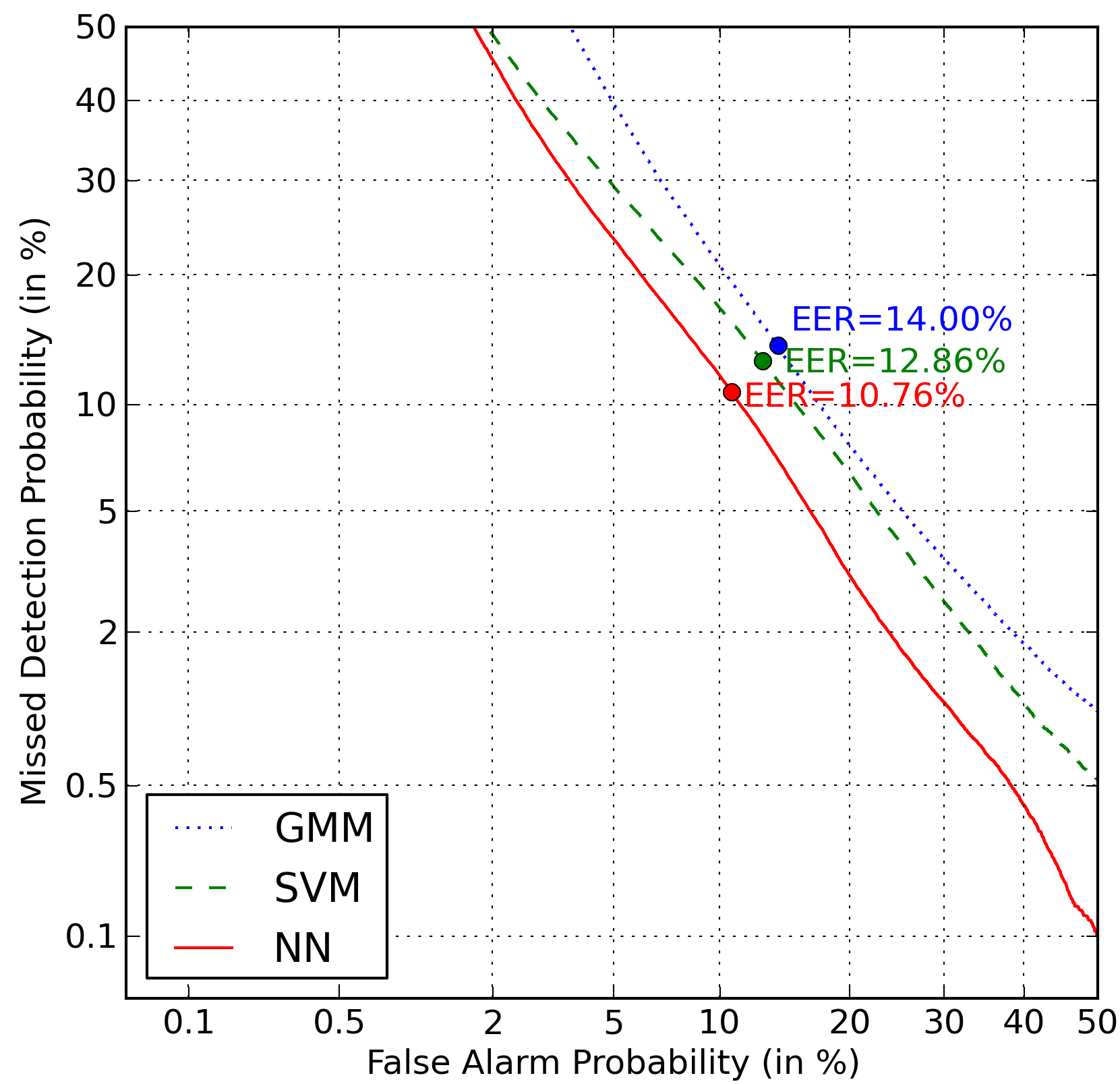
(a) Baby Cry data set

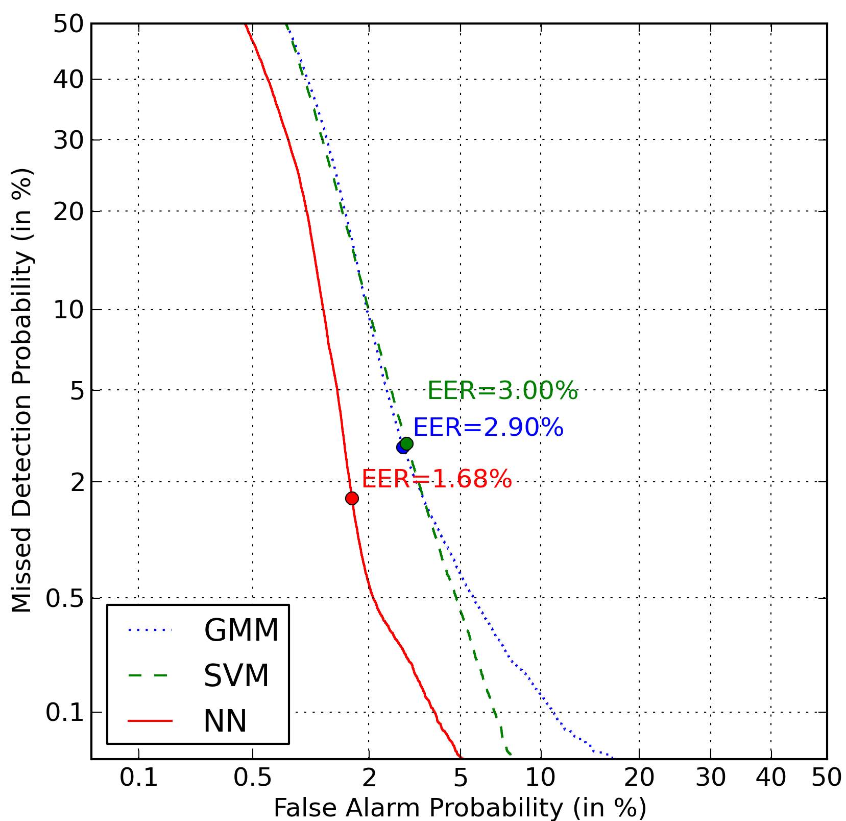
(b) Smoke Alarm data set

Figure 1: DET curves comparing frame classification performance of the acoustic classifiers.

Best Baby Cry classifiers	EER	# Ops.
GMM, $M=32$	14.0	10 560
Linear SVM, $T=2000$, $C=1.0$, $\lambda=655$	12.9	101 985
Feed-forward DNN, sigmoid, $L=2$, $H=50$	10.8	10 702

(a)

Best Smoke Alarm classifiers	EER	# Ops.
GMM, $M=16$	2.9	5 280
Linear SVM, $T=2000$, $C=0.1$, $\lambda=152$	3.0	46 655
Feed-forward DNN, sigmoid, $L=2$, $H=25$	1.7	4 102

(b)

TABLE II: Performance of the best classifiers on the Baby Cry and Smoke Alarm data sets.

In this section, classification performance is analysed for the task of recognising smoke alarms and baby cries against the large number of impostor sounds from the world set. Table II presents the EER for the best performing classifiers of each type and their associated computational cost. Figure 1 shows the corresponding DET curves. In Figure 2 we present a more detailed comparison between the performance of various classifier types against the computational cost involved in classifying a frame of input at test time.

Baby Cry data set - From Table IIa we observe that the best performing GMM has 32 components and achieves an EER of 14.0% for frame-wise classification. From Figure 2a (+ markers) we observe that there is no performance improvement when the number of Gaussian components is increased beyond 32. It should be noted that the best performing GMM (with $32$ components) has lower computational cost compared to any SVM classifier, and a cost comparable on average with DNN classifiers.

From Table IIa, we observe that a SVM with a linear kernel is the best performing SVM classifier, with an EER of $12.9\%$. The SVM was trained on 2000 examples, resulting in 655 support vectors. From Figure 2a, we note that the performance of the linear SVM (blue triangles) increases as the computational complexity (number of support vectors) is increased. The number of support vectors can also be controlled by varying the parameter $C$. For the best performing linear SVM, $C=1.0$ yields the best results. We observe that SVMs with a sigmoid kernel (light blue triangles) yield similar results to the linear SVM (Figure 2a). The best SVM with a sigmoid kernel yields an EER of 13.5%, while the second best sigmoid SVM has an EER of 13.9%. As in the linear case, we observe an improvement in test performance as the computational cost or the number of support vectors is increased.

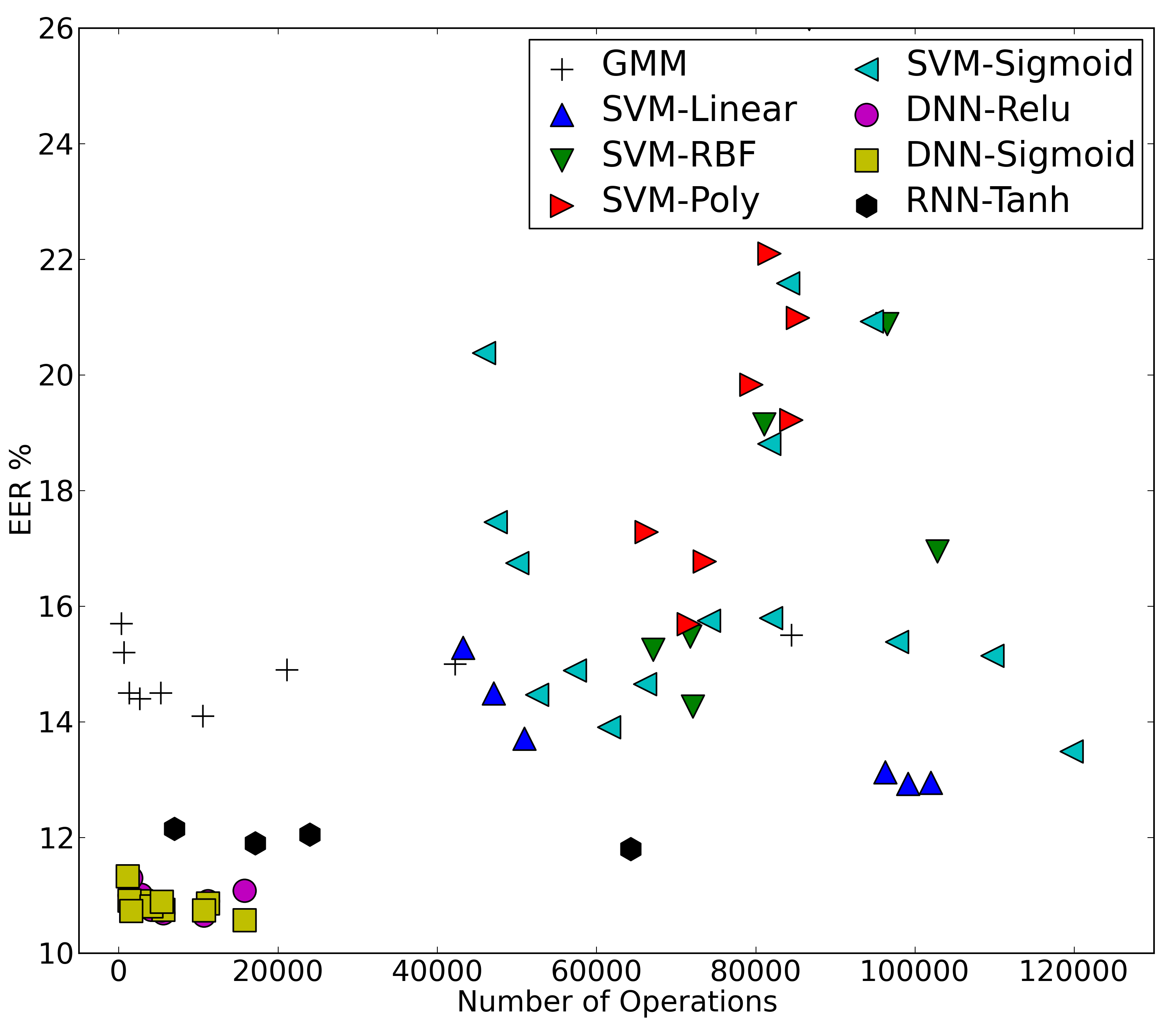
(a) Baby Cry Data set

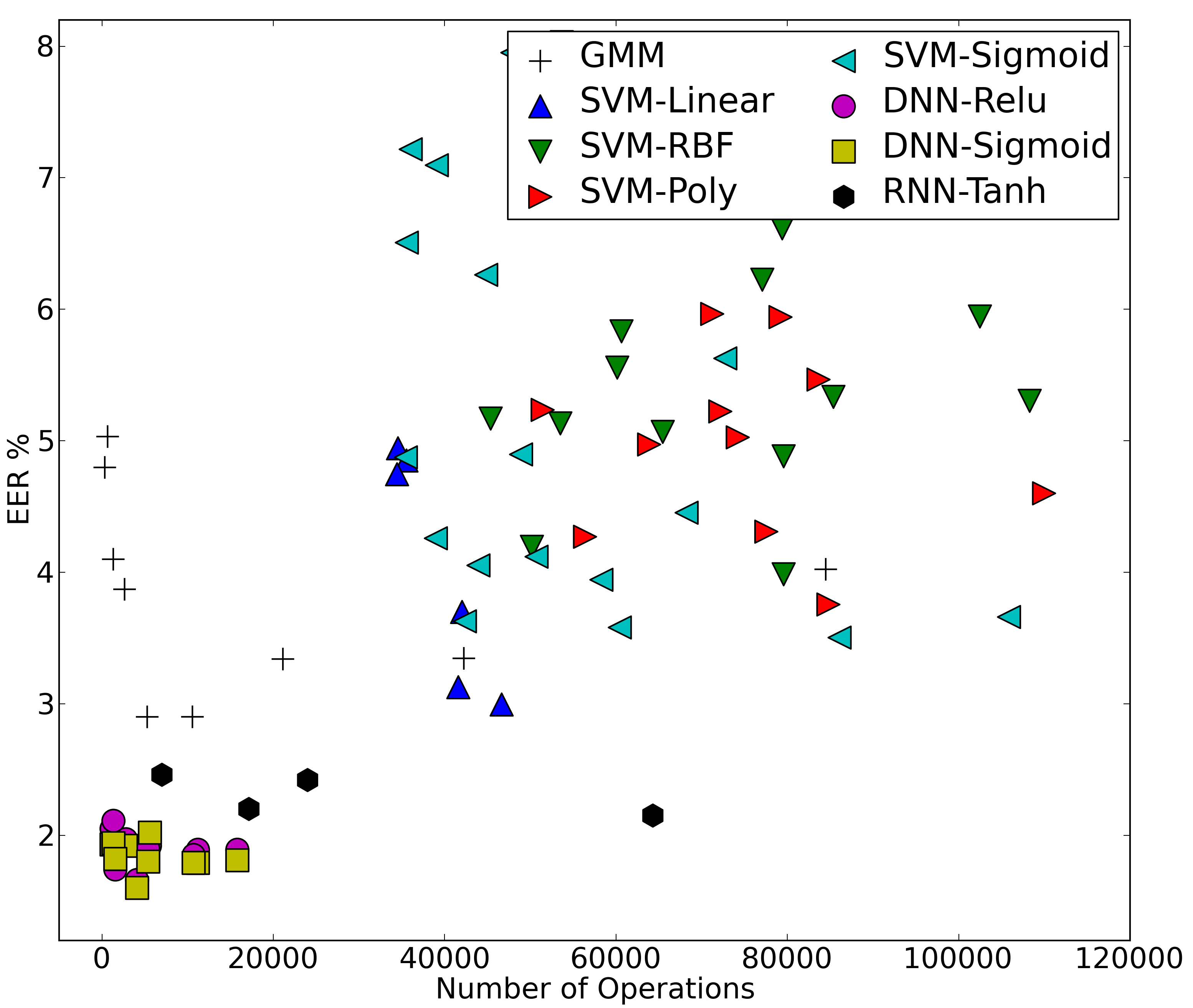
(b) Smoke Alarm Data set

Figure 2: Acoustic frame classification performance (EER percentage) as a function of the number of operations per frame, for each of the tested models, across the Baby Cry and Smoke Alarms data sets.

From Figure 2a, we note that SVMs with RBF and polynomial kernels (green and red triangles) are outperformed by linear and sigmoid SVMs, both in terms of %EER and computational cost. There is also no observable trend between test performance and computational cost. For the polynomial SVM (red triangles), we found a kernel with $d=3$ yielded the best performance, while low values of gamma $\gamma\in(0.005,0.01)$ provided the best results for the RBF kernel (Section III-B).

The number of training examples $T=2000$ was empirically determined to be the optimal value: adding more training examples did not yield any improvement in performance. Conversely, we tried training the same classifiers with $T=500$ training examples, since the computational cost of SVMs is determined both by the type of kernel and the number of support vectors, the latter being controlled by varying the number of training examples and the penalty parameter $C$. With $T=500$ and $C=0.1$, we were able to achieve a minimum EER rate of $13.7\%$ with the linear SVM, while halving the number of operations.

From Table IIa, the best performing neural network architecture, which achieves an EER of $10.8\%$, is a feed-forward DNN with sigmoid activations for the hidden units. Figure 1a shows that the neural network clearly outperforms all the other models. From Figure 2a we observe that the feed forward DNNs (circle and square markers) achieve similar test performance over a wide range of computational costs. This demonstrates that the network performance is not particularly sensitive to the specific number of hidden units in each layer. However, we did observe that networks which were deeper ($>1$ hidden layer) yielded better performance. From Figure 2a, we observe that the RNN architectures (hexagonal markers) yield slightly worse performance and are computationally more expensive. An interesting observation from Figure 2a is that feed-forward DNNs with both sigmoid and ReLU activations yield similar results. This is a very important factor when deploying these models on embedded hardware, since a ReLU net can be implemented with only linear operations (multiplications and additions), without the need for costly Taylor series expansions or LUTs.

Smoke Alarm data set - From Table IIb, we observe that the best performing GMM yields an EER of 2.9% and uses 16 mixture components. From Figure 2b (+ markers), we observe that the GMM performance improves as the computation cost (number of Gaussians) increases till $M=32$. Beyond this, increasing the number of Gaussian components does not improve results. Again, we observe that the best performing GMM with $M=32$ has much lower computational cost compared to SVMs, and a cost comparable on average with DNNs.

Similar to the results on the Baby Cry data set, the linear and sigmoid kernel SVMs show the best performance, out of all four SVM kernel types. The best linear SVM has an EER of 3.0% – a small improvement over the best GMM approach, but with a small increase in the number of operations. The model used 2000 training examples and $C=1.0$. From Figure 2b we again observe an improvement in performance, with an increase in computation cost for both the linear and sigmoid kernels (blue triangles). The best sigmoid kernel SVM scored 3.5% with 2000 training examples, while another configuration scored 3.6% with $T=500$ and $C=1$, at half the number of operations. Again, the polynomial and RBF kernels (red and green triangles) yield lower performance, with no observable trend in terms of performance versus computational cost (Figure 2b).

From Table IIb, we observe that a feed-forward sigmoid DNN yields the best performance, with an EER of $1.6\%$. From the DET curves (Figure 1b), we see that the neural network clearly outperforms the other models. From figure 2b we note that the neural networks consistently perform better than the other models, over a wide range of computational costs, which correspond to different network configurations (number of layers, number of units in each layer). The ReLU networks perform similarly to the sigmoid networks, while the RNNs perform worse and are computationally more costly.

It is worth noting that the performance of all classifiers is significantly better for the smoke alarm sounds, since the smoke alarms are composed of simple tones. On the other hand, baby cries have a large variability and are therefore more difficult to classify.

VII Conclusion

In this study, we compare the performance of neural network acoustic models with GMMs and SVMs on an environmental audio event detection task. Unlike other machine learning systems, AESR systems are usually deployed on embedded hardware, which imposes many computational constraints. Keeping this in mind, we compare the performance of the models as a function of their computational cost. We evaluate the models on two tasks, detecting baby cries and detecting smoke alarms against a large number of impostor sounds. These data sets are much larger than the popular data sets found in AESR literature, which enables us to train neural network acoustic models. Additionally, the large number of impostor sounds allows to investigate the performance of the proposed models in a testing scenario that is closer to practical use cases than previously available data sets.

Results suggest that GMMs provide a low cost baseline for classification, across both data sets. The GMM acoustic models are able to perform reasonably well at a modest computational cost. SVMs with linear and sigmoid kernels yield similar EER performance compared to GMMs, but their computational cost is overall higher. The computational cost of the SVM is determined by the number of support vectors. Unlike GMMs, SVMs are non-parametric models which do not allow the direct specification of model parameters, although the number of support vectors can be indirectly controlled with regularisation. Finally, our results suggest that deep neural networks consistently outperform both the GMMs and the SVMs on both data sets. The computational cost of DNNs can be controlled by limiting the number of hidden units and the number of layers. While changes in the number of units in the hidden layers did not appear to have a large impact on performance, deeper networks appeared to perform better in all cases. Additionally, neural networks with ReLU activations achieved good performance, while being an attractive choice for deployment on embedded devices because they do not require expensive LUT lookup operations.

In the future, we would like to expand the evaluations presented here to include more event classes. However, the lack of large data sets for AESR problems is a major limitation. We hope that studies like this one will encourage collaboration with industry partners to collect large data sets for more rigorous evaluations. We would also like to investigate the performance of acoustic models as a function of the memory efficiency, since memory is an important consideration when designing models for embedded hardware.

VIII Acknowledgements

The authors would like to thank the three anonymous reviewers whose comments helped to improve the article.

This work was supported by funding from Innovate UK, EPSRC grants EP/M507088/1 & EP/N014111/1 from the UK Engineering and Physical Sciences Research Council, as well as private funding from Audio Analytic Ltd.

References

- [1] J. Gubbi, R. Buyya, S. Marusic, and M. Palaniswami, “Internet of Things (IoT): A vision, architectural elements, and future directions,” Future Generation Computer Systems, vol. 29, no. 7, pp. 1645–1660, 2013.
- [2] S. Chachada and C.-C. J. Kuo, “Environmental sound recognition: A survey,” APSIPA Transactions on Signal and Information Processing, vol. 3, p. e14, 2014.
- [3] D. Istrate, E. Castelli, M. Vacher, L. Besacier, and J.-F. Serignat, “Information extraction from sound for medical telemonitoring,” IEEE Transactions on Information Technology in Biomedicine, vol. 10, no. 2, pp. 264–274, 2006.
- [4] M. Vacher, F. Portet, A. Fleury, and N. Noury, “Challenges in the processing of audio channels for ambient assisted living,” in Proceedings of the 12th IEEE International Conference on e-Health Networking Applications and Services (Healthcom), 2010. IEEE, 2010, pp. 330–337.
- [5] R. Sitte and L. Willets, “Non-speech environmental sound identification for surveillance using self-organizing-maps,” in Proceedings of the Fourth conference on IASTED International Conference: Signal Processing, Pattern Recognition, and Applications. ACTA Press, 2007, pp. 281–286.
- [6] F. Bonomi, R. Milito, P. Natarajan, and J. Zhu, “Fog computing: A platform for internet of things and analytics,” in Big Data and Internet of Things: A Roadmap for Smart Environments. Springer, 2014, pp. 169–186.
- [7] C. M. Medaglia and A. Serbanati, “An overview of privacy and security issues in the internet of things,” in The Internet of Things. Springer, 2010, pp. 389–395.
- [8] T. Virtanen and M. Helén, “Probabilistic model based similarity measures for audio query-by-example,” in IEEE Workshop on Applications of Signal Processing to Audio and Acoustics. IEEE, 2007, pp. 82–85.
- [9] N. Yamakawa, T. Takahashi, T. Kitahara, T. Ogata, and H. G. Okuno, “Environmental sound recognition for robot audition using matching-pursuit,” in Modern Approaches in Applied Intelligence. Springer, 2011, pp. 1–10.
- [10] D. Wang and G. J. Brown, Computational auditory scene analysis: Principles, algorithms, and applications. Wiley-IEEE Press, 2006.
- [11] D. Stowell, D. Giannoulis, E. Benetos, M. Lagrange, and M. D. Plumbley, “Detection and classification of acoustic scenes and events,” IEEE Transactions on Multimedia, vol. 17, no. 10, pp. 1733–1746, 2015.
- [12] L. Rabiner and B.-H. Juang, Fundamentals of speech recognition. Prentice Hall, 1993.
- [13] C. Clavel, T. Ehrette, and G. Richard, “Events detection for an audio-based surveillance system,” in IEEE International Conference on Multimedia and Expo (ICME). IEEE, 2005, pp. 1306–1309.
- [14] G. Valenzise, L. Gerosa, M. Tagliasacchi, E. Antonacci, and A. Sarti, “Scream and gunshot detection and localization for audio-surveillance systems,” in IEEE Conference on Advanced Video and Signal Based Surveillance (AVSS). IEEE, 2007, pp. 21–26.
- [15] J. Portelo, M. Bugalho, I. Trancoso, J. Neto, A. Abad, and A. Serralheiro, “Non-speech audio event detection,” in IEEE International Conference on Acoustics, Speech and Signal Processing (ICASSP). IEEE, 2009, pp. 1973–1976.
- [16] R. Radhakrishnan, A. Divakaran, and P. Smaragdis, “Audio analysis for surveillance applications,” in IEEE Workshop on Applications of Signal Processing to Audio and Acoustics. IEEE, 2005, pp. 158–161.
- [17] E. Principi, S. Squartini, R. Bonfigli, G. Ferroni, and F. Piazza, “An integrated system for voice command recognition and emergency detection based on audio signals,” Expert Systems with Applications, vol. 42, no. 13, pp. 5668 – 5683, 2015. [Online]. Available: http://www.sciencedirect.com/science/article/pii/S0957417415001438
- [18] R. Bonfigli, G. Ferroni, E. Principi, S. Squartini, and F. Piazza, “A real-time implementation of an acoustic novelty detector on the BeagleBoard-xM,” in 6th European Embedded Design in Education and Research Conference (EDERC), Sept 2014, pp. 307–311.
- [19] P. K. Atrey, M. Maddage, and M. S. Kankanhalli, “Audio based event detection for multimedia surveillance,” in IEEE International Conference on Acoustics, Speech and Signal Processing., vol. 5. IEEE, 2006.
- [20] C. J. Burges, “A tutorial on support vector machines for pattern recognition,” Data Mining and Knowledge Discovery, vol. 2, no. 2, pp. 121–167, 1998.
- [21] S. Moncrieff, C. Dorai, and S. Venkatesch, “Detecting indexical signs in film audio for scene interpretation,” in IEEE International Conference on Multimedia and Expo (ICME)., Aug 2001, pp. 989–992.
- [22] L. Chen, S. Gunduz, and M. T. Ozsu, “Mixed type audio classification with support vector machine,” in IEEE International Conference on Multimedia and Expo (ICME). IEEE, 2006, pp. 781–784.
- [23] J.-L. Rouas, J. Louradour, and S. Ambellouis, “Audio events detection in public transport vehicle,” in IEEE Intelligent Transportation Systems Conference (ITSC). IEEE, 2006, pp. 733–738.
- [24] Y. LeCun, Y. Bengio, and G. Hinton, “Deep learning,” Nature, vol. 521, no. 7553, pp. 436–444, 2015.
- [25] Y. Toyoda, J. Huang, S. Ding, and Y. Liu, “Environmental sound recognition by multilayered neural networks,” in The 4th International Conference on Computer and Information Technology (CIT). IEEE, 2004, pp. 123–127.
- [26] F. Beritelli and R. Grasso, “A pattern recognition system for environmental sound classification based on MFCCs and neural networks,” in Proceedings of the 2nd International Conference on Signal Processing and Communication Systems (ICSPC). IEEE, 2008.
- [27] E. G. Vidal, E. F. Zarricueta, P. Prieto, A. de Souza, T. Bastos-Filho, E. de Aguiar, and F. A. A. Cheein, “Sound-based environment recognition for constraining assistive robotic navigation using artificial neural networks.”
- [28] O. Gencoglu, T. Virtanen, and H. Huttunen, “Recognition of acoustic events using deep neural networks,” in Signal Processing Conference (EUSIPCO), 2014 Proceedings of the 22nd European. IEEE, 2014, pp. 506–510.
- [29] A. Temko, R. Malkin, C. Zieger, D. Macho, C. Nadeu, and M. Omologo, “Clear evaluation of acoustic event detection and classification systems,” in Multimodal Technologies for Perception of Humans. Springer, 2006, pp. 311–322.
- [30] V. Zue, S. Seneff, and J. Glass, “Speech database development at mit: Timit and beyond,” Speech Communication, vol. 9, no. 4, pp. 351–356, 1990.
- [31] A. Senior, H. Sak, and I. Shafran, “Context dependent phone models for lstm rnn acoustic modelling,” in Acoustics, Speech and Signal Processing (ICASSP), 2015 IEEE International Conference on. IEEE, 2015, pp. 4585–4589.
- [32] P. Foster, S. Sigtia, S. Krstulovic, J. Barker, and M. D. Plumbley, “CHiME-Home: A dataset for sound source recognition in a domestic environment,” in IEEE Workshop on Applications of Signal Processing to Audio and Acoustics (WASPAA). IEEE, 2015, pp. 1–5.
- [33] J. Salamon, C. Jacoby, and J. P. Bello, “A dataset and taxonomy for urban sound research,” in 22nd ACM International Conference on Multimedia (ACM-MM’14), Orlando, FL, USA, Nov. 2014, pp. 1041–1044.
- [34] J. Salamon and J. P. Bello, “Feature learning with deep scattering for urban sound analysis,” in 2015 23rd European Signal Processing Conference (EUSIPCO). IEEE, 2015, pp. 724–728.
- [35] ——, “Unsupervised feature learning for urban sound classification,” in IEEE International Conference on Acoustics, Speech and Signal Processing (ICASSP). IEEE, 2015, pp. 171–175.
- [36] N. Sawhney and P. Maes, “Situational awareness from environmental sounds,” 1997.
- [37] P. Lukowicz, N. Perera, T. Starner et al., “Soundbutton: Design of a low power wearable audio classification system,” in Proceedings of the 7th IEEE International Symposium on Wearable Computers (ISWC). IEEE, 2003, pp. 12–17.
- [38] D. Stowell and M. D. Plumbley, “Automatic large-scale classification of bird sounds is strongly improved by unsupervised feature learning,” PeerJ, vol. 2, p. e488, 2014.
- [39] S. W. Smith et al., “The Scientist and Engineer’s Guide to Digital Signal Processing,” 1997.
- [40] S. Gupta, A. Agrawal, K. Gopalakrishnan, and P. Narayanan, “Deep learning with limited numerical precision,” arXiv preprint arXiv:1502.02551, 2015.
- [41] B. Parhami, Computer Arithmetic: Algorithms and Hardware Designs. Oxford University Press, Inc., 2009.
- [42] P. Mermelstein, “Distance measures for speech recognition - psychological and instrumental,” Haskins Laboratories, Status Report on Speech Research SR-47, 1976.
- [43] D. Reynolds, “Gaussian mixture models,” Encyclopedia of Biometrics, pp. 659–663, 2009.
- [44] K. P. Murphy, “Naive Bayes classifiers,” University Lecture Notes, 2006.
- [45] X. Glorot, A. Bordes, and Y. Bengio, “Deep sparse rectifier networks,” in Proceedings of the 14th International Conference on Artificial Intelligence and Statistics (AISTATS)., vol. 15, 2011, pp. 315–323.
- [46] A. Graves, A.-r. Mohamed, and G. Hinton, “Speech recognition with deep recurrent neural networks,” in IEEE International Conference on Acoustics, Speech and Signal Processing (ICASSP). IEEE, 2013, pp. 6645–6649.
- [47] K. P. Murphy, Machine Learning: A Probabilistic Perspective. MIT press, 2012.
- [48] N. Japkowicz and M. Shah, Evaluating Learning Algorithms: A Classification Perspective. Cambridge University Press, 2011.
- [49] A. Martin, G. Doddington, T. Kamm, M. Ordowski, and M. Przybocki, “The DET Curve in Assessment of Detection Task Performance,” DTIC Document, Tech. Rep., 1997.
- [50] C. Szegedy, W. Liu, Y. Jia, P. Sermanet, S. Reed, D. Anguelov, D. Erhan, V. Vanhoucke, and A. Rabinovich, “Going deeper with convolutions,” in Proceedings of the IEEE Conference on Computer Vision and Pattern Recognition, 2015, pp. 1–9.
- [51] C. M. Bishop, Pattern Recognition and Machine Learning. Springer, 2006.
- [52] D. Arthur and S. Vassilvitskii, “k-means++: The advantages of careful seeding,” in Proceedings of the eighteenth annual ACM-SIAM symposium on Discrete algorithms. Society for Industrial and Applied Mathematics, 2007, pp. 1027–1035.
- [53] D. Reynolds, T. F. Quatieri, and R. B. Dunn, “Speaker verification using adapted Gaussian mixture models,” Digital signal processing, vol. 10, no. 1, pp. 19–41, 2000.
- [54] Y. A. LeCun, L. Bottou, G. B. Orr, and K.-R. Müller, “Efficient backprop,” in Neural Networks: Tricks of the Trade. Springer, 2012, pp. 9–48.
- [55] M. D. Zeiler, “ADADELTA: An adaptive learning rate method,” arXiv preprint arXiv:1212.5701, 2012.
- [56] N. Srivastava, G. Hinton, A. Krizhevsky, I. Sutskever, and R. Salakhutdinov, “Dropout: A simple way to prevent neural networks from overfitting,” The Journal of Machine Learning Research, vol. 15, no. 1, pp. 1929–1958, 2014.
- [57] Y. Bengio, N. Boulanger-Lewandowski, and R. Pascanu, “Advances in optimizing recurrent networks,” in IEEE International Conference on Acoustics, Speech and Signal Processing (ICASSP), 2013, pp. 8624–8628.