Spin glass behavior in a random Coulomb antiferromagnet

Abstract

We study spin glass behavior in a random Ising Coulomb antiferromagnet in two and three dimensions using Monte Carlo simulations. In two dimensions, we find a transition at zero temperature with critical exponents consistent with those of the Edwards Anderson model, though with large uncertainties. In three dimensions, evidence for a finite-temperature transition, as occurs in the Edwards-Anderson model, is rather weak. This may indicate that the sizes are too small to probe the asymptotic critical behavior, or possibly that the universality class is different from that of the Edwards-Anderson model and has a lower critical dimension equal to three.

I Introduction

Most studies of spin glasses use a model of the Edwards-Anderson Edwards and Anderson (1975) type in which the interactions are short-range and have random sign. However, it is argued that spin glass behavior is more general and that the necessary ingredients are simply randomness and frustration. Indeed an antiferromagnet on a random graph (which has all interactions negative) is found Krzakala and Zdeborová (2008) to have spin glass behavior, in which disorder and frustration arise from large loops in the graph. In this paper we also study spin glass behavior in a disordered model with only anti-ferromagnetic interactions, but of the long-range Coulomb-type.

In addition to clarifying the general conditions under which spin glass behavior can occur, further motivation for our work comes from experiment. In certain highly frustrated random magnets, Schiffer and Daruka Schiffer and Daruka (1997) showed that new magnetic degrees of freedom emerge, so-called “orphan” spins, which could potentially undergo a glassy transition. Subsequently, two of us and collaborators Sen et al. (2012); Rehn et al. (2015) showed that the orphan spins have Coulomb interactions between them, due to entropic effects, and performed numerical simulations on the resulting model. A final motivation for our study is that Villain Villain (1977) showed that antiferromagnetic Coulomb interactions arise between effective Ising spins, called “chiralities”, in an XY (i.e. 2-component) spin model with frustration and speculated that this could lead to a glassy transition.

The main question we address in this work is whether the spin glass transition in the random Coulomb antiferromagnet is in the same universality class as the Edwards-Anderson (EA) spin glass. Microscopically they are very different. The EA model is short-range and its interactions have random sign while the Coulomb antiferromagnet has all interactions negative and is long-range. However, Ref. Rehn et al. (2015) showed that there is a screening mechanism in the random Coulomb antiferromagnet so we might expect that the interactions driving a spin glass transition are short-range. In addition, both the EA model and the random Coulomb antiferromagnet have disorder and frustration, so one might imagine that the universal behavior at a spin glass transition could be the same. We will try to see if this is the case by numerical simulations. Our conclusion is that the data is consistent with this hypothesis, but other scenarios can not be ruled out because there are strong corrections to finite-size scaling for the range of sizes that we can study.

Reference Rehn et al. (2015) performed Monte Carlo simulations on a Heisenberg (i.e. three-component) version of the random Coulomb antiferromagnet because the orphan spins emerging in experimental frustrated quantum magnets Schiffer and Daruka (1997); Sen et al. (2012) are of the Heisenberg type. However, in order to try to answer questions about the spin glass universality class we prefer to study the Ising (i.e. one-component) version of the model. One reason is that the updating algorithm is simpler and more efficient than for the Heisenberg case. More important is that even for the EA model, the nature of the spin glass transition in, say, three dimensions has been harder to elucidate for the Heisenberg case than for the Ising case. This is partly because the transition temperature is much lower and partly because there seem to be larger corrections to finite-size scaling as well as complications due to additional (chiral) degrees of freedom, see for example Refs. Baños et al. (2012); Viet and Kawamura (2009). By contrast, the transition in the three-dimensional Ising EA spin glass is much better understood, see Refs. Hasenbusch et al. (2008); Baity-Jesi et al (2013). By using Ising rather than Heisenberg spins, and by some refinements to the Monte Carlo method, we are able to study significantly larger sizes than in Ref. Rehn et al. (2015).

The plan of this paper is as follows. In Sec. II we describe the model and the numerical method used to simulate it. In Sec. III we explain the finite-size scaling method used to investigate the transition, while in Sec. IV we describe the results and interpret them for the cases of dimension $d$ equal to 2 and 3. Our conclusions are summarized in Sec. V.

II The Model

We study $N$ Ising spins, $S_{i}=\pm 1$, randomly placed on a $d-$dimensional hypercubic lattice of size $L$ for $d=2$ and $3$. The concentration of spins is therefore $x=N/L^{d}$. The Hamiltonian is given by

$$\mathcal{H}=-\sum_{\langle i,j\rangle}J(\mathbf{r}_{ij})S_{i}S_{j}\,,$$ (1)

where the interactions $J(\mathbf{r}_{ij})$ are given by the lattice Green function

$$J(\mathbf{r}_{ij})=-{a_{d}\over L^{d}}\sum_{\mathbf{k}}{\cos\left(\mathbf{k}\cdot\mathbf{r}_{ij}\right)\over d-\sum_{\ell=1}^{d}\cos k_{\ell}}\,.$$ (2)

The factor $a_{d}$ is introduced so that the large-distance limit has the Coulomb form

$$J(\mathbf{r}_{ij}) =\log(r_{ij}/\mathcal{L}),\qquad(d=2),$$ (3a)

$$=-1/r_{ij},\qquad\qquad\ \ \ \ (d=3),$$ (3b)

where $\mathcal{L}$ is a constant which can be chosen to be larger than any $r_{ij}$ so the interactions are all antiferromagnetic. In fact, since we impose the “charge neutrality” condition,

$$\sum_{i=1}^{N}S_{i}=0,$$ (4)

the Hamiltonian is actually independent of $\mathcal{L}$. The numerical values of $a_{d}$ are

$$a_{2} =\pi,$$ (5a)

$$a_{3} =2\pi.$$ (5b)

Note that, since the positions of the spins are random, the interactions will be different for different samples, but always antiferromagnetic. To reduce error bars coming from sample-to-sample fluctuations we need to average over many, typically several hundred, samples.

We simulate this model using the Metropolis Monte Carlo method, modified as follows to incorporate the charge neutrality condition in Eq. (4). A site $i$ is chosen, either sequentially or at random, and then one of the $z$ nearest sites to this, $j$ say, is chosen at random. If the spins on $i$ and $j$ are antiparallel they are both flipped with the usual Metropolis probability, and otherwise no change is made. Repeating this procedure $N$ times corresponds to one Monte Carlo sweep. An earlier version of the code took both spins to be random, so with high probability they are far away, but this leads to an acceptance probability that decreases rapidly with increasing system size.

We incorporate parallel tempering (replica exchange) Hukushima and Nemoto (1996); Marinari (1998) to speed up equilibration at low temperatures. In this approach, simulations are done at several temperatures for the same set of interactions and global moves are performed in which entire spin configurations at neighboring temperatures are exchanged, with a probability satisfying the detailed balance condition. We determine the temperatures empirically by requiring that the acceptance ratios for global moves are reasonable, typically of order $0.3$. Appropriate temperatures can be estimated with sufficient accuracy from relatively short test runs.

III Quantities Calculated and Finite-Size Scaling

The main object of interest is the spin glass order parameter $q$ defined as the instantaneous overlap between the spin configurations in two copies of the system with the same interactions,

$$q={1\over N}\sum_{i=1}^{N}S_{i}^{(1)}S_{i}^{(2)}\,,$$ (6)

where $``(1)"$ and $``(2)"$ refer to the copies. From measurements of $q$ we determine the spin glass susceptibility

$$\chi_{SG}=N[\langle q^{2}\rangle]_{\text{av}}$$ (7)

and the Binder ratio

$$g={1\over 2}\,\left(3-{[\langle q^{4}\rangle]_{\text{av}}\over[\langle q^{2}\rangle]_{\text{av}}^{2}}\right)\,,$$ (8)

in which angular brackets refer to a Monte Carlo average for a single sample and square brackets $[\cdots]_{\text{av}}$ refer to an average over samples. It is also useful to define a wavevector-dependent spin glass susceptibility by

$$\chi_{SG}(\mathbf{k})={1\over N}\sum_{i,j}\left[\left\langle S_{i}^{(1)}S_{j}^{(1)}S_{i}^{(2)}S_{j}^{(2)}\right\rangle\right]_{\text{av}}\cos\left(\mathbf{k}\cdot\mathbf{r}_{ij}\right)\,,$$ (9)

from which one can determine a correlation length $\xi_{L}$ according to

$$\xi_{L}={1\over 2\sin(q_{\text{min}})}\,\left({\chi_{SG}(0)\over\chi_{SG}(\textbf{q}_{\text{min}})}-1\right)^{1/2}\,,$$ (10)

where $\textbf{q}_{\text{min}}$ is the smallest non-zero wavevector, i.e. $\textbf{q}_{\text{min}}=(2\pi/L)(1,0)$ in $d=2$ and $\textbf{q}_{\text{min}}=(2\pi/L)(1,0,0)$ in $d=3$.

To investigate whether or not there is a spin glass phase transition it is essential to use finite-size scaling (FSS), see for example Refs. Privman (1990); Baños et al. (2012). If there is a transition at $T=T_{c}$, in which the bulk (i.e. infinite system-size) correlation length diverges with an exponent $\nu$, i.e.

$$\xi_{\infty}\propto(T-T_{c})^{-\nu},$$ (11)

then the Binder ratio, being dimensionless, will have the FSS form

$$g=\widetilde{g}\left(L^{1/\nu}(T-T_{c})\right)\,,$$ (12)

so curves of $g$ against $T$ for different sizes intersect at $T_{c}$.

The spin glass susceptibility, however, is not dimensionless and for an infinite system size diverges at $T_{c}$ with an exponent $\gamma$, i.e.

$$\chi_{SG}\propto(T-T_{c})^{-\gamma},\qquad(L\to\infty),$$ (13)

so its FSS form is

$$\chi_{SG}=L^{2-\eta}\,\widetilde{\chi}\left(L^{1/\nu}(T-T_{c})\right)\,,$$ (14)

where $\eta$ is related to the other exponents by

$$\gamma=(2-\eta)\nu\,.$$ (15)

The correlation length $\xi_{L}$ divided by the system size is also dimensionless and so has the FSS form

$${\xi_{L}\over L}=\widetilde{X}\left(L^{1/\nu}(T-T_{c})\right)\,.$$ (16)

IV Results

IV.1 Screening

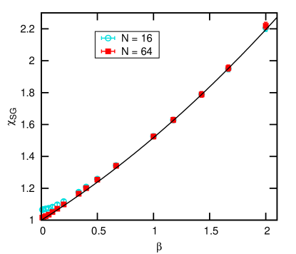
Figure 1: Data for the spin glass susceptibility at small $\beta\,(\equiv 1/T)$ in two dimensions for a concentration $x=1/16$ for $N=16$ and $64$. The curve is a fit to the data for $N=64$. The behavior is clearly linear, not quadratic, at small $\beta$, which is a result of screening. The intercept at $\beta=0$ differs measurably from one for very small sizes only because of the charge neutrality constraint, Eq. (4).

The spin glass susceptibility can be expressed as

$$\chi_{SG} ={1\over N}\sum_{i,j}[C_{ij}^{2}]_{\text{av}}$$

$$=1+{1\over N}\sum_{i\neq j}[C_{ij}^{2}]_{\text{av}}$$ (17)

where $C_{ij}=\langle S_{i}S_{j}\rangle$ and the terms with $i=j$ give unity, which is the result for $T=\infty$. Naively, one can obtain the second term in Eq. (17) at high temperature by expanding the Boltzmann factors in powers of $\beta\,(\equiv 1/T)$, with the result

$$C_{ij}=\beta J_{ij}+O(\beta^{2})\qquad(i\neq j),$$ (18)

but then the sum in the second term in Eq. (17) diverges for the Coulomb potential interaction in Eq. (3). Clearly a resummation of terms is needed to get a finite result. In fact, Ref. Rehn et al. (2015) showed that the interactions are screened up to a length scale $\lambda$ where

$$\lambda\propto\sqrt{T}.$$ (19)

Within certain approximations, the final result of Ref. Rehn et al. (2015) in $d=2$, is

$$C_{ij}\propto\beta K_{0}(r_{ij}/\lambda),$$ (20)

where $K_{0}(x)$ is a modified Bessel functions which decays exponentially to zero at large $x$. This is to be compared with the naive result in Eq. (18) that $C_{ij}=\beta J(\mathbf{r}_{ij})\propto\beta\log(r_{ij})$. Inserting Eq. (20) into Eq. (17) one has, at high-$T$ and in $d=2$,

$$\chi_{SG} =1+\text{const.}\,\lambda^{2}\beta^{2}$$ (21)

$$=1+\text{const.}^{\prime}\,\beta\,.$$ (22)

Hence, because of screening, the leading correction to the infinite-temperature result is of order $\beta$, rather than $\beta^{2}$ which would be the case for short-range interactions. This result is clearly shown by the numerics in Fig. 1.

Because the interactions are screened, we might expect the universality class of the spin glass transition in the disordered Coulomb antiferromagnet to be the same as that of the short-range EA spin glass. Even if this is the case, the fact that the screening length is temperature dependent will give rise to additional, and possibly large, corrections to FSS which could complicate the analysis.

IV.2 Equilibration

To test for equilibration we obtain data for runs of different length in which the number of sweeps doubles for each run, and for all runs we average over the last half of the sweeps. It is easy to see that this can actually be done in a single run by using all the data. We require that the data is independent of run time within small error bars for the last two data points. Figure 2 shows an example for $N=576$ for $d=2$ at the lowest temperature $T=0.032$.

IV.3 Two-dimensions

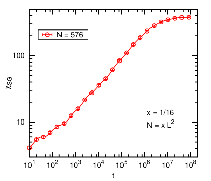
Figure 2: Equilibration plot for $N=576,d=2$ with $x=1/16$ at the lowest temperature of $T=0.032$. The spin glass susceptibility $\chi_{SG}$ is plotted against Monte Carlo sweeps $t$. For each point, averaging is carried out over the last half of the sweeps.

Table 1: Simulation parameters for $d=2$. The concentration is $x=1/16$ where $N=xL^{2}$. For each value of size $N$, $N_{\mathrm{samp}}$ samples were run for $N_{\mathrm{sweep}}$ sweeps with averaging performed over the last half. Parallel tempering Monte Carlo was performed with $N_{T}$ temperatures distributed between $T_{\mathrm{min}}$ and $T_{\mathrm{max}}$.

$N$	$L$	$N_{\mathrm{sweep}}$	$T_{\mathrm{min}}$	$T_{\mathrm{max}}$	$N_{T}$	$N_{\mathrm{samp}}$
64	32	2097152	0.025	1	15	256
144	48	2097152	0.025	0.500	15	1024
256	64	8388608	0.025	0.500	15	767
400	80	16777216	0.025	0.25	15	256
576	96	83886080	0.032	0.500	16	467
784	112	167772160	0.05	0.25	11	96

Now we discuss our results for two-dimensions for which we use a fixed concentration $x=1/16$. The parameters of the simulations are shown Table 1.

For the EA model it is well established that the spin glass transition only occurs at $T=0$ where the correlation length diverges with an exponent $\nu\simeq 3.4$ Bray and Moore (1984); Hartmann and Young (2001); Fernandez et al. (2016) and the exponent $\eta$, which is related to the divergence of the spin glass susceptibility according to Eqs. (14) and (15), is $\eta=0$.

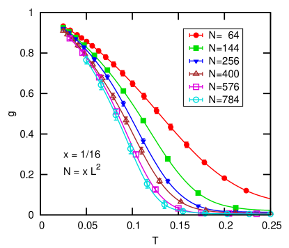
Figure 3: Data for the Binder ratio in $d=2$.

Our data for the Binder ratio $g$ is shown in Fig. 3. There is no sign of any intersections and hence no indication of a finite temperature transition. This is consistent with the EA model in $d=2$. Figure 4 shows a scaling plot according to Eq. (12) assuming $T_{c}=0$. If there is a zero temperature transition the data should collapse, at least for large enough sizes and low enough temperatures. We were not able to collapse the data for all sizes with any choice of the correlation length exponent $\nu$ but the data for the largest sizes collapses fairly well with $\nu\simeq 3.5$ (as shown) consistent with results for the EA model. However, there is a large uncertainty in this estimate; we find that any value for $\nu$ in the range $2.7$ to $4.5$ gives a plausible fit for large sizes.

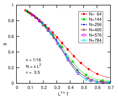
Figure 4: Scaling plot for Binder ratio in $d=2$ according to Eq. (12) with $T_{c}=0$. We are not able to get all the data to collapse for any value of the correlation length exponent $\nu$. However the data for the largest sizes collapses with $\nu\simeq 3.5$ (shown), consistent with the value in the EA model. However, there are big uncertainties in our estimate (see text).

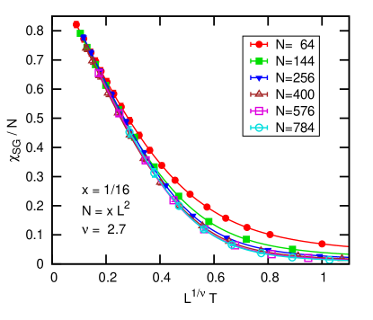
Figure 5: The spin glass susceptibility in $d=2$ scaled according to Eq. (14) with $T_{c}=0$ and $\eta=0$. No value of $\nu$ succeeds in scaling all the data though the largest sizes scale reasonably well with $\nu\simeq 2.7$ (shown), not very different from the value for the EA model of $3.4$. However, there are big uncertainties in our estimate (see text).

In Fig. 5 we show scaled data for $\chi_{SG}$ according to Eq. (14) assuming $T_{c}=0$ and $\eta=0$ (the latter corresponding to a non-degenerate ground state which seems reasonable). As with the data for $g$ in Fig. 4, we can not scale all the data for any value of $\nu$. However, the data for larger sizes scales fairly well with a value of $2.7$ (shown) not very different from the value for the EA model of 3.4. However, there are big uncertainties in our estimate; any value between $2.0$ and $4.0$ gives a plausible collapse for large sizes.

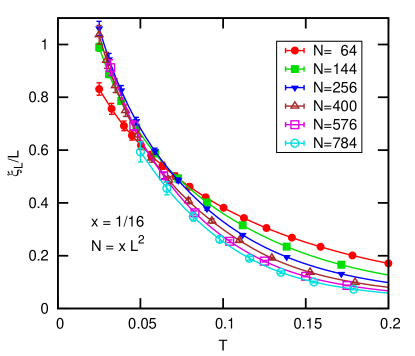
Figure 6: Correlation length divided by system size in $d=2$.

Our attempts to scale the data for $g$ and $\chi_{SG}$ indicate the presence of substantial corrections to FSS for the range of sizes that we can study. This problem is even more severe for the data for $\xi_{L}/L$. Being dimensionless, the data for this quantity should intersect if there is a transition, see Eq. (16). As shown in Fig. 6 there is an intersection involving the smallest size studied, $N=64$, but not for larger sizes. Rather the data for larger sizes seems to merge at low-$T$. If we try to scale the data for $\xi_{L}/L$ we need a large value of $\nu$ to collapse the data for large sizes. Figure 7 shows the result with $\nu=5.0$. These results indicate that the data for $\xi_{L}/L$ is not at large enough sizes to give a clear prediction for the nature of the transition.

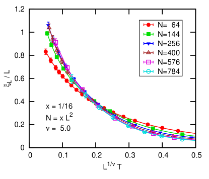
Figure 7: Scaling plot of the correlation length divided by system size in $d=2$ assuming $\nu=5.0$.

IV.4 Three-dimensions

Table 2: Simulation parameters for $d=3$. The concentration is $x=1/64$ where $N=xL^{3}$. For each value of size $N$, $N_{\mathrm{samp}}$ samples were run for $N_{\mathrm{sweep}}$ sweeps with averaging performed over the last half. Parallel tempering Monte Carlo was performed with $N_{T}$ temperatures distributed between $T_{\mathrm{min}}$ and $T_{\mathrm{max}}$.

$N$	$L$	$N_{\mathrm{sweep}}$	$T_{\mathrm{min}}$	$T_{\mathrm{max}}$	$N_{T}$	$N_{\mathrm{samp}}$
64	16	20480	0.0100	0.2000	9	1000
216	24	1310720	0.0100	0.2000	12	400
512	32	41943040	0.0200	0.2150	15	360
1000	40	83886080	0.0215	0.1305	15	568

Next we discuss our results for three-dimensions for which we use a fixed concentration $x=1/64$. The parameters of the simulations are shown Table 2. For the EA model in $d=3$ it is firmly established that there is a spin glass transition at non-zero temperature Hasenbusch et al. (2008); Baity-Jesi et al (2013).

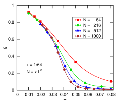
Figure 8: Binder ratio for $d=3$.

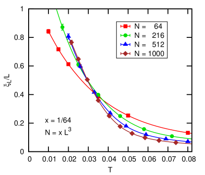
Figure 9: Correlation length divided by system size for $d=3$.

Data for the dimensionless quantities $g$ and $\xi_{L}/L$ are shown in Figs. 8 and 9 respectively. The results for $g$ seem to merge at low-$T$ but do not obviously cross. It should be mentioned that even for the EA model the splaying out of the data for $g$ below $T_{c}$ is only a small effect, see for example Ref. Kawashima and Young (1996), but is, nonetheless, observable with good data on large sizes.

For small sizes the data for $\xi_{L}/L$ shows a large splaying out, but the data for large sizes seems only to merge. Splaying out for the smallest size was also observed in $d=2$, see Fig. 6, and was interpreted as a FSS correction since it disappears for larger sizes. The same is presumably true here; we should give most weight to the data for larger sizes. But the larger size data in Fig. 9 looks very marginal, possibly suggesting that $d=3$ is the lower critical dimension, $d_{l}$. This is different from the EA model where $d_{l}$ is approximately, or possibly exactly Boettcher (2005), equal to $2.5$.

V Conclusions

We have studied spin glass behavior in the random Coulomb Ising antiferromagnet in two and three dimensions by Monte Carlo simulations, with results analyzed by FSS. Since the interactions are screened, and so are effectively short-ranged, a natural hypothesis is that the critical behavior is the same as that of the short-range Ising EA model. For the latter, a transition occurs at $T=0$ in $d=2$ but at a non-zero temperature in $d=3$. Our results indicate a zero temperature transition in $d=2$, with a correlation length exponent compatible with that found for the EA model, though with big error bars. However, in $d=3$, we do not find unambiguous evidence for a non-zero temperature transition temperature. Rather the data for larger sizes seems to be “marginal”. This could indicate that the system sizes are simply not large enough to see the asymptotic critical behavior, or it could be that our model is not in the same universality class as that of the short-range Ising EA model, but rather has a different lower critical dimension, $d_{l}=3$ rather than $d_{l}=2.5$ for the EA model. If this is the case, the nature of the physics causing the difference in universal behavior is unclear to us.

There are clearly large corrections to FSS for this problem, the data for the correlation length in Figs. 6 and 9 providing striking examples. As well as corrections to scaling that occur for the short-range EA model, here we have an additional contribution because the screening length is temperature-dependent. In fact, according to Ref. Rehn et al. (2015) the screening length is singular for $T\to 0$, see Eq. (19). If this result holds down to $T=0$ it could possibly change the critical behavior in $d=2$, where the transition is also at zero temperature, rather than simply giving a correction to scaling. In $d=3$, the transition is at finite-$T$ for the EA model, so we expect only a correction to scaling from the $T$-dependence of $\lambda$.

We close on a historical note. The question of whether or not there is a finite temperature transition in the $d=3$ Ising EA spin glass was controversial for many years. It was only later, when better FSS methods were developed and computers became more powerful, that the question was definitely answered in the affirmative. Perhaps, therefore, it is not surprising that this early effort on a Coulomb spin glass does not leave to a definite conclusion, given the extra difficulties of long-range interactions and larger corrections to scaling.