Deterministic strong-field quantum control

Abstract

Strong-field quantum-state control is investigated, taking advantage of the full—amplitude and phase—characterization of the interaction between matter and intense ultrashort pulses via transient-absorption spectroscopy. A sequence of intense delayed pulses is used, whose parameters are tailored to steer the system into a desired quantum state. We show how to experimentally enable this optimization by retrieving all quantum features of the light-matter interaction from observable spectra. This provides a full characterization of the action of strong fields on the atomic system, including the dependence upon possibly unknown pulse properties and atomic structures. Precision and robustness of the scheme are tested, in the presence of surrounding atomic levels influencing the system’s dynamics.

The advent of laser light and femtosecond pulse-shaping technology have revolutionized our access to the quantum properties of matter Brif et al. (2010); Tannor (2007); Peirce et al. (1988), with coherent-control methods exploiting interference in order to steer a system into a given state with light Brumer and Shapiro (1992); Judson and Rabitz (1992); Meshulach and Silberberg (1998); Weinacht et al. (1999); Brixner et al. (2001). Measurement-driven techniques such as adaptive feedback control are extensively used, especially when little understanding of the light-matter interaction is available owing to inaccurately known atomic or molecular structures, nonideal experimental conditions, or because of the use of strong, insufficiently characterized laser fields. Femtosecond pulses are thus utilized to simultaneously control and interrogate the atomic system, with their shape being iteratively optimized based on the received experimental response Judson and Rabitz (1992). However, the associated atomic dynamics remain concealed in the optimal pulse, often preventing insight into the underlying physical mechanism. Only recently techniques were investigated to access the complex reaction pathways followed by an optimally controlled system Daniel et al. (2003); Rey-de-Castro et al. (2013) and in the strong-field regime, where perturbative approaches fail and the atomic level structure is dressed by the time-dependent field, a limited number of effective pulse-shaping strategies has been identified Dudovich et al. (2005); Clow et al. (2008); Bayer et al. (2009); Bruner et al. (2010).

Major advances in x-ray free-electron lasers (FELs) are now enabling quantum control also at short wavelengths Pellegrini et al. (2016). Coherent transform-limited x-ray pulses are produced via seeding methods at FELs Amann et al. (2012); Allaria et al. (2012), opening the field of x-ray quantum optics Adams et al. (2013). Despite recent advances Gauthier et al. (2015); Prince et al. (2016), however, experimental challenges still need be faced. Complex spectral-shaping methods are not yet available at short wavelengths, in particular for hard x rays, and control schemes, e.g., to manipulate several excited states lying within the x-ray pulse bandwidth, should preferably rely on optimal pulse sequences. Methods to measure pulse temporal profiles are significantly hindered at x-ray frequencies by the absence of suitable nonlinear crystals. Therefore, measurement-driven strategies directly accessing the atomic response to intense, insufficiently characterized pulses should be preferred to methods based on theoretical assumptions of the pulse shape. At the same time, the reduced flexibility at recently established x-ray FELs renders adaptive feedback still very challenging for current experiments.

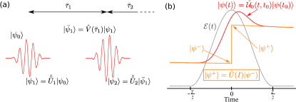
Figure 1: (Color online). (a) Quantum-control scheme based on an optimal sequence of experimentally characterized pulses. (b) Interaction of a quantum system (red, continuous line) with an ultrashort pulse (gray, dashed line), effectively modeled as an instantaneous effect (orange, continuous line).

In order to determine an effective route to x-ray quantum control despite present limitations, in this Letter we put forward a scheme to experimentally characterize—in amplitude and phase—the atomic interaction with intense ultrashort pulses, and use this information to deterministically guide the system into a desired state with an optimal pulse sequence [Fig. 1(a)]. Thereby, one keeps the advantages of a measurement-driven strategy. In stark contrast to adaptive feedback, however, where optimal pulse shapes are iteratively determined via a trial-and-error procedure, our scheme allows access and visualization of the building blocks constituting the optimal strong-field control strategy, providing an advantageous means to unravel the dynamical pathways followed by the system. Furthermore, for experimental conditions in which feedback may not be advisable due to, e.g., restricted beam time, our scheme represents a cost-effective strategy to prepare a given system in different states: adaptive feedback requires a new sequence of iterations for every desired state, whereas deterministic strong-field control could be performed numerically relying on a set of elementary steps characterized experimentally. Motivated by recent results Liu et al. (2015), the scheme is applied here to control optical transitions in Rb atoms, but it could be straightforwardly implemented at x-ray energies with, e.g., highly charged ions, among the best candidates for future x-ray quantum-optics applications Adams et al. (2013).

Interaction operators. The key quantity we will use to characterize the atomic response to intense ultrashort pulses is the interaction operator $\hat{U}(I)$, whose action is represented in Fig. 1(b). We assume a pulse of the form $\bm{\mathcal{E}}(t)=\mathcal{E}_{0}\,f\left(t\right)\,\cos\left(\omega_{\mathrm{L}}t\right)\hat{\bm{e}}_{z}$, linearly polarized along the $\hat{\bm{e}}_{z}$ unit vector, with laser frequency $\omega_{\mathrm{L}}=1.59\,\mathrm{eV}$ and peak field strength $\mathcal{E}_{0}=\sqrt{8\pi\alpha I}$, where $I$ is the pulse peak intensity and $\alpha$ the fine-structure constant Diels and Rudolph (2006). The envelope function $f(t)$ is nonvanishing in the interval $[-T/2,\,T/2]$, with pulse duration $T$. Atomic units are used unless stated otherwise. In the absence of external fields, the known free evolution of the system under the action of the atomic structure Hamiltonian $\hat{H}_{0}$ is given by $\hat{V}(t)=\mathrm{e}^{-\mathrm{i}\hat{H}_{0}t}$. In the interval $[-T/2,\,T/2]$, however, the dynamics of the system $|\psi(t)\rangle=\hat{\mathcal{U}}_{0}(t,t_{0})|\psi(t_{0})\rangle$, depicted in Fig. 1(b), require the solution of the Schrödinger equation in the presence of the external pulse $\bm{\mathcal{E}}(t)$. In order to operatively describe this strong-field interaction, we introduce the effective initial and final states $|\psi^{\mp}\rangle=\mathrm{e}^{\mathrm{i}\hat{H}_{0}(\mp T/2)}|\psi(\mp T/2)\rangle$, represented in Fig. 1(b). The unique, intensity-dependent operator $\hat{U}(I)=\mathrm{e}^{-\mathrm{i}\hat{H}_{0}(-T/2)}\hat{\mathcal{U}}_{0}\left(T/2,-T/2\right)\mathrm{e}^{\mathrm{i}\hat{H}_{0}(T/2)}$, connecting $|\psi^{+}\rangle$ with $|\psi^{-}\rangle$,

$$|\psi^{+}\rangle=\hat{U}(I)|\psi^{-}\rangle,$$ (1)

is used to effectively describe the action of an ultrashort pulse in terms of a $\delta$-like interaction Santra et al. (2011); Blättermann et al. (2014).

Endowed with an efficient way to quantify the action of strong ultrashort pulses, we can summarize our deterministic quantum-control scheme as follows. To prepare a system in a desired state $|\psi_{\mathrm{d}}\rangle$, we use the sequence of $N_{\mathrm{p}}$ pulses shown in Fig. 1(a), separated by delays $\bar{\tau}_{m}$ and leading the system to the state

$$|\psi_{N_{\mathrm{p}}}\rangle=\hat{\tilde{U}}_{N_{\mathrm{p}}}\ldots\hat{V}(\bar{\tau}_{m})\hat{\tilde{U}}_{m}\ldots\hat{V}(\bar{\tau}_{1})\hat{\tilde{U}}_{1}|\psi_{\mathrm{0}}\rangle.$$ (2)

Here, the action of the $m$th pulse is described by $\hat{\tilde{U}}_{m}=\hat{\varPhi}^{\dagger}(\phi_{m})\,\hat{U}(I_{m})\,\hat{\varPhi}(\phi_{m})$, with intensity $I_{m}$ and where $\hat{\varPhi}(\phi_{m})$ accounts for a carrier-envelope phase (CEP) $\phi_{m}$. In adaptive feedback, a series of experiments is performed for every desired state $|\psi_{\mathrm{d}}\rangle$, iteratively searching for the optimal combinations of pulse delays, CEPs, and intensities. Little knowledge is thereby achieved about the possible pathways the system could follow and the rules determining the optimal pulse sequence. In contrast, in deterministic strong-field control, experiments are first run to fully characterize the interaction operators $\hat{U}(I)$, providing a complete experimental mapping of the available control options and facilitating manipulation and interpretation of the chosen control strategy. Although interaction operators could be calculated from theory, our deterministic scheme allows one to effectively tackle those cases where reliable predictions are not possible via methods based exclusively on theory, due to missing knowledge of the atomic structures, pulse shapes, or the strong-field interaction.

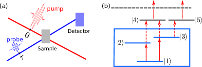
Figure 2: (Color online). (a) Transient-absorption-spectroscopy setup used to experimentally reconstruct strong-field interaction operators. (b) Level scheme used to model Rb atoms, aiming at the control of the $V$-type three-level scheme in the box.

Reconstruction of the strong-field interaction operators. To exploit the advantages of a measurement-driven strategy without employing adaptive feedback, we utilize transient-absorption spectroscopy (TAS) to reconstruct $\hat{U}(I)$ in amplitude and phase, and use these extracted matrices for quantum-state control. TAS has been receiving increasing interest for studies of ultrafast dynamics Mathies et al. (1988); Pollard and Mathies (1992); Loh et al. (2007); Wang et al. (2010); Goulielmakis et al. (2010); Holler et al. (2011); Ott et al. (2013); Wu et al. (2016); Meyer et al. (2015). In a pump-probe setup, depicted in Fig. 2(a), the absorption spectrum $\mathcal{S}(\omega,\tau)$ of a transmitted weak probe pulse is observed for varying time delays $\tau$, revealing the dynamics initiated by the intense pump pulse Fano and Cooper (1968). At the same time, recent experiments have employed a probe-pump scheme ($\tau<0$), with the probe pulse generating a coherent superposition of quantum states which is subsequently nonlinearly excited by the strong pulse Wang et al. (2010); Chen et al. (2012); Beck et al. (2014); Kaldun et al. (2014). In this case, absorption spectral line shapes contain valuable information to quantify the strong-field dynamics induced by the pump pulse, albeit requiring schemes to extract information from complex time-dependent spectra. Characterizing strong-field interactions to reconstruct $\hat{U}(I)$ with TAS can be straightforwardly implemented experimentally, since the same intense pulse is used with varying time delays. This minimizes the number of experiments where pulse parameters need be precisely modified, in contrast to adaptive feedback, where pulse intensities, phases and delays are simultaneously and controllably varied at every iteration to converge to the desired state.

We apply our scheme to Rb atoms Netz et al. (2002); Liu et al. (2015). Specifically, we aim at controlling the $V$-type three-level system formed by the ground state $5s\,^{2}S_{1/2}\equiv|1\rangle$ and fine-structure-split excited states $5p\,^{2}P_{1/2}\equiv|2\rangle$ and $5p\,^{2}P_{3/2}\equiv|3\rangle$, with magnetic quantum numbers $M=\pm 1/2$ and transition energies $\omega_{21}=1.56\,\mathrm{eV}$ and $\omega_{31}=1.59\,\mathrm{eV}$. The electric-dipole-($E1$-)allowed transitions $|1\rangle\rightarrow|k\rangle$, $k\in\{2,\,3\}$ [box in Fig. 2(b)] feature $\Delta M=0$ and dipole-moment matrix elements $\bm{D}_{1k}=D_{1k}\hat{\bm{e}}_{z}$ Theodosiou (1984). The decay of the system is accounted for in the atomic structure Hamiltonian $\hat{H}_{0}=\sum_{i}{(\omega_{i}-\mathrm{i}\gamma_{i}/2)|i\rangle\langle i|}$, while the interaction with femtosecond pump and probe pulses, respectively centered on $t=0$ and $t=\tau$, is included via the $E1$ interaction Hamiltonian in the rotating-wave approximation Scully and Zubairy (1997). $\gamma_{k}$ are set to $1/(1500\,\mathrm{fs})$ to model experimental finite linewidths due to, e.g., Doppler and collision-induced broadening. The much smaller spontaneous-decay rates, of $\sim\mathrm{ns}^{-1}$, can be neglected for the femtosecond time scales of interest. A Schrödinger formalism is used to describe the state of the system, whereas a more thorough treatment based on density matrices is presented in the Supplemental Information.

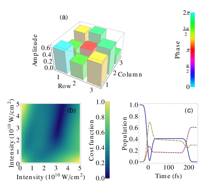
Figure 3: (Color online). (a) Reconstructed SFI operator $\hat{U}^{\mathrm{R}}(I)$ for $I=3.3\times 10^{10}\,\mathrm{W/cm^{2}}$, with bar heights (colors) exhibiting matrix-element amplitudes (phases). [(b)-(c)] Two-pulse scheme implemented for $I_{1}=3.3\times 10^{10}\,\mathrm{W/cm^{2}}$, $I_{2}=3.6\times 10^{10}\,\mathrm{W/cm^{2}}$, $\bar{\tau}=198\,\mathrm{fs}$, and $\bar{\phi}=1.88\,\mathrm{rad}$, with (b) a section of the control landscape as a function of $I_{1}$ and $I_{2}$, for fixed $\bar{\tau}$ and $\bar{\phi}$ and (c) the corresponding evolution of the populations of state $|1\rangle$ (blue, continuous), $|2\rangle$ (purple, dashed), and $|3\rangle$ (yellow, dotdashed), with a reached final state $|\psi_{\mathrm{r}}\rangle=\sum_{i=1}^{3}c_{\mathrm{r},i}|i\rangle$ featuring $|c_{\mathrm{r},2}|^{2}/|c_{\mathrm{r},3}|^{2}=2.07$ and $c_{\mathrm{r},1}=0.00$.

For low densities, where propagation effects can be neglected and the pulses can be assumed to homogeneously control the sample, the time-delay-dependent spectra result from the system’s single-particle dipole response,

$$\mathcal{S}(\omega,\tau)\propto-\omega\mathop{}\!\mathbf{Im}\left[\hat{\bm{e}}_{z}\cdot\int_{-\infty}^{\infty}\left\langle\hat{\bm{D}}^{-}(t,\tau)\right\rangle\,\mathrm{e}^{-\mathrm{i}\omega(t-\tau)}\mathop{}\!\mathrm{d}t\right],$$ (3)

where $\langle\hat{\bm{D}}^{-}(t,\tau)\rangle=\left\langle\psi(t,\tau)\right|\hat{\bm{D}}^{-}\left|\psi(t,\tau)\right\rangle$ is the expectation value of the dipole-moment operator $\hat{\bm{D}}^{-}=\sum_{i>j}\bm{D}_{ij}|i\rangle\langle j|$, and $|\psi(t,\tau)\rangle$ describes the time evolution of the system as a function of time delay. We use Eq. (3) to numerically simulate experimental spectra $\mathcal{S}_{\mathrm{exp}}(\omega,\tau)$ for pump pulses of intensities varying between $0.1\times 10^{10}\,\mathrm{W/cm^{2}}$ and $5\times 10^{10}\,\mathrm{W/cm^{2}}$ and for the noncollinear geometry of Fig. 2(a) Liu et al. (2015). This is based on the full solution of the Schrödinger equation for a three-level system interacting with delayed pump and probe pulses. At the same time, Eq. (3) is also used to derive a fitting model for transient-absorption spectra and, thereby, enable the extraction of strong-field interaction (SFI) operators. For this purpose, we take advantage of the same instantaneous-interaction model introduced in Eq. (1) and formally describe the system’s dynamics in a pump-probe experiment in terms of the operators $\hat{U}_{\mathrm{pr}}$ and $\hat{U}_{\mathrm{pu}}(I)$. For weak probe pulses, first-order perturbation theory is used to model $\hat{U}_{\mathrm{pr}}$, whereas the matrix elements $U_{\mathrm{pu},ij}$ of the intensity-dependent pump-pulse operator $\hat{U}_{\mathrm{pu}}(I)$ are unknown fitting parameters. For $\tau<0$, the effective evolution of the time-delay-dependent state $\left|\psi_{\mathrm{fit}}(t,\tau)\right\rangle$ from the initial state $|\psi_{0}\rangle=|1\rangle$ can be modeled as

$$|\psi_{\mathrm{fit}}(t,\tau)\rangle=\left\{\begin{aligned} &|\psi_{0}\rangle,&\text{if $t<\tau$},\\ &\hat{V}(t-\tau)\hat{U}_{\mathrm{pr}}|\psi_{0}\rangle,&\text{if $\tau<t<0$},\\ &\hat{V}(t)\hat{U}_{\mathrm{pu}}(I)\,\hat{V}(-\tau)\,\hat{U}_{\mathrm{pr}}|\psi_{0}\rangle,&\text{if $t>0$},\end{aligned}\right.$$ (4)

with analogous formulas for $\tau>0$. Inserting this in Eq. (3), an analytical fitting model $\mathcal{S}_{\mathrm{fit}}(\omega,\tau,U_{\mathrm{pu},ij})$ can be derived (see details in the Supplemental Information) and used to fit the experimental spectra $\mathcal{S}_{\mathrm{exp}}(\omega,\tau)$ and reconstruct the SFI operators $\hat{U}^{\mathrm{R}}(I)$ in amplitude and phase:

$$\left.\begin{aligned} \mathcal{S}_{\mathrm{exp}}(\omega,\tau)\\ \mathcal{S}_{\mathrm{fit}}(\omega,\tau,U_{\mathrm{pu},ij})\end{aligned}\right\}\underset{\text{fitting}}{\longrightarrow}\text{Reconstructed operator $\hat{U}^{\mathrm{R}}$}.$$ (5)

The effectiveness of the method is exemplified in Fig. 3(a), where we display the extracted SFI matrix $\hat{U}^{\mathrm{R}}(I)$ for a pump intensity of $I=3.3\times 10^{10}\,\mathrm{W/cm^{2}}$. The same reconstruction scheme could be implemented in an experiment, enabling access to strong-field light-matter interactions without requiring knowledge of pump-pulse intensities or the system’s dynamics.

Quantum control guided by experimentally characterized pulses. Once SFI operators are reconstructed as a function of pulse intensities, these are employed to implement our deterministic control method from Eq. (2). In the following, we focus on a two-pulse scheme, and use reconstructed SFI operators to optimize time separation $\bar{\tau}$, intensities $I_{m}$, and CEPs $\phi_{m}$, $m\in\{1,\,2\}$, to control the populations of the final state $|\psi_{2}\rangle$. This yields a predicted final state

$$|\psi_{\mathrm{p}}\rangle={\textstyle\sum_{i=1}^{3}}c_{\mathrm{p},i}|i\rangle=\hat{U}^{\mathrm{R}}(I_{2})\,\hat{\varPhi}(\bar{\phi})\,\hat{W}(\bar{\tau})\,\hat{U}^{\mathrm{R}}(I_{1})\,|1\rangle,$$ (6)

where we neglect phase terms not influencing the final populations, and introduce the total phase $\bar{\phi}=\phi_{2}-\phi_{1}-\omega_{\mathrm{L}}\bar{\tau}$, the CEP operator $\hat{\varPhi}(\phi)=\mathrm{diag}(1,\,\mathrm{e}^{\mathrm{i}\phi},\,\mathrm{e}^{\mathrm{i}\phi})$, and the slowly oscillating operator $\hat{W}(\bar{\tau})=\mathrm{diag}\left(1,\,\mathrm{e}^{-[\gamma_{2}/2+\mathrm{i}(\omega_{21}-\omega_{\mathrm{L}})]\bar{\tau}},\,\mathrm{e}^{-[\gamma_{3}/2+\mathrm{i}(\omega_{31}-\omega_{\mathrm{L}})]\bar{\tau}}\right)$.

In order to show how coherently controlled dynamics can be interpreted in terms of experimentally reconstructed SFI operators, in Fig. 3 we present results for a sequence of two strong pulses aiming at the desired state $|\psi_{\mathrm{d}}\rangle=\sum_{i=1}^{3}c_{\mathrm{d},i}|i\rangle$, of amplitudes $(c_{\mathrm{d},1},\,c_{\mathrm{d},2},\,c_{\mathrm{d},3})=A\mathrm{e}^{\mathrm{i}\gamma}\,(0,\,\sqrt{2/3},\,\mathrm{e}^{\mathrm{i}\delta}\sqrt{1/3})$, such that the ground state is completely depopulated, while the excited state $|2\rangle$ is twice as much populated as $|3\rangle$, despite a less favorable coupling to the ground state. The total final population $A^{2}$ and the phases $\gamma$ and $\delta$ are free parameters. Optimal pulse properties are determined via minimization of the cost function Brif et al. (2010)

$$g(I_{1},I_{2},\bar{\tau},\bar{\phi})=\sqrt{{\textstyle\sum_{i=1}^{3}}\bigl{|}|{c}_{\mathrm{d},i}|^{2}-|{c}_{\mathrm{p},i}|^{2}\bigr{|}^{2}},$$ (7)

calculated for a discrete set of parameters and ensuring that $|\langle\psi_{\mathrm{d}}|\psi_{\mathrm{d}}\rangle|^{2}=|\langle\psi_{\mathrm{p}}|\psi_{\mathrm{p}}\rangle|^{2}=A^{2}$. A section of the control landscape Brif et al. (2010), associated with global minima of the cost function $g$, is displayed in Fig. 3(b), confirming that it is a smooth function of its parameters, and small uncertainties in the pulse intensities do not lead to final states significantly differing from those expected. Figure 3(c) shows the resulting dynamics of the system, when excited with the sequence of pulses determined via minimization of $g$, exhibiting very good agreement with the desired final state. The displayed dynamics could be directly inferred from the reconstructed SFI operators. The state reached after the first intense pulse in Fig. 3(c) is completely encoded in the matrix elements plotted in Fig. 3(a), such that deterministic strong-field control provides an experiment-based visualization of the building blocks exploited by optimal control to reach a desired state. Rabi oscillations induced by strong ultrashort pulses are apparent in Fig. 3(c), but knowledge of their explicit time dependence is not necessary to control the reached final state. Although we focus on the control of final populations, this nevertheless requires phase knowledge of $\hat{U}^{\mathrm{R}}(I)$, such that $\hat{\varPhi}(\bar{\phi})$ and $\hat{V}(\bar{\tau})$ can ensure the necessary relative phase upon arrival of the second pulse Tannor (2007).

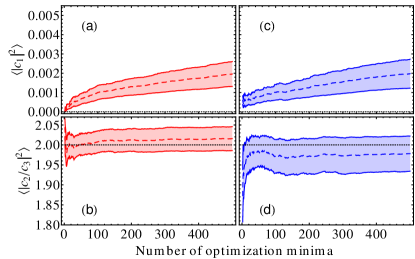
Figure 4: (Color online). [(a),(c)] Reached ground-state population and [(b),(d)] ratio of the populations of the two excited states $|2\rangle$ and $|3\rangle$, averaged over the $N$ best sets of optimization pulse parameters $\{I_{1},\,I_{2},\,\bar{\tau},\,\bar{\phi}\}$, as a function of $N$. Mean values are displayed as dashed lines, the surrounding regions (bounded by continuous lines) have an amplitude given by the corresponding standard deviation. Desired final population and ratios are exhibited by black, dotted lines. Reached final populations and ratios are calculated for [(a),(b)] a three-level-only system and [(c),(d)] a five-level system. The best optimization parameters are obtained via minimization of the cost function (7), calculated with SFI operators $\hat{U}^{\mathrm{R}}(I)$ reconstructed from transient-absorption spectra numerically simulated for [(a),(b)] a three-level and [(c),(d)] a five-level model.

To verify the precision of the scheme, in Fig. 4(a) and 4(b) we display final populations reached by the three-level system when using sequences of pulses determined through the minimization of Eq. (7). The extracted SFI operators have an intrinsic uncertainty, and we therefore display results averaged among the first $N$ best sets of optimization parameters—with standard deviation—, as a function of $N$. Very good control performances are exhibited: complete depopulation of the ground state is reached [Fig. 4(a)], and the mean value of the ratio $|c_{2}/c_{3}|^{2}$ is equal to 2 for the first best sets of optimization parameters, with relative uncertainty of $\sim 3\%$ [Fig. 4(b)].

Finally, we test our scheme in a realistic scenario, characterized by the presence of incomplete modeling or perturbations. To derive $\mathcal{S}_{\mathrm{fit}}(\omega,\tau,U_{\mathrm{pu},ij})$ from Eq. (3), basic knowledge of the atomic transitions responsible for the absorption lines appearing in the spectrum is necessary. A robust control scheme should enable the manipulation of the states of interest also when additional, moderately contributing levels are present, which may not be known or experimentally discernible. As an example, we employ the fitting model $\mathcal{S}_{\mathrm{fit}}(\omega,\tau,U_{\mathrm{pu},ij})$ to extract $3\times 3$ SFI operators $\hat{U}^{\mathrm{R}}$ from transient-absorption spectra in Rb atoms, stemming from the complete numerical simulation of the dynamics of the five-level system displayed in Fig. 2(b). The $E1$-allowed transitions $|2\rangle\rightarrow|4\rangle$, $|3\rangle\rightarrow|4\rangle$, and $|3\rangle\rightarrow|5\rangle$, with $\Delta M=0$, with transition energies $\omega_{42}=1.63\,\mathrm{eV}$ and $\omega_{53}=1.60\,\mathrm{eV}$, are resonantly excited by the optical pulses, albeit more weakly than the $|1\rangle\rightarrow|k\rangle$ transitions, $k\in\{2,\,3\}$, owing to smaller dipole-moment matrix elements $\bm{D}_{kl}=D_{kl}\hat{\bm{e}}_{z}$, $l\in\{4,\,5\}$ Bayram et al. (2000); Safronova et al. (2004). To ensure that this resonant coupling contributes moderately, we assume large linewidths $\gamma_{4}$ and $\gamma_{5}$, here set equal to $1/(100\,\mathrm{fs})$ , such that only the two lines associated with the $|1\rangle\rightarrow|k\rangle$ transitions can be clearly distinguished in the absorption spectra. Photoionization in the presence of an optical pulse is also accounted for LAN . SFI operators $\hat{U}^{\mathrm{R}}(I)$ are extracted from these numerically calculated spectra, and used to control the three-level system in the box of Fig. 2(b) via minimization of the cost function $g$. The very good performances displayed in Figs. 4(c) and 4(d) confirm that the method is robust and only marginally influenced by additional levels not accounted for explicitly in $\mathcal{S}_{\mathrm{fit}}(\omega,\tau,U_{\mathrm{pu},ij})$. Furthermore, in contrast to methods based exclusively on theory, maximal information on the strong-field interaction is extracted from the experimental spectra, including the background effect of unknown additional levels on the SFI operators $\hat{U}^{\mathrm{R}}(I)$ of interest.

In conclusion, we have designed an optimized sequence for quantum-state control based on intensity-dependent operators extractable from observable transient-absorption spectra. Schemes consisting of a higher number of pulses are possible to further enhance the control precision or to achieve additional control goals simultaneously. The method was mainly discussed for a three-level scheme modeling Rb atoms, but this could be straightforwardly generalized to higher numbers of states. Our results are expected to trigger the development of related techniques for interaction-operator reconstruction of more complex systems such as molecules, for which strong-field absorption-line-shape control was recently demonstrated Meyer et al. (2015). The advances in coherent x-ray sources open up interesting prospects especially for the application of our method at short wavelengths. Quantifying the effect of strong broadband pulses from experimentally accessible spectra would then enable quantum control based on designed sequences of the available, ultrashort x-ray pulses, with added benefits such as site specificity near core transitions.