Generalized Optimal Liquidation Problems Across Multiple Trading Venues

Abstract

In this paper, we generalize the Almgren-Chriss’s market impact model to a more realistic and flexible framework and employ it to derive and analyze some aspects of optimal liquidation problem in a security market. We illustrate how a trader’s liquidation strategy alters when multiple venues and extra information are brought into the security market and detected by the trader. This study gives some new insights into the relationship between liquidation strategy and market liquidity, and provides a multi-scale approach to the optimal liquidation problem with randomly varying volatility.

Keywords: Dynamic Programming (DP); Hamilton-Jacobi-Bellman (HJB) Equation; Limit Order (LO); Market Order (MO); Multi-scale Stochastic Volatility Model; Quadratic Variation.

1 Introduction

The optimal liquidation problem of large trades has been studied extensively in the micro-structure literature. Two major sources of risk faced by large traders are: (i) inventory risk arising from uncertainty in asset value; and (ii) transaction costs arising from market friction. In a frictionless and competitive market, an asset can be traded with any amount at any rate without affecting the market price of the asset. The optimal liquidation problem then becomes an optimal stopping problem. In an incomplete market, the optimal liquidation problem involves delicate market-micro-structural issues. The impacts of transaction costs on optimal liquidation and optimal portfolio selection have been studied via various mechanisms [1, 2, 3, 4, 8, 19].

In this paper, we adopt a simple, but practical market impact model to study some aspects of the optimal liquidation problem. The model is phenomenological and not directly based on the fine details of micro-structure though it may primarily be related to some literature on market micro-structure. Following Almgren and Chriss [1], we decompose the price impact into temporary price impact and permanent price impact. Temporary impact refers to temporary imbalance in supply/demand caused by trading. It disappears immediately when trading activities cease. Permanent impact means changes in the “equilibrium” price due to trading, which lasts at least for the whole process of liquidation.

We generalize the work of Almgren and Chriss [1] to a more realistic and flexible framework in which multiple venues are available for the trader to submit his/her trades. We mainly consider short-term liquidation problem for a large trader who experiences temporary and permanent market impact. Two broad classes of problems are addressed in this paper which we believe are representative. The first one is the case with constant volatility. This assumption considerably simplifies the problem and allows us to exhibit the essential features of liquidation across multiple venues without losing ourselves in complexities. The second one is the case when volatility varies randomly throughout the trading horizon. In this case, we present a “pure” stochastic volatility approach, in which the volatility is modeled as an Itô process driven by a Brownian motion that has a component independent of the Brownian motion driving the asset price. In comparison with Almgren’s work in [4], we mainly focus on a special class of volatility model, the time-scale volatility model proposed in [9, 10]:

$$d\nu_{t}=\epsilon(m-\nu_{t})dt+\xi\sqrt{\epsilon}dW_{t},$$

and work in the regime $\epsilon\ll 1$. The separation of time-scales provides an efficient way to identify and track the effect of stochastic volatility, which is desirable from the practical perspective.

We also generalize our basic model to include the usage of limit orders. Different from market orders, limit orders are designed to give investors more flexibility over the buying and selling prices of their trades. The most unfavorable feature of limit orders might be the execution risk, i.e., a successful execution is not guaranteed. Cartea and Jaimungal [7] have constructed optimal strategies for this problem under temporary-impact-only assumption. In their model, and also in ours, investors are allowed to trade both via limit sell orders, whose execution are uncertain, and via market sell orders, whose execution are immediate but costly. Limit orders in their model are allowed to be continuously submitted. Market orders, however, are only for one unit, and are executed at a sequence of increasing stopping times. This model works well for small- and mid-size orders. However, when it comes to large orders, execution cannot be guaranteed. Furthermore, the optimal stopping time setting makes the problem difficult to be solved. To ensure execution and track the trace of liquidating strategy, we model the market orders strategy as a continuous control problem. When other market participants’ buy market orders arrive, limit sell orders will be used instead to take advantage of the price gap.

As mentioned in Rudloff et al. [18], a major reason for developing dynamic models instead of static ones is the fact that one can incorporate the flexibility of dynamic decisions to improve our objective function. Time-inconsistent criteria are generally not favorable to introduce in the study, since the associated policies are sub-optimal. The mean-variance criterion is popular for taking both return and risk into account. However, the mean-variance criterion may induce a potential problem of time-inconsistency, i.e., planned and implemented policies are different, and make the problem complicated. Hence, to take both return and risk into account, instead of adopting the mean-variance criterion, we are most interested in the mean-quadratic optimal agency liquidation strategies, as they are proved to be time-consistent in [11, 12].

In the following, we outline the major contributions of this paper. First, we obtain closed-form solutions for optimal liquidation strategy under the constant volatility approach for any level of risk aversion. This leads to an efficient frontier of optimal strategies. Each point on this frontier represents a strategy with the minimal level of cost for its level of risk-aversion. In addition, we also show that in the presence of multiple venues, institutional traders might hide their liquidating purposes and reduce the permanent market impacts through splitting their orders across multiple venues. When more trading venues spring up in financial market, the liquidity of the market enhances. This provides good suppliers of liquidity to the traders, and that the trader with more choices of venues to submit his/her trades may be willing to close his/her position as soon as possible. Second, we present a framework for the liquidation problem that is general enough to include the effect of stochastic volatility. Moreover, it is tractable and the parameters can be estimated efficiently on large datasets that are increasing available. Third, we study the effect of incorporating limit orders so as to detect market information. In general, for a pure liquidation problem, people do not include the usage of limit orders. But in our study of including limit orders, we find that, realizing the information carried by other market participants, traders will slow down their liquidating speed so as to get profit from market momentum.

The remainder of this paper is organized as follows. Section 2 devotes to model building for the execution problem in the presence of multiple trading venues. The Profit & Loss (P&L) of trading and a mean-quadratic-variation criterion are proposed and discussed in this section. The solutions and numerical results for the constant volatility approximation are presented in Section 3. Extension of the results to the stochastic volatility approximation are then discussed in Section 4. An extension of our model to the incorporation of limit orders is studied in Section 5. The final section summarizes the results.

2 Problem Setup

In this section, we first present our liquidation problem in the presence of multiple trading venues based on the principle of no arbitrage. We then discuss the optimal liquidating strategies.

2.1 The Trader’s Liquidation Problem

We consider an institutional trader. Beginning at time $t=0$, he/she has a liquidation target of $Q$ shares, which must be completed by time $t=T$. The number of shares remaining to liquidate at time $t$ is the trajectory $X_{t}$, with $X_{0}=Q$ and $X_{T}=0$. Suppose there are $N$ distinct venues for the trader to submit his/her trades. The rate of liquidating in Venue $n$ ($n=1,2,\ldots,N$) is $\theta^{(n)}_{t}$. Thus,

$$\theta^{(1)}_{t}+\cdots+\theta^{(N)}_{t}=-\frac{dX_{t}}{dt}.$$

For a liquidation program, $Q>0$, we expect $X_{t}\geq 0$ is decreasing and $\theta^{(n)}_{t}\geq 0$ (a buy program may be modeled similarly). Here, $\theta^{(n)}_{t}$ ($n=1,2,\ldots,N$), are the choice variables or decision variables of the trader at time $t$ based on the observed information available at time $t$. In general, the trajectory $X_{t}$ depends on the price movements and market conditions that are discovered during trading, so it is a stochastic process.

Consider a probability space $(\Omega,\mathcal{F},\mathcal{P})$ endowed with a filtration $\{\mathcal{F}_{t}\}_{t\geq 0}$ representing the information structure available to the trader. Based on this probability space, we introduce the notion of admissible control.

Definition 1

A stochastic process $\boldsymbol{\theta}(\cdot)=\{(\theta_{t}^{(1)},\ldots,\theta^{(N)}_{t}),0\leq t\leq T\}$ is called an admissible control process if the following conditions hold:

(i)

(Adaptivity) For each time $t\in[0,T]$, $\boldsymbol{\theta}_{t}=(\theta_{t}^{(1)},\cdots,\theta_{t}^{(N)})$ is $\mathcal{F}_{t}$-adapted;

(ii)

(Non-negativity) $\boldsymbol{\theta}_{t}\in\mathbb{R}_{+}^{N}$, where $\mathbb{R}_{+}^{N}$ is the set of nonnegative real-valued $N$-dimensional vectors;

(iii)

(Consistency)

$$\int_{0}^{T}\sum_{n=1}^{N}\theta^{(n)}_{t}dt\leq Q;$$

(iv)

(Square-integrability)

$$\mathbb{E}\left[\int_{0}^{T}[|\theta_{t}^{(1)}|^{2}+\cdots+|\theta_{t}^{(N)}|^{2}]dt\right]<\infty;$$

(v)

($L_{\infty}$-integrability)

$$\mathbb{E}\left[\max_{0\leq t\leq T}[|\theta_{t}^{(1)}|+\cdots+|\theta_{t}^{(N)}|]\right]<\infty.$$

For convenience, we let $\Theta_{t}$ denote the collection of admissible controls with respect to time $t(<T)$, and let $\widehat{\Theta}_{t}$ denote the collection of controls only satisfying the conditions (i), (iv) and (v).

Suppose the stock price evolves over time according to

$$dS_{t}=\sigma_{t}dW_{t}$$ (1)

where $\{W_{t}\}_{t\geq 0}$ is a standard Brownian motion with filtration $\{{\cal F}_{t}\}_{t\geq 0}$, and $\sigma_{t}>0$ is the absolute volatility of the stock price, which can be (i) constant; (ii) time-dependent; (iii) volatility depending on the current stock price $S_{t}$ and time $t$; and (iv) volatility driven by an additional random process.

In Eq. (1), the drift term is set to be zero, which means that we expect no obvious trend in its future movement. The total time $T$ is usually one day or less, the drift is generally not significant over such a short trading horizon.

2.2 The Market Impact Model

Generally, risky assets, especially for those with low liquidity, exhibit price impacts due to the feedback effects of trader’s liquidating strategies. Price impact refers to how the price moves in response to an order in the market. Small orders usually have insignificant impact, especially for liquid stocks. Large orders, however, may have a significant impact on the price. Investors, especially institutional investors, must keep the price impact in mind when making investment decisions.

As discussed in Almgren [2, 4], the price received on each trade is affected by the rates of buying and selling, both permanently and temporarily. The temporal impact is related to the liquidity cost faced by the investor while the permanent impact is linked to information transmitted to the market by the investor’s trades. Almgren [4] proposed a linear market impact model to describe the dynamics of the asset price (a single venue is considered):

$$dS^{I}_{t}=dS_{t}-\eta^{per}\theta_{t}dt.$$ (2)

In this model, $\eta^{per}>0$ is the coefficient of permanent impact and is an absolute coefficient rather than fractional. In this section, in view of Almgren’s linear price impact model, we consider the case of multiple venues based on equilibrium and no-arbitrage.

Different from the single-venue case in Eq. (2), each venue’s price in the multiple-venue case depends not only on its internal transactions but also on its competitor’s deals. When one trader submits his orders to a venue, he will lead to a direct price impact in this venue. Other traders, being aware of this impact, will adjust their order scheduling to benefit from favorable prices across the different venues and thus affect prices. Suppose that there are $N$ venues, where the same financial instrument can be traded simultaneously, namely Venue $1$, Venue $2$, $\ldots$, Venue $N$. The following proposition provides a price impact model based on Almgren’s linear price impact model.

Proposition 1

Assume that market liquidity remains unchanged over $[0,T]$, and that there exists no arbitrage opportunity in the financial market. Based on the linear market impact model in Almgren [4], the affected asset price in the presence of $N$ trading venues is given by

$$dS^{I}_{t}=dS_{t}-\eta^{per}(\beta^{(1)}\cdot\theta^{(1)}_{t}+\cdots+\beta^{(N)}\cdot\theta^{(N)}_{t})dt$$

where $\eta^{per}>0$ is the coefficient of permanent impact, $(\theta_{t}^{(1)},\cdots,\theta_{t}^{(N)})$ is the trader’s liquidating speed, and

$$\begin{array}[]{l}\displaystyle\sum_{n=1}^{N}\beta^{(n)}=1,\quad\beta^{(n)}\in(0,1)\end{array}$$

with $\beta^{(n)}$ describing Venue $n$’s market efficiency.

Proof: Without loss of generality, we prove that Proposition 1 holds for $N=2$. Suppose that our investor’s trading scheduling over a small interval $[t,t+\Delta t)$ is $(\theta^{(1)}_{t},\theta^{(2)}_{t})$ and that $\theta^{(1)}_{t}<\theta^{(2)}_{t}$: liquidating $\theta^{(1)}_{t}\Delta t$ shares in Book $1$, and $\theta^{(2)}_{t}\Delta t$ shares in Book $2$. Here $\theta^{(1)}_{t}$ and $\theta^{(2)}_{t}$ are interpreted as liquidation rates in Venue $1$ and Venue $2$, respectively. Assume that trades occur immediately after time $t$. With the assumption of linear price impact, stock prices in the two trading venues, immediately after the execution of the orders, are drawn down to $p_{t}^{(1)}=S^{I}_{t}-\eta^{per}\theta^{(1)}_{t}\Delta t$ and $p_{t}^{(2)}=S^{I}_{t}-\eta^{per}\theta^{(2)}_{t}\Delta t$, respectively. Obviously, we have $p_{t}^{(1)}>p_{t}^{(2)}$. Other investors, being aware of this arbitrage opportunity, will adjust their trading schedules, buying from Venue $2$ and selling to Venue $1$, to benefit from favorable prices across the two venues. Suppose the financial market processes linear convergence, and the convergence speed is very quickly and proportional to market’s efficiency. The adjusted stock prices at time $t+\Delta t$ are then given by

$$p_{t+\Delta t}^{(1)}=S^{I}_{t}+\int_{t}^{t+\Delta t}\sigma_{u}dW_{u}-\eta^{per}\theta^{(1)}_{t}\Delta t-x(\eta^{per}\theta^{(2)}_{t}-\eta^{per}\theta^{(1)}_{t})\Delta t$$

and

$$p_{t+\Delta t}^{(2)}=S^{I}_{t}+\int_{t}^{t+\Delta t}\sigma_{u}dW_{u}-\eta^{per}\theta^{(2)}_{t}\Delta t+y(\eta^{per}\theta^{(2)}_{t}-\eta^{per}\theta^{(1)}_{t})\Delta t,$$

respectively. Under the no-arbitrage principle, $p_{t+\Delta t}^{(1)}=p_{t+\Delta t}^{(2)}$ which yields $x+y=1$, and

$$S^{I}_{t+\Delta t}=p_{t+\Delta t}^{(1)}=p_{t+\Delta t}^{(2)}=S^{I}_{t}+\int_{t}^{t+\Delta t}\sigma_{u}dW_{u}-\eta^{per}(y\theta_{t}^{(1)}+x\theta_{t}^{(2)})\Delta t.$$

Letting $x=\beta$ and $\Delta t\to 0$, we obtain

$$dS^{I}_{t}=dS_{t}-\eta^{per}[(1-\beta)\theta^{(1)}_{t}+\beta\theta^{(2)}_{t}]dt.$$

Different from the affected stock price (permanent price impact), the actual price received on each trade (temporary price impact) varies with place and time

$$\widetilde{S}^{I,(n)}_{t}=S^{I}_{t}-\eta^{tem,(n)}\theta^{(n)}_{t}.$$ (3)

Here $\widetilde{S}_{t}^{I,(n)}$ is the price actually received in Venue $n$ ($n=1,2,\ldots,N$), and $\eta^{tem,(n)}$ is the coefficient of temporary market impact in that venue. A number of market impact models have been considered in the literature [13], but this simple one is good enough for our concerned problems and discussions.

2.3 Estimation of Model Parameters

Regarding the parameter estimation of $\sigma_{t}$ in Eq. (1) and $(\eta^{per},\eta^{tem,(n)})$ in Eq. (2) and Eq. (3), Almgren [4] proposed a variety of methods using high-frequency market data:

(i)

For volatility $\sigma_{t}$, to filter out noise associated with market details and obtain reliable estimates, one could estimate $\sigma_{t}$ by using market data from the preceding 5 minutes, which typically would contain hundreds of trades and potentially thousands of quote updates;

(ii)

One proxy for price impact parameter $\eta^{per}$ would be the realized trade volume over the last few minutes: if more people are trading actively in the market, one would be able to liquidate a certain quantity with lower slippage;

(iii)

For price impact parameters $\eta^{tem,(n)}$, one proxy would be the trade volume resting at or near the bid price if one is a seller (at or near the ask price if one is a buyer): a large volume there might indicate the presence of a motivated buyer and a good opportunity for one to go in as a seller with low impact.

2.4 The Gain/Loss of Trading

Let $C_{t}$ denote the cash flow accumulated by time $t$. Assume that investors withhold the liquidation proceeds, or simply assume that the risk-free interest rate $r=0$, we have

$$C_{t}=\int_{0}^{t}(\widetilde{S}^{I,(1)}_{s}\theta^{(1)}_{s}+\cdots+\widetilde{S}^{I,(N)}_{s}\theta^{(N)}_{s})ds,\quad t<T.$$

Given the state variables $(S_{t}^{I},C_{t},X_{t})$ the instant before the end of trading $t=T-$, we have one final liquidation (if necessary) so that the number of shares owned at $t=T$ is $X_{T}=0$. The liquidation value $C_{T}$ after this final trade is defined to be

$$C_{T}=C_{T-}+X_{T-}(S^{I}_{T-}-\mathcal{C}^{o}(X_{T-})),$$

where $\mathcal{C}^{o}(q)$, a non-negative increasing function in $q$, represents the market impact costs the trader incurs when liquidating the outstanding position $X_{T-}$. The gain/loss (G/L) of trading, relative to the arrival price benchmark, is the difference between the total dollar gained/lost by liquidating $Q$ shares and the initial market value: $\displaystyle\mathcal{R}_{T}=C_{T}-QS_{0}$. After integrating by parts and using

$$X_{t}=Q-\int_{0}^{t}(\theta^{(1)}_{s}+\cdots+\theta^{(N)}_{s})ds,$$

we have

$$\begin{array}[]{lll}\displaystyle\mathcal{R}_{T}&=&C_{T}-QS_{0}\\ &=&\displaystyle\int_{0}^{T-}\sigma_{t}X_{t}dW_{t}-X_{T-}\mathcal{C}^{o}(X_{T-})\displaystyle-\eta^{per}\int_{0}^{T-}X_{t}(\beta^{(1)}\theta^{(1)}_{t}+\cdots+\beta^{(N)}\theta^{(N)}_{t})dt\\ &&\displaystyle-\int_{0}^{T-}\left[\eta^{tem,(1)}(\theta^{(1)}_{t})^{2}+\cdots+\eta^{tem,(N)}(\theta^{(N)}_{t})^{2}\right]dt.\end{array}$$ (4)

Generally speaking, investors are risk averse and demand a higher return for a more risky investment. The mean-variance criterion is useful when taking both return and risk into account. However, the mean-variance criterion may induce a potential problem of time-inconsistency, i.e., planned and implemented policies are different, and hence complicate the problem. To avoid the time-inconsistent problem incurred by mean-variance criterion, instead of using the variance/standard deviation as the risk measure, one can adopt the quadratic variation,

$$\int_{0}^{T-}\sigma^{2}_{u}X_{u}^{2}du.$$

It accumulates the future value of the instantaneous risk, i.e., $(X_{u}dS_{u})^{2}$, due to holding $X_{u}$ units of the risky asset $S$. When properly normalized, the quadratic variation can also be interpreted as the average standard deviation per unit time, see, for instance, Brugiere [5].

Let $(S_{t},\sigma_{t},X_{t})=(s,\sigma,q)$ be the initial state. At any time $t\in[0,T)$, the optimal policy should solve the following optimization problem:

$$J(t,s,\sigma,q)=\max_{(\theta^{(1)}_{u},\cdots,\theta^{(N)}_{u})_{t\leq u\leq T}\in\Theta_{t}}\left\{\mathbb{E}_{t}[\mathcal{R}_{T}-\mathcal{R}_{t}]-\lambda\cdot\mathbb{E}_{t}\left[\int_{t}^{T-}\sigma^{2}_{u}X_{u}^{2}du\right]\right\},$$ (5)

where $\mathbb{E}_{t}[\cdot]$ denotes the conditional expectation with respect to the filtration $\mathcal{F}_{t}$. The following proposition discusses the time consistency of the optimal strategies and its proof is given in Appendix A.

Proposition 2

(Time consistency of the optimal strategies). Let $(t_{1},s_{1},\sigma_{1},q_{1})$ be some state at time $t_{1}$ and $\boldsymbol{\theta}^{*}_{t_{1},s_{1},\sigma_{1},q_{1}}(\cdot)=\big{(}\theta^{(1)}_{t_{1},s_{1},\sigma_{1},q_{1}}(\cdot),\ldots,\theta^{(N)}_{t_{1},s_{1},\sigma_{1},q_{1}}(\cdot)\big{)}^{T}$ be the corresponding optimal strategy. Let $(t_{2},s_{2},\sigma_{2},q_{2})$ be some other state at time $t_{2}>t_{1}$ and $\boldsymbol{\theta}^{*}_{t_{2},s_{2},\sigma_{2},q_{2}}(\cdot)=\big{(}\theta^{(1)}_{t_{2},s_{2},\sigma_{2},q_{2}}(\cdot),\ldots,\theta^{(N)}_{t_{2},s_{2},\sigma_{2},q_{2}}(\cdot)\big{)}^{T}$ be the corresponding optimal strategy. It follows that the optimal controls of Problem (5) are time-consistent in the sense that for the same state $(t^{\prime},s^{\prime},\sigma^{\prime},q^{\prime})$ at a later time $t^{\prime}>t_{2}$,

$$\boldsymbol{\theta}^{*}_{t_{1},s_{1},\sigma_{1},q_{1}}(t^{\prime},s^{\prime},\sigma^{\prime},q^{\prime})=\boldsymbol{\theta}^{*}_{t_{2},s_{2},\sigma_{2},t_{2}}(t^{\prime},s^{\prime},\sigma^{\prime},q^{\prime}).$$ (6)

2.5 Hamilton-Jacobi-Bellman (HJB) Equation

Since the optimal controls satisfy the Bellman’s principle of optimality as shown in Appendix A, dynamic programming (DP) approach can be directly applied to this problem. The optimal control $\boldsymbol{\theta}^{*}$ can be obtained by solving the following Hamilton-Jacobi-Bellman (HJB) equation derived in Appendix A as follows:

$$\mbox{(HJB-1)}\quad\left\{\begin{array}[]{lll}\displaystyle(\partial_{t}+\mathcal{L})J-\lambda\sigma_{t}^{2}q^{2}\\ \displaystyle-\min_{\boldsymbol{\theta}_{t}\in\Theta_{t}}\Big{\{}\eta^{per}(\beta^{(1)}\theta^{(1)}_{t}+\cdots+\beta^{(N)}\theta^{(N)}_{t})q+\eta^{tem,(1)}(\theta^{(1)}_{t})^{2}+\cdots+\eta^{tem,(N)}(\theta^{(N)}_{t})^{2}\\ \displaystyle+(\theta_{t}^{(1)}+\cdots+\theta^{(N)}_{t})\;\partial_{q}J\ \Big{\}}=0\\ J(T-,s,\sigma,q)=-q\mathcal{C}^{o}(q),\end{array}\right.$$

where $\mathcal{L}$ is the generator of the processes $(S_{t},\sigma_{t})_{t\geq 0}$.

Notice that the optimization problem included in HJB-1 is a constrained optimization problem with constraints: (1) $\boldsymbol{\theta}_{t}\in\mathbb{R}_{+}^{N}$ and (2) $\displaystyle\int_{0}^{T}\sum_{n=1}^{N}\theta_{t}^{(n)}dt\leq Q$. To solve this constrained optimization problem, we first consider relaxing the constraints, namely, replacing $\Theta_{t}$ by $\widehat{\Theta}_{t}$, and solving the following unconstrained optimization problem:

$$\mbox{(HJB-$1^{\prime}$)}\quad\left\{\begin{array}[]{lll}\displaystyle(\partial_{t}+\mathcal{L})J-\lambda\sigma_{t}^{2}q^{2}\\ \displaystyle-\min_{\boldsymbol{\theta}_{t}\in\widehat{\Theta}_{t}}\Big{\{}\eta^{per}(\beta^{(1)}\theta^{(1)}_{t}+\cdots+\beta^{(N)}\theta^{(N)}_{t})q+\eta^{tem,(1)}(\theta^{(1)}_{t})^{2}+\cdots+\eta^{tem,(N)}(\theta^{(N)}_{t})^{2}\\ \displaystyle+(\theta_{t}^{(1)}+\cdots+\theta^{(N)}_{t})\;\partial_{q}J\ \Big{\}}=0\\ J(T-,s,\sigma,q)=-q\mathcal{C}^{o}(q),\end{array}\right.$$

and then prove that under some assumptions, the two optimization problems, included in HJB-1 and HJB-$1^{\prime}$, respectively, are equivalent. From the HJB-$1^{\prime}$ equation, the optimal control without any constraint is

$$\theta_{t}^{n,*}=-\frac{1}{2\eta^{tem,(n)}}(\partial_{q}J+\eta^{per}\beta^{(n)}q),\quad{\rm for}\ n=1,\cdots,N.$$ (7)

The corresponding value function $J$ then solves the following partial differential equation (PDE):

$$\left\{\begin{array}[]{l}\displaystyle(\partial_{t}+\mathcal{L})J-\lambda\sigma_{t}^{2}q^{2}+\sum_{n=1}^{N}\frac{1}{4\eta^{tem,(n)}}(\partial_{q}J+\eta^{per}\beta^{(n)}q)^{2}=0\\ \displaystyle J(T-,s,\sigma,q)=-q\mathcal{C}^{o}(q).\end{array}\right.$$ (8)

In the following sections, we exhibit solutions to Eq. (8) with linear penalty: $\mathcal{C}^{o}(q)=Kq$ to two special cases: (i) constant volatility and (ii) slow mean-reverting stochastic volatility. In each case, we work on the ansatz that

$$J(t,s,\sigma,q)=f(t,s,\sigma)+g(t,s,\sigma)q+h(t,s,\sigma)q^{2}.$$

The first case has explicit liquidating formula. For the slow mean-reverting stochastic volatility approximation discussed in this paper, there is a multi-scale argument that reduces the optimal liquidation PDE to a formal series expansion that can easily be solved explicitly. We present the argument and the accuracy of this approach in Section 3.3.

3 Constant Volatility

The most illuminating case is that $\sigma_{t}$ is constant, i.e., $\sigma_{t}\equiv\sigma$. This considerably simplifies the problem and allows us to exhibit the essential features of liquidating across multiple venues without losing ourselves in complexities. The problem becomes essentially the well-known stochastic linear regulator with time dependence.

With the constant volatility assumption, $J(t,s,\sigma,q)=J(t,q;\sigma)$ independent of $s$, since the terminal data does not depend on $s$ and HJB-$1^{\prime}$ introduces no $s$-dependence. We look for a solution quadratic in the inventory variable $q$:

$$J(t,q;\sigma)=f(t;\sigma)+g(t;\sigma)q+h(t;\sigma)q^{2}.$$ (9)

With this assumption, the optimal control can be rewritten in the form of

$$\theta_{t}^{n,*}=-\frac{1}{2\eta^{tem,(n)}}[(2h(t;\sigma)+\eta^{per}\beta^{(n)})q+g(t;\sigma)].$$ (10)

To solve Eq. (8), $f,g$ and $h$ must satisfy the following ordinary differential equations (ODEs):

$$\begin{array}[]{l}\left\{\begin{array}[]{l}\displaystyle\dot{h}=\lambda\sigma^{2}-\sum_{n=1}^{N}\frac{1}{4\eta^{tem,(n)}}(2h+\eta^{per}\beta^{(n)})^{2}\\ \displaystyle h(T-;\sigma)=-K\end{array}\right.\\ \\ \left\{\begin{array}[]{l}\displaystyle\dot{g}=-\left(\sum_{n=1}^{N}\frac{1}{2\eta^{tem,(n)}}(2h+\eta^{per}\beta^{(n)})\right)g\\ \displaystyle g(T-;\sigma)=0\end{array}\right.\\ \\ \left\{\begin{array}[]{l}\displaystyle\dot{f}=-\left(\sum_{n=1}^{N}\frac{1}{4\eta^{tem,(n)}}\right)g^{2}\\ \displaystyle f(T-;\sigma)=0.\end{array}\right.\end{array}$$ (11)

It is straightforward to show that $g(t;\sigma)\equiv 0$ and $f(t;\sigma)\equiv 0$. If we set

$$a_{n}=\frac{1}{\eta^{tem,(n)}},\quad b_{n}=\frac{\eta^{per}\beta^{n}}{\eta^{tem,(n)}},\quad c_{n}=\frac{(\eta^{per}\beta^{n})^{2}}{4\eta^{tem,(n)}},$$

and

$$a=\sum_{n=1}^{N}a_{n},\quad b=\sum_{n=1}^{N}b_{n},\quad c=\sum_{n=1}^{N}c_{n},$$

then the unknown function $h(t;\sigma)$ solves the following first-order ODE:

$$\left\{\begin{array}[]{l}\displaystyle\dot{h}=\underbrace{\lambda\sigma^{2}+\frac{b^{2}-4ac}{4a}}_{\Delta_{N}}-a\left(h+\frac{b}{2a}\right)^{2}\\ \displaystyle h(T-;\sigma)=-K.\end{array}\right.$$ (12)

Eq. (12) is a first-order ODE with constant coefficients, and we can find the exact solution via direct integrations:

$$h(t;\sigma)=\left\{\begin{array}[]{lll}\displaystyle\sqrt{\frac{\Delta_{N}}{a}}\cdot\frac{\varsigma e^{-2\sqrt{a\Delta_{N}}(T-t)}-1}{\varsigma e^{-2\sqrt{a\Delta_{N}}(T-t)}+1}-\frac{b}{2a},&&\Delta_{N}\geq 0\\ \\ \displaystyle\sqrt{-\frac{\Delta_{N}}{a}}\tan\Big{(}\arctan\big{(}\frac{b-2aK}{2\sqrt{-a\Delta_{N}}}\big{)}+\sqrt{-a\Delta_{N}}(T-t)\Big{)}-\frac{b}{2a},&&\Delta_{N}<0,\end{array}\right.$$ (13)

where the constant $\varsigma$ is given by

$$\varsigma=\left(1-\frac{2Ka-b}{2\sqrt{a\Delta_{N}}}\right)\left(1+\frac{2Ka-b}{2\sqrt{a\Delta_{N}}}\right)^{-1}.$$

It is worth noting that

$$\theta_{t}^{n,*}=-\frac{1}{2\eta^{tem,(n)}}(2h(t;\sigma)+\eta^{per}\beta^{(n)})X_{t}.$$

and

$$\left\{\begin{array}[]{l}\displaystyle\dot{X}_{t}=-\sum_{n=1}^{N}\theta^{n,*}_{t}\\ \displaystyle X_{0}=Q.\end{array}\right.$$

Hence, we have

$$X_{t}=Q\cdot\exp\left(\displaystyle\int_{0}^{t}\sum_{n=1}^{N}\frac{1}{2\eta^{tem,(n)}}(2h(u;\sigma)+\eta^{per}\beta^{(n)})du\right).$$

For $n=1,2,\ldots,N$, we have $b_{n}^{2}=4a_{n}c_{n}$. According to H$\ddot{\rm o}$lder’s inequality, we have $b^{2}-4ac\leq 0$, and the equality holds if and only if (1) $N=1$; or (2) the trading venues have the same market efficiency, namely, $\beta^{(1)}=\cdots=\beta^{(N)}=1/N$. We then have the following proposition and its proof is given in Appendix B.

Proposition 3

Assume that the model parameters satisfy the condition:

$$K>\displaystyle\frac{b}{2a}+\sqrt{\frac{|\Delta_{N}|}{a}}.$$ (14)

If $N=1$ or the trading venues have the same market efficiency, then $h(t;\sigma)$ is a decreasing function in $t$ and $2h(t;\sigma)+\eta^{per}\beta^{(n)}\leq 0$ for $n=1,\cdots,N$, which implies that

(1)

$\theta^{n,*}_{t}\geq 0$, for any $n=1,\cdots,N$; and that

(2)

$\displaystyle\int_{0}^{T}\sum_{n=1}^{N}\theta^{n,*}_{t}dt\leq Q$.

Then the control policy in Eq. (10) is optimal.

Since

$$\frac{\partial h(t;\sigma)}{\partial t}=-\frac{\partial h(t;\sigma)}{\partial\tau}<0,$$

where $\tau=T-t$ is the remaining time to close of trading. $J(t,q;\sigma)=h(t;\sigma)q^{2}$ is a strictly decreasing function in $t$ and a strictly increasing function in $T$.

Generally speaking, one’s ability to bear risk is measured mainly in terms of objective factors, such as time horizon, risk aversion and expected income. Let $J_{T}(t,q;\sigma)$ denote the value function of the optimization problem (5) with time horizon $T$, for any $T_{1}>T_{2}>t$, we have $J_{T_{1}}(t,q;\sigma)>J_{T_{2}}(t,q;\sigma)$. This coincides with the actual situation that an investor’s risk affordability directly relates to his/her time horizon. An investor with a two-week time horizon can be considered to have a greater ability to bear risk, other things being equal, than an investor with a two-hour horizon. This difference is because over two weeks there is more scope for losses to be recovered or other adjustments to circumstances to be made than there is over two hours.

3.1 Effect of Multiple Venues

With the development of electronic exchanges, many new trading destinations have appeared to compete the trading capability of the fundamental financial markets such as the NASDAQ’s Inet and NYSE in the US, or EURONEXT, the London Stock Exchange and Xetra in Europe. As a result, the same financial instrument can be traded simultaneously in different venues. These trading venues are generally different from each other at any time because of variation in the fees or rebates they demand to trade and the liquidity they offer. Therefore, to liquidate a large order, traders may need to split their order across various venues to reduce market impact. In this subsection, we illustrate theoretically how multiple venues affect an investor’s trading strategy.

Denote the liquidating strategy corresponding to a single venue case as $\theta_{t}^{single,*}$. Suppose that there are $N$ distinct venues for an investor to submit his/her trades and that condition (14) is satisfied. Without loss of generality, we assume that there is no difference among there trading venues, namely $\beta^{1}=\cdots=\beta^{N}=1/N$ and $\eta^{tem,(1)}=\cdots=\eta^{tem,(N)}=\eta^{tem}$. The following two conclusions about the effects on optimal liquidating speed and transaction cost can be drawn.

(i)

(Effect on optimal liquidating speed). First, we observe that $\theta^{1,*}_{t}=\cdots=\theta^{N,*}_{t}:=\theta^{*}_{t}(N)$, where

$$\theta^{*}_{t}(N)=-\sqrt{\frac{\lambda\sigma^{2}}{\eta^{tem}N}}\times\frac{\varsigma(N)e^{-2\sqrt{\lambda\sigma^{2}N/\eta^{tem}}(T-t)}-1}{\varsigma(N)e^{-2\sqrt{\lambda\sigma^{2}N/\eta^{tem}}(T-t)}+1}X_{t}:=\mathfrak{J}(t,N)X_{t},$$

with

$$\varsigma(N)=\frac{2\sqrt{\frac{\lambda\sigma^{2}N}{\eta^{tem}}}-(2K\frac{N}{\eta^{tem}}-b)}{2\sqrt{\frac{\lambda\sigma^{2}N}{\eta^{tem}}}+(2K\frac{N}{\eta^{tem}}-b)}.$$

Notice that $X_{0}=Q$ and that

$$\lim_{N\to\infty}\dot{X}_{0}=-\lim_{N\to\infty}N\theta^{*}_{0}(N)=-\lim_{N\to\infty}N\mathfrak{J}(0,N)Q=\infty.$$

For any fixed time $t\in(0,T)$, we have

$$\lim_{N\to\infty}\mathfrak{J}(t,N)=0\quad{\rm and}\quad\lim_{N\to\infty}\sqrt{N}\mathfrak{J}(t,N)=\sqrt{\frac{\lambda\sigma^{2}}{\eta^{tem}}}.$$

Hence

$$\begin{array}[]{lll}\displaystyle\lim_{N\to\infty}X_{t}&=&\displaystyle\lim_{N\to\infty}Qe^{-\int_{0}^{t}N\mathfrak{J}(u,N)du}=\displaystyle\lim_{N\to\infty}Qe^{-\sqrt{N}\times\int_{0}^{t}\sqrt{N}\mathfrak{J}(u,N)du}=\displaystyle\lim_{N\to\infty}Qe^{-a_{1}\sqrt{N}}=0,\end{array}$$

where

$$0<a_{1}=\lim_{N\to\infty}\int_{0}^{t}\sqrt{N}\mathfrak{J}(u,N)du=\sqrt{\frac{\lambda\sigma^{2}}{\eta^{tem}}}t<\infty.$$ (15)

We also have

$$\begin{array}[]{lll}\displaystyle\lim_{N\to\infty}-\dot{X}_{t}&=&\displaystyle\lim_{N\to\infty}N\theta^{*}_{t}(N)\\ &=&\displaystyle\lim_{N\to\infty}QN\mathfrak{J}(t,N)\times e^{-\int_{0}^{t}N\mathfrak{J}(u,N)du}\\ &=&\displaystyle\lim_{N\to\infty}Q\frac{\sqrt{N}\times\sqrt{N}\mathfrak{J}(t,N)}{e^{\sqrt{N}\times\int_{0}^{t}\sqrt{N}\mathfrak{J}(u,N)du}}\\ &=&\displaystyle\lim_{N\to\infty}Q\sqrt{\frac{\lambda\sigma^{2}}{\eta^{tem}}}\times\frac{\sqrt{N}}{e^{a_{1}\sqrt{N}}}\\ &=&\displaystyle\lim_{N\to\infty}Q\sqrt{\frac{\lambda\sigma^{2}}{\eta^{tem}}}\times\frac{1}{a_{1}e^{a_{1}\sqrt{N}}}\\ &=&0.\end{array}$$

That is to say, as $N$ approaches infinity, the investor would immediately close his/her position at the beginning of the trading horizon.

(ii)

(Effect on transaction cost). The two strategies: 1) $\{\theta_{t}^{single,*}\}_{t\in[0,T]}$, liquidating in a single venue; and 2)

$$\Big{\{}\theta^{(1)}_{t}=\theta^{(2)}_{t}=\cdots=\theta^{(n)}_{t}=\frac{1}{N}\theta_{t}^{single,*}\Big{\}}_{t\in[0,T]},$$

equally splitting the original target among $N$ venues, transmit the same information to the market (i.e., have the same permanent impact), but involve different transaction costs (i.e., have different temporary price impacts)

$$\begin{array}[]{lll}\displaystyle\underbrace{\int_{0}^{T-}\sum_{n=1}^{N}\left(S_{t}^{I}-\widetilde{S}_{t}^{I,(n)}\right)\theta^{(n)}_{t}dt}_{\mbox{costs in $N$-venue}}&=&\displaystyle\int_{0}^{T-}\left(\sum_{n=1}^{N}\frac{\eta^{tem}}{N^{2}}\right)(\theta_{t}^{single,*})^{2}dt\\ &=&\displaystyle\int_{0}^{T-}\frac{\eta^{tem}(\theta_{t}^{single,*})^{2}}{N}dt\\ &\leq&\displaystyle\int_{0}^{T-}\eta^{tem}(\theta_{t}^{single,*})^{2}dt=\underbrace{\int_{0}^{T-}\left(S_{t}^{I}-\widetilde{S}_{t}^{I}\right)\theta_{t}^{single,*}dt.}_{\mbox{costs in a single venue}}\\ \end{array}$$

That is, liquidating schedule across multiple venues can indeed help to reduce transaction costs arising from market liquidity.

3.2 Numerical Results

In this section, we provide some numerical results to illustrate the effects of different market factors on investor’s liquidation strategy. We assume that there are $N$ distinct trading venues for an investor to submit his/her trades, and that there is no difference among these venues. As far as our simulation is concerned, we choose the following hypothetical values for the model parameters:

$$\sigma=\exp(1),\ \ T=1,\ \ K=0.1,\ \ \eta^{per}=0.005,\ \ \eta^{tem}=0.01.$$

The risk-aversion parameter $\lambda$ ranges across all nonnegative values, as the actual choice of trajectory will be determined by the trader’s risk preference.

3.2.1 Effect of Multiple Venues

When multiple trading venues are available, dividing a target quantity across these venues may help an investor to hide his liquidation purpose and hence reduce the permanent market impact. To facilitate our analysis, we assume that these trading venues are identical for the investor. Some numerical results are presented in Table 1.

Table 1: 1, 000 Simulations with $Q=100,s=15,\lambda=0.1$.

		Std		Std
#{Venues}	G/L	(G/L$)^{*}$	$q_{T}$	$(q_{T})^{**}$	Value function
1	-461.80	63.38	1.43	2.22	-902.90
2	-324.86	54.19	0.03	0.04	-638.30
3	-265.08	46.12	0	0	-522.83
4	-230.51	43.03	0	0	-455.06
10	-147.22	33.51	0	0	-293.05
⋮
50	-72.92	18.57	0	0	-144.59
*: in $10^{-2}$
**: in $10^{-16}$

Table 1 provides a comparison of optimal liquidation strategy among investors facing multiple venues. The first column shows the number of venues available for an investor to submit his/her trades. The second and third columns show, respectively, the mean and standard derivation of G/L (Eq. (16)). The negative G/L implies that the investor is trading at a loss. The absolute value represents the cost of trading. As defined so far, the cost of trading, relative to the arrival price benchmark, is the difference between the total dollars received to liquidate Q shares and the initial market value:

$${G/L}=\int_{0}^{T}(\widetilde{S}_{t}^{I,(1)}\theta^{(1)}_{t}+\cdots+\widetilde{S}_{t}^{I,(N)}\theta^{(N)}_{t})dt+X_{T-}(S_{T-}^{I}-\mathcal{C}^{o}(X_{T-}))-QS_{0}\quad(<0).$$ (16)

It is an indicator of market liquidity. The greater the loss, the worse the situation. The last column shows the corresponding value taken by the value function:

$${G/L}-\lambda\mathbb{E}\left[\int_{0}^{T}\sigma_{t}^{s}X_{t}^{2}dt\right]\quad(<0),$$

an indicator of the investor’s satisfaction. Investors are risk-averse ($\lambda>0$), so usually they do not hold outstanding stock uncleared at the end of trading $t=T-$. The fourth and fifth columns show, respectively, the mean and standard deviation of the outstanding position at the end of trading. The effect of multiple venues on investors’ liquidation strategies is fairly straightforward. With the increase of trading venue, investors’ loss of trading decreases. Meanwhile, as the number of trading venue increases, the risks involved decreases, which in turn enhances investors’ satisfaction (measured by the value function).

3.2.2 Trading Curve

The average number of shares at each point of time, say the trading curves, with respect to different number of multiple venues are depicted in Figure 1.

Figure 1: Trading curves with $Q=100$.

It is clear that as the number of alternative choices increases, the average liquidation speed increases. Indeed, a trader needs to trade fast to reduce position risk, when the quantity to liquidate is large within the remaining time. However, an immediate execution is often not possible or at a very high cost due to insufficient liquidity. The trading cost reflects the difference between the amount at which the trader expects to sell and the sales proceeds the trader actually receives. It is an indicator of the illiquidity of a market. We can see from the results that, when more trading venues spring up in the financial market, the liquidity of the asset enhances. This provides good supplies of liquidity to the trader, and that the trader with more choices of venues to submit his/her trades may be willing to close his/her position earlier. These observations are consistent with financial intuition.

3.2.3 Efficient Frontier

The efficient frontier consists of all optimal trading strategies. Here the “optimal” refers to the situation where no strategy has a smaller variance for the same or higher level of expected transaction profits. For each level of risk-aversion, $\lambda$, there is an optimal liquidating strategy. By running 1,000 simulations with initial inventory $Q=100$, we obtain an efficient frontier (see Figure 2).

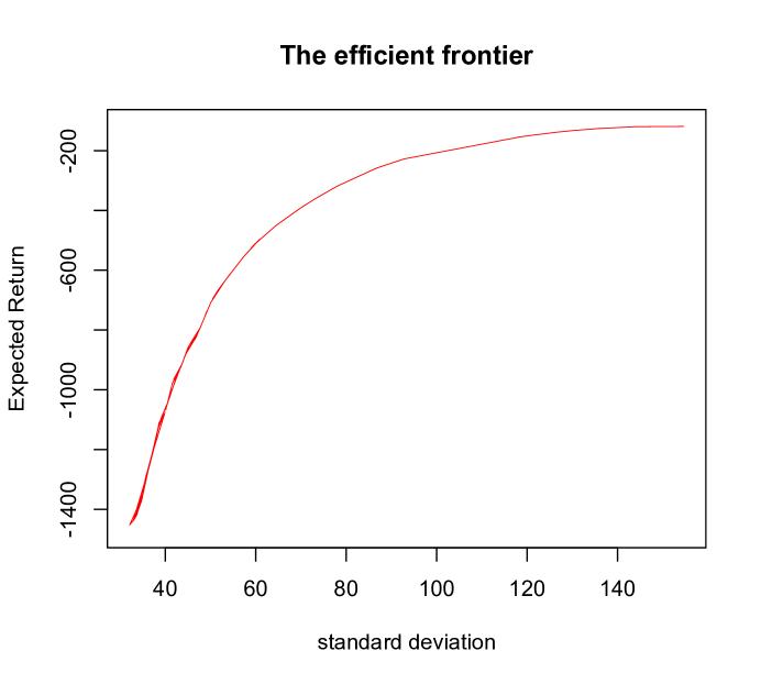
Figure 2: The efficient frontier.

Each point on the frontier represents a distinct strategy for an investor with certain level of risk-aversion. It shows the tradeoff between the expected revenues and the standard deviation. As we can see from this figure, the frontier increases along an approximate smooth concave curve. The slope of the “tangent line” indicates the trader’s risk aversion level $\lambda$.

The point on the most right is obtained for a risk-neutral trader with $\lambda=0$. We define this point as $(Std_{0},R_{0})$. For any other point on the left, we have

$$R_{t}-R_{0}\approx\frac{1}{2}(Std_{t}-Std_{0})^{2}\frac{d^{2}R}{dStd^{2}}\Big{|}_{Std=Std_{0}}.$$

A crucial insight is that for a risk neutral trader, a first-order decrease in the expected revenue can approximately incur a second-order decrease in the standard deviation. The efficient frontier depicted in Figure 2 is consistent with the one for the mean-variance portfolio selection.

3.2.4 Effect of Illiquidity

The cost of trading has three main components, brokerage commission, bid-ask spread (we will discuss this factor later) and price impact, of which liquidity affects the latter two. Brokerage commission is usually negotiable and does not constitute a large fraction of the total cost of trading except in small-size trades, which is a topic beyond the scope of this paper. Stocks with low liquidity can have wide bid-ask spreads. The bid-ask spread, which is the difference between the buying price and the selling price, is incurred as a cost of trading a security. The larger the bid-ask spread, the higher is the cost of trading.

Liquidity also has implications for the price impact of trade. The extent of the price impact depends on the liquidity of the stock. A stock that trades millions of shares a day may be less affected than a stock that trades only a few hundred thousand shares a day. The effect of temporary market impact $\eta^{tem}$, a key indicator of the illiquidity of a market, is shown in Figure 3.

It is clear that traders in a market with larger temporary impact will involve higher transaction costs; and that the cost distribution behaves like a normal distribution under the assumption of constant volatility. We refer interested readers to the analysis of the effects of market impact, both permanently and temporarily, to the work by Almgren [3].

Figure 3: (Left-hand Side): $\eta^{tem}=0.005$;   (Right-hand Side): $\eta^{tem}=0.01$.

4 Stochastic Volatility Model

The constant volatility assumption might be reasonable for large-cap US stocks. However, this assumption becomes defective when we move to the analysis of small and medium-capitalization stocks, whose volatilities vary randomly through the day. In this section, we relax the constant volatility assumption. Thus the value function $J=J(t,s,\sigma,q)$ is a function satisfies HJB-1. Similarly, we consider relaxing the constraints associated with HJB-1 and solve the unconstrained optimization problem in HJB-$1^{\prime}$. We then verify that the obtained optimal control does satisfy all the constraints in HJB-1.

We present a framework that is general enough to take into account the effect of stochastic volatility in the following.

4.1 Slow Mean-reverting Volatility Model

We analyze models in which stock prices are conditionally normal, and the volatility process is a positive and increasing function of a mean-reverting Ornstein-Uhlenbeck (OU) process. That is,

$$\left\{\begin{array}[]{lll}\displaystyle dS_{t}=\phi(\nu_{t})dW_{t}\\ \displaystyle d\nu_{t}=\epsilon(m-\nu_{t})dt+\xi\sqrt{\epsilon}\;dB_{t}\\ B_{t}=\rho W_{t}+\sqrt{1-\rho^{2}}Z_{t}\\ \end{array}\right.$$ (17)

where $\{W_{t}\}$ and $\{Z_{t}\}$ are two independent one-dimensional Brownian motions, and $\rho$ is the correlation between price and volatility shocks, with $|\rho|<1$. The parameter $m$ is the equilibrium or long-term mean, $\epsilon(>0)$ is the intrinsic time-scale of the process, and $\xi$, combining with the scalar $\sqrt{\epsilon}$, represents the degree of volatility around the equilibrium $m$ caused by shocks. Here $\{\nu_{t}\}$ is a simple building-block for a large class of stochastic volatility models described by choice of $\phi(\cdot)$. According to Itô’s lemma,

$$d\phi(\nu_{t})=\epsilon\left[\phi^{\prime}(\nu_{t})(m-\nu_{t})+\xi^{2}\phi^{\prime\prime}(\nu_{t})\right]dt+\xi\phi^{\prime}(\nu_{t})\sqrt{\epsilon}dB_{t}.$$

We call these models mean-reverting because the volatility is a monotonic function of $\{\nu_{t}\}$ whose drift pulls it towards the mean value $m$. The volatility is correspondingly pulled towards approximately $\phi(m)$.

Plenty of analysis on specific Itô models by numerical and analytical methods can be found in the literature [4, 9]. Our goal here is to identify and capture the relevant features of liquidating strategies for small- and medium-capitalization stocks. Our framework in Eq. (17) is adequate and efficient enough to capture this. Here we will work in the regime $\epsilon\ll 1$ (slow mean-reverting). For simplicity, we consider the case of $N=1$. The value function $J$ under this setting solves the following PDE:

$$\left\{\begin{array}[]{lll}\displaystyle\left(\partial_{t}+\mathcal{L}\right)J-\lambda\phi^{2}(\nu)q^{2}+\frac{1}{4\eta^{tem}}(\partial_{q}J+\eta^{per}q)^{2}=0\\ J(T-,s,\nu,q)=-Kq^{2}.\end{array}\right.$$ (18)

Furthermore, we have $J(t,s,\nu,q)=J(t,\nu,q)$ independent of $s$, since the terminal data does not depend on $s$ and PDE (18) introduces no $s$-dependence. Hence, the operator $\mathcal{L}$ takes the form of

$$\mathcal{L}=\epsilon\left((m-\nu)\partial_{\nu}+\frac{1}{2}\xi^{2}\partial_{\nu\nu}\right).$$

Similarly as before, we look for a solution quadratic in the inventory variable $q$

$$J(t,\nu,q)=f(t,\nu)+g(t,\nu)q+h(t,\nu)q^{2}.$$ (19)

The optimal liquidating schedule can then be calculated through the relation

$$\theta^{*}(t,\nu,q)=-\frac{1}{2\eta^{tem}}\big{[}\big{(}2h(t,\nu)+\eta^{per}\big{)}q+g(t,\nu)\big{]}.$$ (20)

To solve Eq. (19), $f,g$ and $h$ must satisfy the following PDEs:

$$\begin{array}[]{lll}\left\{\begin{array}[]{l}\displaystyle(\partial_{t}+\mathcal{L})h-\lambda\phi^{2}(\nu)+\frac{1}{4\eta^{tem}}(2h+\eta^{per})^{2}=0\\ \displaystyle h(T-,\nu)=-K\end{array}\right.\\ \\ \left\{\begin{array}[]{l}\displaystyle(\partial_{t}+\mathcal{L})g+\frac{1}{2\eta^{tem}}(2h+\eta^{per})g=0\\ \displaystyle g(T-,\nu)=0\\ \end{array}\right.\\ \\ \left\{\begin{array}[]{l}\displaystyle(\partial_{t}+\mathcal{L})f+\frac{1}{4\eta^{tem}}g^{2}=0\\ \displaystyle f(T-,\nu)=0.\end{array}\right.\end{array}$$ (21)

It is straightforward to verify that (Feynman-Kac formula)

$$g(t,\nu)\equiv 0\quad\mbox{and}\quad f(t,\nu)\equiv 0.$$

If we set

$$Y_{t}=\frac{1}{2\eta^{tem}}\int_{0}^{t}(2h(u,\nu_{u})+\eta^{per})du\quad{\rm and}\quad\mathfrak{h}(t,\nu_{t},Y_{t})=e^{Y_{t}}(2h(t,\nu_{t})+\eta^{per}).$$

According to Itô’s lemma,

$$\begin{array}[]{lll}d\mathfrak{h}(t,\nu_{t},Y_{t})&=&\displaystyle e^{Y_{t}}\Big{\{}\big{[}2(\partial_{t}+\mathcal{L})h+\frac{1}{2\eta^{tem}}(2h+\eta^{per})^{2}\big{]}dt+2\xi\sqrt{\epsilon}\partial_{\nu}h\;dB_{t}\Big{\}}\\ &=&\displaystyle e^{Y_{t}}\left\{2\lambda\phi^{2}(\nu_{t})dt+2\xi\sqrt{\epsilon}\partial_{\nu}h\;dB_{t}\right\}.\end{array}$$

Applying Itô’s formula to $\mathfrak{h}(u,\nu_{u},Y_{u})$ between $t$ and $T-$, with $h$ satisfying PDE (21), we get:

$$\mathfrak{h}(t,\nu_{t},Y_{t})=e^{Y_{T-}}(-2K+\eta^{per})-2\lambda\int_{t}^{T}e^{Y_{u}}\phi^{2}(\nu_{u})du-2\int_{t}^{T}\xi\sqrt{\epsilon}\partial_{\nu}h(u,\nu_{u})dB_{u}.$$

Hence,

$$\mathfrak{h}(t,\nu,y)=\mathbb{E}\left[e^{Y_{T-}}(-2K+\eta^{per})-2\lambda\int_{t}^{T}e^{Y_{u}}\phi^{2}(\nu_{u})du\Big{|}\nu_{t}=\nu,Y_{t}=y\right].$$ (22)

If condition (14) is satisfied, then $-2K+\eta^{per}<0$, and hence $\mathfrak{h}(t,\nu,y)\leq 0$ for any $(t,\nu,y)\in[0,T)\times\mathbb{R}\times\mathbb{R}$. Therefore, $2h(t,\nu)+\eta^{per}\leq 0$ for any $(t,\nu)\in[0,T)\times\mathbb{R}$. Then the control policy in Eq. (20) is optimal.

Eq. (22) just provides an implicit analytical solution to $\mathfrak{h}$. However, for the general coefficients $(\phi,m,\epsilon,\xi)$, we do not have an explicit solution. The small-$\epsilon$ regime gives rise to a regular perturbation expansion in the powers of $\epsilon$. As in [9], we seek an asymptotic approximation for $h$:

$$h(t,\nu)=h^{(0)}(t,\nu)+\epsilon h^{(1)}(t,\nu)+\epsilon^{2}h^{(2)}(t,\nu)+\cdots+.$$ (23)

This is a series expansion, for which we find $h^{(i)}$ for $i=0,1$ explicitly, and study the accuracy when using the truncated series in Section 4.3.2. In the next sections, we present our asymptotic approach for $h$ and the accuracy of our approximate optimal liquidation policy.

4.2 Asymptotics

We first construct a regular perturbation expansion in the powers of $\epsilon$ by writing

$$\mathcal{L}=\epsilon\mathcal{L}_{0},\quad h(t,\nu)=\sum_{i\geq 0}\epsilon^{i}h^{(i)}(t,\nu)$$

where

$$\mathcal{L}_{0}=(m-\nu)\partial_{\nu}+\frac{1}{2}\xi^{2}\partial_{\nu\nu}.$$

Substituting these expansions into Eq. (21) and grouping the terms of the powers of $\epsilon$, we find that the lowest order equations of the regular perturbation expansion are

$$\begin{array}[]{lll}\mathcal{O}(1):&&\displaystyle\quad\quad\quad\quad 0=\partial_{t}h^{(0)}-\lambda\phi^{2}(\nu)+\frac{1}{4\eta^{tem}}(2h^{(0)}+\eta^{per})^{2}\\ \mathcal{O}(\epsilon):&&\displaystyle\quad\quad\quad\quad 0=\partial_{t}h^{(1)}+\mathcal{L}_{0}h^{(0)}+\frac{1}{\eta^{tem}}(2h^{(0)}+\eta^{per})h^{(1)}\end{array}$$ (24)

with terminal data

$$h^{(0)}(T-,\nu)=-K\quad\mbox{and}\quad h^{(1)}(T-,\nu)=0.$$

The solutions of Eq. (24) can be obtained easily. Indeed, we have

$$\left\{\begin{array}[]{lll}\displaystyle h^{(0)}(t,\nu)=\sqrt{\eta^{tem}\lambda\phi^{2}(\nu)}\cdot\frac{\varsigma(\nu)e^{-2\sqrt{\lambda\phi^{2}(\nu)/\eta^{tem}}(T-t)}-1}{\varsigma(\nu)e^{-2\sqrt{\lambda\phi^{2}(\nu)/\eta^{tem}}(T-t)}+1}-\frac{1}{2}\eta^{per}\\ \displaystyle h^{(1)}(t,\nu)=\int_{t}^{T}D(r;t)\mathcal{L}_{0}h^{(0)}(r,\nu)dr\\ \end{array}\right.$$ (27)

where

$$\varsigma(\nu)=\frac{\sqrt{\eta^{tem}\lambda\phi^{2}(\nu)}-(K-\eta^{per}/2)}{\sqrt{\eta^{tem}\lambda\phi^{2}(\nu)}+(K-\eta^{per}/2)}\quad{\rm and}\quad D(r;t)=\exp\left(\frac{1}{\eta^{tem}}\int_{t}^{r}(2h^{(0)}+\eta^{per})d\tau\right).$$

4.3 Optimal Strategy

We now analyze and interpret how the principle expansion terms for the value function can be used in the expression for the optimal liquidation strategy $\theta^{*}$, which leads to an approximate feedback policy of the form:

$$\theta^{*}(t,\nu,q)=\theta^{(0),*}(t,\nu,q)+\epsilon\;\theta^{(1),*}(t,\nu,q)+\cdots+.$$

4.3.1 Moving-Constant-Volatility Strategy

First, we introduce the zeroth order terms $h^{(0)}$ in the expansion for $h$. This gives the zeroth order optimal liquidation strategy

$$\theta^{(0),*}(t,\nu,q):=-\frac{1}{2\eta^{tem}}\left(2h^{(0)}(t,\nu)+\eta^{per}\right)q.$$

Recall that, in the case of constant volatility approach (Section 3.1),

$$\theta^{Cons}(t,q;\sigma)=-\frac{1}{2\eta^{tem}}\left(2h^{(0)}(t,\nu^{Cons}))+\eta^{per}\right)q,$$ (28)

where $\nu^{Cons}=\phi^{-1}(\sigma)$ is a constant over $[0,T)$. This approximation might be reasonable for most large-cap US stocks, for which, over short-term time frames like one day or less, the volatility can be regard as a constant. However, this might not be a reasonable approximation for assets that are less heavily traded than large-cap US stocks.

The naive constant-approach liquidation strategy for small- and medium-capitalization stocks would adopt the strategy for large-cap US stocks, $\theta^{Cons}$, but with the coefficient $\sigma$ driven by a varying factor $\nu$, i.e.,

$$\theta^{Cons}(t,q;\phi(\nu))=\theta^{(0),*}(t,\nu,q).$$ (29)

We call this strategy the moving constant-approach liquidation strategy. This strategy is a successful one if the parameters remains constant when they are estimated from updated segments of historical data. However, this is not always the case as the risk environment is dynamic.

4.3.2 First-order Correlation to Optimal Policy

The approximation to the optimal strategy can be more accurate by going into the higher order terms. Substituting the expansion of $h$ up to terms in $\epsilon$ gives

$$\theta^{*}(t,\nu,q)=\widetilde{\theta}^{*}(t,\nu,q)+\mbox{higher order terms}$$

where

$$\widetilde{\theta}^{*}(t,\nu,q)=-\frac{1}{2\eta^{tem}}\left(2h^{(0)}(t,\nu)+\eta^{per}\right)q-\frac{\epsilon}{\eta^{tem}}h^{(1)}(t,\nu)q,$$ (30)

and $h^{(0)}$ and $h^{(1)}$ are given by Eq (27).

In Eq.(35), the term with $\epsilon$ corresponds to traders’ response to the risk arising from stochastic volatility, which can be regarded as the principle term hedging the risk factor. In the previous sections, we presented a “pure” stochastic volatility approach to the liquidating problem, in which volatility $\sigma_{t}$ is modeled as an Itô process driven by a Brownian motion that has a component independent of the Brownian motion driving the asset price. In comparison with Almgren’s work in [4], we mainly focus on a special class of volatility model, time-scale volatility model, and worked in the regime $\epsilon\ll 1$. The separation of time-scales with respect to this kind of models provided an efficient way to identify and track the effect of randomly varying volatility. The theorem below justifies the accuracy of this approximation.

Theorem 1

For fixed $t<T$, $\nu$ and $q$, the optimal liquidating strategy $\theta^{*}(t,\nu,q)$ defined in Eq. (20), and our asymptotic approximation $\widetilde{\theta}^{*}(t,\nu,q)$ defined in Eq. (30) satisfy

$$|\theta^{*}(t,\nu,q)-\widetilde{\theta}^{*}(t,\nu,q)|=\mathcal{O}(\epsilon^{2}).$$

Proof: We note that, at any time $t<T$, according to Eqs. (20), (23) and (30)

$$|\theta^{*}(t,\nu,q)-\widetilde{\theta}^{*}(t,\nu,q)|=\frac{|h-(h^{(0)}+\epsilon\;h^{(1)})|}{\eta^{tem}}q.$$

Defining the residual $R^{\epsilon}=h-(h^{(0)}+\epsilon\;h^{(1)})$. It solves the following PDE:

$$\left\{\begin{array}[]{lll}\displaystyle(\partial_{t}+\mathcal{L})R^{\epsilon}+\frac{1}{\eta^{tem}}R^{\epsilon}[h+h^{(0)}+\epsilon h^{(1)}+\eta^{per}]+\epsilon^{2}\left\{\mathcal{L}_{0}h^{(1)}+\frac{1}{\eta^{tem}}(h^{(1)})^{2}\right\}=0\\ R^{\epsilon}(T-,\nu)=0.\end{array}\right.$$

Directly applying the Feynman-Kac formula to this equation yields

$$R^{\epsilon}(t,\nu)=\epsilon^{2}\cdot\mathbb{E}_{t}\int_{t}^{T}D_{2}(r;t)\{\mathcal{L}_{0}h^{(1)}+\frac{1}{\eta^{tem}}(h^{(1)})^{2}\}dr$$ (31)

where

$$D_{2}(r;t)=\exp\left(\frac{1}{\eta^{tem}}\int_{t}^{r}[h+h^{(0)}+\epsilon h^{(1)}+\eta^{per}]d\tau\right).$$

One can see by direct computation that the integrand in Eq. (31) is bounded in $[0,T]$, i.e., there exists a constant $C$, such that $|R^{\epsilon}(t,\nu)|\leq C\epsilon^{2}$ which completes our proof.  

We remark that, given an initial value $\nu_{0}=\nu$,

$$\nu_{t}\big{|}\nu\sim\mathcal{N}\Big{(}m+(\nu-m)e^{-\epsilon t},\;\frac{\xi^{2}}{2}(1-e^{-2\epsilon t})\Big{)},$$

where $\mathcal{N}(\mu,\sigma^{2})$ is the Gaussian distribution with mean $\mu$ and standard variation $\sigma$.

Assume that

$$\sigma_{t}=\phi(\nu_{t})\quad{or}\quad\nu_{t}=\phi^{-1}(\sigma_{t})$$

is observable in real time with some reasonable degree of confidence. Indeed, we cannot observe directly the volatility, what we may observe is the Volatility Index (VIX) which may be used as a proxy for $\sigma_{t}$. There are different techniques to estimate the parameters $(\epsilon,m,\xi)$. These estimators rely on the persistence of market properties (volatility and liquidity), so that information about the past provides reasonable forecasts for the future. Such persistence, at least across short horizons, is well documented (see, for instance, Bouchaud et al. [6] for more details).

4.4 Simulation Results

In this section, we assume $\phi(\nu)=e^{\nu}$ to test the performance of three different strategies on small- and medium-capitalization stocks: (i) constant volatility approach in Eq. (28); (ii) moving constant volatility approach in Eq. (29); and (iii) first-order correction in Eq. (35). We refer to these strategies as “(i) Constant-Vol”, “ (ii) Moving-Constant-Vol” and “(ii) Vol-adjust”, respectively.

As far as our simulation is concerned, we use the following hypothetical values of the model parameters: $\nu=0.5,\ m=1,\ \epsilon=0.01,\ \xi=2,\ \rho=-0.4$. The rest of the parameters are assumed to be the same as those used in Section 3.2. The simulation is obtained through the following procedure: at time t, the trader’s trading rate $\theta_{t}$ is computed, given the state variables. At time $t+dt$, the mid-price is updated by a random increment $\pm e^{\nu}\sqrt{dt}$. The volatility is updated accordingly by a random increment:

$$\epsilon(m-\nu)dt+\xi\sqrt{\epsilon}(\rho\sqrt{dt}\pm\sqrt{1-\rho^{2}}\sqrt{dt})\;\;\mbox{or}\;\;\epsilon(m-\nu)dt+\xi\sqrt{\epsilon}(-\rho\sqrt{dt}\pm\sqrt{1-\rho^{2}}\sqrt{dt}).$$

Figure 4 illustrates the dynamics of the volatility for one simulation path. From the simulation path depicted in Figure 4, we can see the leverage effect between the price and the volatility.

Figure 4: Dynamics of $(S_{t},\exp(\nu_{t}))$ with $\rho=-0.4$.

We then run $1,000$ simulations to compare the performance of these strategies, primarily focusing on the shape of the profit and loss (P&L) profile. The table below shows the final results.

Table 2: 1,000 simulations with $\lambda=0.1$ w.r.t. $\mathcal{R}_{T}$.

Statistics	Constant-Vol	Moving-Constant-Vol	Vol-adjust
Mean	-300.70	-294.50	-288.46
Std	54.76	27.67	27.45
Skewness	1.03	0.23	0.24
Kurtosis	5.26	3.03	3.05
Objective function	-577.58	-565.39	-560.36

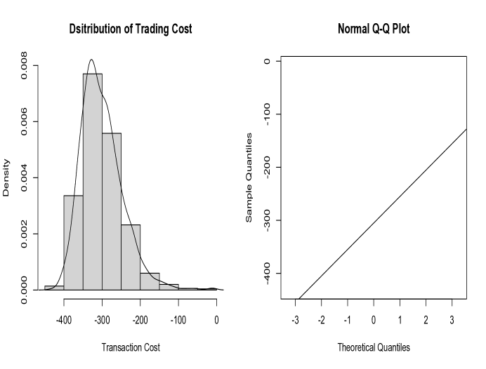
Figure 5: The performance of the “Constant-Vol” strategy on small- and medium-capitalization assets with their volatilities varying randomly through the day.

As we can see from Table 2, the differences among these strategies are significant. Profiting from hedging the risk arising from stochastic volatility is possible. Compared with the “Constant-Vol” strategy, the results in the second column, other strategies adapting to the varying volatility, either “Moving-Constant-Vol” (the results in the third column) or “Vol-adjust” (the results in the fourth column), obtain a lower cost and a smaller risk. The more accurate the adaption, the lower the cost of trading and the smaller the risk of liquidating.

The “Constant-Vol” strategy is a successful one if the underlying assets are large-cap US stocks. However, it is not applicable for assets that are less heavily traded than large-cap US stocks, where volatilities are believed to vary randomly through the day. Figure 5 displays the performance of the “Constant-Vol” strategy on small- and medium-capitalization assets. As we can see from this figure, the distribution of its P & L profile is significantly different from a normal distribution (which is the case for large-cap US stocks) with quite high levels of skewness and kurtosis due to the presence of stochastic volatility effect. Thus at least some adjustment has to be made to identify and capture the relevant characteristics for these assets.

5 An Extension: The Incorporation of Limit Orders

Consider a trader, he/she may submit sell limit orders specifying the quantity and the indicated price per share, which will be executed only when incoming buy market orders are matching with the limit orders. Otherwise, he/she can post sell market orders for an immediate execution, but in this case he/she is going to obtain a less favorable execution price.

Suppose that sell limit orders are submitted at the current best ask, and that the ask-bid spread $\Delta$ keeps unchanged throughout the trading horizon. Moreover, assume that other participants’ buy market orders arrive at Poisson rate $\lambda^{M}=A\exp(-\kappa\Delta)$, a decreasing function of $\Delta$ as in the literature. Let $M_{t}$ count the numbers of buy market orders arriving at the system by time $t$. The number of shares held by the trader, $X_{t}$, can then be expressed by ($N=1$)

$$X_{t}=X_{0}-M_{t}-\int_{0}^{t}\theta_{u}du,\quad X_{0}=Q.$$ (32)

Remark 1

Actually, controls belonging to $\Theta_{t}$ need to satisfy one more condition:

$$\theta_{t}\Big{|}_{dM_{t}=1}=0,$$ (33)

i.e., market order can only be used at times when sell limit orders are not executed. Since for any admissible control process, the integrands in the following two integrals

$$\int_{0}^{t}\mathbb{I}_{\{dM_{u}=0\}}\theta_{u}du\quad\mbox{and}\quad\int_{0}^{t}\theta_{u}du$$

differ at only finitely many times, and when we integrate with respect to the Lebesgue measure $du$, these differences do not matter. Technically speaking, the set of all jumps of the integrand is a countable set, and hence, it has Lebesgue measure zero. Therefore, no mandatory requirement is made to satisfy condition (33) in a continuous-time liquidation setting.

The advantage of market orders over limit orders is that they are less affected by averse price impacts. Suppose a company revises its growth estimates upwards. Those investors who observe piece of this news may react by submitting buy market orders, executed against sell limit orders in the limit order book that have not yet been withdrawn. All these executed sell limit orders may incur opportunity costs due to the adverse selection risk. Market orders, however, will involve unfavorable transaction fees–market impact.

5.1 Adverse Selection

It is possible to incorporate the effect of adverse selection in the trading strategy by assuming that when other participants’ market orders arrive, they may induce a jump in the stock price in the direction of the trade.

Assume that the bid-price satisfies the stochastic differential equation

$$dS^{I}_{t}=\displaystyle dS_{t}+\eta^{u}dM_{t}-\eta^{d}d\hat{M}_{t}-\eta^{per}\theta_{t}dt,$$ (34)

where $\{\hat{M}_{t}\}_{t\geq 0}$ is a jump process satisfying

$$\left\{\begin{array}[]{lll}\mathbb{P}(d\hat{M}_{t}=1|dM_{t}=0)=\frac{\lambda^{M}\eta^{u}}{\eta^{d}}dt\\ \mathbb{P}(d\hat{M}_{t}=1|dM_{t}=1)=0,\end{array}\right.$$ (35)

and $\eta^{u},\eta^{d}>0$ represent the jump in bid-price just after a market order event.

Let us give a brief comment on Eqs. (34) and (35). If bid-side liquidity is found for the order at time $t\in[0,T)$, i.e., $dM_{t}=1$, the expected execution price for the order at time $t$ moves up (by $\eta^{u}$). If no liquidity is found on that side, i.e., $dM_{t}=0$, the expected price move is supposed to be in the opposite direction. By Eq. (35),

$$\begin{array}[]{lll}\displaystyle\mathbb{P}(d\hat{M}_{t}=1)&=&\displaystyle\mathbb{P}(d\hat{M}_{t}=1|dM_{t}=0)\times\mathbb{P}(dM_{t}=0)+\mathbb{P}(d\hat{M}_{t}=1|dM_{t}=1)\times\mathbb{P}(dM_{t}=1)\\ &=&\frac{\lambda^{M}\eta^{u}}{\eta^{d}}dt\times\mathbb{P}(dM_{t}=0)\\ &=&\frac{\lambda^{M}\eta^{u}}{\eta^{d}}dt+o(dt),\end{array}$$ (36)

and

$$\mathbb{P}(d\hat{M}_{t}=0)=1-\frac{\lambda^{M}\eta^{u}}{\eta^{d}}dt+o(dt).$$

Therefore,

$$\begin{array}[]{lll}\mathbb{E}_{t}[\Delta S_{t}^{I}]&=&\mathbb{E}_{t}[S_{t}^{I}-S_{t-}^{I}]\\ &=&[\lambda^{M}dt+o(dt)]\times\eta^{u}-[1-\lambda^{M}dt+o(dt)]\times[\frac{\lambda^{M}\eta^{u}}{\eta^{d}}dt+o(dt)]\times\eta^{d}\\ &=&o(dt).\end{array}$$

To evaluate the effect of the adverse selection on trader’s trading strategy, we consider the simplest case: risk-neutral investors. Similar conclusions may also hold for risk-averse investors.

• For a market-order only trader who does not have any limit orders in the market and simply uses market orders to implement his/her liquidation mandate, we have $\eta^{u}=\eta^{d}=0$. That is, the trader does not use limit orders to “monitor” other participants’ trading behavior, and believes that that stock price evolves over time according to

  $$dS^{I}_{t}=dS_{t}-\eta^{per}\theta_{t}dt.$$

  It is straightforward to verify that the solution to the associated HJB equation is

  $$J(t,q)=\left(\frac{1}{\frac{2}{\eta^{per}-2K}-\frac{1}{\eta^{tem}}(T-t)}-\frac{\eta^{per}}{2}\right)q^{2}.$$

  The optimal liquidating strategy can then be derived through the relations,

  $$\begin{array}[]{ll}\displaystyle\theta^{M}_{t}=-\frac{1}{2\eta^{tem}}\left[\partial_{q}J+\eta^{per}q\right],\\ \displaystyle X_{T}=\frac{\eta^{tem}Q}{\eta^{tem}+T\left(2K-\eta^{per}\right)}.\\ \end{array}$$ (37)

  It is straightforward to verify that if $K$ satisfies Condition (14), then $\theta^{M}_{t}\geq 0,X_{T}\in(0,Q)$, and as $K\to\infty$, $X_{T}\to 0$.

It is the simplest liquidating strategy in limit order books for impatient traders (recall the urgency for liquidation is the primary consideration).

Now let us take limit orders into consideration. In addition to earning ask-bid spreads, limit orders can also be used to incorporate the effect of adverse selection on the trading strategy.

• For a risk-neutral trader who seeks to maximize expected terminal wealth with limit and market orders. Under some smoothness assumptions for a classical solution or the situation when a unique viscosity solution is considered, the value function $J$ without any constraints solves

  $$\left\{\begin{array}[]{lll}\displaystyle\partial_{t}J+\lambda^{M}\left[\eta^{u}+\Delta+J(t,q-1)-J(t,q)\right]\par+\frac{1}{4\eta^{tem}}\left[\partial_{q}J+\eta^{per}q\right]^{2}=0\\ \displaystyle J(T-,q)=-Kq^{2}.\end{array}\right.$$ (38)

  We conjecture that the solution has the following form:

  $$J(t,q)=f(t)+g(t)q+h(t)q^{2}.$$

  Some simple calculations lead to:

  $$\left\{\begin{array}[]{lll}\displaystyle h(t)=\frac{1}{\frac{2}{\eta^{per}-2K}-\frac{1}{\eta^{tem}}(T-t)}-\frac{\eta^{per}}{2}\\ \displaystyle g(t)=-2\lambda^{M}\int_{t}^{T}e^{\frac{1}{2\eta^{tem}}\int_{t}^{r}(2h(\tau)+\eta^{per})d\tau}h(r)dr\\ \displaystyle f(t)=\int_{t}^{T}\Big{[}\lambda^{M}\big{(}\eta^{u}+\Delta+h(r)-g(r)\big{)}+\frac{g^{2}(r)}{4\eta^{tem}}\Big{]}dr,\end{array}\right.$$ (39)

  and

  $$\theta^{M\&L}_{t}=\displaystyle-\frac{1}{2\eta^{tem}}\left[g(t)+\left(2h(t)+\eta^{per}\right)q\right].$$ (40)

  Here $\theta^{M\&L}_{t}$ denotes the optimal liquidating strategy with limit and market orders.

We remark that,

(1)

For any $t\in[0,T)$, $h(t)<0$, $g(t)>0$. Therefore,

$$\theta^{M\&L}_{t}<\theta_{t}^{M}.$$

That is, realizing the information carried by other marker participants (as we assumed in our paper, it is monitored by the execution of limit orders), traders will slow down their liquidating speed so as to get profit from market momentum.

(2)

If condition (14) is satisfied,

$$\begin{array}[]{lll}\displaystyle g(t)&=&\displaystyle-2\lambda^{M}\int_{t}^{T}e^{\frac{1}{2\eta^{tem}}\int_{t}^{r}(2h(\tau)+\eta^{per})d\tau}h(r)dr\\ &=&\displaystyle-2\eta^{tem}\lambda^{M}\bigg{\{}\int_{t}^{T}e^{\frac{1}{2\eta^{tem}}\int_{t}^{r}(2h(\tau)+\eta^{per})d\tau}d\left(\frac{1}{2\eta^{tem}}\int_{t}^{r}(2h(\tau)+\eta^{per})d\tau\right)\\ &&\displaystyle\quad\quad\quad\quad\quad-\frac{\eta^{per}}{2\eta^{tem}}\int_{t}^{T}e^{\frac{1}{2\eta^{tem}}\int_{t}^{r}(2h(\tau)+\eta^{per})d\tau}dr\bigg{\}}\\ &=&\displaystyle-2\eta^{tem}\lambda^{M}\left\{e^{\frac{1}{2\eta^{tem}}\int_{t}^{T}(2h(\tau)+\eta^{per})d\tau}-1-\frac{\eta^{per}}{2\eta^{tem}}\int_{t}^{T}e^{\frac{1}{2\eta^{tem}}\int_{t}^{r}(2h(\tau)+\eta^{per})d\tau}dr\right\}.\end{array}$$

Combining the results in Eq. (39), we have

$$e^{\frac{1}{2\eta^{tem}}\int_{t}^{r}(2h(\tau)+\eta^{per})d\tau}=\frac{\frac{1}{2K-\eta^{per}}+\frac{1}{2\eta^{tem}}(T-r)}{\frac{1}{2K-\eta^{per}}+\frac{1}{2\eta^{tem}}(T-t)}.$$

If the time horizon $T$ satisfies

$$T\leq\frac{2\eta^{tem}}{2K-\eta^{per}}\left[\sqrt{1+\frac{2(2K-\eta^{per})}{\eta^{per}}}-1\right],$$

then $g(t)\leq 2\eta^{tem}\lambda^{M}$ holds for any time $t\in[0,T)$. That is, the reduced liquidation speed $\frac{g(t)}{2\eta^{tem}}$ is always smaller than the rate at which limit sell orders are executed. The overall expected liquidation speed has increased.

(3)

$$\left\{\begin{array}[]{lll}\displaystyle\mathbb{E}[\dot{X}_{t}]=-\lambda^{M}-\mathbb{E}[\theta^{M\&L}_{t}]=-\lambda^{M}+\frac{1}{2\eta^{tem}}\left[g(t)+\left(2h(t)+\eta^{per}\right)\mathbb{E}[X_{t}]\right]\\ \displaystyle X_{0}=Q,\end{array}\right.$$

which yields

$$\mathbb{E}[X_{t}]=Qe^{\frac{1}{2\eta^{tem}}\int_{0}^{t}(2h(\tau)+\eta^{per})d\tau}-\int_{0}^{t}\left[\lambda^{M}-\frac{1}{2\eta^{tem}}g(u)\right]e^{\frac{1}{2\eta^{tem}}\int_{u}^{t}(2h(\tau)+\eta^{per})d\tau}du.$$

The liquidation target

$$Q\geq\max_{t\in[0,T)}e^{-\frac{1}{2\eta^{tem}}\int_{0}^{t}(2h(\tau)+\eta^{per})d\tau}\left[\int_{0}^{t}\left[\lambda^{M}-\frac{1}{2\eta^{tem}}g(u)\right]e^{\frac{1}{2\eta^{tem}}\int_{u}^{t}(2h(\tau)+\eta^{per})d\tau}du-\frac{g(t)}{2h(t)+\eta^{per}}\right],$$

and we have $\mathbb{E}[\theta_{t}^{M\&L}]\geq 0$ and $X_{t}\in[0,Q]$ for any time $t\in[0,T)$. The obtained optimal strategy in Eq. (40) is actually the one we are looking for.

The estimation procedure for the parameter $\lambda_{M}$ in Eq. (39) basically matches the intuition that one must count the number of executions at ask/bid and normalized this quantity by the length of the time horizon. For high-frequency data over $[0,T]$, we have a consistent estimator of $\lambda_{M}$, which is given by

$$\widehat{\lambda}_{M}=\frac{\mbox{\#\{ executions at ask/bid\}}}{T}.$$

5.2 Numerical Results

Consider the situation in which stocks are traded in a single exchange, i.e., $N=1$. As far as our simulation is concerned, we adopt the hypothetical values of the model parameters $\lambda_{M}=100$, $\Delta=0.3$ and $\eta^{u}=\eta^{d}=\eta^{I}=0.02$. Other parameters not listed here are assumed to be the same as those used in Section 3.2. The simulation is obtained through the following procedure:

Table 3: The procedure

Step 0.	Set initial values at time $t=0$;
Step 1.	Compute the trader’s liquidating rate $\theta_{t}$, given the state variables;
Step 2.	If a buy market order arrives at time $t$, then update the quantities by:
	$\left\{\begin{array}[]{l}\displaystyle X_{t+dt}=X_{t}-1\\ \displaystyle C_{t+dt}=C_{t}+(S^{I}_{t}+\Delta)\\ \displaystyle S^{I}_{t+}=S^{I}_{t}+\eta^{I}\end{array}\right.$  execute a trade using sell LOs;
	otherwise,
	$\left\{\begin{array}[]{l}\displaystyle X_{t+dt}=X_{t}-\theta_{t}dt\\ \displaystyle C_{t+dt}=C_{t}+(S^{I}_{t}-\eta^{tem}\theta_{t})\cdot\theta_{t}dt\end{array}\right.$  execute a trade using sell MOs,
	and
	$S^{I}_{t+}=\left\{\begin{array}[]{lll}\displaystyle S^{I}_{t}-\eta^{I}-\eta^{per}\theta_{t}dt,&&\mbox{with probability $\lambda^{M}dt$,}\\ \displaystyle S^{I}_{t}-\eta^{per}\theta_{t}dt,&&\mbox{with probability $1-\lambda^{M}dt$.}\\ \end{array}\right.$
Step 3.	Update the affected price by a random increment $\pm\sigma\sqrt{dt}$:
	$S^{I}_{t+dt}=\left\{\begin{array}[]{lll}S^{I}_{t+}+\sigma\sqrt{dt},&&\mbox{with probability 0.5,}\\ S^{I}_{t+}-\sigma\sqrt{dt},&&\mbox{with probability 0.5;}\\ \end{array}\right.$
Step 4.	Let $t=t+dt$. If $t<T$, return to Step 1; otherwise, stop and exit.

Figures 6 illustrates the dynamics of inventory and affected price for one simulation of a stock path.

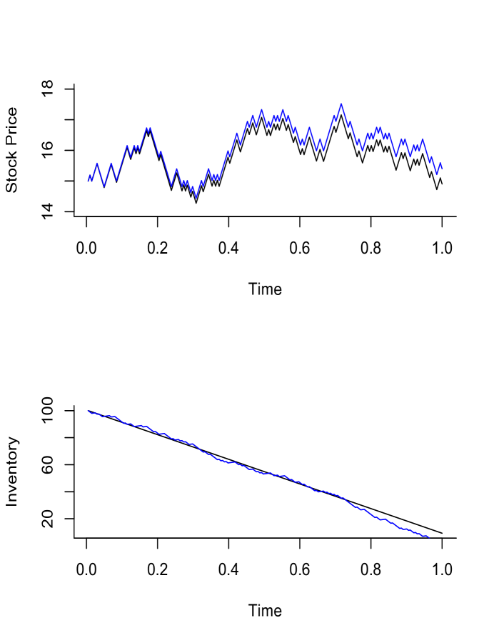
Figure 6: The dynamics of inventory and affected price: (Black) Market orders only; (Blue) Market & limit.

We observe that investors without making use of limit orders would liquidate on a linear trajectory $\theta=\frac{q}{a+b(T-t)}$ and receive a relatively lower execution price from a certain point in time during the trading horizon.

We then run 1000 simulations to investigate the effect of adverse selection on the trading strategy. The performances of strategies aware of this effect and strategies not aware of this effect are depicted in Figure 7.

Figure 7: Profit & Loss profile distributions.

The numerical simulations show that the strategy including the use of limit orders performs better than the market only strategy, it receives a significantly higher expected Profit & Loss profile (from risk-neutral traders’ point of view), say $294.9$ with both MOs and LOs and $-371.3$ with MOs only.

6 Conclusions

In this paper, we utilize a quantitative model to discuss the optimal liquidating problem in an illiquid market. Three different aspects of the optimal liquidation problem are discussed in our paper: (i) optimal liquidating strategy across multiple venues; (ii) optimal liquidating strategy with stochastic volatility (a special case, slow mean-reverting stochastic volatility, was discussed); and (iii) the incorporation of limit orders in optimal liquidation problem.

We formulate the optimal liquidation problem with both temporary and permanent market impacts. Under the no arbitrage assumption, we propose a linear model to determine the equilibrium price in a competitive market with multiple trading venues. Multi-scale analysis method is used to discuss the case of stochastic volatility, where the stochastic volatility is driven by a slow-varying factor $\nu_{t}$. As an extension of our model, we include the use of limit orders. These orders are submitted at the current best ask/bid with buy limit order not being executed. In addition to earn ask-bid spreads, these orders can be used to incorporate the effect of adverse selection on the trading strategy.

In our model, the quantity of limit sell orders is assumed to be one share per trade. Whereas, in reality, it can be multiple shares per trade. This will be an interesting direction for future research.

Appendix

Appendix A.

Proof: In this appendix, we give the steps for deriving HJB-1. Using Eq. (4), the objective at any time $t$ becomes

$$\begin{array}[]{lll}\displaystyle\mathbb{E}_{t}\bigg{[}\int_{t}^{T-}\sigma_{u}X_{u}dW_{u}-\eta^{per}\int_{t}^{T-}X_{u}(\beta^{(1)}_{u}\theta^{(1)}_{u}+\cdots+\beta^{(N)}_{u}\theta^{(N)}_{u})du\\ \displaystyle\quad\quad-\int_{t}^{T-}[\eta^{tem,(1)}(\theta^{(1)}_{u})^{2}+\cdots+\eta^{tem,(N)}(\theta^{(N)}_{u})^{2}]du-\lambda\int_{t}^{T-}\sigma_{u}^{2}X_{u}^{2}du-X_{T-}\mathcal{C}^{o}(X_{T-})\bigg{]}.\end{array}$$

Thus, given initial value $X_{t}=q$,

$$\begin{array}[]{lll}J(t,s,\sigma,q)&=&\displaystyle\max_{\boldsymbol{\theta}(\cdot)\in\Theta_{t}}\;\mathbb{E}^{t,s,\sigma,q}_{\boldsymbol{\theta}(\cdot)}\bigg{[}\int_{t}^{T-}\sigma_{u}X_{u}dW_{u}-\eta^{per}\int_{t}^{T-}X_{u}(\beta^{(1)}_{u}\theta^{(1)}_{u}+\cdots+\beta^{(N)}_{u}\theta^{(N)}_{u})du\\ \displaystyle&&-\int_{t}^{T-}\left([\eta^{tem,(1)}(\theta^{(1)}_{u})^{2}+\cdots+\eta^{tem,(N)}(\theta^{(N)}_{u})^{2}]-\lambda\sigma_{u}^{2}X_{u}^{2}\right)du-X_{T-}\mathcal{C}^{o}(X_{T-})\bigg{]}\\ &=&\displaystyle\max_{\boldsymbol{\theta}(\cdot)\in\Theta_{t}}\;\mathbb{E}^{t,s,\sigma,q}_{\boldsymbol{\theta}(\cdot)}\Bigg{[}\int_{t}^{t+\Delta t}\sigma_{u}X_{u}dW_{u}-\eta^{per}\int_{t}^{t+\Delta t}X_{u}(\beta^{(1)}_{u}\theta^{(1)}_{u}+\cdots+\beta^{(N)}_{u}\theta^{(N)}_{u})du\\ &&\displaystyle-\int_{t}^{t+\Delta t}\left([\eta^{tem,(1)}(\theta^{(1)}_{u})^{2}+\cdots+\eta^{tem,(N)}(\theta^{(N)}_{u})^{2}]-\lambda\sigma_{u}^{2}X_{u}^{2}\right)du\\ &&\displaystyle+\mathbb{E}^{t+\Delta t,s+\Delta s,\sigma+\Delta\sigma,q+\Delta q}_{\boldsymbol{\theta}(\cdot)}\bigg{[}\int_{t+\Delta t}^{T-}\sigma_{u}X_{u}dW_{u}-\eta^{per}\int_{t+\Delta t}^{T-}X_{u}(\beta^{1}_{u}\theta^{(1)}_{u}+\cdots+\beta^{N}_{u}\theta^{(N)}_{u})du\\ &&\displaystyle-\int_{t+\Delta t}^{T-}\left([\eta^{tem,(1)}(\theta^{(1)}_{u})^{2}+\cdots+\eta^{tem,(N)}(\theta^{(N)}_{u})^{2}]-\lambda\sigma_{u}^{2}X_{u}^{2}\right)du-X_{T-}\mathcal{C}^{o}(X_{T-})\bigg{]}\Bigg{]},\\ \end{array}$$

where $\mathbb{E}^{t,s,\sigma,q}_{\boldsymbol{\theta}(\cdot)}[\cdot]$ is the conditional expectation conditioned on the control process $\boldsymbol{\theta}(\cdot)$ and the initial state $(S_{t},\sigma_{t},X_{t})=(s,\sigma,q)$.

Notice that for any control process $\boldsymbol{\theta}(\cdot)\in\Theta_{t}$, we have

$$\begin{array}[]{lll}&&\displaystyle\mathbb{E}^{t+\Delta t,s+\Delta s,\sigma+\Delta\sigma,q+\Delta q}_{\boldsymbol{\theta}(\cdot)}\bigg{[}\int_{t+\Delta t}^{T-}\sigma_{u}X_{u}dW_{u}-\eta^{per}\int_{t+\Delta t}^{T-}X_{u}(\beta^{(1)}_{u}\theta^{(1)}_{u}+\cdots+\beta^{(N)}_{u}\theta^{(N)}_{u})du\\ &&\displaystyle-\int_{t+\Delta t}^{T-}\left([\eta^{tem,(1)}(\theta^{(1)}_{u})^{2}+\cdots+\eta^{tem,(N)}(\theta^{(N)}_{u})^{2}]-\lambda\sigma_{u}^{2}X_{u}^{2}\right)du-X_{T-}\mathcal{C}^{o}(X_{T-})\bigg{]}\\ &=&\displaystyle U(t+\Delta t,s+\Delta s,\sigma+\Delta\sigma,q+\Delta q,\boldsymbol{\theta}(\cdot))\\ &\leq&\displaystyle\max_{\boldsymbol{\theta}(\cdot)\in\Theta_{t+\Delta t}}U(t+\Delta t,s+\Delta s,\sigma+\Delta\sigma,q+\Delta q,\boldsymbol{\theta}(\cdot))\\ &=&\displaystyle J(t+\Delta t,s+\Delta s,\sigma+\Delta\sigma,q+\Delta q).\end{array}$$

Thus, we have

$$\begin{array}[]{lll}J(t,s,\sigma,q)&\leq&\displaystyle\max_{\boldsymbol{\theta}(\cdot)\in\Theta_{t}}\;\mathbb{E}^{t,s,\sigma,q}_{\boldsymbol{\theta}(\cdot)}\Big{[}J(t+\Delta t,s+\Delta s,\sigma+\Delta\sigma,q+\Delta q)+\int_{t}^{t+\Delta t}\sigma_{u}X_{u}dW_{u}\\ &&\displaystyle-\eta^{per}\int_{t}^{t+\Delta t}X_{u}(\beta^{(1)}_{u}\theta^{(1)}_{u}+\cdots+\beta^{(N)}_{u}\theta^{(N)}_{u})du\\ &&\displaystyle-\int_{t}^{t+\Delta t}\left([\eta^{tem,(1)}(\theta^{(1)}_{u})^{2}+\cdots+\eta^{tem,(N)}(\theta^{(N)}_{u})^{2}]-\lambda\sigma_{u}^{2}X_{u}^{2}\right)du\Big{]}.\\ \end{array}$$ (41)

Let $\tilde{\boldsymbol{\theta}}^{*}(\cdot)$ be the optimal control over $[t+\Delta t,T)$, modifying the optimal control between t and $t+\Delta t$ by an arbitrary control $\boldsymbol{\theta}(\cdot)$, i.e. $\boldsymbol{\theta}^{\prime}_{u}=\boldsymbol{\theta}\mathbb{I}_{\{u\leq t+\Delta t\}}+\tilde{\boldsymbol{\theta}}^{*}_{u}\mathbb{I}_{\{u>t+\Delta t\}}$. Then, we obtain

$$\begin{array}[]{lll}J(t,s,\sigma,q)&\geq&J_{\boldsymbol{\theta}^{\prime}(\cdot)}(t,s,\sigma,q)\\ &=&\displaystyle\mathbb{E}^{t,s,\sigma,q}_{\boldsymbol{\theta}(\cdot)}\Big{[}J(t+\Delta t,s+\Delta s,\sigma+\Delta\sigma,q+\Delta q)+\int_{t}^{t+\Delta t}\sigma_{u}X_{u}dW_{u}\\ &&\displaystyle-\eta^{per}\int_{t}^{t+\Delta t}X_{u}(\beta^{(1)}_{u}\theta^{(1)}_{u}+\cdots+\beta^{(N)}_{u}\theta^{(N)}_{u})du\\ &&\displaystyle-\int_{t}^{t+\Delta t}\left([\eta^{tem,(1)}(\theta^{(1)}_{u})^{2}+\cdots+\eta^{tem,(N)}(\theta^{(N)}_{u})^{2}]-\lambda\sigma_{u}^{2}X_{u}^{2}\right)du\Big{]}.\\ \end{array}$$

Hence, we obtain

$$\begin{array}[]{lll}J(t,s,\sigma,q)&\geq&\displaystyle\max_{\boldsymbol{\theta}(\cdot)\in\Theta_{t}}\;\mathbb{E}^{t,s,\sigma,q}_{\boldsymbol{\theta}(\cdot)}\Big{[}J(t+\Delta t,s+\Delta s,\sigma+\Delta\sigma,q+\Delta q)+\int_{t}^{t+\Delta t}\sigma_{u}X_{u}dW_{u}\\ &&\displaystyle-\eta^{per}\int_{t}^{t+\Delta t}X_{u}(\beta^{(1)}_{u}\theta^{(1)}_{u}+\cdots+\beta^{(N)}_{u}\theta^{(N)}_{u})du\\ &&\displaystyle-\int_{t}^{t+\Delta t}\left([\eta^{tem,(1)}(\theta^{(1)}_{u})^{2}+\cdots+\eta^{tem,(N)}(\theta^{(N)}_{u})^{2}]-\lambda\sigma_{u}^{2}X_{u}^{2}\right)du\Big{]}.\\ \end{array}$$ (42)

Putting both inequalities, Eq.(41) and Eq.(42), together, we arrive at the Dynamic Programming Principle (DPP):

$$\begin{array}[]{lll}J(t,s,\sigma,q)&=&\displaystyle\max_{\boldsymbol{\theta}(\cdot)\in\Theta_{t}}\;\mathbb{E}^{t,s,\sigma,q}_{\boldsymbol{\theta}(\cdot)}\Big{[}J(t+\Delta t,s+\Delta s,\sigma+\Delta\sigma,q+\Delta q)+\int_{t}^{t+\Delta t}\sigma_{u}X_{u}dW_{u}\\ &&\displaystyle-\eta^{per}\int_{t}^{t+\Delta t}X_{u}(\beta^{(1)}_{u}\theta^{(1)}_{u}+\cdots+\beta^{(N)}_{u}\theta^{(N)}_{u})du\\ &&\displaystyle-\int_{t}^{t+\Delta t}\left([\eta^{tem,(1)}(\theta^{(1)}_{u})^{2}+\cdots+\eta^{tem,(N)}(\theta^{(N)}_{u})^{2}]-\lambda\sigma_{u}^{2}X_{u}^{2}\right)du\Big{]}.\end{array}$$

Let $\boldsymbol{\theta}^{*}(\cdot)$ be the optimal control over $[t,T)$, then we have

$$\boldsymbol{\theta}^{*}_{t,s,\sigma,q}(t^{\prime},s^{\prime},\sigma^{\prime},q^{\prime})=\tilde{\boldsymbol{\theta}}_{t+\Delta t,s+\Delta s,\sigma+\Delta\sigma,q+\Delta q}^{*}(t^{\prime},s^{\prime},\sigma^{\prime},q^{\prime}),\quad\mbox{for any \; $t^{\prime}>t+\Delta t$}.$$

The dynamic programming equation, HJB equation, is the infinitesimal version of this principle.

Appendix B.

Proof: In the case of (1) $N=1$; or (2) the trading venues have the same market efficiency, $\Delta_{N}=\lambda\sigma^{2}>0$. Hence,

$$h(t;\sigma)=\sqrt{\frac{\Delta_{N}}{a}}\cdot\frac{\varsigma e^{-2\sqrt{a\Delta_{N}}(T-t)}-1}{\varsigma e^{-2\sqrt{a\Delta_{N}}(T-t)}+1}-\frac{\eta^{per}}{2N}.$$

Under the assumption that $K>\displaystyle\frac{b}{2a}+\sqrt{\frac{|\Delta_{N}|}{a}}$, $-1<\varsigma<0$. Therefore, $h$ is a decreasing function in $t$, and for any $n=1,\cdots,N$

$$\begin{array}[]{lll}2h(t;\sigma)+\eta^{per}\beta^{(n)}&=&\displaystyle\sqrt{\frac{\Delta_{N}}{a}}\cdot\frac{\varsigma e^{-2\sqrt{a\Delta_{N}}(T-t)}-1}{\varsigma e^{-2\sqrt{a\Delta_{N}}(T-t)}+1}\leq 0.\end{array}$$ (43)

Recall that

$$\left\{\begin{array}[]{l}\displaystyle\dot{X}_{t}=-\sum_{n=1}^{N}\theta^{n,*}_{t}\\ \displaystyle\theta^{n,*}_{t}=-\frac{1}{2\eta^{tem}}\left[2h(t;\sigma)+\eta^{per}\beta^{(n)}\right]X_{t}.\end{array}\right.$$

Hence, $X_{t}$ satisfies the following first-order ODE:

$$\left\{\begin{array}[]{l}\displaystyle\dot{X}_{t}=\left(\sum_{n=1}^{N}\frac{1}{2\eta^{tem}}\left[2h(t;\sigma)+\eta^{per}\beta^{(n)}\right]\right)X_{t}\\ \displaystyle X_{0}=Q,\end{array}\right.$$

which yields

$$X_{t}=Q\cdot\exp\left(\int_{0}^{t}\sum_{n=1}^{N}\frac{1}{2\eta^{tem}}\left[2h(u;\sigma)+\eta^{per}\beta^{(n)}\right]du\right)\in(0,Q],\quad\mbox{for}\ t\in[0,T).$$ (44)

Combining the results in Eq. (43) and Eq. (44), we conclude that, for any $n=1,\ldots,N$,

$$\theta^{n,*}_{t}=-\frac{1}{2\eta^{tem}}\left[2h(t;\sigma)+\eta^{per}\beta^{(n)}\right]X_{t}\geq 0,$$

and

$$\int_{0}^{T}\sum_{n=1}^{N}\theta^{n,*}_{t}dt=X_{0}-X_{T}=Q\left[1-\exp\left(\int_{0}^{t}\sum_{n=1}^{N}\frac{1}{2\eta^{tem}}\left[2h(u;\sigma)+\eta^{per}\beta^{(n)}\right]du\right)\right]\leq Q.$$

References

- [1] Almgren, R. and Chriss, N. (1999), Value under liquidation, Risk, 12(12):61–63.
- [2] Almgren, R. (2001), Optimal execution of portfolio transactions, Journal of Risk, 3:5–40.
- [3] Almgren, R. (2003), Optimal execution with nonlinear impact functions and trading-enhanced risk, Applied Mathematical Finance, 10(1):1–18.
- [4] Almgren, R. (2012), Optimal Trading with Stochastic Liquidity and Volatility, SIAM Journal on Financial Mathematics, 3, 163–181.
- [5] Brugiere, P. (1996), Optimal portfolio and optimal trading in a dynamic continuous time framework, 6th AFIR Colloquium. Nurenberg, Germany, 12:89.
- [6] Bouchaud, J., Farmer, J. and Lillo, F. (2009), How markets slowly digest changes in supply and demand, in Handbook of Financial Markets: Dynamics and Evolution, North-Holland, San Diego, CA, 57–160.
- [7] Cartea, Á. and Jaimungal, S. (2015), Optimal Execution with limit and market orders, Quantitative Finance, 15(8): 1279–1291.
- [8] Davis, H. and Norman, A. (1990), Portfolio selection with transaction costs, Mathematics of Operations Research, 15(4):676–713.
- [9] Fouque, J., Papanicolaou, G. and Sircar, R. (2000), Mean-reverting stochastic volatility, International Journal of Theoretical and Applied Finance, 3(01): 101–142.
- [10] Fouque, J., Papanicolaou, G., Sircar, R. and Solna, K. (2011), Multiscale stochastic volatility for equity, interest rate, and credit derivatives, Cambridge: Cambridge University Press.
- [11] Tse, S., Forsyth, P., Kennedy, J. and Windcliff, H. (2013), Comparison between the mean-variance optimal and the mean-quadratic-variation optimal trading strategies, Applied Mathematical Finance, 20(5): 415–449.
- [12] Forsyth, P., Kennedy, J., Tse, S. and Windcliff, H. (2012), Optimal trade execution: a mean quadratic variation approach, Journal of Economic Dynamics and Control, 36(12): 1971–1991.
- [13] Gatheral, J. (2010), No-dynamic-arbitrage and market impact, Quantitative Finance, 10:749–759.
- [14] Li, T. and Almgren, R. (2016), Option hedging with smooth market impact, Market Microstructure and Liquidity, 02, 1650002 (26 pages).
- [15] Øksendal, B. (2003), Stochastic Differential Equation, Springer Berlin Heidelberg.
- [16] Øksendal, B. and Sulem, A. (2005), Applied Stochastic Control of Jump Diffusions, Vol. 498, Berlin: Springer.
- [17] Pham, H. (2009), Continuous-time Stochastic Control and Optimization with Financial Applications, Vol. 61, Springer Science & Business Media.
- [18] Rudloff, B., Street, A. and Valladão, D. (2014), Time consistency and risk averse dynamic decision models: Definition, interpretation and practical consequences, European Journal of Operational Research, 234(3): 743–750.
- [19] Soner, H., Shreve, S., and Cvitanić (1994), There is no nontrivial hedging portfolio for option pricing wth transaction costs, Annals of Applied Probability, 5(2):327–355.