Electrical conductivity tensor of dense plasma in magnetic fields

Abstract:

Electrical conductivity of finite-temperature plasma in neutron star crusts is studied for applications in magneto-hydrodynamical description of compact stars. We solve the Boltzmann kinetic equation in relaxation time approximation taking into account the anisotropy of transport due to the magnetic field, the effects of dynamical screening in the scattering matrix element and correlations among the nuclei. We show that conductivity has a minimum at a non-zero temperature, a low-temperature decrease and a power-law increase with increasing temperature. Selected numerical results are shown for matter composed of carbon, iron, and heavier nuclei present in the outer crusts of neutron star.

1 Introduction

Magneto-hydrodynamics (MHD) forms the basis of large-scale description of physics of dense plasma in compact stars. A key quantity in the dissipative formulations of MHD is the conductivity of matter. It determines, for example, the dissipation of currents and therefore the decay of magnetic fields, the dispersion of plasma waves, etc. In turn, magnetic field decay affects the rotational and thermal evolutions of neutron stars and consequently a broad array of their observational manifestations.

Transport in compact star plasma was studied traditionally in the cold (essentially zero-temperature) and dense regime where the constituents form degenerate quantum liquids. This regime is relevant for mature isolated or accreting neutron stars as well as interiors of white dwarfs. The dilute and warm (non-zero temperature) regime is of interest in the context of transient, short-lived states of neutron stars, such as proto-neutron stars newly born in supernova explosions or hypermassive remnants formed in the aftermath of neutron star binary mergers.

We start this article with an overview of the transport calculations of electrical conductivity of compact star matter in the density regime corresponding to their outer crusts ($\rho\leq 10^{11}$ g cm^-3). Then we go on to describe our recent effort to calculate the electrical conductivity of non-zero temperature crustal plasma. We focus on sufficiently high temperatures where nuclei form a liquid coexisting with electronic background of arbitrary degeneracy. We close this review with a summary and outlook. Below we use the natural (Gaussian) units with $\hbar=c=k_{B}=k_{e}=1$, $e=\sqrt{\alpha}$, $\alpha=1/137$ and the metric signature $(1,-1,-1,-1)$.

2 Overview

At densities relevant to interiors of white dwarfs and neutron star crusts the electron-ion system is in a plasma state - the ions are fully ionized while free electrons are the most mobile carriers of charge. By charge conservation electron density is related to the ion charge $Z$ by $n_{e}=Zn_{i}$, where $n_{i}$ is the number density of nuclei. Electrons to a good accuracy form non-interacting gas which becomes degenerate below the Fermi temperature $T_{F}=\varepsilon_{F}-m=(p_{F}^{2}+m^{2})^{1/2}-m$, where the electron Fermi momentum is given by $p_{F}=(3\pi^{2}n_{e})^{1/3}$ and $m$ is the electron mass. The state of ions (mass number $A$ and charge $Z$) is controlled by the value of the Coulomb plasma parameter $\Gamma$

$$\Gamma=\frac{e^{2}Z^{2}}{Ta_{i}}\approx 22.73\frac{Z^{2}}{T_{6}}\bigg{(}\frac{\rho_{6}}{A}\bigg{)}^{1/3},$$ (1)

where $e$ is the elementary charge, $T$ is the temperature, $a_{i}=(4\pi n_{i}/3)^{-1/3}$ is the radius of the spherical volume per ion, $T_{6}$ is the temperature in units $10^{6}$ K and $\rho_{6}$ is the density in units of $10^{6}$ g cm^-3. If $\Gamma\ll 1$ or, equivalently $T\gg T_{\rm C}\equiv Z^{2}e^{2}/a_{i}$, ions form weakly coupled Boltzmann gas. In the regime $\Gamma\geq 1$ ions are strongly coupled and form a liquid for low values of $\Gamma\leq\Gamma_{m}\simeq 160$ and a lattice for $\Gamma>\Gamma_{m}$. The melting temperature of the lattice associated with $\Gamma_{m}$ is defined as $T_{m}=(Ze)^{2}/\Gamma_{m}a_{i}$. For temperatures below the ion plasma temperature

$$T_{p}=\biggl{(}\frac{4\pi Z^{2}e^{2}n_{i}}{M}\biggl{)}^{1/2},$$ (2)

where $M$ is the ion mass, the quantization of oscillations of the lattice becomes important. Figure 1 shows the temperature-density phase diagram of the crustal material in the cases where it is composed of iron $\isotope[56]{Fe}$ (left panel) or carbon $\isotope[12]{C}$ (right panel).

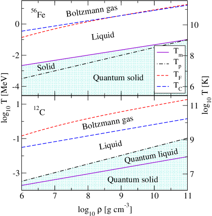
Figure 1: The temperature-density phase diagram of dense plasma composed of iron $\isotope[56]{Fe}$ (upper panel) and carbon $\isotope[12]{C}$ (lower panel). The electron gas degeneracy sets in below the Fermi temperature $T_{F}$ (short dashed lines). The ionic component solidifies below the melting temperature $T_{m}$ (solid lines), while quantum effects become important below the plasma temperature (dash-dotted lines). For temperatures above $T_{\rm C}$ (long dashed lines) the ionic component forms a Boltzmann gas. Note that for $\isotope[12]{C}$ the quantum effects become important in the portion of the phase diagram lying between the lines $T_{p}(\rho)$ and $T_{m}(\rho)$. The present study does not cover the shaded portion of the phase diagram.

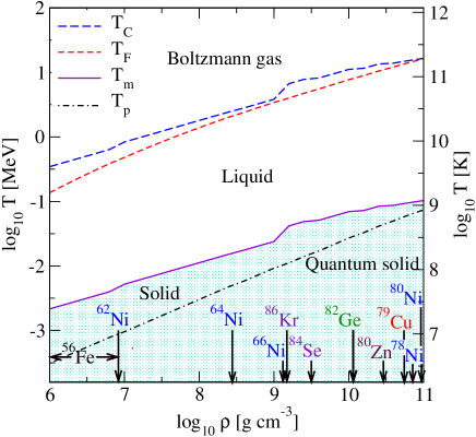
Figure 2: Same as in Fig. 1 but for density dependent composition; for details and references see the discussion in Ref. [12].

While the structure of the phase diagrams for $\isotope[56]{Fe}$ and $\isotope[12]{C}$ are similar there is an important difference as well: as the temperature is lowered the quantum effects become important for carbon prior to solidification, whereas iron solidifies close to the temperature where ionic quantum effects become important. Except of hydrogen and perhaps helium which may not solidify because of quantum zero point motions all heavier elements $Z>2$ solidify at low enough temperature. The phase diagram in the case of density dependent composition is shown in Fig. 2.

The earliest studies of transport in dense matter go back to the work by Mestel, Hoyle [1] and Lee [2] in 1950s, who obtained the “conductive opacity”, or equivalently the thermal conductivity of the electron-ion plasma in non-relativistic electron regime in the context of radiative and thermal transport in white dwarfs. Above densities of the order of $10^{6}$ g cm^-3 electrons are relativistic. Following the initial qualitative estimates of the conductivity of highly compressed matter by Abrikosov in 1963 [3] more detailed calculations were carried out in the 1970s by many authors. In particular the transport in neutron star crusts in the relativistic electron regime was studied in much detail by Flowers and Itoh [4] both in the solid and in the liquid regime using a variational method. They were able to cover a broad range of densities and low-temperature regime including multiple channels of scattering, relatively accurate description of collective modes (phonons) which contribute to the transport coefficients in the solid phase. Their discussion also extended to the neutron drip region where free neutrons contribute to the thermal conductivity and shear viscosity of matter. A critical analysis of the numerical values for the transport coefficients found by different authors was given by Yakovlev and Urpin [5], who also provided useful and simple approximations for the transport coefficients in the degenerate electron regime in terms of the Coulomb logarithm. Nandkumar and Pethick [6] studied the temperature regime above the melting temperature, i.e., where ions form a liquid, showing that the screening of electron-ion interactions can lead to substantial corrections in this case. These calculations agree with those of Itoh et al. [7] who also provide useful fitting formulae for the transport coefficient. Subsequent refinements of the results quoted above included, among other things, multi-phonon process and Debye-Waller factor [8] in the solid phase and improved correlation functions in the liquid phase [9]. The implementation of the transport coefficients of dense matter in the dissipative MHD equations in the case of cold neutron crust plasma in the presence of magnetic fields were discussed by a number of authors [10, 11]. We do not discuss here the physics in ultra-strong fields and confine our attention to non-quantizing fields, i.e., fields below the critical field $B\simeq 10^{14}$ G above which the Landau quantization of electron trajectories becomes important.

3 Formalism

The Boltzmann equation for electron distribution function is given by

$$\frac{\partial f}{\partial t}+{\bm{V}}\frac{\partial f}{\partial\bm{r}}-e(\bm{E}+{\bm{V}}\times\bm{H})\frac{\partial f}{\partial{\bm{p}}}=I[f],$$ (3)

where ${\bm{V}}$ is the electron velocity, ${\bm{E}}$ and ${\bm{H}}$ are the electric and magnetic fields and $I$ is the collision intergal. We are interested in the regime where the collision integral describes electron-ion scattering and, therefore, has the form

$$I[f]=-(2\pi)^{4}\sum\limits_{234}|M_{12\to 34}|^{2}\delta^{(4)}(p+p_{2}-p_{3}-p_{4})[f(1-f_{3})g_{2}-f_{3}(1-f)g_{4}],$$ (4)

where $p_{i}$ are four-momenta of particles, $g$ is the equilibrium distribution function of ions, which to a good accuracy can be described by the Maxwell-Boltzmann distribution with energy spectrum $\varepsilon=p^{2}/2M$, where $M$ is the ion mass. The sum Eq. (4) stands symbolically for the integrals over the phase-space of scattering particles, $M_{12\to 34}$ is the transition matrix element for scattering of relativistic electrons off correlated ions and is given by

$$M_{12\to 34}=\frac{J_{0}J^{\prime}_{0}}{q^{2}+\Pi_{l}(\omega,{\bm{q}})}-\frac{\bm{J}_{t}\bm{J}^{\prime}_{t}}{q^{2}-\omega^{2}+\Pi_{t}(\omega,{\bm{q}})},$$ (5)

where the electron and ion four-currents are given, respectively,

$$J^{\mu}=-e^{*}\bar{u}^{s_{3}}(p_{3})\gamma^{\mu}u^{s}(p),\quad J^{\prime\mu}=Ze^{*}V^{\prime\mu}=Ze^{*}(1,{\bm{p}}^{\prime}/M),$$ (6)

$e^{*}=\sqrt{4\pi}e$, and $J_{t},J^{\prime}_{t}$ are the components of the currents transversal to the moment transfer ${\bm{q}}$, $\Pi_{l}(\omega,{\bm{q}})$ and $\Pi_{t}(\omega,{\bm{q}})$ are the longitudinal and transverse components of the polarization tensor, which describe respectively, the (irreducible) self-energies of longitudinal and transverse photons in the medium (plasma). The form of the matrix element (5) includes thus the dynamical screening of the electron-ion interaction due to the exchange of transverse photons. Such separation has been employed in the treatment of transport in unpaired [13] and superconducting quark matter [14] and we adopt an analogous approach here. We linearize the Boltzmann equation (3) by writing

$$f=f^{0}+\delta f,\quad\delta f=-\Phi\frac{\partial f^{0}}{\partial\varepsilon},$$ (7)

where $f^{0}$ is the equilibrium Fermi-Dirac distribution function, $\delta f\ll f^{0},$ and $\Phi$ is the perturbation. The electric field appears in the drift term of linearized Boltzmann equation at $O(1)$ in perturbation, whereas the term involving magnetic field at order $O(\Phi)$, because $[{\bm{V}}\times{\bm{H}}]({\partial f^{0}}/{\partial{\bm{p}}})\propto[{\bm{V}}\times{\bm{H}}]{\bm{V}}=0.$ We next specify the form of the function $\Phi$ in the case of conduction as $\Phi={\bm{p}}\cdot{\bm{\Xi}}(\varepsilon),$ which after substitution in the linearized Boltzmann equation gives

$$e{\bm{V}}\cdot\left[{\bm{E}}+({\bm{\Xi}}\times{\bm{H}})\right]=-{\bm{\Xi}}\cdot{\bm{p}}~{}\tau^{-1}(\varepsilon),$$ (8)

where the relaxation time, which depends on electron energy $\varepsilon$, is defined by

$$\tau^{-1}(\varepsilon)=(2\pi)^{-5}\int d\omega d\bm{q}\int d\bm{p}_{2}|{M}_{12\to 34}|^{2}\frac{\bm{q}\cdot\bm{p}}{p^{2}}\delta(\varepsilon-\varepsilon_{3}-\omega)\delta(\varepsilon_{2}-\varepsilon_{4}+\omega)g_{2}\frac{1-f^{0}_{3}}{1-f^{0}}.$$ (9)

(Here and below the indices 2 and 4 are reserved for ions, the index 3 corresponds to the outgoing electron). In transforming the linearized collision integral we introduced a dummy integration over energy and momentum transfers, i.e., $\omega=\varepsilon-\varepsilon_{3}$ and ${\bm{q}}={\bm{p}}-{\bm{p}}_{3}$. It remains to express the vector ${\bm{\Xi}}$ describing the perturbation in terms of physical fields; its most general decomposition is given by

$${\bm{\Xi}}=\alpha{\bm{e}}+\beta{\bm{h}}+\gamma[{\bm{e}}\times{\bm{h}}],$$ (10)

where ${\bm{h}}\equiv{\bm{H}}/H$ and ${\bm{e}}\equiv{\bm{E}}/E$ and the coefficients $\alpha$, $\beta$, $\gamma$ are functions of the electron energy. Substituting Eq. (10) in Eq. (8) one finds that $\alpha=-eE\tau/\varepsilon(1+\omega^{2}_{c}\tau^{2})$, $\beta/\alpha=(\omega_{c}\tau)^{2}({\bm{e}}\cdot{\bm{h}})$ and $\gamma/\alpha=-\omega_{c}\tau$, where $\omega_{c}=eH\varepsilon^{-1}$ is the cyclotron frequency. As a result, the most general form of the perturbation is given by

$$\Phi=-\frac{e\tau}{1+(\omega_{c}\tau)^{2}}V_{i}\left[\delta_{ij}-\omega_{c}\tau\varepsilon_{ijk}h_{k}+(\omega_{c}\tau)^{2}h_{i}h_{j}\right]E_{j}.$$ (11)

Using the standard expression for the electrical current in terms of the perturbation $\Phi$ we arrive at the conductivity tensor $\sigma_{ij}=\delta_{ij}\sigma_{0}-\varepsilon_{ijm}h_{m}\sigma_{1}+h_{i}h_{j}\sigma_{2},$ where the components of the tensor are defined as

$$\sigma_{n}=\frac{e^{2}}{3\pi^{2}T}\int_{m}^{\infty}\!\!d\varepsilon\frac{p^{3}}{\varepsilon}\frac{\tau(\omega_{c}\tau)^{n}}{1+(\omega_{c}\tau)^{2}}f^{0}(1-f^{0}),\quad n=0,1,2,$$ (12)

where $T$ is the temperature and the lower bound of the integral is given by the mass of the electron, which vanishes in the ultra-relativistic limit. The conductivity tensor has a particularly simple form if the magnetic field is along the $z$-direction

$$\hat{\sigma}=\begin{pmatrix}\sigma_{0}&-\sigma_{1}&0\\ \sigma_{1}&\sigma_{0}&0\\ 0&0&\sigma\end{pmatrix}.$$ (13)

For zero magnetic field the current is along the electric field and we find the scalar conductivity

$$\sigma=\frac{e^{2}}{3\pi^{2}T}\int_{m}^{\infty}d\varepsilon\frac{p^{3}}{\varepsilon}\tau f^{0}(1-f^{0})=\sigma_{0}+\sigma_{2}.$$ (14)

Thus, the components of the conductivity tensor are fully determined if the relaxation time $\tau$ is known. We evaluate the square of the scattering matrix using the standard QFT methods and then average over the positions of correlated ions, which effectively multiplies the transition probability by the structure function of ions. After some computations we find for the relaxation time

$$\tau^{-1}(\varepsilon) = \frac{\pi Z^{2}e^{4}n_{i}}{\varepsilon p^{3}}\int_{-\infty}^{\varepsilon-m}d\omega e^{-\omega/2T}\frac{f^{0}(\varepsilon-\omega)}{f^{0}(\varepsilon)}\int_{q_{-}}^{q_{+}}dq(q^{2}-\omega^{2}+2\varepsilon\omega)S(q)F^{2}(q)\frac{1}{\sqrt{2\pi}\theta}$$

$$\times e^{-\omega^{2}/2q^{2}\theta^{2}}e^{-q^{2}/8MT}\bigg{\{}\frac{(2\varepsilon-\omega)^{2}-q^{2}}{|q^{2}+\Pi_{l}|^{2}}+\theta^{2}\frac{(q^{2}-\omega^{2})[(2\varepsilon-\omega)^{2}+q^{2}]-4m^{2}q^{2}}{q^{2}|q^{2}-\omega^{2}+\Pi_{t}|^{2}}\bigg{\}},$$

where $S(q)$ is the ionic structure function, $\theta\equiv\sqrt{{T}/{M}}$, $q_{\pm}=|\pm p+\sqrt{p^{2}-(2\omega\epsilon-\omega^{2})}|$ and $\varepsilon=\sqrt{p^{2}+m^{2}}$ for non-interacting electrons. The contribution of longitudinal and transverse photons in (3) separate. The dynamical screening effects contained in the transverse contribution are parametrically suppressed by the factor $T/M$ at low temperatures and for heavy nuclei. This contribution is clearly important in the cases where electron-electron ($e$-$e$) scattering contributes to the collision intergral. This is the case, for example, when ions form a solid lattice and, therefore, Umklapp $e$-$e$ processes are allowed, or in the case of thermal conduction and shear stresses when the $e$-$e$ collisions contribute to the dissipation. Finally, we note that in order to account for the finite size of the nuclei we have multiplied the transition probability in Eq. (3) by the standard expression for the nuclear formfactor [15]

$$F(q)=-3\frac{qr_{c}\cos(qr_{c})-\sin(qr_{c})}{(qr_{c})^{3}},$$ (16)

where $r_{c}$ is the charge radius of the nucleus given by $r_{c}=1.15\,A^{1/3}$ fm.

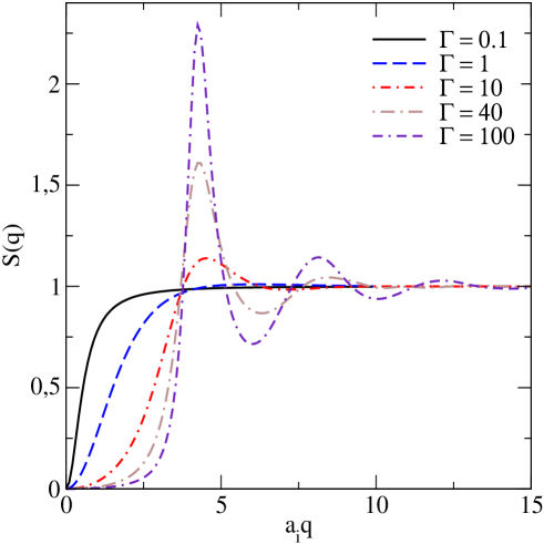
Figure 3: Dependence of the structure function of one-component plasma on the magnitude of momentum transfer $q$ in units of inverse $a_{i}$. For $\Gamma\geq 2$ the structure function is taken from Monte-Carlo calculations of Galam and Hansen [16]. For $\Gamma<2$ we obtain the structure function from the analytical expressions provided by Tamashiro et al. [17].

4 Results

For the numerical computations we need to specify the ion structure function $S(q)$. We assume that only one sort of ions exists at a given density, so that the structure functions of one-component plasma (OCP) can be used. These has been extensively computed using various numerical methods. We adopt the Monte-Carlo results of Galam and Hansen [16] for Coulomb OCP provided in tabular form and set a two-dimension spline function in the space spanned by the magnitude of the momentum transfer $q$ and the plasma parameter $\Gamma$. In the low-$\Gamma$ regime ($\Gamma\leq 2$) we used the analytical (leading order) expressions derived by Tamashiro et al. [17] for Coulomb OCP derived using density functional methods. The resulting structure functions for various values of the plasma parameter $\Gamma$ are shown in Fig. 3 as a function of the dimensionless parameter $a_{i}q$, where $a_{i}$ is the ion-radius as defined after Eq. (1). It is seen that the structure factor universally suppresses the contribution from small-$q$ scattering. The suppression sets in for larger $q$ at larger values of $\Gamma$. The large-$q$ asymptotics is independent of $\Gamma$ as $S(q)\to 1.$ The major difference arises for intermediate values of $q$ where the structure factor oscillates and the amplitude of oscillations increases with the value of $\Gamma$ parameter. The screening of longitudinal and transverse interactions is determined by the corresponding components of the polarization tensor. While expression (3) is exact with respect to the form of the polarization tensor, in the numerical calculations we use the hard-thermal-loop approximation and next-to-leading expansion in $x=\omega/q$. For the real and imaginary parts of the polarization tensor we find

$$\Pi_{l}(q,\omega)=q_{D}^{2}\chi_{l},\qquad\Pi_{t}(q,\omega)=q_{D}^{2}\chi_{t},$$ (17)

where $q_{D}$ is the Debye wave-length and the susceptibilities to order $O(x^{2})$ are given by

$${\rm Re}\chi_{l}(q,\omega)=1-\frac{x^{2}}{\bar{v}^{2}},\quad{\rm Im}\chi_{l}(q,\omega)=-\frac{\pi x}{2\bar{v}},$$ (18)

$${\rm Re}\chi_{t}(q,\omega)=x^{2},\qquad{\rm Im}\chi_{t}(q,\omega)=\frac{\pi}{4}x\bar{v},$$ (19)

where $\bar{v}$ is the electrons average velocity. Because the terms containing $\bar{v}$ are small as well as electrons are ultra-relativistic in the most of the regime of interest we approximate $\bar{v}=1$ in our numerical calculations. For the longitudinal piece of the polarization tensor the screening is finite in the static case $x=0$, while it vanishes for the transverse piece as $\Pi_{t}(q,\omega)\propto x^{2}$, hence the purely dynamical nature of the transverse screening.

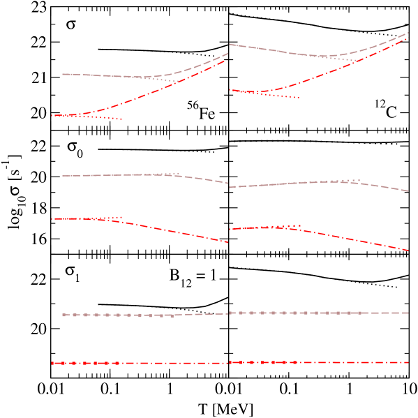
Figure 4: Dependence of the electrical scalar conductivity $\sigma$ (upper panel) and tensor components $\sigma_{0}$ (middle panel) and $\sigma_{1}$ (lower panel) on temperature for three densities log${}_{10}\rho=10$ (solid lines), log${}_{10}\rho=8$ (dashed lines) and log${}_{10}\rho=6$ (dash-dotted lines). The left column contains results for ${}^{56}{\rm Fe}$, the right one for ${}^{12}{\rm C}$. The dotted lines (symbols in the two lower panels) associated with each line show the same, but are evaluate from the zero-temperature Drude formula. The magnetic field is fixed at $B_{12}=1.$

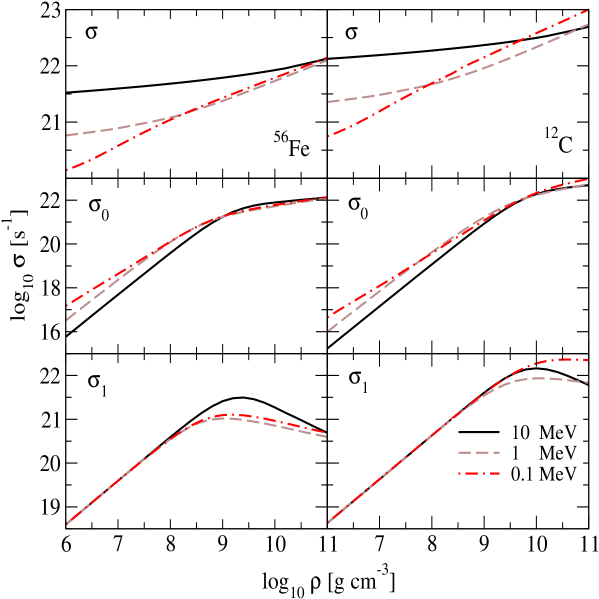
Figure 5: Dependence of the electrical scalar conductivity $\sigma$ (upper panel) and tensor components $\sigma_{0}$ (middle panel) and $\sigma_{1}$ (lower panel) on density for three temperatures $T=10$ MeV (solid lines), $T=1$ MeV (dashed lines) and $T=0.1$ MeV (dash-dotted lines) in the case of ${}^{56}{\rm Fe}$ (left) and $C^{12}{\rm C}$ (right) nuclei and magnetic field $B_{12}=1$.

In the zero-temperature limit Eq. (14) simplifies via the substitution $T\partial f^{0}/\partial\varepsilon=-f^{0}(1-f^{0})\to-T\delta(\varepsilon-\varepsilon_{F})$, i.e.,

$$\sigma=\frac{e^{2}}{3\pi^{2}}\int_{m}^{\infty}d\varepsilon\frac{p^{3}}{\varepsilon}\tau(\varepsilon)\delta(\varepsilon-\varepsilon_{F})=\frac{n_{e}e^{2}\tau_{F}}{\varepsilon_{F}},$$ (20)

where $\tau_{F}$ is the relaxation time (3) taken on the Fermi surface in the $T=0$ limit

$$\tau^{-1}_{F}\equiv\tau^{-1}(\varepsilon_{F})=\frac{4}{3\pi}Ze^{4}\varepsilon_{F}\int_{0}^{2p_{F}}dq\frac{q^{3}}{|q^{2}+\Pi_{l}|^{2}}\bigg{(}1-\frac{q^{2}}{4\varepsilon^{2}_{F}}\bigg{)}S(q)F^{2}(q),$$ (21)

where employed the charge neutrality condition $n_{e}=Zn_{i}$. Neglecting the screening ($\Pi_{l}\to 0$) and the nuclear formfactor [$F(q)\to 1$] we obtain from (21)

$$\tau^{-1}_{F}=\frac{4Ze^{4}\varepsilon_{F}}{3\pi}\int_{0}^{2p_{F}}\frac{dq}{q}\bigg{(}1-\frac{q^{2}}{4\varepsilon^{2}_{F}}\bigg{)}S(q),$$ (22)

which coincides with Eqs. (9) and (11) of Ref. [6].

With the input described above we have evaluated the relaxation time for electron scattering off the ions using Eq. (3) and then the components of the conductivity tensor according to Eq. (12). Here we demonstrate selected results, while our complete results are discussed elsewhere [12]. The conductivity as a function of temperature is shown in Fig. 4 for carbon $\isotope[12]{C}$ and iron $\isotope[56]{Fe}$ nuclei. The magnitude of the magnetic field is fixed to $B_{12}=1$, where $B_{12}$ is the magnetic field in units of $10^{12}$ G. The full results are compared to the case where the conductivity is evaluated from the Drude formula (20), which is shown by dotted lines. The deviation from the zero temperature result are visible for temperatures in the range 0.1$-$1 MeV (MeV = $1.16\times 10^{10}$ K) when the density is varied from $10^{6}$ to $10^{10}$ g cm^-3. It is seen that the $\sigma$ component of conductivity has a minimum as a function of temperature: the low-temperature decrease is replace by a power-law increase with increasing temperature. This increase can be understood in terms of the smearing of the Fermi surface by temperature which makes more electrons available for conduction. The minimum of the conductivity is one of the key findings of our work.

The same as in Fig. 4 but as a function of density for fixed temperature values is shown in Fig. 5. The scalar conductivity and $\sigma_{0}$ component are increasing functions of density and depend strongly on the temperature in the low-density limit, which is associated with lifting of the degeneracy as the temperature is increased. The behaviour of $\sigma_{1}$ is reversed: it is almost independent of temperature and has a maximum. This is the consequence of the different scaling of the components of the conductivity tensor with $\omega_{c}\tau$ parameter, which describes the effects of magnetic field. Our results in the cases of matter composed of $\isotope[12]{C}$ or matter composed of series of nuclei (when the composition varies with density) show the same general trends as for $\isotope[56]{Fe}$. The differences between these cases are quantitative and are discussed in detailed in Ref. [12].

5 Conclusions

In this contribution we gave an overview of our current work on the conductivity of dense matter in the envelopes of neutron stars at non-zero temperature. One ingredient of our effort is the formulation of the transport in a manner which allows us to include the dynamical screening exactly, provided that the polarization tensor of electrons (or equivalently the self-energies of QED photons) in plasma can be computed to desired accuracy. Here we employed the results based on the hard-thermal-loop approximation and low-frequency expansion appropriate at not very high temperatures. We have shown that for electron-ion scattering the dynamical screening is suppressed parametrically by a factor $M/T$, but we anticipate that its effect would be substantial in the cases (a) of high temperatures and presence of light clusters, (b) of low temperatures, where the Umklapp processes with $e$-$e$ scattering are important, (c) of transport processes where $e$-$e$ scattering may be dominant from the outset, such as the thermal conductivity and shear viscosity.

Our numerical results show that the scalar conductivity (no anisotropy due to the $B$-field) has a minimum as a function of temperature, with a power-law decrease at low-temperatures and a power-law increase at higher temperatures. The range of validity of the zero-temperature Drude formula extends from low temperatures up to 0.1$-$1 MeV ($10^{9}-10^{10}$ K), where the lower of these bounds corresponds to density $\rho\sim 10^{6}$ g cm^-3 and the upper one to $\rho\sim 10^{10}$ g cm^-3. The behaviour of the off-diagonal $\sigma_{1}$ component of the conductivity tensor is similar to the one described above except at low densities, where it remains almost constant. Finally the $\sigma_{0}$ component shows strongly density dependent behaviour: for large densities (high degeneracy) it behaves analogous to $\sigma$, but shows the inverse trend for low-densities which is associated with the transition from the regime $\omega_{c}\tau<1$ to $\omega_{c}\tau>1$.

Supplemental material

Below we present numerical tables for the conductivities log${}_{10}\sigma$, log${}_{10}\sigma_{0}$ and log${}_{10}\sigma_{1}$ (in units of s^-1) for various values of magnetic field (in units of $10^{12}$ G) for sets of values of density [g cm^-3] and temperature [MeV]. The tables are provided for three types of composition of matter: $\isotope[12]{C}$ nuclei, $\isotope[56]{Fe}$ nuclei, and density-dependent composition as indicated in Fig. 2. Analytical fits to these results with relative error $\leq 10\%$ can be found in Ref. [12].

Table 1: $\log\sigma$ for $\isotope[12]{C}$

$\log\rho$	$\log T$=-1.0	$\log T$=-0.8	$\log T$=-0.6	$\log T$=-0.4	$\log T$=-0.2	$\log T$=0.0	$\log T$=0.2	$\log T$=0.4	$\log T$=0.6	$\log T$=0.8	$\log T$=1.0
6.0	20.745	20.853	20.973	21.100	21.222	21.356	21.498	21.646	21.798	21.957	22.123
6.2	20.816	20.905	21.013	21.131	21.251	21.378	21.518	21.663	21.814	21.970	22.136
6.4	20.898	20.965	21.057	21.165	21.281	21.401	21.538	21.681	21.830	21.985	22.149
6.6	20.990	21.033	21.106	21.202	21.313	21.426	21.559	21.699	21.846	22.000	22.162
6.8	21.089	21.110	21.163	21.244	21.346	21.452	21.581	21.719	21.864	22.015	22.176
7.0	21.192	21.193	21.226	21.290	21.381	21.482	21.605	21.739	21.882	22.031	22.190
7.2	21.296	21.283	21.296	21.342	21.420	21.518	21.630	21.760	21.900	22.048	22.205
7.4	21.398	21.375	21.372	21.400	21.462	21.553	21.656	21.783	21.920	22.065	22.220
7.6	21.498	21.467	21.452	21.463	21.510	21.589	21.684	21.806	21.940	22.083	22.236
7.8	21.595	21.560	21.535	21.532	21.562	21.629	21.719	21.831	21.961	22.102	22.253
8.0	21.688	21.650	21.620	21.606	21.620	21.672	21.756	21.858	21.984	22.121	22.270
8.2	21.779	21.740	21.705	21.682	21.683	21.720	21.794	21.886	22.008	22.142	22.288
8.4	21.867	21.827	21.789	21.761	21.751	21.773	21.833	21.920	22.033	22.163	22.306
8.6	21.979	21.913	21.874	21.841	21.822	21.831	21.877	21.958	22.059	22.186	22.326
8.8	22.065	21.998	21.958	21.921	21.896	21.893	21.925	21.996	22.088	22.209	22.346
9.0	22.151	22.082	22.041	22.002	21.972	21.959	21.978	22.036	22.121	22.234	22.368
9.2	22.237	22.191	22.124	22.084	22.050	22.029	22.035	22.080	22.159	22.261	22.390
9.4	22.323	22.274	22.207	22.166	22.129	22.102	22.097	22.128	22.198	22.290	22.414
9.6	22.410	22.358	22.289	22.247	22.208	22.177	22.163	22.181	22.238	22.323	22.439
9.8	22.496	22.443	22.396	22.329	22.289	22.254	22.233	22.238	22.282	22.362	22.466
10.0	22.581	22.529	22.479	22.411	22.369	22.332	22.305	22.300	22.330	22.401	22.495
10.2	22.665	22.615	22.563	22.492	22.451	22.411	22.380	22.366	22.383	22.441	22.528
10.4	22.747	22.701	22.648	22.600	22.532	22.492	22.457	22.435	22.441	22.486	22.568
10.6	22.830	22.788	22.734	22.683	22.614	22.573	22.535	22.508	22.503	22.534	22.608
10.8	22.915	22.873	22.821	22.768	22.697	22.654	22.614	22.583	22.569	22.588	22.649
11.0	23.002	22.959	22.910	22.854	22.805	22.737	22.695	22.660	22.639	22.646	22.694

Table 2: $\log\sigma_{0}$ for $\isotope[12]{C}$ at $B_{12}=1$

$\log\rho$	$\log T$=-1.0	$\log T$=-0.8	$\log T$=-0.6	$\log T$=-0.4	$\log T$=-0.2	$\log T$=0.0	$\log T$=0.2	$\log T$=0.4	$\log T$=0.6	$\log T$=0.8	$\log T$=1.0
6.0	16.648	16.551	16.423	16.279	16.132	15.987	15.843	15.696	15.546	15.390	15.227
6.2	16.947	16.878	16.771	16.641	16.503	16.363	16.222	16.078	15.929	15.776	15.613
6.4	17.238	17.195	17.112	16.999	16.871	16.736	16.599	16.458	16.312	16.160	15.999
6.6	17.522	17.504	17.445	17.352	17.236	17.108	16.976	16.838	16.694	16.544	16.385
6.8	17.805	17.806	17.771	17.699	17.597	17.478	17.351	17.216	17.075	16.928	16.770
7.0	18.090	18.104	18.091	18.040	17.955	17.845	17.724	17.594	17.455	17.310	17.155
7.2	18.378	18.402	18.405	18.375	18.307	18.211	18.096	17.970	17.835	17.692	17.539
7.4	18.672	18.702	18.716	18.704	18.655	18.572	18.465	18.345	18.213	18.073	17.923
7.6	18.969	19.003	19.027	19.028	18.997	18.929	18.832	18.718	18.590	18.453	18.306
7.8	19.271	19.307	19.336	19.349	19.333	19.281	19.196	19.089	18.966	18.832	18.688
8.0	19.575	19.613	19.646	19.667	19.664	19.628	19.556	19.457	19.340	19.210	19.069
8.2	19.882	19.921	19.956	19.982	19.990	19.968	19.910	19.821	19.711	19.586	19.448
8.4	20.190	20.229	20.265	20.295	20.310	20.300	20.257	20.179	20.078	19.959	19.826
8.6	20.473	20.535	20.571	20.602	20.622	20.622	20.592	20.530	20.438	20.328	20.201
8.8	20.778	20.837	20.872	20.903	20.925	20.931	20.913	20.865	20.787	20.688	20.570
9.0	21.077	21.133	21.164	21.191	21.213	21.222	21.213	21.180	21.119	21.035	20.929
9.2	21.367	21.399	21.441	21.464	21.481	21.489	21.486	21.466	21.425	21.360	21.272
9.4	21.642	21.669	21.699	21.712	21.722	21.725	21.723	21.713	21.692	21.652	21.589
9.6	21.897	21.915	21.929	21.932	21.931	21.927	21.922	21.918	21.915	21.901	21.869
9.8	22.128	22.132	22.131	22.120	22.108	22.095	22.084	22.081	22.090	22.101	22.101
10.0	22.329	22.320	22.305	22.278	22.257	22.235	22.217	22.210	22.223	22.252	22.280
10.2	22.500	22.480	22.453	22.410	22.382	22.353	22.328	22.316	22.325	22.362	22.410
10.4	22.644	22.616	22.580	22.545	22.491	22.457	22.427	22.408	22.410	22.445	22.506
10.6	22.767	22.735	22.693	22.650	22.590	22.552	22.518	22.492	22.487	22.514	22.577
10.8	22.876	22.842	22.796	22.748	22.682	22.642	22.605	22.574	22.561	22.577	22.634
11.0	22.979	22.940	22.894	22.842	22.796	22.730	22.690	22.655	22.635	22.641	22.687

Table 3: $\log\sigma_{0}$ for $\isotope[12]{C}$ at $B_{12}=10$

$\log\rho$	$\log T$=-1.0	$\log T$=-0.8	$\log T$=-0.6	$\log T$=-0.4	$\log T$=-0.2	$\log T$=0.0	$\log T$=0.2	$\log T$=0.4	$\log T$=0.6	$\log T$=0.8	$\log T$=1.0
6.0	14.648	14.551	14.423	14.280	14.133	13.988	13.842	13.696	13.546	13.390	13.227
6.2	14.948	14.878	14.771	14.642	14.503	14.363	14.221	14.078	13.929	13.776	13.613
6.4	15.238	15.195	15.112	14.999	14.871	14.736	14.599	14.458	14.312	14.160	13.999
6.6	15.523	15.504	15.446	15.352	15.236	15.108	14.975	14.838	14.694	14.544	14.385
6.8	15.806	15.806	15.772	15.700	15.598	15.478	15.351	15.216	15.075	14.928	14.770
7.0	16.090	16.105	16.092	16.041	15.955	15.846	15.724	15.594	15.455	15.310	15.155
7.2	16.379	16.403	16.406	16.376	16.308	16.212	16.096	15.970	15.835	15.692	15.539
7.4	16.672	16.703	16.718	16.705	16.656	16.573	16.466	16.345	16.213	16.073	15.923
7.6	16.970	17.005	17.028	17.031	16.999	16.931	16.833	16.719	16.591	16.454	16.306
7.8	17.273	17.310	17.339	17.353	17.337	17.285	17.199	17.090	16.967	16.833	16.688
8.0	17.579	17.617	17.651	17.673	17.671	17.634	17.561	17.460	17.342	17.212	17.069
8.2	17.888	17.928	17.964	17.992	18.000	17.978	17.920	17.828	17.716	17.589	17.450
8.4	18.199	18.240	18.278	18.310	18.327	18.318	18.274	18.193	18.088	17.965	17.830
8.6	18.487	18.553	18.593	18.628	18.652	18.654	18.623	18.556	18.457	18.340	18.208
8.8	18.801	18.868	18.909	18.946	18.975	18.986	18.969	18.914	18.824	18.713	18.586
9.0	19.115	19.184	19.225	19.264	19.297	19.315	19.309	19.268	19.189	19.085	18.962
9.2	19.429	19.475	19.542	19.582	19.617	19.642	19.645	19.617	19.551	19.454	19.337
9.4	19.742	19.791	19.858	19.899	19.936	19.965	19.977	19.961	19.908	19.820	19.709
9.6	20.055	20.106	20.175	20.215	20.254	20.287	20.305	20.300	20.260	20.182	20.079
9.8	20.368	20.419	20.465	20.531	20.570	20.605	20.628	20.632	20.604	20.540	20.444
10.0	20.680	20.731	20.779	20.844	20.883	20.918	20.945	20.956	20.940	20.889	20.804
10.2	20.993	21.040	21.089	21.154	21.191	21.226	21.255	21.270	21.263	21.226	21.153
10.4	21.304	21.346	21.394	21.436	21.493	21.526	21.553	21.570	21.570	21.545	21.488
10.6	21.610	21.647	21.691	21.732	21.783	21.811	21.835	21.851	21.855	21.839	21.799
10.8	21.907	21.940	21.978	22.015	22.057	22.078	22.095	22.107	22.110	22.101	22.077
11.0	22.192	22.221	22.250	22.278	22.299	22.320	22.328	22.331	22.330	22.325	22.315

Table 4: $\log\sigma_{0}$ for $\isotope[12]{C}$ at $B_{12}=100$

$\log\rho$	$\log T$=-1.0	$\log T$=-0.8	$\log T$=-0.6	$\log T$=-0.4	$\log T$=-0.2	$\log T$=0.0	$\log T$=0.2	$\log T$=0.4	$\log T$=0.6	$\log T$=0.8	$\log T$=1.0
6.0	12.648	12.551	12.423	12.280	12.133	11.988	11.843	11.696	11.546	11.390	11.227
6.2	12.948	12.878	12.771	12.642	12.503	12.363	12.222	12.078	11.929	11.776	11.613
6.4	13.238	13.195	13.112	12.999	12.871	12.736	12.599	12.458	12.312	12.160	11.999
6.6	13.523	13.504	13.446	13.352	13.236	13.108	12.976	12.838	12.694	12.544	12.385
6.8	13.806	13.806	13.772	13.700	13.598	13.478	13.351	13.216	13.075	12.928	12.770
7.0	14.090	14.105	14.092	14.041	13.955	13.846	13.724	13.594	13.455	13.310	13.155
7.2	14.379	14.403	14.406	14.376	14.308	14.212	14.096	13.970	13.835	13.692	13.539
7.4	14.672	14.703	14.718	14.705	14.656	14.573	14.466	14.345	14.213	14.073	13.923
7.6	14.970	15.005	15.028	15.031	14.999	14.931	14.833	14.719	14.591	14.454	14.306
7.8	15.273	15.310	15.339	15.353	15.337	15.285	15.199	15.090	14.967	14.833	14.688
8.0	15.579	15.618	15.651	15.673	15.671	15.634	15.561	15.460	15.342	15.212	15.069
8.2	15.888	15.928	15.964	15.992	16.000	15.979	15.920	15.828	15.716	15.589	15.450
8.4	16.200	16.240	16.278	16.310	16.327	16.319	16.274	16.193	16.088	15.965	15.830
8.6	16.487	16.553	16.593	16.628	16.652	16.655	16.624	16.556	16.457	16.340	16.208
8.8	16.801	16.869	16.909	16.947	16.976	16.987	16.969	16.914	16.825	16.714	16.586
9.0	17.115	17.185	17.226	17.265	17.298	17.316	17.310	17.269	17.190	17.085	16.962
9.2	17.429	17.476	17.543	17.583	17.619	17.644	17.647	17.619	17.553	17.455	17.337
9.4	17.743	17.792	17.860	17.901	17.939	17.969	17.981	17.965	17.911	17.823	17.711
9.6	18.057	18.108	18.178	18.219	18.259	18.292	18.312	18.306	18.266	18.188	18.082
9.8	18.371	18.423	18.470	18.538	18.578	18.614	18.640	18.644	18.616	18.550	18.452
10.0	18.686	18.738	18.788	18.856	18.897	18.935	18.965	18.978	18.962	18.909	18.819
10.2	19.002	19.052	19.104	19.174	19.216	19.256	19.289	19.308	19.303	19.263	19.183
10.4	19.319	19.365	19.419	19.466	19.534	19.575	19.611	19.636	19.641	19.612	19.545
10.6	19.637	19.679	19.732	19.783	19.852	19.893	19.932	19.961	19.974	19.957	19.903
10.8	19.952	19.993	20.045	20.098	20.169	20.211	20.251	20.284	20.303	20.297	20.255
11.0	20.264	20.307	20.356	20.411	20.459	20.527	20.568	20.604	20.629	20.632	20.602

Table 5: $\log\sigma_{1}$ for $\isotope[12]{C}$ at $B_{12}=1$

$\log\rho$	$\log T$=-1.0	$\log T$=-0.8	$\log T$=-0.6	$\log T$=-0.4	$\log T$=-0.2	$\log T$=0.0	$\log T$=0.2	$\log T$=0.4	$\log T$=0.6	$\log T$=0.8	$\log T$=1.0
6.0	18.633	18.633	18.633	18.633	18.629	18.629	18.629	18.629	18.629	18.629	18.629
6.2	18.833	18.833	18.833	18.833	18.831	18.829	18.829	18.829	18.829	18.829	18.829
6.4	19.033	19.033	19.033	19.033	19.032	19.029	19.029	19.029	19.029	19.029	19.029
6.6	19.233	19.233	19.233	19.233	19.233	19.229	19.229	19.229	19.229	19.229	19.229
6.8	19.433	19.433	19.433	19.433	19.433	19.429	19.429	19.429	19.429	19.429	19.429
7.0	19.633	19.633	19.633	19.633	19.633	19.629	19.629	19.629	19.629	19.629	19.629
7.2	19.833	19.833	19.833	19.833	19.833	19.831	19.829	19.829	19.829	19.829	19.829
7.4	20.032	20.032	20.032	20.032	20.032	20.032	20.028	20.029	20.029	20.029	20.029
7.6	20.232	20.232	20.232	20.232	20.232	20.232	20.228	20.228	20.229	20.229	20.229
7.8	20.431	20.431	20.431	20.430	20.430	20.431	20.429	20.428	20.428	20.429	20.429
8.0	20.630	20.629	20.629	20.628	20.628	20.629	20.629	20.626	20.627	20.628	20.628
8.2	20.828	20.827	20.825	20.824	20.824	20.824	20.826	20.824	20.826	20.827	20.828
8.4	21.024	21.022	21.020	21.018	21.017	21.017	21.019	21.020	21.022	21.025	21.027
8.6	21.220	21.215	21.211	21.207	21.204	21.203	21.206	21.212	21.215	21.220	21.224
8.8	21.410	21.402	21.396	21.389	21.383	21.380	21.383	21.393	21.400	21.411	21.418
9.0	21.595	21.582	21.571	21.560	21.549	21.542	21.544	21.557	21.573	21.592	21.606
9.2	21.771	21.757	21.732	21.714	21.696	21.682	21.680	21.697	21.726	21.755	21.782
9.4	21.932	21.910	21.872	21.845	21.817	21.793	21.785	21.802	21.844	21.890	21.938
9.6	22.074	22.040	21.984	21.946	21.906	21.871	21.853	21.867	21.919	21.987	22.060
9.8	22.190	22.142	22.094	22.016	21.964	21.916	21.886	21.892	21.947	22.039	22.137
10.0	22.277	22.215	22.151	22.055	21.993	21.934	21.891	21.884	21.934	22.038	22.162
10.2	22.332	22.261	22.182	22.069	21.999	21.931	21.877	21.855	21.891	21.995	22.137
10.4	22.358	22.284	22.194	22.112	21.990	21.916	21.851	21.815	21.832	21.924	22.078
10.6	22.364	22.289	22.193	22.100	21.971	21.892	21.820	21.771	21.768	21.840	21.990
10.8	22.358	22.281	22.184	22.082	21.945	21.863	21.786	21.726	21.705	21.753	21.887
11.0	22.348	22.265	22.171	22.063	21.968	21.833	21.752	21.684	21.647	21.670	21.781

Table 6: $\log\sigma_{1}$ for $\isotope[12]{C}$ at $B_{12}=10$

$\log\rho$	$\log T$=-1.0	$\log T$=-0.8	$\log T$=-0.6	$\log T$=-0.4	$\log T$=-0.2	$\log T$=0.0	$\log T$=0.2	$\log T$=0.4	$\log T$=0.6	$\log T$=0.8	$\log T$=1.0
6.0	17.633	17.633	17.633	17.633	17.629	17.629	17.629	17.629	17.629	17.629	17.629
6.2	17.833	17.833	17.833	17.833	17.831	17.829	17.829	17.829	17.829	17.829	17.829
6.4	18.033	18.033	18.033	18.033	18.032	18.029	18.029	18.029	18.029	18.029	18.029
6.6	18.233	18.233	18.233	18.233	18.233	18.229	18.229	18.229	18.229	18.229	18.229
6.8	18.433	18.433	18.433	18.433	18.433	18.429	18.429	18.429	18.429	18.429	18.429
7.0	18.633	18.633	18.633	18.633	18.633	18.629	18.629	18.629	18.629	18.629	18.629
7.2	18.833	18.833	18.833	18.833	18.833	18.832	18.829	18.829	18.829	18.829	18.829
7.4	19.033	19.033	19.033	19.033	19.033	19.033	19.029	19.029	19.029	19.029	19.029
7.6	19.233	19.233	19.233	19.233	19.233	19.233	19.229	19.229	19.229	19.229	19.229
7.8	19.433	19.433	19.433	19.433	19.433	19.433	19.431	19.429	19.429	19.429	19.429
8.0	19.633	19.633	19.633	19.633	19.633	19.633	19.633	19.629	19.629	19.629	19.629
8.2	19.833	19.833	19.833	19.833	19.833	19.833	19.833	19.829	19.829	19.829	19.829
8.4	20.033	20.033	20.033	20.033	20.033	20.033	20.033	20.030	20.029	20.029	20.029
8.6	20.233	20.233	20.233	20.233	20.233	20.233	20.233	20.232	20.229	20.229	20.229
8.8	20.433	20.433	20.433	20.433	20.433	20.433	20.433	20.433	20.428	20.429	20.429
9.0	20.633	20.633	20.633	20.632	20.632	20.632	20.632	20.632	20.629	20.628	20.629
9.2	20.833	20.833	20.832	20.832	20.832	20.832	20.831	20.832	20.831	20.828	20.828
9.4	21.032	21.032	21.031	21.031	21.031	21.030	21.030	21.030	21.030	21.027	21.028
9.6	21.231	21.231	21.230	21.229	21.228	21.228	21.227	21.227	21.228	21.226	21.226
9.8	21.430	21.429	21.428	21.426	21.425	21.423	21.422	21.422	21.423	21.424	21.423
10.0	21.628	21.626	21.625	21.621	21.619	21.616	21.614	21.612	21.613	21.617	21.617
10.2	21.824	21.822	21.819	21.813	21.809	21.804	21.799	21.796	21.796	21.801	21.806
10.4	22.017	22.014	22.008	22.003	21.992	21.984	21.975	21.968	21.966	21.973	21.986
10.6	22.206	22.201	22.192	22.182	22.164	22.151	22.136	22.124	22.118	22.125	22.145
10.8	22.388	22.380	22.366	22.349	22.320	22.299	22.276	22.255	22.243	22.248	22.276
11.0	22.560	22.546	22.526	22.499	22.471	22.423	22.390	22.358	22.335	22.336	22.370

Table 7: $\log\sigma_{1}$ for $\isotope[12]{C}$ at $B_{12}=100$

$\log\rho$	$\log T$=-1.0	$\log T$=-0.8	$\log T$=-0.6	$\log T$=-0.4	$\log T$=-0.2	$\log T$=0.0	$\log T$=0.2	$\log T$=0.4	$\log T$=0.6	$\log T$=0.8	$\log T$=1.0
6.0	16.633	16.633	16.633	16.633	16.629	16.629	16.629	16.629	16.629	16.629	16.629
6.2	16.833	16.833	16.833	16.833	16.831	16.829	16.829	16.829	16.829	16.829	16.829
6.4	17.033	17.033	17.033	17.033	17.032	17.029	17.029	17.029	17.029	17.029	17.029
6.6	17.233	17.233	17.233	17.233	17.233	17.229	17.229	17.229	17.229	17.229	17.229
6.8	17.433	17.433	17.433	17.433	17.433	17.429	17.429	17.429	17.429	17.429	17.429
7.0	17.633	17.633	17.633	17.633	17.633	17.629	17.629	17.629	17.629	17.629	17.629
7.2	17.833	17.833	17.833	17.833	17.833	17.832	17.829	17.829	17.829	17.829	17.829
7.4	18.033	18.033	18.033	18.033	18.033	18.033	18.029	18.029	18.029	18.029	18.029
7.6	18.233	18.233	18.233	18.233	18.233	18.233	18.229	18.229	18.229	18.229	18.229
7.8	18.433	18.433	18.433	18.433	18.433	18.433	18.431	18.429	18.429	18.429	18.429
8.0	18.633	18.633	18.633	18.633	18.633	18.633	18.633	18.629	18.629	18.629	18.629
8.2	18.833	18.833	18.833	18.833	18.833	18.833	18.833	18.829	18.829	18.829	18.829
8.4	19.033	19.033	19.033	19.033	19.033	19.033	19.033	19.030	19.029	19.029	19.029
8.6	19.233	19.233	19.233	19.233	19.233	19.233	19.233	19.232	19.229	19.229	19.229
8.8	19.433	19.433	19.433	19.433	19.433	19.433	19.433	19.433	19.429	19.429	19.429
9.0	19.633	19.633	19.633	19.633	19.633	19.633	19.633	19.633	19.630	19.629	19.629
9.2	19.833	19.833	19.833	19.833	19.833	19.833	19.833	19.833	19.832	19.829	19.829
9.4	20.033	20.033	20.033	20.033	20.033	20.033	20.033	20.033	20.033	20.029	20.029
9.6	20.233	20.233	20.233	20.233	20.233	20.233	20.233	20.233	20.233	20.230	20.229
9.8	20.433	20.433	20.433	20.433	20.433	20.433	20.433	20.433	20.433	20.432	20.429
10.0	20.633	20.633	20.633	20.633	20.633	20.633	20.633	20.633	20.633	20.633	20.629
10.2	20.833	20.833	20.833	20.833	20.833	20.833	20.833	20.833	20.833	20.833	20.829
10.4	21.033	21.033	21.033	21.033	21.033	21.033	21.033	21.033	21.033	21.033	21.032
10.6	21.233	21.233	21.233	21.233	21.233	21.232	21.232	21.232	21.232	21.232	21.232
10.8	21.433	21.433	21.433	21.432	21.432	21.432	21.431	21.431	21.431	21.431	21.431
11.0	21.633	21.632	21.632	21.632	21.631	21.631	21.630	21.630	21.629	21.629	21.629

Table 8: $\log\sigma$ for $\isotope[56]{Fe}$

$\log\rho$	$\log T$=-1.0	$\log T$=-0.8	$\log T$=-0.6	$\log T$=-0.4	$\log T$=-0.2	$\log T$=0.0	$\log T$=0.2	$\log T$=0.4	$\log T$=0.6	$\log T$=0.8	$\log T$=1.0
6.0	20.144	20.260	20.375	20.506	20.628	20.762	20.902	21.048	21.200	21.357	21.522
6.2	20.213	20.310	20.413	20.537	20.658	20.785	20.923	21.066	21.216	21.372	21.536
6.4	20.293	20.368	20.456	20.570	20.689	20.809	20.944	21.085	21.233	21.388	21.550
6.6	20.382	20.435	20.517	20.607	20.720	20.834	20.966	21.104	21.250	21.403	21.565
6.8	20.477	20.510	20.572	20.647	20.753	20.861	20.989	21.125	21.268	21.420	21.580
7.0	20.576	20.592	20.634	20.692	20.788	20.889	21.013	21.146	21.287	21.437	21.595
7.2	20.675	20.680	20.702	20.756	20.826	20.925	21.038	21.168	21.307	21.454	21.611
7.4	20.772	20.769	20.777	20.813	20.867	20.961	21.065	21.191	21.327	21.473	21.628
7.6	20.865	20.858	20.856	20.875	20.913	20.997	21.094	21.215	21.348	21.492	21.645
7.8	20.954	20.944	20.937	20.943	20.980	21.036	21.127	21.241	21.370	21.511	21.663
8.0	21.040	21.028	21.019	21.015	21.036	21.079	21.165	21.268	21.394	21.532	21.682
8.2	21.123	21.110	21.099	21.090	21.098	21.125	21.202	21.297	21.418	21.553	21.701
8.4	21.203	21.189	21.177	21.166	21.165	21.192	21.242	21.329	21.444	21.576	21.721
8.6	21.280	21.267	21.254	21.242	21.234	21.249	21.285	21.368	21.471	21.599	21.742
8.8	21.356	21.343	21.329	21.318	21.306	21.310	21.331	21.406	21.500	21.624	21.764
9.0	21.429	21.418	21.404	21.392	21.379	21.375	21.399	21.446	21.532	21.650	21.787
9.2	21.502	21.492	21.479	21.465	21.453	21.443	21.455	21.489	21.572	21.678	21.811
9.4	21.574	21.565	21.552	21.538	21.526	21.514	21.516	21.536	21.610	21.707	21.837
9.6	21.645	21.637	21.625	21.611	21.599	21.586	21.580	21.603	21.651	21.739	21.864
9.8	21.716	21.708	21.698	21.684	21.671	21.658	21.648	21.660	21.694	21.780	21.892
10.0	21.787	21.779	21.770	21.758	21.743	21.731	21.719	21.721	21.742	21.819	21.922
10.2	21.858	21.851	21.842	21.831	21.816	21.804	21.791	21.786	21.810	21.860	21.955
10.4	21.929	21.922	21.914	21.904	21.890	21.876	21.864	21.854	21.867	21.905	21.998
10.6	22.001	21.994	21.986	21.977	21.963	21.949	21.937	21.925	21.929	21.953	22.038
10.8	22.073	22.066	22.058	22.050	22.038	22.023	22.011	21.998	21.995	22.023	22.081
11.0	22.143	22.140	22.132	22.123	22.113	22.099	22.085	22.073	22.065	22.082	22.127

Table 9: $\log\sigma_{0}$ for $\isotope[56]{Fe}$ at $B_{12}=1$

$\log\rho$	$\log T$=-1.0	$\log T$=-0.8	$\log T$=-0.6	$\log T$=-0.4	$\log T$=-0.2	$\log T$=0.0	$\log T$=0.2	$\log T$=0.4	$\log T$=0.6	$\log T$=0.8	$\log T$=1.0
6.0	17.169	17.065	16.945	16.800	16.654	16.512	16.370	16.226	16.078	15.925	15.766
6.2	17.472	17.395	17.295	17.161	17.023	16.886	16.748	16.607	16.460	16.309	16.151
6.4	17.768	17.715	17.637	17.519	17.391	17.258	17.124	16.986	16.842	16.692	16.536
6.6	18.057	18.026	17.957	17.872	17.755	17.629	17.499	17.364	17.223	17.075	16.920
6.8	18.345	18.331	18.285	18.219	18.115	17.997	17.873	17.742	17.603	17.457	17.304
7.0	18.634	18.631	18.605	18.560	18.471	18.362	18.245	18.117	17.982	17.839	17.687
7.2	18.926	18.930	18.919	18.879	18.821	18.725	18.614	18.492	18.360	18.219	18.070
7.4	19.221	19.228	19.228	19.205	19.165	19.082	18.979	18.863	18.736	18.598	18.452
7.6	19.519	19.527	19.533	19.524	19.500	19.432	19.339	19.231	19.109	18.976	18.832
7.8	19.816	19.825	19.833	19.833	19.809	19.771	19.692	19.593	19.479	19.351	19.210
8.0	20.108	20.118	20.126	20.130	20.119	20.093	20.031	19.944	19.840	19.720	19.586
8.2	20.391	20.399	20.405	20.411	20.407	20.394	20.348	20.279	20.189	20.081	19.955
8.4	20.655	20.661	20.665	20.669	20.669	20.657	20.635	20.587	20.518	20.426	20.314
8.6	20.893	20.895	20.897	20.898	20.897	20.892	20.882	20.858	20.814	20.747	20.655
8.8	21.098	21.096	21.094	21.092	21.088	21.086	21.083	21.082	21.066	21.031	20.968
9.0	21.267	21.263	21.257	21.251	21.245	21.241	21.246	21.256	21.268	21.268	21.241
9.2	21.404	21.398	21.390	21.381	21.373	21.365	21.370	21.385	21.421	21.452	21.465
9.4	21.517	21.510	21.501	21.489	21.480	21.469	21.469	21.481	21.531	21.584	21.635
9.6	21.613	21.606	21.596	21.584	21.572	21.561	21.555	21.574	21.610	21.676	21.755
9.8	21.698	21.691	21.681	21.669	21.656	21.644	21.635	21.645	21.674	21.748	21.838
10.0	21.777	21.769	21.761	21.749	21.735	21.723	21.711	21.713	21.732	21.804	21.896
10.2	21.853	21.845	21.837	21.826	21.812	21.799	21.786	21.781	21.805	21.853	21.943
10.4	21.926	21.919	21.911	21.901	21.887	21.873	21.861	21.852	21.864	21.901	21.992
10.6	21.999	21.992	21.984	21.975	21.962	21.948	21.936	21.924	21.927	21.951	22.036
10.8	22.072	22.066	22.057	22.049	22.037	22.023	22.010	21.998	21.994	22.022	22.080
11.0	22.142	22.139	22.132	22.123	22.112	22.098	22.085	22.073	22.064	22.081	22.127

Table 10: $\log\sigma_{0}$ for $\isotope[56]{Fe}$ at $B_{12}=10$

$\log\rho$	$\log T$=-1.0	$\log T$=-0.8	$\log T$=-0.6	$\log T$=-0.4	$\log T$=-0.2	$\log T$=0.0	$\log T$=0.2	$\log T$=0.4	$\log T$=0.6	$\log T$=0.8	$\log T$=1.0
6.0	15.171	15.068	14.948	14.801	14.655	14.512	14.370	14.226	14.078	13.925	13.766
6.2	15.475	15.398	15.298	15.163	15.024	14.886	14.748	14.607	14.460	14.309	14.151
6.4	15.771	15.718	15.641	15.522	15.392	15.259	15.125	14.986	14.842	14.692	14.536
6.6	16.061	16.031	15.961	15.875	15.757	15.630	15.500	15.365	15.223	15.075	14.920
6.8	16.350	16.336	16.290	16.224	16.118	15.999	15.874	15.742	15.603	15.457	15.304
7.0	16.640	16.638	16.612	16.568	16.476	16.366	16.246	16.119	15.983	15.839	15.688
7.2	16.934	16.939	16.929	16.889	16.830	16.731	16.617	16.494	16.361	16.220	16.070
7.4	17.234	17.242	17.243	17.220	17.180	17.093	16.986	16.868	16.739	16.600	16.452
7.6	17.539	17.549	17.556	17.548	17.524	17.452	17.353	17.240	17.115	16.979	16.834
7.8	17.848	17.859	17.870	17.872	17.848	17.806	17.718	17.611	17.490	17.357	17.214
8.0	18.162	18.174	18.186	18.194	18.183	18.156	18.080	17.980	17.864	17.735	17.594
8.2	18.479	18.492	18.504	18.516	18.515	18.502	18.438	18.346	18.236	18.111	17.973
8.4	18.798	18.812	18.824	18.837	18.843	18.826	18.792	18.710	18.606	18.485	18.351
8.6	19.119	19.132	19.145	19.158	19.169	19.163	19.141	19.071	18.974	18.858	18.727
8.8	19.441	19.454	19.467	19.479	19.492	19.494	19.485	19.427	19.338	19.229	19.102
9.0	19.763	19.774	19.787	19.799	19.813	19.820	19.806	19.776	19.697	19.596	19.474
9.2	20.084	20.092	20.105	20.117	20.129	20.140	20.135	20.116	20.051	19.957	19.843
9.4	20.399	20.406	20.417	20.429	20.440	20.451	20.453	20.444	20.392	20.309	20.204
9.6	20.704	20.711	20.719	20.730	20.739	20.749	20.754	20.742	20.715	20.647	20.555
9.8	20.995	21.000	21.006	21.014	21.021	21.028	21.034	21.028	21.012	20.963	20.887
10.0	21.261	21.265	21.268	21.273	21.277	21.281	21.284	21.282	21.273	21.244	21.190
10.2	21.496	21.497	21.498	21.499	21.500	21.500	21.499	21.497	21.493	21.482	21.455
10.4	21.694	21.693	21.691	21.689	21.686	21.682	21.678	21.673	21.673	21.673	21.675
10.6	21.855	21.853	21.849	21.844	21.838	21.831	21.824	21.816	21.815	21.820	21.846
10.8	21.986	21.982	21.977	21.971	21.963	21.953	21.944	21.934	21.930	21.945	21.973
11.0	22.091	22.091	22.085	22.078	22.069	22.058	22.046	22.036	22.028	22.040	22.070

Table 11: $\log\sigma_{0}$ for $\isotope[56]{Fe}$ at $B_{12}=100$

$\log\rho$	$\log T$=-1.0	$\log T$=-0.8	$\log T$=-0.6	$\log T$=-0.4	$\log T$=-0.2	$\log T$=0.0	$\log T$=0.2	$\log T$=0.4	$\log T$=0.6	$\log T$=0.8	$\log T$=1.0
6.0	13.171	13.068	12.948	12.801	12.655	12.512	12.370	12.226	12.078	11.925	11.766
6.2	13.475	13.398	13.298	13.163	13.025	12.886	12.748	12.607	12.460	12.309	12.151
6.4	13.771	13.718	13.641	13.522	13.392	13.259	13.125	12.986	12.842	12.692	12.536
6.6	14.061	14.031	13.961	13.876	13.757	13.630	13.500	13.365	13.223	13.075	12.920
6.8	14.350	14.336	14.290	14.224	14.118	13.999	13.874	13.742	13.603	13.457	13.304
7.0	14.640	14.638	14.612	14.568	14.476	14.366	14.246	14.119	13.983	13.839	13.688
7.2	14.934	14.939	14.929	14.889	14.830	14.731	14.617	14.494	14.361	14.220	14.070
7.4	15.234	15.242	15.243	15.221	15.180	15.093	14.986	14.868	14.739	14.600	14.452
7.6	15.539	15.549	15.557	15.548	15.525	15.452	15.353	15.240	15.115	14.979	14.834
7.8	15.849	15.860	15.871	15.872	15.848	15.806	15.718	15.611	15.490	15.358	15.214
8.0	16.163	16.175	16.186	16.195	16.184	16.157	16.081	15.980	15.864	15.735	15.594
8.2	16.480	16.493	16.505	16.517	16.516	16.503	16.440	16.347	16.236	16.111	15.973
8.4	16.800	16.813	16.826	16.839	16.845	16.828	16.794	16.712	16.607	16.486	16.351
8.6	17.122	17.135	17.149	17.161	17.173	17.166	17.145	17.074	16.976	16.860	16.728
8.8	17.447	17.459	17.473	17.485	17.499	17.501	17.493	17.433	17.343	17.232	17.104
9.0	17.773	17.784	17.798	17.811	17.825	17.833	17.819	17.788	17.707	17.603	17.479
9.2	18.100	18.110	18.124	18.137	18.150	18.163	18.158	18.139	18.070	17.971	17.852
9.4	18.428	18.437	18.450	18.464	18.476	18.491	18.494	18.487	18.428	18.337	18.224
9.6	18.757	18.765	18.776	18.790	18.803	18.817	18.826	18.813	18.783	18.701	18.593
9.8	19.085	19.093	19.103	19.117	19.130	19.144	19.156	19.152	19.133	19.063	18.961
10.0	19.413	19.421	19.430	19.443	19.457	19.469	19.484	19.487	19.479	19.420	19.326
10.2	19.741	19.748	19.757	19.768	19.782	19.795	19.809	19.817	19.803	19.772	19.687
10.4	20.067	20.074	20.082	20.092	20.105	20.119	20.132	20.143	20.138	20.118	20.044
10.6	20.391	20.397	20.405	20.414	20.426	20.440	20.451	20.464	20.466	20.456	20.394
10.8	20.710	20.716	20.723	20.731	20.742	20.755	20.766	20.779	20.785	20.769	20.734
11.0	21.007	21.028	21.034	21.042	21.050	21.062	21.073	21.083	21.092	21.084	21.059

Table 12: $\log\sigma_{1}$ for $\isotope[56]{Fe}$ at $B_{12}=1$

$\log\rho$	$\log T$=-1.0	$\log T$=-0.8	$\log T$=-0.6	$\log T$=-0.4	$\log T$=-0.2	$\log T$=0.0	$\log T$=0.2	$\log T$=0.4	$\log T$=0.6	$\log T$=0.8	$\log T$=1.0
6.0	18.600	18.601	18.601	18.601	18.597	18.596	18.597	18.597	18.597	18.597	18.597
6.2	18.800	18.800	18.801	18.801	18.798	18.796	18.797	18.797	18.797	18.797	18.797
6.4	18.999	19.000	19.000	19.000	18.999	18.996	18.996	18.997	18.997	18.997	18.997
6.6	19.199	19.199	19.199	19.200	19.200	19.196	19.196	19.197	19.197	19.197	19.197
6.8	19.398	19.398	19.398	19.399	19.399	19.396	19.396	19.396	19.397	19.397	19.397
7.0	19.596	19.596	19.596	19.597	19.598	19.595	19.596	19.596	19.596	19.597	19.597
7.2	19.793	19.793	19.793	19.794	19.795	19.796	19.794	19.795	19.796	19.796	19.796
7.4	19.988	19.988	19.988	19.989	19.990	19.993	19.992	19.994	19.995	19.996	19.996
7.6	20.181	20.180	20.179	20.179	20.181	20.186	20.186	20.190	20.193	20.195	20.196
7.8	20.368	20.366	20.365	20.364	20.367	20.372	20.378	20.384	20.389	20.392	20.394
8.0	20.547	20.544	20.541	20.539	20.541	20.547	20.560	20.570	20.580	20.587	20.591
8.2	20.712	20.707	20.702	20.697	20.697	20.702	20.724	20.742	20.762	20.776	20.785
8.4	20.856	20.848	20.841	20.833	20.829	20.841	20.861	20.893	20.927	20.954	20.972
8.6	20.972	20.961	20.949	20.939	20.929	20.938	20.961	21.014	21.065	21.111	21.145
8.8	21.052	21.038	21.022	21.008	20.994	20.996	21.016	21.087	21.162	21.237	21.296
9.0	21.095	21.080	21.060	21.042	21.024	21.017	21.050	21.110	21.210	21.319	21.412
9.2	21.105	21.089	21.067	21.045	21.025	21.010	21.031	21.088	21.211	21.347	21.481
9.4	21.089	21.074	21.052	21.027	21.005	20.984	20.991	21.033	21.165	21.321	21.495
9.6	21.057	21.041	21.020	20.994	20.970	20.947	20.940	20.989	21.087	21.252	21.457
9.8	21.014	20.997	20.979	20.952	20.926	20.903	20.885	20.914	20.993	21.166	21.376
10.0	20.964	20.947	20.930	20.905	20.877	20.854	20.831	20.841	20.894	21.060	21.269
10.2	20.910	20.895	20.878	20.855	20.827	20.802	20.778	20.772	20.830	20.947	21.148
10.4	20.854	20.840	20.823	20.803	20.776	20.749	20.725	20.709	20.743	20.836	21.038
10.6	20.798	20.785	20.768	20.750	20.724	20.696	20.673	20.651	20.665	20.730	20.920
10.8	20.744	20.731	20.715	20.697	20.674	20.645	20.620	20.597	20.595	20.664	20.803
11.0	20.693	20.678	20.663	20.645	20.624	20.596	20.569	20.546	20.534	20.579	20.692

Table 13: $\log\sigma_{1}$ for $\isotope[56]{Fe}$ at $B_{12}=10$

$\log\rho$	$\log T$=-1.0	$\log T$=-0.8	$\log T$=-0.6	$\log T$=-0.4	$\log T$=-0.2	$\log T$=0.0	$\log T$=0.2	$\log T$=0.4	$\log T$=0.6	$\log T$=0.8	$\log T$=1.0
6.0	17.601	17.601	17.601	17.601	17.597	17.596	17.597	17.597	17.597	17.597	17.597
6.2	17.801	17.801	17.801	17.801	17.799	17.796	17.797	17.797	17.797	17.797	17.797
6.4	18.001	18.001	18.001	18.001	18.000	17.996	17.997	17.997	17.997	17.997	17.997
6.6	18.201	18.201	18.201	18.201	18.201	18.196	18.197	18.197	18.197	18.197	18.197
6.8	18.401	18.401	18.401	18.401	18.401	18.396	18.397	18.397	18.397	18.397	18.397
7.0	18.601	18.601	18.601	18.601	18.601	18.596	18.597	18.597	18.597	18.597	18.597
7.2	18.801	18.801	18.801	18.801	18.801	18.799	18.797	18.797	18.797	18.797	18.797
7.4	19.001	19.001	19.001	19.001	19.001	19.001	18.997	18.997	18.997	18.997	18.997
7.6	19.201	19.201	19.201	19.201	19.201	19.201	19.196	19.197	19.197	19.197	19.197
7.8	19.401	19.401	19.401	19.401	19.401	19.401	19.398	19.396	19.397	19.397	19.397
8.0	19.601	19.600	19.601	19.601	19.601	19.601	19.600	19.596	19.596	19.597	19.597
8.2	19.800	19.800	19.800	19.800	19.800	19.800	19.800	19.796	19.796	19.796	19.797
8.4	19.999	19.999	19.999	19.999	19.999	19.999	19.999	19.996	19.996	19.996	19.996
8.6	20.198	20.198	20.198	20.198	20.197	20.197	20.198	20.197	20.195	20.196	20.196
8.8	20.396	20.396	20.395	20.395	20.394	20.394	20.394	20.396	20.393	20.394	20.395
9.0	20.592	20.591	20.591	20.590	20.589	20.589	20.589	20.590	20.589	20.592	20.594
9.2	20.784	20.784	20.782	20.781	20.780	20.779	20.779	20.780	20.784	20.786	20.790
9.4	20.971	20.970	20.968	20.966	20.964	20.962	20.961	20.961	20.969	20.974	20.983
9.6	21.148	21.146	21.144	21.140	21.136	21.132	21.130	21.133	21.140	21.152	21.168
9.8	21.310	21.307	21.303	21.297	21.291	21.285	21.279	21.281	21.289	21.314	21.339
10.0	21.448	21.443	21.437	21.429	21.419	21.411	21.401	21.399	21.406	21.445	21.486
10.2	21.553	21.547	21.539	21.529	21.515	21.502	21.489	21.481	21.500	21.536	21.599
10.4	21.622	21.614	21.604	21.592	21.574	21.557	21.541	21.527	21.541	21.582	21.673
10.6	21.655	21.646	21.633	21.620	21.600	21.579	21.560	21.542	21.547	21.584	21.697
10.8	21.658	21.648	21.634	21.620	21.600	21.575	21.554	21.533	21.529	21.580	21.677
11.0	21.642	21.629	21.616	21.600	21.581	21.555	21.530	21.509	21.496	21.533	21.624

Table 14: $\log\sigma_{1}$ for $\isotope[56]{Fe}$ at $B_{12}=100$

$\log\rho$	$\log T$=-1.0	$\log T$=-0.8	$\log T$=-0.6	$\log T$=-0.4	$\log T$=-0.2	$\log T$=0.0	$\log T$=0.2	$\log T$=0.4	$\log T$=0.6	$\log T$=0.8	$\log T$=1.0
6.0	16.601	16.601	16.601	16.601	16.597	16.596	16.597	16.597	16.597	16.597	16.597
6.2	16.801	16.801	16.801	16.801	16.799	16.796	16.797	16.797	16.797	16.797	16.797
6.4	17.001	17.001	17.001	17.001	17.000	16.996	16.997	16.997	16.997	16.997	16.997
6.6	17.201	17.201	17.201	17.201	17.201	17.196	17.197	17.197	17.197	17.197	17.197
6.8	17.401	17.401	17.401	17.401	17.401	17.396	17.397	17.397	17.397	17.397	17.397
7.0	17.601	17.601	17.601	17.601	17.601	17.596	17.597	17.597	17.597	17.597	17.597
7.2	17.801	17.801	17.801	17.801	17.801	17.799	17.797	17.797	17.797	17.797	17.797
7.4	18.001	18.001	18.001	18.001	18.001	18.001	17.997	17.997	17.997	17.997	17.997
7.6	18.201	18.201	18.201	18.201	18.201	18.201	18.197	18.197	18.197	18.197	18.197
7.8	18.401	18.401	18.401	18.401	18.401	18.401	18.398	18.397	18.397	18.397	18.397
8.0	18.601	18.601	18.601	18.601	18.601	18.601	18.600	18.597	18.597	18.597	18.597
8.2	18.801	18.801	18.801	18.801	18.801	18.801	18.801	18.797	18.797	18.797	18.797
8.4	19.001	19.001	19.001	19.001	19.001	19.001	19.001	18.997	18.997	18.997	18.997
8.6	19.201	19.201	19.201	19.201	19.201	19.201	19.201	19.200	19.197	19.197	19.197
8.8	19.401	19.401	19.401	19.401	19.401	19.401	19.401	19.401	19.397	19.397	19.397
9.0	19.601	19.601	19.601	19.601	19.601	19.601	19.601	19.601	19.597	19.597	19.597
9.2	19.801	19.801	19.801	19.801	19.801	19.801	19.801	19.801	19.800	19.797	19.797
9.4	20.001	20.001	20.001	20.001	20.001	20.001	20.001	20.001	20.001	19.996	19.997
9.6	20.201	20.201	20.201	20.200	20.200	20.200	20.200	20.200	20.200	20.196	20.196
9.8	20.400	20.400	20.400	20.400	20.400	20.400	20.400	20.400	20.400	20.399	20.396
10.0	20.599	20.599	20.599	20.599	20.599	20.599	20.599	20.599	20.599	20.599	20.595
10.2	20.798	20.798	20.798	20.797	20.797	20.797	20.797	20.796	20.797	20.797	20.794
10.4	20.995	20.995	20.995	20.994	20.994	20.993	20.993	20.993	20.993	20.993	20.994
10.6	21.190	21.190	21.190	21.189	21.188	21.187	21.187	21.186	21.185	21.186	21.189
10.8	21.382	21.381	21.381	21.380	21.379	21.377	21.376	21.374	21.373	21.374	21.377
11.0	21.558	21.566	21.565	21.564	21.562	21.559	21.557	21.554	21.551	21.553	21.556

Table 15: $\log\sigma$ for density-dependent composition

$\log\rho$	$\log T$=-1.0	$\log T$=-0.8	$\log T$=-0.6	$\log T$=-0.4	$\log T$=-0.2	$\log T$=0.0	$\log T$=0.2	$\log T$=0.4	$\log T$=0.6	$\log T$=0.8	$\log T$=1.0
6.0	20.144	20.260	20.376	20.506	20.628	20.762	20.902	21.048	21.200	21.357	21.522
6.2	20.213	20.310	20.413	20.537	20.658	20.785	20.923	21.066	21.216	21.372	21.536
6.4	20.293	20.368	20.456	20.570	20.689	20.809	20.944	21.085	21.233	21.388	21.550
6.6	20.382	20.435	20.517	20.607	20.720	20.834	20.966	21.104	21.250	21.403	21.565
6.8	20.477	20.510	20.572	20.647	20.753	20.861	20.989	21.125	21.268	21.420	21.580
7.0	20.536	20.555	20.598	20.671	20.755	20.857	20.981	21.114	21.256	21.406	21.565
7.2	20.633	20.641	20.666	20.721	20.792	20.893	21.006	21.136	21.276	21.424	21.581
7.4	20.730	20.730	20.740	20.777	20.833	20.928	21.033	21.160	21.296	21.442	21.598
7.6	20.823	20.817	20.819	20.839	20.893	20.964	21.062	21.184	21.317	21.461	21.615
7.8	20.912	20.903	20.899	20.907	20.944	21.003	21.094	21.209	21.339	21.481	21.633
8.0	20.998	20.987	20.980	20.979	21.001	21.044	21.132	21.236	21.363	21.501	21.652
8.2	21.080	21.068	21.059	21.053	21.063	21.105	21.169	21.265	21.387	21.523	21.671
8.4	21.160	21.147	21.136	21.128	21.129	21.157	21.208	21.296	21.412	21.545	21.691
8.6	21.232	21.220	21.207	21.198	21.193	21.209	21.248	21.332	21.438	21.567	21.711
8.8	21.307	21.296	21.283	21.273	21.264	21.270	21.308	21.370	21.466	21.592	21.733
9.0	21.380	21.371	21.358	21.346	21.337	21.334	21.360	21.409	21.497	21.617	21.756
9.2	21.311	21.304	21.297	21.288	21.282	21.284	21.302	21.353	21.428	21.540	21.679
9.4	21.382	21.375	21.369	21.360	21.352	21.351	21.362	21.400	21.465	21.569	21.704
9.6	21.478	21.472	21.465	21.455	21.446	21.442	21.445	21.472	21.539	21.621	21.751
9.8	21.549	21.543	21.536	21.527	21.517	21.511	21.511	21.528	21.581	21.659	21.779
10.0	21.619	21.614	21.606	21.599	21.589	21.580	21.579	21.588	21.628	21.698	21.809
10.2	21.717	21.712	21.704	21.696	21.686	21.675	21.670	21.673	21.702	21.761	21.863
10.4	21.787	21.782	21.776	21.768	21.758	21.747	21.741	21.739	21.758	21.817	21.903
10.6	21.888	21.883	21.876	21.868	21.858	21.846	21.837	21.831	21.841	21.888	21.967
10.8	21.976	21.970	21.964	21.955	21.946	21.933	21.922	21.915	21.917	21.952	22.021
11.0	-	22.055	22.049	22.040	22.031	22.018	22.006	21.997	21.994	22.019	22.076

Table 16: $\log\sigma_{0}$ for density-dependent composition at $B_{12}=1$

$\log\rho$	$\log T$=-1.0	$\log T$=-0.8	$\log T$=-0.6	$\log T$=-0.4	$\log T$=-0.2	$\log T$=0.0	$\log T$=0.2	$\log T$=0.4	$\log T$=0.6	$\log T$=0.8	$\log T$=1.0
6.0	17.169	17.065	16.945	16.800	16.654	16.512	16.370	16.226	16.078	15.925	15.765
6.2	17.472	17.395	17.294	17.161	17.023	16.885	16.748	16.607	16.460	16.309	16.151
6.4	17.768	17.715	17.637	17.519	17.390	17.258	17.124	16.986	16.842	16.692	16.536
6.6	18.057	18.026	17.957	17.872	17.754	17.628	17.499	17.364	17.223	17.075	16.920
6.8	18.345	18.331	18.285	18.219	18.115	17.997	17.873	17.741	17.603	17.457	17.304
7.0	18.650	18.645	18.617	18.555	18.480	18.370	18.252	18.124	17.989	17.845	17.694
7.2	18.943	18.943	18.931	18.889	18.830	18.733	18.621	18.499	18.367	18.226	18.076
7.4	19.238	19.242	19.240	19.216	19.174	19.090	18.986	18.870	18.743	18.605	18.458
7.6	19.534	19.541	19.544	19.533	19.494	19.439	19.346	19.238	19.116	18.982	18.838
7.8	19.829	19.837	19.843	19.841	19.817	19.777	19.697	19.599	19.485	19.357	19.217
8.0	20.119	20.127	20.133	20.136	20.124	20.098	20.035	19.949	19.846	19.726	19.591
8.2	20.397	20.404	20.409	20.413	20.408	20.386	20.350	20.281	20.193	20.085	19.960
8.4	20.655	20.660	20.663	20.666	20.664	20.653	20.632	20.585	20.518	20.429	20.317
8.6	20.871	20.872	20.873	20.873	20.872	20.867	20.858	20.835	20.791	20.725	20.633
8.8	21.069	21.067	21.064	21.062	21.059	21.056	21.058	21.056	21.042	21.008	20.945
9.0	21.232	21.228	21.222	21.216	21.211	21.208	21.214	21.226	21.240	21.243	21.217
9.2	21.258	21.253	21.247	21.240	21.235	21.236	21.247	21.281	21.323	21.374	21.410
9.4	21.352	21.346	21.341	21.333	21.326	21.325	21.333	21.363	21.412	21.482	21.553
9.6	21.458	21.452	21.446	21.437	21.428	21.425	21.427	21.450	21.507	21.571	21.662
9.8	21.537	21.532	21.525	21.517	21.507	21.501	21.501	21.517	21.566	21.635	21.735
10.0	21.613	21.608	21.601	21.593	21.583	21.575	21.573	21.582	21.621	21.687	21.788
10.2	21.713	21.708	21.700	21.693	21.682	21.672	21.667	21.669	21.697	21.754	21.851
10.4	21.785	21.780	21.773	21.766	21.756	21.745	21.739	21.737	21.755	21.814	21.897
10.6	21.887	21.882	21.874	21.867	21.857	21.844	21.835	21.830	21.839	21.886	21.964
10.8	21.975	21.969	21.963	21.955	21.945	21.932	21.921	21.914	21.916	21.951	22.019
11.0	-	22.055	22.048	22.040	22.031	22.018	22.005	21.996	21.993	22.018	22.075

Table 17: $\log\sigma_{0}$ for density-dependent composition at $B_{12}=10$

$\log\rho$	$\log T$=-1.0	$\log T$=-0.8	$\log T$=-0.6	$\log T$=-0.4	$\log T$=-0.2	$\log T$=0.0	$\log T$=0.2	$\log T$=0.4	$\log T$=0.6	$\log T$=0.8	$\log T$=1.0
6.0	15.171	15.068	14.948	14.801	14.654	14.512	14.370	14.226	14.078	13.925	13.765
6.2	15.475	15.398	15.297	15.163	15.024	14.886	14.748	14.607	14.461	14.309	14.151
6.4	15.771	15.718	15.641	15.521	15.392	15.259	15.124	14.986	14.842	14.692	14.536
6.6	16.061	16.031	15.961	15.875	15.757	15.630	15.500	15.364	15.223	15.075	14.920
6.8	16.350	16.336	16.290	16.224	16.118	15.999	15.874	15.742	15.603	15.457	15.304
7.0	16.657	16.652	16.625	16.563	16.486	16.374	16.254	16.126	15.990	15.846	15.694
7.2	16.952	16.954	16.942	16.901	16.840	16.740	16.625	16.501	16.368	16.227	16.077
7.4	17.252	17.258	17.257	17.233	17.190	17.102	16.994	16.875	16.745	16.607	16.459
7.6	17.557	17.565	17.570	17.560	17.519	17.461	17.361	17.248	17.122	16.986	16.840
7.8	17.867	17.877	17.884	17.884	17.859	17.816	17.726	17.619	17.497	17.364	17.221
8.0	18.180	18.192	18.201	18.207	18.195	18.166	18.089	17.988	17.871	17.741	17.601
8.2	18.497	18.510	18.520	18.529	18.526	18.496	18.448	18.354	18.243	18.117	17.979
8.4	18.817	18.829	18.840	18.850	18.855	18.838	18.802	18.718	18.613	18.492	18.357
8.6	19.116	19.128	19.140	19.150	19.158	19.151	19.127	19.055	18.956	18.839	18.708
8.8	19.438	19.449	19.461	19.472	19.482	19.482	19.456	19.411	19.320	19.210	19.082
9.0	19.760	19.769	19.781	19.793	19.803	19.809	19.793	19.761	19.680	19.577	19.455
9.2	20.169	20.175	20.181	20.189	20.195	20.194	20.185	20.150	20.094	19.999	19.883
9.4	20.473	20.478	20.483	20.490	20.496	20.497	20.492	20.469	20.427	20.345	20.240
9.6	20.721	20.726	20.730	20.736	20.742	20.745	20.743	20.729	20.691	20.632	20.540
9.8	20.993	20.996	20.999	21.002	21.006	21.008	21.008	21.001	20.978	20.937	20.864
10.0	21.234	21.235	21.236	21.237	21.238	21.239	21.238	21.235	21.225	21.203	21.156
10.2	21.425	21.424	21.424	21.424	21.423	21.422	21.420	21.418	21.415	21.407	21.383
10.4	21.603	21.601	21.599	21.597	21.593	21.589	21.586	21.583	21.585	21.594	21.596
10.6	21.754	21.751	21.748	21.744	21.739	21.732	21.727	21.723	21.724	21.740	21.758
10.8	21.887	21.884	21.880	21.874	21.868	21.859	21.851	21.845	21.845	21.863	21.893
11.0	-	21.998	21.993	21.986	21.979	21.969	21.959	21.951	21.947	21.963	21.997

Table 18: $\log\sigma_{0}$ for density-dependent composition at $B_{12}=100$

$\log\rho$	$\log T$=-1.0	$\log T$=-0.8	$\log T$=-0.6	$\log T$=-0.4	$\log T$=-0.2	$\log T$=0.0	$\log T$=0.2	$\log T$=0.4	$\log T$=0.6	$\log T$=0.8	$\log T$=1.0
6.0	13.171	13.068	12.948	12.801	12.654	12.512	12.370	12.226	12.078	11.925	11.765
6.2	13.475	13.398	13.297	13.163	13.024	12.886	12.748	12.607	12.461	12.309	12.151
6.4	13.771	13.718	13.641	13.521	13.392	13.259	13.124	12.986	12.842	12.692	12.536
6.6	14.061	14.031	13.961	13.875	13.757	13.630	13.500	13.364	13.223	13.075	12.920
6.8	14.350	14.336	14.290	14.224	14.118	13.999	13.874	13.742	13.603	13.457	13.304
7.0	14.657	14.652	14.625	14.563	14.486	14.374	14.254	14.126	13.990	13.846	13.694
7.2	14.952	14.954	14.942	14.901	14.840	14.740	14.625	14.501	14.368	14.227	14.077
7.4	15.252	15.258	15.257	15.233	15.190	15.102	14.994	14.875	14.745	14.607	14.459
7.6	15.557	15.565	15.570	15.560	15.520	15.461	15.361	15.248	15.122	14.986	14.840
7.8	15.867	15.877	15.885	15.885	15.860	15.816	15.727	15.619	15.497	15.364	15.221
8.0	16.181	16.193	16.201	16.208	16.196	16.167	16.090	15.988	15.871	15.742	15.601
8.2	16.498	16.511	16.521	16.530	16.528	16.498	16.449	16.355	16.244	16.118	15.980
8.4	16.819	16.831	16.843	16.852	16.857	16.840	16.804	16.720	16.615	16.493	16.358
8.6	17.119	17.131	17.144	17.154	17.163	17.155	17.132	17.058	16.958	16.841	16.708
8.8	17.444	17.455	17.468	17.479	17.489	17.490	17.463	17.418	17.325	17.213	17.084
9.0	17.771	17.780	17.793	17.805	17.816	17.822	17.807	17.773	17.690	17.584	17.459
9.2	18.201	18.208	18.215	18.225	18.232	18.232	18.222	18.185	18.124	18.020	17.897
9.4	18.530	18.536	18.543	18.552	18.561	18.563	18.559	18.532	18.484	18.387	18.269
9.6	18.804	18.811	18.817	18.827	18.837	18.842	18.843	18.826	18.775	18.701	18.589
9.8	19.133	19.139	19.146	19.154	19.164	19.172	19.174	19.165	19.127	19.064	18.957
10.0	19.461	19.467	19.474	19.481	19.491	19.500	19.504	19.500	19.473	19.423	19.322
10.2	19.730	19.735	19.743	19.750	19.761	19.771	19.777	19.779	19.762	19.723	19.631
10.4	20.056	20.061	20.067	20.074	20.084	20.095	20.102	20.106	20.097	20.055	19.989
10.6	20.317	20.322	20.328	20.336	20.345	20.357	20.366	20.373	20.370	20.339	20.284
10.8	20.604	20.609	20.615	20.622	20.631	20.642	20.653	20.661	20.663	20.642	20.598
11.0	-	20.872	20.878	20.885	20.893	20.904	20.915	20.923	20.928	20.915	20.882

Table 19: $\log\sigma_{1}$ for density-dependent composition at $B_{12}=1$

$\log\rho$	$\log T$=-1.0	$\log T$=-0.8	$\log T$=-0.6	$\log T$=-0.4	$\log T$=-0.2	$\log T$=0.0	$\log T$=0.2	$\log T$=0.4	$\log T$=0.6	$\log T$=0.8	$\log T$=1.0
6.0	18.600	18.601	18.601	18.601	18.597	18.596	18.597	18.597	18.597	18.597	18.597
6.2	18.800	18.800	18.801	18.801	18.798	18.796	18.797	18.797	18.797	18.797	18.797
6.4	18.999	19.000	19.000	19.000	18.999	18.996	18.996	18.997	18.997	18.997	18.997
6.6	19.199	19.199	19.199	19.200	19.200	19.196	19.196	19.197	19.197	19.197	19.197
6.8	19.398	19.398	19.398	19.399	19.399	19.396	19.396	19.396	19.397	19.397	19.397
7.0	19.583	19.583	19.583	19.585	19.586	19.582	19.583	19.584	19.584	19.584	19.585
7.2	19.780	19.780	19.780	19.781	19.783	19.783	19.782	19.783	19.784	19.784	19.784
7.4	19.975	19.974	19.974	19.975	19.977	19.980	19.979	19.982	19.983	19.984	19.984
7.6	20.166	20.165	20.164	20.165	20.168	20.173	20.174	20.178	20.181	20.183	20.184
7.8	20.352	20.350	20.348	20.348	20.351	20.357	20.363	20.370	20.376	20.380	20.382
8.0	20.527	20.524	20.522	20.520	20.522	20.529	20.544	20.555	20.567	20.574	20.579
8.2	20.688	20.683	20.678	20.674	20.675	20.688	20.705	20.726	20.747	20.762	20.772
8.4	20.826	20.818	20.810	20.804	20.801	20.814	20.837	20.873	20.910	20.938	20.958
8.6	20.927	20.916	20.905	20.896	20.889	20.899	20.925	20.981	21.035	21.083	21.118
8.8	21.000	20.987	20.972	20.960	20.948	20.953	20.993	21.052	21.130	21.208	21.268
9.0	21.037	21.023	21.004	20.987	20.973	20.969	21.005	21.071	21.174	21.287	21.383
9.2	20.813	20.801	20.788	20.772	20.762	20.768	20.803	20.897	21.021	21.185	21.349
9.4	20.778	20.765	20.753	20.736	20.722	20.723	20.746	20.825	20.952	21.132	21.335
9.6	20.795	20.782	20.769	20.751	20.733	20.727	20.737	20.797	20.933	21.092	21.316
9.8	20.744	20.733	20.719	20.703	20.683	20.672	20.675	20.716	20.832	20.995	21.225
10.0	20.690	20.680	20.665	20.651	20.631	20.615	20.614	20.638	20.731	20.884	21.110
10.2	20.704	20.693	20.679	20.663	20.642	20.622	20.614	20.623	20.692	20.827	21.043
10.4	20.647	20.637	20.623	20.608	20.589	20.567	20.555	20.556	20.603	20.738	20.927
10.6	20.667	20.656	20.642	20.626	20.606	20.582	20.565	20.557	20.584	20.695	20.873
10.8	20.652	20.641	20.627	20.611	20.592	20.566	20.545	20.532	20.543	20.629	20.789
11.0	-	20.632	20.619	20.602	20.583	20.557	20.533	20.516	20.515	20.579	20.717

Table 20: $\log\sigma_{1}$ for density-dependent composition at $B_{12}=10$

$\log\rho$	$\log T$=-1.0	$\log T$=-0.8	$\log T$=-0.6	$\log T$=-0.4	$\log T$=-0.2	$\log T$=0.0	$\log T$=0.2	$\log T$=0.4	$\log T$=0.6	$\log T$=0.8	$\log T$=1.0
6.0	17.601	17.601	17.601	17.601	17.597	17.596	17.597	17.597	17.597	17.597	17.597
6.2	17.801	17.801	17.801	17.801	17.799	17.796	17.797	17.797	17.797	17.797	17.797
6.4	18.001	18.001	18.001	18.001	18.000	17.996	17.997	17.997	17.997	17.997	17.997
6.6	18.201	18.201	18.201	18.201	18.201	18.196	18.197	18.197	18.197	18.197	18.197
6.8	18.401	18.401	18.401	18.401	18.401	18.396	18.397	18.397	18.397	18.397	18.397
7.0	18.589	18.589	18.589	18.589	18.589	18.584	18.585	18.585	18.585	18.585	18.585
7.2	18.789	18.789	18.789	18.789	18.789	18.787	18.785	18.785	18.785	18.785	18.785
7.4	18.989	18.989	18.989	18.989	18.989	18.988	18.984	18.985	18.985	18.985	18.985
7.6	19.189	19.189	19.189	19.189	19.189	19.189	19.184	19.185	19.185	19.185	19.185
7.8	19.389	19.389	19.389	19.389	19.389	19.389	19.385	19.384	19.385	19.385	19.385
8.0	19.588	19.588	19.588	19.588	19.588	19.589	19.588	19.584	19.584	19.585	19.585
8.2	19.788	19.788	19.788	19.788	19.788	19.788	19.788	19.784	19.784	19.784	19.785
8.4	19.987	19.987	19.987	19.987	19.987	19.987	19.987	19.983	19.984	19.984	19.984
8.6	20.172	20.172	20.172	20.171	20.171	20.171	20.172	20.171	20.169	20.170	20.170
8.8	20.369	20.369	20.369	20.368	20.368	20.368	20.369	20.369	20.367	20.368	20.369
9.0	20.565	20.564	20.564	20.563	20.562	20.562	20.563	20.564	20.563	20.566	20.568
9.2	20.724	20.723	20.722	20.720	20.719	20.719	20.720	20.725	20.730	20.735	20.742
9.4	20.899	20.897	20.896	20.893	20.891	20.890	20.891	20.897	20.907	20.918	20.931
9.6	21.058	21.056	21.053	21.050	21.046	21.044	21.043	21.049	21.066	21.079	21.100
9.8	21.200	21.197	21.193	21.188	21.181	21.177	21.175	21.181	21.204	21.231	21.264
10.0	21.311	21.307	21.300	21.294	21.285	21.277	21.274	21.279	21.306	21.347	21.401
10.2	21.416	21.410	21.403	21.394	21.383	21.371	21.365	21.365	21.391	21.438	21.511
10.4	21.465	21.458	21.449	21.439	21.426	21.410	21.401	21.398	21.421	21.491	21.578
10.6	21.534	21.526	21.515	21.504	21.488	21.470	21.456	21.447	21.462	21.530	21.630
10.8	21.564	21.555	21.544	21.531	21.514	21.493	21.475	21.462	21.468	21.530	21.637
11.0	-	21.575	21.563	21.548	21.532	21.508	21.486	21.471	21.468	21.518	21.623

Table 21: $\log\sigma_{1}$ for density-dependent composition at $B_{12}=100$

$\log\rho$	$\log T$=-1.0	$\log T$=-0.8	$\log T$=-0.6	$\log T$=-0.4	$\log T$=-0.2	$\log T$=0.0	$\log T$=0.2	$\log T$=0.4	$\log T$=0.6	$\log T$=0.8	$\log T$=1.0
6.0	16.601	16.601	16.601	16.601	16.597	16.596	16.597	16.597	16.597	16.597	16.597
6.2	16.801	16.801	16.801	16.801	16.799	16.796	16.797	16.797	16.797	16.797	16.797
6.4	17.001	17.001	17.001	17.001	17.000	16.996	16.997	16.997	16.997	16.997	16.997
6.6	17.201	17.201	17.201	17.201	17.201	17.196	17.197	17.197	17.197	17.197	17.197
6.8	17.401	17.401	17.401	17.401	17.401	17.396	17.397	17.397	17.397	17.397	17.397
7.0	17.589	17.589	17.589	17.589	17.589	17.584	17.585	17.585	17.585	17.585	17.585
7.2	17.789	17.789	17.789	17.789	17.789	17.787	17.785	17.785	17.785	17.785	17.785
7.4	17.989	17.989	17.989	17.989	17.989	17.989	17.985	17.985	17.985	17.985	17.985
7.6	18.189	18.189	18.189	18.189	18.189	18.189	18.185	18.185	18.185	18.185	18.185
7.8	18.389	18.389	18.389	18.389	18.389	18.389	18.386	18.385	18.385	18.385	18.385
8.0	18.589	18.589	18.589	18.589	18.589	18.589	18.588	18.585	18.585	18.585	18.585
8.2	18.789	18.789	18.789	18.789	18.789	18.789	18.789	18.785	18.785	18.785	18.785
8.4	18.989	18.989	18.989	18.989	18.989	18.989	18.989	18.985	18.985	18.985	18.985
8.6	19.175	19.175	19.175	19.175	19.175	19.175	19.175	19.174	19.171	19.171	19.171
8.8	19.375	19.375	19.375	19.375	19.375	19.375	19.375	19.375	19.371	19.371	19.371
9.0	19.575	19.575	19.575	19.575	19.575	19.575	19.575	19.575	19.571	19.571	19.571
9.2	19.756	19.756	19.756	19.756	19.756	19.756	19.756	19.756	19.754	19.752	19.752
9.4	19.956	19.956	19.956	19.955	19.956	19.956	19.956	19.956	19.955	19.951	19.951
9.6	20.141	20.141	20.141	20.141	20.141	20.141	20.141	20.141	20.141	20.136	20.137
9.8	20.340	20.340	20.340	20.340	20.340	20.340	20.340	20.340	20.340	20.338	20.336
10.0	20.539	20.538	20.538	20.538	20.538	20.538	20.538	20.538	20.538	20.538	20.535
10.2	20.721	20.721	20.721	20.721	20.720	20.720	20.720	20.720	20.720	20.721	20.718
10.4	20.918	20.917	20.917	20.917	20.916	20.916	20.916	20.915	20.916	20.917	20.917
10.6	21.097	21.096	21.096	21.095	21.095	21.094	21.093	21.093	21.093	21.095	21.097
10.8	21.280	21.280	21.279	21.279	21.278	21.276	21.275	21.274	21.273	21.275	21.279
11.0	-	21.449	21.448	21.447	21.446	21.444	21.442	21.440	21.438	21.440	21.444

References

- [1] L. Mestel and F. Hoyle, On the thermal conductivity in dense stars, Proceedings of the Cambridge Philosophical Society 46 (1950) 331.
- [2] T. D. Lee, Hydrogen Content and Energy-Productive Mechanism of White Dwarfs., ApJ 111 (1950) 625.
- [3] A. A. Abrikosov, The conductivity of strongly compressed matter, Soviet Physics JETP 18 (1964) 1399.
- [4] E. Flowers and N. Itoh, Transport properties of dense matter, ApJ 206 (1976) 218.
- [5] D. G. Yakovlev and V. A. Urpin, Thermal and Electrical Conductivity in White Dwarfs and Neutron Stars, Soviet Ast. 24 (1980) 303.
- [6] R. Nandkumar and C. J. Pethick, Transport coefficients of dense matter in the liquid metal regime, MNRAS 209 (1984) 511.
- [7] N. Itoh, S. Mitake, H. Iyetomi and S. Ichimaru, Electrical and thermal conductivities of dense matter in the liquid metal phase. I - High-temperature results, ApJ 273 (1983) 774.
- [8] A. Y. Potekhin, D. A. Baiko, P. Haensel and D. G. Yakovlev, Transport properties of degenerate electrons in neutron star envelopes and white dwarf cores, A&A 346 (1999) 345, [astro-ph/9903127].
- [9] N. Itoh, S. Uchida, Y. Sakamoto, Y. Kohyama and S. Nozawa, The Second Born Corrections to the Electrical and Thermal Conductivities of Dense Matter in the Liquid Metal Phase, ApJ 677 (2008) 495, [0708.2967].
- [10] I. Easson and C. J. Pethick, Magnetohydrodynamics of neutron star interiors, ApJ 227 (1979) 995.
- [11] D. M. Sedrakyan and A. K. Avetisyan, Magnetohydrodynamics of Plasma in the Crust of a Neutron Star, Astrophysics 26 (1987) 295.
- [12] A. Harutyunyan and A. Sedrakian, Electrical conductivity of warm neutron star crust in magnetic fields, Arxiv eprint: [1605.07612].
- [13] H. Heiselberg and C. J. Pethick, Transport and relaxation in degenerate quark plasmas, Phys. Rev. D 48 (1993) 2916.
- [14] M. G. Alford, H. Nishimura and A. Sedrakian, Transport coefficients of two-flavor superconducting quark matter, Phys. Rev. C 90 (2014) 055205, [1408.4999].
- [15] N. Itoh, Y. Kohyama, N. Matsumoto and M. Seki, Electrical and thermal conductivities of dense matter in the crystalline lattice phase, ApJ 285 (1984) 758.
- [16] S. Galam and J.-P. Hansen, Statistical mechanics of dense ionized matter. VI. Electron screening corrections to the thermodynamic properties of the one-component plasma, Phys. Rev. A 14 (1976) 816.
- [17] M. N. Tamashiro, Y. Levin and M. C. Barbosa, The one-component plasma: a conceptual approach, Physica A Statistical Mechanics and its Applications 268 (1999) 24, [cond-mat/9810213].