An NLO+PS generator for ${\boldsymbol{t\bar{t}}}$ and ${\boldsymbol{Wt}}$ production and decay including non-resonant and interference effects

Abstract

We present a Monte Carlo generator that implements significant theoretical improvements in the simulation of top-quark pair production and decay at the LHC. Spin correlations and off-shell effects in top-decay chains are described in terms of exact matrix elements for $pp\to\ell^{+}\nu_{\mathchoice{\displaystyle}{\scriptstyle}{\scriptscriptstyle}{\scriptscriptstyle}\ell}\,l^{-}\bar{\nu}_{\mathchoice{\displaystyle}{\scriptstyle}{\scriptscriptstyle}{\scriptscriptstyle}l}\,b\,\bar{b}$ at NLO QCD, where the leptons $\ell$ and $l$ belong to different families, and $b$ quarks are massive. Thus, the contributions from $t\bar{t}$ and $Wt$ single-top production as well as their quantum interference are fully included. Matrix elements are matched to the Pythia8 parton shower using a recently proposed method that allows for a consistent treatment of resonances in the POWHEG framework. These theoretical improvements are especially important for the interpretation of precision measurements of the top-quark mass, for single-top analyses in the $Wt$ channel, and for $t\bar{t}$ and $Wt$ backgrounds in the presence of jet vetoes or cuts that enhance off-shell effects. The new generator is based on a process-independent interface of the OpenLoops amplitude generator with the POWHEG-BOX framework.

1 Introduction

The production of top-quark pairs plays a key role in the physics program of the LHC. On the one hand, this process can be exploited for detailed studies of top-quark properties and interactions, for precision tests of the Standard Model (SM), and for measurements of fundamental parameters such as the top-quark mass. On the other hand, it represents a challenging background in many SM studies and searches of physics beyond the Standard Model (BSM). The sensitivity of such analyses can depend in a critical way on the precision of theoretical simulations, and given that any experimental measurement is performed at the level of top-decay products, precise theoretical predictions are needed for the full process of $t\bar{t}$ production and decay, including, if possible, also irreducible backgrounds and interference effects. This is especially important in the context of precision measurements of the top-quark mass.

After the discovery of the Higgs boson and the measurement of its mass, the allowed values of the $W$-boson and top-quark masses are strongly correlated, and a precise determination of both parameters would lead to a SM test of unprecedented precision Agashe:2014kda . At present there is some tension, at the $1.6\,\sigma$ level, between the indirect top-mass determination from electroweak precision data ($177\pm 2.1$ GeV) and the combination of direct measurements at the Tevatron and the LHC ($173.24\pm 0.95$ GeV). The precise value of the top-quark mass is particularly crucial to the issue of vacuum stability in the Standard Model Degrassi:2012ry . At high scales, the Higgs quartic coupling $\lambda$ evolves to increasingly small values as $m_{t}$ grows, and it is remarkable that above about $m_{t}=171$ GeV, i.e. very close to the present world average, $\lambda$ becomes negative at the Planck scale, rendering the electroweak vacuum meta-stable, while for $m_{t}>176$ GeV the electroweak vacuum becomes unstable.

The most precise top-mass measurements are based upon fits of $m_{t}$-dependent Monte Carlo predictions to certain kinematic distributions. For a precise $m_{t}$ determination, it is crucial to rely on Monte Carlo generators that describe $t\bar{t}$ production and decay, including the shape of top resonances, on the basis of higher-order scattering amplitudes. These are given in terms of a theoretically well-defined top-mass parameter in an unambiguous way, and can provide more reliable estimates of perturbative theoretical uncertainties.

Perturbative predictions for inclusive $t\bar{t}$ production are available up to next-to-next-to leading order (NNLO) in QCD Czakon:2013goa ; Czakon:2015owf , and the next-to-leading order (NLO) electroweak corrections are also known Beenakker:1993yr ; Bernreuther:2006vg ; Bernreuther:2008md ; Kuhn:2006vh ; Hollik:2011ps ; Kuhn:2013zoa ; Pagani:2016caq . Calculations at NLO QCD exist also for $t\bar{t}$ production in association with one Dittmaier:2007wz or two Bredenstein:2009aj ; Bredenstein:2010rs ; Bevilacqua:2009zn ; Bevilacqua:2010ve ; Bevilacqua:2011aa extra jets. The present state-of-the art accuracy of $t\bar{t}$ generators is NLO QCD, and inclusive generators matching NLO QCD matrix elements to parton showers (NLO+PS, from now on) have been available for quite some time: in Ref. Frixione:2003ei , based upon the MC@NLO Frixione:2002ik method, and in Ref. Frixione:2007nw , based upon the POWHEG method Nason:2004rx ; Frixione:2007vw . In the following we will refer to the latter as the hvq generator. More recent generators can provide NLO QCD precision also for $t\bar{t}$ production in association with up to one or two additional jets Kardos:2011qa ; Alioli:2011as ; Frederix:2012ps ; Kardos:2013vxa ; Cascioli:2013era ; Hoeche:2013mua ; Hoeche:2014qda . Top-quark decays are known at NNLO QCD Brucherseifer:2013iv , but so far they have always been implemented at lower precision in complete calculations of top-pair production and decay. The vast majority of such calculations rely on the narrow-width approximation (NWA), where matrix elements for $t\bar{t}$ production and decay factorise. Various generators based on the NWA approximation Frixione:2003ei ; Frixione:2007nw ; Kardos:2011qa ; Alioli:2011as ; Frederix:2012ps ; Kardos:2013vxa ; Cascioli:2013era ; Hoeche:2013mua ; Hoeche:2014qda apply NLO QCD corrections only to $t\bar{t}$ production and include finite-width effects and spin correlations in an approximate way using the method of Ref. Frixione:2007zp . The best available NWA fixed-order calculations implement NLO QCD corrections to the production and decay parts with exact spin correlations Bernreuther:2004jv ; Melnikov:2009dn ; Campbell:2012uf . The ttb_NLO_dec generator of Ref. Campbell:2014kua implements the results of Ref. Campbell:2012uf using the POWHEG method Nason:2004rx ; Frixione:2007vw . Finite width and interference effects are implemented in an approximate way, using LO $pp\to W^{+}W^{-}b\bar{b}$ matrix elements. Thus, in the resonance region it provides NLO corrections to both production and decay, including NLO corrections to $W$ hadronic decays, and implements full spin correlations. In addition, it can be operated both in the five-flavour number scheme (5FNS) and in the four-flavour number scheme (4FNS).

A complete description of $t\bar{t}$ production and decay beyond the NWA requires the calculation of the full set of Feynman diagrams that contribute to the production of $W^{+}W^{-}b\bar{b}$ final states, including also leptonic or hadronic $W$-boson decays. The existing predictions at NLO QCD Bevilacqua:2010qb ; Denner:2010jp ; Denner:2012yc ; Heinrich:2013qaa ; Frederix:2013gra ; Cascioli:2013wga deal with the different-flavour dilepton channel, $pp\to\ell^{+}\nu_{\mathchoice{\displaystyle}{\scriptstyle}{\scriptscriptstyle}{\scriptscriptstyle}\ell}\,l^{-}\bar{\nu}_{\mathchoice{\displaystyle}{\scriptstyle}{\scriptscriptstyle}{\scriptscriptstyle}l}\,b\,\bar{b}$. Besides an exact NLO treatment of spin correlations and off-shell effects associated with the top-quark and $W$-boson resonances, such calculations account for non-factorisable NLO effects Beenakker:1999ya ; Melnikov:1995fx ; Falgari:2013gwa and provide an exact NLO description of the top resonance, including quantum corrections to the top propagator. Moreover, in addition to doubly-resonant topologies of $t\bar{t}$ type, also genuine non-resonant effects stemming from topologies with less than two top or $W$-propagators are included, as well as quantum interferences between different topologies.

The first NLO calculations of the $pp\to\ell^{+}\nu_{\mathchoice{\displaystyle}{\scriptstyle}{\scriptscriptstyle}{\scriptscriptstyle}\ell}\,l^{-}\bar{\nu}_{\mathchoice{\displaystyle}{\scriptstyle}{\scriptscriptstyle}{\scriptscriptstyle}l}\,b\,\bar{b}$ process Bevilacqua:2010qb ; Denner:2010jp ; Denner:2012yc ; Heinrich:2013qaa have been performed in the 5FNS, where $b$ quarks are treated as massless particles. In the meanwhile, NLO QCD predictions in the 5FNS are available also for $\ell^{+}\nu_{\mathchoice{\displaystyle}{\scriptstyle}{\scriptscriptstyle}{\scriptscriptstyle}\ell}\,l^{-}\bar{\nu}_{\mathchoice{\displaystyle}{\scriptstyle}{\scriptscriptstyle}{\scriptscriptstyle}l}\,b\,\bar{b}$ production in association with one extra jet Bevilacqua:2015qha . Due to the presence of collinear $g\to b\,\bar{b}$ singularities, the applicability of these calculations in the 5FNS is limited to observables that involve at least two hard $b$ jets. This restriction can be circumvented through NLO calculations in the 4FNS, where $b$ quarks are treated as massive partons Frederix:2013gra ; Cascioli:2013wga . In addition to a more reliable description of $b$-quark kinematics, these calculations give access to the full $\ell^{+}\nu_{\mathchoice{\displaystyle}{\scriptstyle}{\scriptscriptstyle}{\scriptscriptstyle}\ell}\,l^{-}\bar{\nu}_{\mathchoice{\displaystyle}{\scriptstyle}{\scriptscriptstyle}{\scriptscriptstyle}l}\,b\,\bar{b}$ phase space, including regions where one or both $b$ quarks become unresolved. This is crucial in order to describe top backgrounds in presence of jet vetoes. Moreover, inclusive $\ell^{+}\nu_{\mathchoice{\displaystyle}{\scriptstyle}{\scriptscriptstyle}{\scriptscriptstyle}\ell}\,l^{-}\bar{\nu}_{\mathchoice{\displaystyle}{\scriptstyle}{\scriptscriptstyle}{\scriptscriptstyle}l}\,b\,\bar{b}$ calculations in the 4FNS guarantee a consistent theoretical treatment of single-top $Wt$ production at NLO.

In the 5FNS, $Wt$ and $t\bar{t}$ production and decay involve partonic channels of type $gb\to W^{+}W^{-}b$ and $gg\to W^{+}W^{-}b\bar{b}$, respectively. The $gg\to W^{+}W^{-}b\bar{b}$ channel at LO is part of the NLO radiative corrections to the $gb\to W^{+}W^{-}b$ one, thus yielding a NLO correction that, being $t\bar{t}$ mediated, is much larger than the Born term. This led to the proposal of various methods Zhu:2001hw ; Campbell:2005bb ; Frixione:2008yi ; White:2009yt to define single top cross sections not including the resonant $t\bar{t}$ contribution. However, the separation of $tW$ and $t\bar{t}$ production breaks gauge invariance and does not allow for a consistent treatment of interference effects. On the other hand, in the 4FNS the $pp\to\ell^{+}\nu_{\mathchoice{\displaystyle}{\scriptstyle}{\scriptscriptstyle}{\scriptscriptstyle}\ell}\,l^{-}\bar{\nu}_{\mathchoice{\displaystyle}{\scriptstyle}{\scriptscriptstyle}{\scriptscriptstyle}l}\,b\,\bar{b}$ calculations provide a unified NLO description of $t\bar{t}$ and $Wt$ production, with a fully consistent treatment of their quantum interference Cascioli:2013wga . Single-top production in the 4FNS is described by topologies with a single top propagator and a collinear $g\to b\,\bar{b}$ splitting in the initial state. The fact that $g\to b\,\bar{b}$ splittings are accounted for by the matrix elements guarantees a more precise modelling of the spectator $b$ quark, while the simultaneous presence of $Wt$ and $t\bar{t}$ channels, starting from LO, ensures a perturbatively stable description of both contributions, as well as a NLO accurate prediction for their interference.

A generator based on the POWHEG method and $pp\to\ell^{+}\nu_{\mathchoice{\displaystyle}{\scriptstyle}{\scriptscriptstyle}{\scriptscriptstyle}\ell}\,l^{-}\bar{\nu}_{\mathchoice{\displaystyle}{\scriptstyle}{\scriptscriptstyle}{\scriptscriptstyle}l}\,b\,\bar{b}$ matrix elements at NLO in the 5FNS has been presented in Ref. Garzelli:2014dka . However, the matching of parton showers to matrix elements that involve top-quark resonances poses nontrivial technical and theoretical problems Jezo:2015aia that have not been addressed in Ref. Garzelli:2014dka and which cannot be solved within the original formulations of the POWHEG or MC@NLO methods. The problem is twofold. On the one hand, when interfacing a generator to a shower, if we do not specify which groups of final-state particles arise from the decay of the same resonance, the recoil resulting from shower emissions leads to arbitrary shifts of the resonance invariant masses, whose magnitude can largely exceed the top-quark width, resulting in unphysical distortions of the top line shape Jezo:2015aia . On the other hand, in the context of the infrared-subtraction and matching procedures, the standard mappings that connect the Born and real-emission phase spaces affect the top resonances in a way that drastically deteriorates the efficiency of infrared (IR) cancellations and jeopardises the consistency of the matching method Jezo:2015aia .

A general NLO+PS matching technique that allows for a consistent treatment of resonances has been introduced, and applied to $t$-channel single-top production, in Ref. Jezo:2015aia . This approach will be referred to as resonance-aware matching. It is based on the POWHEG method and is implemented in the POWHEG-BOX-RES framework, which represents an extension of the POWHEG-BOX Alioli:2010xd . In this framework each component of the cross section (i.e. Born, virtual and real) is separated into the sum of contributions that are dominated by well-defined resonance histories, such that in the narrow-width limit each parton can be uniquely attributed either to the decay products of a certain resonance or to the production subprocess. Within each contribution the subtraction procedure is organized in such a way that the off-shellness of resonant $s$-channel propagators is preserved, and resonance information on the final-state particles can be communicated to the shower program that handles further radiation and hadronization. This avoids uncontrolled resonance distortions, ensuring a NLO accurate description of the top line shape. The resonance-aware approach also improves the efficiency of infrared subtraction and phase-space integration in a dramatic way.

In this paper we present a NLO+PS generator, that we dub bb4l in the following, based on NLO matrix elements for $pp\to\ell^{+}\nu_{\mathchoice{\displaystyle}{\scriptstyle}{\scriptscriptstyle}{\scriptscriptstyle}\ell}\,l^{-}\bar{\nu}_{\mathchoice{\displaystyle}{\scriptstyle}{\scriptscriptstyle}{\scriptscriptstyle}l}\,b\,\bar{b}$ in the 4FNS matched to Pythia8 Sjostrand:2007gs ; Sjostrand:2014zea using the resonance-aware POWHEG method. This new generator combines, for the first time, the following physics features:

• consistent NLO+PS treatment of top resonances, including quantum corrections to top propagators and off-shell top-decay chains;

• exact spin correlations at NLO, interference between NLO radiation from top production and decays, full NLO accuracy in $t\bar{t}$ production and decays;

• unified treatment of $t\bar{t}$ and $Wt$ production with interference at NLO;

• improved modelling of $b$-quark kinematics thanks to $b$-quark mass effects;

• access to phase-space regions with unresolved $b$ quarks and/or jet vetoes.

These improvements are of particular interest for precision top-mass measurements, for $Wt$ analyses, and for top backgrounds in the presence of jet vetoes or in the off-shell regime. Technically, the bb4l generator is based on OpenLoops OLhepforge matrix elements. To this end we have developed a general and fully-flexible POWHEG-BOX+OpenLoops interface, which allows one to set up NLO+PS generators for any desired process.

The paper is organized as follows. In Section 2 we briefly review the resonance-aware matching method. In Section 3 we discuss new developments in the POWHEG-BOX-RES framework that have been relevant for the present work. In Section 4 we discuss various aspects of the bb4l generator, including scope, usage, interface to Pythia8, and consistency checks. In Section 5 we detail the setup employed for the phenomenological studies presented in the subsequent sections. There we compare the bb4l generator to the previously available POWHEG generators, the hvq and ttb_NLO_dec ones, and we present technical studies that show the impact of the resonance-aware matching and of other improvements implemented in bb4l. Specifically, in Section 6 we consider observables that are directly sensitive to top-quark resonances and top-decay products, while in Section 7 we investigate the $\ell^{+}\nu_{\mathchoice{\displaystyle}{\scriptstyle}{\scriptscriptstyle}{\scriptscriptstyle}\ell}\,l^{-}\bar{\nu}_{\mathchoice{\displaystyle}{\scriptstyle}{\scriptscriptstyle}{\scriptscriptstyle}l}\,b\,\bar{b}$ cross section in the presence of jet vetoes that enhance its single-top content. Our conclusions are presented in Section 8.

The POWHEG-BOX-RES framework together with the bb4l generator can be downloaded at http://powhegbox.mib.infn.it.

2 Resonance-aware subtraction and matching

In the following we recapitulate the problems that arise in processes where intermediate narrow resonances can radiate as they decay, and summarize the ideas and methodology behind the resonance-aware algorithm of Ref. Jezo:2015aia . We refer the reader to the original publication for the description of the method in full detail.

Commonly used IR subtraction methods for the calculation of NLO corrections Frixione:1995ms ; Catani:1996vz ; Catani:2002hc are based upon some procedure of momentum reshuffling for the construction of collinear and infrared counterterms. More specifically, given the kinematics of the real-emission process, and having specified a particular collinear region (i.e. a pair of partons that are becoming collinear), there is a well-defined mapping that constructs a Born-like kinematic configuration (called the “underlying Born” configuration) as a function of the real one. The mapping is such that, in the strict collinear limit, the Born configuration is obtained from the real one by appropriately merging the collinear partons. In the traditional methods, these mappings do not necessarily preserve the virtuality of possible intermediate $s$-channel resonances. If we consider the collinear region of two partons arising from the decay of the same $s$-channel resonance, the typical difference in the resonance virtuality between the real kinematics and the underlying-Born one is of order $m^{2}/E$, where $m$ is the mass of the two-parton system, and $E$ is its energy. Because of this, the cancellation between the real contribution and the subtraction term becomes effective only if $m^{2}/E<\Gamma$, where $\Gamma$ is the width of the resonance. As long as $\Gamma$ is above zero, the traditional NLO calculations do eventually converge, thanks to the fact that in the strict collinear limit the cancellation takes place. However, convergence becomes more problematic as the width of the resonance decreases.

The presence of radiation in resonance decays causes even more severe problems in NLO+PS frameworks. In POWHEG, radiation is generated according to the formula

$$\mathrm{d}\sigma = \bar{B}(\Phi_{\mathrm{B}})\,\mathrm{d}\Phi_{\mathrm{B}}\left[\Delta(q_{\operatorname{cut}})+\sum_{\alpha}\Delta(k^{\alpha}_{\mathchoice{\displaystyle}{\scriptstyle}{\scriptscriptstyle}{\scriptscriptstyle}T})\frac{R_{\alpha}(\Phi_{\alpha}(\Phi_{\mathrm{B}},\Phi_{\operatorname{rad}}))}{B(\Phi_{\mathrm{B}})}\,\mathrm{d}\Phi_{\operatorname{rad}}\right].$$ (1)

The first term in the square bracket corresponds to the probability that no radiation is generated with hardness above an infrared cutoff $q_{\operatorname{cut}}$, and its kinematics corresponds to the Born one. Each $\alpha$ in the sum labels a collinear singular region of the real cross section. The full real matrix element is decomposed into a sum of terms

$$R=\sum_{\alpha}R_{\alpha}\,,$$ (2)

where each $R_{\alpha}$ is singular only in the region labelled by $\alpha$. The real phase space $\Phi_{\alpha}(\Phi_{\mathrm{B}},\Phi_{\operatorname{rad}})$ depends upon the singular region $\alpha$ and is given as a function of the Born kinematics $\Phi_{\mathrm{B}}$ and three radiation variables $\Phi_{\operatorname{rad}}$. The inverse of $\Phi_{\alpha}$ implements the previously mentioned mapping of the real kinematics into an underlying Born one. Thus, for a given $\Phi_{\mathrm{B}}$ and $\Phi_{\operatorname{rad}}$, each term in the sum inside the square bracket in Eq. (1) is associated with a different real phase-space point. For each $\alpha$, $k^{\alpha}_{\mathchoice{\displaystyle}{\scriptstyle}{\scriptscriptstyle}{\scriptscriptstyle}T}$ is defined as the hardness of the collinear splitting characterized by the kinematics $\Phi_{\alpha}(\Phi_{\mathrm{B}},\Phi_{\operatorname{rad}})$. It usually corresponds to the relative transverse momentum of the two collinear partons.

The Sudakov form factor, $\Delta$, is such that the square bracket in Eq. (1), after performing the integrals in $\mathrm{d}\Phi_{\operatorname{rad}}$, becomes exactly equal to one (a property sometimes called unitarity of the real radiation). In general we have

$$\Delta(q) = \prod_{\alpha}\Delta_{\alpha}(q)\,,$$ (3)

with

$$\Delta_{\alpha}(q) = \exp\left[-\int_{k^{\alpha}_{\mathchoice{\displaystyle}{\scriptstyle}{\scriptscriptstyle}{\scriptscriptstyle}T}>q}\frac{R_{\alpha}(\Phi_{\alpha}(\Phi_{\mathrm{B}},\Phi_{\operatorname{rad}}))}{B(\Phi_{\mathrm{B}})}\,\mathrm{d}\Phi_{\operatorname{rad}}\right].$$ (4)

In order to achieve NLO accuracy, the $\bar{B}(\Phi_{\mathrm{B}})$ factor must equal the NLO inclusive cross section at given underlying Born kinematics,

$$\bar{B}(\Phi_{\mathrm{B}}) = B(\Phi_{\mathrm{B}})+V(\Phi_{\mathrm{B}})+\sum_{\alpha}\int R_{\alpha}(\Phi_{\alpha}(\Phi_{\mathrm{B}}\,,\Phi_{\operatorname{rad}}))\,\mathrm{d}\Phi_{\operatorname{rad}}\,,$$ (5)

where both the second and third term on the right hand side are infrared divergent, but the sum, being an inclusive cross section, is finite. The cancellation of singularities is achieved with the usual subtraction techniques.

We are now in a position to discuss the problems that arise in processes with radiation in decays of resonances. In order to do this, we focus on the $W^{-}W^{+}b\bar{b}$ production process. As an example of the problem, we consider a real emission contribution where a gluon $g$ is radiated, such that the mass of the $W^{+}bg$ and $W^{-}\bar{b}$ systems are very close to the top nominal mass. We call $\alpha_{b}$ the singular region corresponding to $b$ and $g$, and $\alpha_{\bar{b}}$ the region corresponding to the $\bar{b}$ and $g$ becoming collinear, respectively. If we consider the case when the $b$ and $\bar{b}$ partons are relatively close in direction, as $g$ becomes collinear to the $b$ or the $\bar{b}$ parton, two components will dominate the real cross section, $R_{\alpha_{b}}$ and $R_{\alpha_{\bar{b}}}$, in a proportion that is determined by how close the gluon is to the $b$ or to the $\bar{b}$ partons. If the gluon is not much closer to the $b$ region with respect to the $\bar{b}$ one, the $R_{\alpha_{\bar{b}}}$ contribution will be comparable or larger than the $R_{\alpha_{b}}$ one. We now observe that, for the same real kinematic configuration, we have two singular regions and two corresponding underlying-Born configurations. In the $\alpha_{b}$ singular region, the underlying Born is obtained by merging the $bg$ system into a single $b$, while in the $\alpha_{\bar{b}}$ region it is the ${\bar{b}}g$ system that is merged into a single $\bar{b}$. It is therefore clear that, in the $\alpha_{b}$ merging, the resonance virtualities are nearly preserved in the underlying Born, while in the $\alpha_{\bar{b}}$ one the resonances will be far off-shell. The $R_{\alpha_{\bar{b}}}/B$ terms appearing both in Eq. (1) and (4) will become very large, the top resonances being on-shell in the numerator and off-shell in the denominator. However, in the POWHEG framework, these ratios should be either small (of order $\alpha_{s}$) or should approach the Altarelli-Parisi splitting functions for the method to work.

It is thus clear that, if resonances are present, the traditional decomposition into singular regions must be revised. In particular, each $\alpha$ should become associated to a specific resonance structure of the event, such that collinear partons originate from the same resonance. Furthermore, the phase space mapping $\Phi_{\alpha}(\Phi_{\mathrm{B}},\Phi_{\operatorname{rad}})$ should preserve the virtuality of the intermediate resonances. This is, in brief, what was done in Ref. Jezo:2015aia .

The resonance-aware formalism also offers the opportunity to modify and further improve the POWHEG radiation formula. We make, for the moment, the assumption that each decaying resonance has only one singular region, and the radiation not originating from a resonance decay also has only one singular region. This is the case, for example, for the resonance structure of the process $gg\rightarrow(t\rightarrow W^{+}b)(\bar{t}\rightarrow W^{-}\bar{b})$, since in POWHEG the initial-state-radiation (ISR) regions are combined into a single one. We consider the formula

$$\mathrm{d}\sigma = \bar{B}(\Phi_{\mathrm{B}})\,\mathrm{d}\Phi_{\mathrm{B}}\prod_{\alpha=\alpha_{b},\alpha_{\bar{b}},\alpha_{\rm\tiny ISR}}\left[\Delta_{\alpha}(q_{\operatorname{cut}})+\Delta_{\alpha}(k^{\alpha}_{\mathchoice{\displaystyle}{\scriptstyle}{\scriptscriptstyle}{\scriptscriptstyle}T})\frac{R_{\alpha}(\Phi_{\alpha}(\Phi_{\mathrm{B}},\Phi^{\alpha}_{\operatorname{rad}}))}{B(\Phi_{\mathrm{B}})}\,\mathrm{d}\Phi^{\alpha}_{\operatorname{rad}}\right],$$ (6)

where, by writing $\Phi^{\alpha}_{\operatorname{rad}}$, we imply that the radiation variables are now independent for each singular region. By expanding the product, we see that we get a term with no emissions at all, as in Eq. (1), plus terms with multiple (up to three) emissions. It can be shown that, as far as the hardest radiation is concerned, formula (6) is equivalent to formula (1). To this end, one begins by rewriting Eq. (6) as a sum of three terms, with appropriate $\theta$ functions such that each term represents the case where the hardest radiation comes from one of the three regions. It is easy then to integrate in each term all radiations but the hardest, thus recovering the full Sudakov form factor appearing in the second term in the square bracket of Eq. (1).

The bb4l generator can generate radiation using the improved multiple-radiation scheme of formula (6) or the conventional single-radiation approach of Eq. (1). In events generated with multiple emissions included, the hardest radiation from all sources (i.e. production, $t$ and $\bar{t}$ decays) may be present. The POWHEG generated event is then completed by a partonic shower Monte Carlo program that attaches further radiation to the event. The interface to the shower must be such that the shower does not generate radiation in production, in $t$ decay and in $\bar{t}$ decay that is harder than the one generated by POWHEG in production, $t$ and $\bar{t}$ decay, respectively.

3 The POWHEG-BOX-RES framework

In this section we illustrate features that have been added to the POWHEG-BOX-RES package since the publication of Ref. Jezo:2015aia , and discuss some issues that were not fully described there.

Automatic generation of resonance histories

In the POWHEG-BOX-RES implementation of Ref. Jezo:2015aia , the initial subprocesses and the associated resonance structures were set up by hand. We have now added an algorithm for the automatic generation of all relevant resonance histories for a given process at a specified perturbative order. Thanks to this feature, the user only needs to provide a list of subprocesses, as was the case in the POWHEG-BOX-V2 package. This is a considerable simplification, in view of the fact that, when electroweak processes are considered, the number of resonance histories can increase substantially. Details of this feature are given in Appendix A.1.

Colour assignment

Events that are passed to a shower generator for subsequent showering must include colour-flow information in the limit of large number of colours. In the POWHEG-BOX-V2 framework, colours are assigned with a probability proportional to the corresponding component of the colour flow decomposition of the amplitude. The extension of this approach to the POWHEG-BOX-RES framework requires some care due to possible inconsistencies between the colour assignment and the partitioning into resonance histories. This issue and its systematic solution are discussed in detail in Appendix A.2.

POWHEG+OpenLoops interface

All tree and one-loop amplitudes implemented in the bb4l generator are based on the OpenLoops program  OLhepforge in combinations with COLLIER Denner:2016kdg or CutTools Ossola:2007ax and OneLOop vanHameren:2010cp . In the framework of the present work a new general process-independent interface between the POWHEG-BOX and OpenLoops has been developed. It allows for a straightforward implementation of a multitude of NLO multi-leg processes matched to parton showers including QCD and, in the future, also NLO electroweak corrections Kallweit:2014xda ; Kallweit:2015dum . Technical details and a brief documentation of this new interface can be found in Appendix A.3.

4 Description of the generator

The implementation of combined off-shell $t\bar{t}$ and $Wt$ production in the POWHEG-BOX-RES framework presented in this paper is based on all possible Feynman diagrams contributing to the process $pp\,\to\,\ell^{+}\nu_{\mathchoice{\displaystyle}{\scriptstyle}{\scriptscriptstyle}{\scriptscriptstyle}\ell}\,l^{-}\bar{\nu}_{\mathchoice{\displaystyle}{\scriptstyle}{\scriptscriptstyle}{\scriptscriptstyle}l}\,b\,\bar{b}+X$ at NLO accuracy in QCD, i.e. up to order $\alpha_{\mathchoice{\displaystyle}{\scriptstyle}{\scriptscriptstyle}{\scriptscriptstyle}\rm S}^{3}\alpha_{\mathchoice{\displaystyle}{\scriptstyle}{\scriptscriptstyle}{\scriptscriptstyle}\rm EM}^{4}$. All bottom-mass effects have been fully taken into account and for the consistent treatment of top-, $W$-, and $Z$-resonances at NLO we rely on the automated implementation of the complex-mass scheme Denner:1999gp ; Denner:2005fg within OpenLoops.

4.1 Resonance histories

The Born level resonance structure for $pp\,\to\,\ell^{+}\nu_{\mathchoice{\displaystyle}{\scriptstyle}{\scriptscriptstyle}{\scriptscriptstyle}\ell}\,l^{-}\bar{\nu}_{\mathchoice{\displaystyle}{\scriptstyle}{\scriptscriptstyle}{\scriptscriptstyle}l}\,b\,\bar{b}$ at $O(\alpha_{\mathchoice{\displaystyle}{\scriptstyle}{\scriptscriptstyle}{\scriptscriptstyle}\rm S}^{2}\alpha_{\mathchoice{\displaystyle}{\scriptstyle}{\scriptscriptstyle}{\scriptscriptstyle}\rm EM}^{4})$ is actually very simple. Indeed, it is sufficient to consider two kinds of resonance histories. In Fig. 1

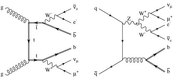
Figure 1: Sample Feynman graphs corresponding to the two resonance histories relevant for $pp\to\mu^{+}\nu_{\mu}e^{-}\bar{\nu}_{e}\,b\,\bar{b}$ production.

we show two corresponding Feynman diagrams for the process $pp\to\mu^{+}\nu_{\mu}e^{-}\bar{\nu}_{e}\,b\,\bar{b}$ .

Internally, according to the POWHEG-BOX-RES conventions Jezo:2015aia , the resonance histories are described by the arrays

  flav_1    = [i,  j,  6, -6,  24, -24, -13,  14,  11, -12,  5, -5],
  flavres_1 = [0,  0,  0,  0,   3,   4,   5,   5,   6,   6,  3,  4],
  flav_2    = [i,  j, 23, 24, -24, -13,  14,  11, -12,   5, -5],
  flavres_2 = [0,  0,  0,  3,   3,   4,   4,   5,   5,   0,  0],

for all relevant choices of initial parton flavours i,j. In flav we store the identities of the initial- and final-state particles, with intermediate resonances, if they exist, labelled according to the Monte Carlo numbering scheme (gluons are labeled by zero in the POWHEG-BOX). In flavres, for each particle, we give the position of the resonance from which it originates. For partons associated with the production subprocess flavres is set to zero.

The resonance structures that differ only by the external parton flavours are collected into resonance groups, so that, in the present case, we have only two resonance groups. We remark that there is no need of a unique correspondence between resonance structures and possible combinations of resonant propagators in individual Feynman diagrams. What is required is that all resonances present in any given Feynman graph are also present in an associated resonance structure, but not vice versa. For example, in the present implementation of the bb4l generator the consistent treatment of single-top topologies like the one in Fig. 2 is guaranteed through resonance histories of $t\bar{t}$ type (flav_1,flavres_1), which involve an additional $\bar{t}\to{\bar{b}}W^{-}$ resonance. This does not lead to any problems, since the corresponding subtraction kinematics, which preserves the mass of the ${\bar{b}}W^{-}$ system, is perfectly adequate also for single-top topologies.

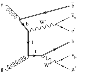
Figure 2: Representative Born diagram for $Wt$ production.

The POWHEG-BOX-RES code automatically recognizes resonance histories that can be collected into the same resonance group. It also includes a subroutine for the automatic generation of an adequate phase-space sampling for each resonance group. In this context, rather than relying upon standard Breit-Wigner sampling, care is taken that also the off-shell regions are adequately populated. This is essential in resonance histories of the kind shown in the right graph of Fig. 1, where the generation of the $W$ virtualities according to their Breit-Wigner shape would well probe the region where an off-shell $Z$ decays into two on-shell $W$’s, but not the regions where an on-shell $Z$ decays into an on-shell $W$ and an off-shell one. It also guarantees that cases like the diagram in Fig. 2 are properly sampled. The interested reader can find more technical details by inspecting the code itself.

4.2 The complex-mass scheme

In our calculation all intermediate massive particles are consistently treated in the complex-mass scheme Denner:1999gp ; Denner:2005fg , where the widths of unstable particles are absorbed into the imaginary part of the corresponding mass parameters,

$$\mu^{2}_{i}=M_{i}^{2}-\mathrm{i}\Gamma_{i}M_{i}\qquad\mbox{for}\ \ i=W,Z,t,H.$$ (7)

This choice implies a complex-valued weak mixing angle,

$$\sin\theta_{W}^{2}=1-\cos\theta_{W}^{2}=1-\frac{\mu_{W}^{2}}{\mu_{Z}^{2}}\,,$$ (8)

and guarantees gauge invariance at NLO Denner:2005fg .

4.3 The decoupling and $\overline{\rm MS}$ schemes

When performing a fixed-order calculation with massive quarks, one can define two consistent renormalization schemes that describe the same physics: the usual $\overline{\rm MS}$ scheme, where all flavours are treated on equal footing, and a mixed scheme Collins:1978wz , that we call decoupling scheme, in which the $n_{\rm lf}$ light flavours are subtracted in the $\overline{\rm MS}$ scheme, while heavy-flavour loops are subtracted at zero momentum. In this scheme, heavy flavours decouple at low energies.

In the calculation of the $\ell^{+}\nu_{\mathchoice{\displaystyle}{\scriptstyle}{\scriptscriptstyle}{\scriptscriptstyle}\ell}\,l^{-}\bar{\nu}_{\mathchoice{\displaystyle}{\scriptstyle}{\scriptscriptstyle}{\scriptscriptstyle}l}\,b\,\bar{b}$ hard scattering cross section we treat the bottom quark as massive and, correspondingly, $n_{\rm lf}$ is equal to four. The renormalization of the virtual contributions is performed in the decoupling scheme with a four-flavour running $\alpha_{\mathchoice{\displaystyle}{\scriptstyle}{\scriptscriptstyle}{\scriptscriptstyle}\rm S}$. For consistency, the evolution of parton distribution functions (PDFs) should be performed with four active flavours, so that, in particular, no bottom-quark density is present and no bottom-quark initiated processes have to be considered. However, given that the process at hand is characterised by typical scales far above the $b$-quark threshold, it is more convenient to convert our results to the ${\overline{\rm MS}}$ scheme in such a way that they can be expressed in terms of the ${\overline{\rm MS}}$ strong coupling constant, running with five active flavours, and also with five-flavour PDFs.

The procedure for such a switch of schemes is well known, and was discussed in Ref. Cacciari:1998it . For $\ell^{+}\nu_{\mathchoice{\displaystyle}{\scriptstyle}{\scriptscriptstyle}{\scriptscriptstyle}\ell}\,l^{-}\bar{\nu}_{\mathchoice{\displaystyle}{\scriptstyle}{\scriptscriptstyle}{\scriptscriptstyle}l}\,b\,\bar{b}$ production, we need to transform the $q\bar{q}$ and $gg$ squared Born amplitudes ${\cal B}_{qq}$ and ${\cal B}_{gg}$, computed in the decoupling scheme, in the following way

$${\cal B}_{qq} \rightarrow \left[1-\frac{4}{3}\,T_{\mathchoice{\displaystyle}{\scriptstyle}{\scriptscriptstyle}{\scriptscriptstyle}\rm F}\,\frac{\alpha_{\mathchoice{\displaystyle}{\scriptstyle}{\scriptscriptstyle}{\scriptscriptstyle}\rm S}}{2\pi}\,\log\left(\frac{\mu_{\mathchoice{\displaystyle}{\scriptstyle}{\scriptscriptstyle}{\scriptscriptstyle}\rm R}^{2}}{m_{b}^{2}}\right)\right]\,{\cal B}_{qq}\,,$$ (9)

$${\cal B}_{gg} \rightarrow \left[1+\frac{4}{3}\,T_{\mathchoice{\displaystyle}{\scriptstyle}{\scriptscriptstyle}{\scriptscriptstyle}\rm F}\,\frac{\alpha_{\mathchoice{\displaystyle}{\scriptstyle}{\scriptscriptstyle}{\scriptscriptstyle}\rm S}}{2\pi}\,\log\left(\frac{\mu_{\mathchoice{\displaystyle}{\scriptstyle}{\scriptscriptstyle}{\scriptscriptstyle}\rm F}^{2}}{\mu_{\mathchoice{\displaystyle}{\scriptstyle}{\scriptscriptstyle}{\scriptscriptstyle}\rm R}^{2}}\right)\right]\,{\cal B}_{gg}\,.$$ (10)

where $\mu_{\mathchoice{\displaystyle}{\scriptstyle}{\scriptscriptstyle}{\scriptscriptstyle}\rm R}$ and $\mu_{\mathchoice{\displaystyle}{\scriptstyle}{\scriptscriptstyle}{\scriptscriptstyle}\rm F}$ are the renormalization and factorization scales, respectively, and $m_{b}$ is the bottom-quark mass. The contribution of the $b$ parton densities, that are present in the five-flavour scheme, should not be included in this context.

4.4 The virtual corrections

The virtual contributions have been generated using the new interface of the POWHEG-BOX with the OpenLoops amplitude generator, as described in Appendix A.3. While OpenLoops guarantees a very fast evaluation of one-loop matrix elements, the overall efficiency of the generator can be significantly improved by minimising the number of phase space points that require the calculation of virtual contributions. As detailed in Appendix A.4, this is is achieved by evaluating the virtual and real-emission contributions with independent statistical accuracies optimised according to the respective relative weights. Moreover, when generating events, a reweighting method can be used in order to restrict virtual evaluations to the small fraction of phase space points that survive the unweighting procedure.

4.5 Interface to the shower

The generator presented in this work shares many common features with the one of Ref. Campbell:2014kua . In particular, in both generators, Les Houches events include resonance information, and an option for a multiple radiation scheme is implemented, denoted as allrad scheme, according to the corresponding powheg.input flag. As explained in Ref. Campbell:2014kua and reviewed in Section 2, when this scheme is activated, the mechanism of radiation generation is modified. Rather than keeping only the hardest radiation arising from all singular regions, the program stores several “hardest radiations”: one that takes place at the production stage, and one for the decay of each resonance that can radiate. All these radiations are assembled into a single Les Houches event. Thus, for example, in events with the $t$ and $\bar{t}$ resonances, one can have up to three radiated partons: one coming from the initial-state particles, one arising from the $b$ in the $t$-decay, and one from the $\bar{b}$ in the $\bar{t}$-decay.

When generating fully showered events, the hardness of the shower must be limited in a way that depends upon the origin of the radiating parton. If the radiating parton is not son of a resonance, the hardness of the shower arising from it must be limited by the hardness of the Les Houches radiation that arises in production. Radiation arising from partons originating from a resonance must have their hardness limited by the hardness of the parton radiated from the resonance in the Les Houches event. This requires a shower interface that goes beyond the Les Houches approach. In Ref. Campbell:2014kua a suitable procedure has been conceived and implemented in Pythia8 Sjostrand:2007gs ; Sjostrand:2014zea . The interested reader can find all details in the Appendix A of  Ref. Campbell:2014kua . In essence, the procedure was to examine the showered event, compute the transverse momentum of Pythia8 radiation in top decays, and veto it if higher than the corresponding POWHEG one. Vetoing is performed by rejecting the showered event, and generating a new Pythia8 shower, initiated by the same Les Houches event. This procedure was iterated until the showered event passes the veto. In the present work, we have adopted this procedure in order to make a more meaningful comparison with the results of Ref. Campbell:2014kua . However, we have also verified that, by using Pythia8 internal mechanism for vetoing radiation from resonance decay, we get results that are fully compatible with our default approach. This aspect and the comparison among the two methods are shown in Appendix B.2.

4.6 Traditional NLO+PS matching

It is possible to run our new generator in a way that is fully equivalent to a standard POWHEG matching algorithm (as implemented in the POWHEG-BOX-V2) ignoring the resonance structure of the processes. This is achieved by including the line nores 1 in the powheg.input file. Such an option is implemented only for the purpose of testing the new formalism with respect to the old one.

It turns out that, in the nores 1 mode, the program has much worse convergence properties, most likely because of the less effective cancellation of infrared singularities mentioned in Section 2. We find, for example, that in runs with equal statistics (with about 15 million calls) the absolute error in the nores 1 case is roughly seven times larger than in the nores 0 (default) case. The generation of events also slows down by a similar factor.

We stress again that, in the limit of small widths, the NLO+PS results obtained in the nores 1 mode are bound to become inconsistent, as discussed in Section 2 and, more extensively, in Ref. Jezo:2015aia .

4.7 Consistency checks

At the level of fixed-order NLO calculations, the traditional machinery of the POWHEG-BOX is well tested and we trust corresponding results to be correct. On the other hand, the NLO subtraction procedure implemented in the POWHEG-BOX-RES code is substantially different and still relatively new. As was done in Ref. Jezo:2015aia for $t$-channel single-top production, also for the $\ell^{+}\nu_{\mathchoice{\displaystyle}{\scriptstyle}{\scriptscriptstyle}{\scriptscriptstyle}\ell}\,l^{-}\bar{\nu}_{\mathchoice{\displaystyle}{\scriptstyle}{\scriptscriptstyle}{\scriptscriptstyle}l}\,b\,\bar{b}$ production presented here, we systematically validated the fixed-order NLO results obtained with the POWHEG-BOX-RES implementation by switching on and off the generation of resonance structures. We found perfect agreement between the two calculations.

Additionally, we performed a detailed comparison against the fixed-order NLO results of Ref. Cascioli:2013wga and found agreement at the permil level. Furthermore, via a numerical scan in the limit of the top width going to zero, $\Gamma_{t}\to 0$, we verified that any $\alpha_{\mathchoice{\displaystyle}{\scriptstyle}{\scriptscriptstyle}{\scriptscriptstyle}\rm S}\log\left(\Gamma_{t}\right)$ enhanced terms in the soft-gluon limit successfully cancel between real and virtual contributions. This last test was performed for various light- and $b$-jet exclusive distributions which are subject to sizable non-resonant/off-shell corrections.

5 Phenomenological setup

In this section we document the input parameters, acceptance cuts and generator settings that have been adopted for the numerical studies presented in Section 6. Moreover we introduce a systematic labelling scheme for the various NLO+PS approximations that are going to be compared.

5.1 Input parameters

Masses and widths are assigned the following values

$$m_{Z} =91.188\;\text{GeV}\,, \Gamma_{Z} =2.441\;\text{GeV}\,,$$ (11)

$$m_{W} =80.419\;\text{GeV}\,, \Gamma_{W} =2.048\;\text{GeV}\,,$$ (12)

$$m_{H} =125\;\text{GeV}\,, \Gamma_{H} =4.03\times 10^{-3}\;\text{GeV}\,,$$ (13)

$$m_{t} =172.5\;\text{GeV}\,, \Gamma_{t} =1.329\;\text{GeV}\,,$$ (14)

$$m_{b} =4.75\;\text{GeV}\,.$$ (15)

The electroweak couplings are derived from the gauge-boson masses and the Fermi constant, ${G_{\mathchoice{\displaystyle}{\scriptstyle}{\scriptscriptstyle}{\scriptscriptstyle}\mu}}=1.16585\times 10^{-5}\leavevmode\nobreak\ \text{GeV}^{-2}$, in the $G_{\mu}$-scheme, via

$$\alpha_{\mathchoice{\displaystyle}{\scriptstyle}{\scriptscriptstyle}{\scriptscriptstyle}\rm EM}=\sqrt{2}\,\frac{G_{\mu}}{\pi}\left|\mu_{\mathchoice{\displaystyle}{\scriptstyle}{\scriptscriptstyle}{\scriptscriptstyle}W}^{2}\left(1-\frac{\mu_{\mathchoice{\displaystyle}{\scriptstyle}{\scriptscriptstyle}{\scriptscriptstyle}W}^{2}}{\mu_{\mathchoice{\displaystyle}{\scriptstyle}{\scriptscriptstyle}{\scriptscriptstyle}Z}^{2}}\right)\right|=\frac{1}{132.50698}\,,$$ (16)

where $\mu_{\mathchoice{\displaystyle}{\scriptstyle}{\scriptscriptstyle}{\scriptscriptstyle}W}$ and $\mu_{\mathchoice{\displaystyle}{\scriptstyle}{\scriptscriptstyle}{\scriptscriptstyle}Z}$ are complex masses given by Eq. (7).

The value of the top-quark width we use is consistently calculated at NLO from all other input parameters by computing the three-body decay widths $\Gamma(t\to f\bar{f}^{\prime}b)$ into any pair of light fermions $f$ and $\bar{f}^{\prime}$ and a massive $b$ quark. To this end, we employ a numerical routine of the MCFM implementation of Ref. Campbell:2012uf .

As parton distributions we have adopted the five-flavour MSTW2008NLO PDFs Martin:2009iq , as implemented in the Ref. Buckley:2014ana , with the corresponding five-flavour strong coupling constant, and for their consistent combination with four-flavour scheme parton-level cross sections the scheme transformation of Section 4.3 was applied. In the evaluation of the matrix elements, only the bottom and the top quarks are massive. All the other quarks are treated as massless. In addition, the Cabibbo-Kobayashi-Maskawa matrix is assumed to be diagonal.

When generating events we adopt the following scale choice:

• For resonance histories with a top pair we use

  $$\mu_{\mathchoice{\displaystyle}{\scriptstyle}{\scriptscriptstyle}{\scriptscriptstyle}\rm R}=\mu_{\mathchoice{\displaystyle}{\scriptstyle}{\scriptscriptstyle}{\scriptscriptstyle}\rm F}=\left[\left(m_{t}^{2}+p_{{T},t}^{2}\right)\left(m_{\bar{t}}^{2}+p_{{T},{\bar{t}}}^{2}\right)\right]^{\frac{1}{4}}\;,$$ (17)

  where the (anti)top masses and transverse momenta are defined in the underlying Born phase space in terms of final state (off-shell) decay products.

• For resonance histories with an intermediate $Z$ we use

  $$\mu_{\mathchoice{\displaystyle}{\scriptstyle}{\scriptscriptstyle}{\scriptscriptstyle}\rm R}=\mu_{\mathchoice{\displaystyle}{\scriptstyle}{\scriptscriptstyle}{\scriptscriptstyle}\rm F}=\frac{\sqrt{p_{Z}^{2}}}{2}\;,$$ (18)

  where $p_{Z}=p_{\ell^{+}}+p_{\nu_{\ell}}+p_{l^{-}}+p_{\bar{\nu}_{l}}$.

In addition, we set the value of the POWHEG-BOX parameter hdamp to the mass of the top quark. This setting yields a transverse-momentum distribution of the top pair that is more sensitive to scale variations and more consistent with data at large transverse momenta. It only affects initial-state radiation. For a detailed description of this parameter, we refer the reader to Ref. Alioli:2008tz .

5.2 Pythia8 settings

We interface our POWHEG generator to Pythia8.1, as illustrated in Appendix A of Ref. Campbell:2014kua , and so we perform the following Pythia8 calls:

    pythia.readString("SpaceShower:pTmaxMatch = 1");
    pythia.readString("TimeShower:pTmaxMatch = 1");
    pythia.readString("PartonLevel:MPI = off");
    pythia.readString("SpaceShower:QEDshowerByQ = off");
    pythia.readString("SpaceShower:QEDshowerByL = off");
    pythia.readString("TimeShower:QEDshowerByQ = off");
    pythia.readString("TimeShower:QEDshowerByL = off");

The first two calls are required when interfacing Pythia8 to NLO+PS generators. The third call switches off multi-parton interactions and it is only invoked for performance reasons: in fact, the shower of the events is faster when multi-parton interactions are not simulated. The remaining calls switch off the electromagnetic radiation in Pythia8. This makes it easier to reconstruct the $W$ boson momentum, since we do not need to dress the charged lepton, from vector boson decay, with electromagnetic radiation. These settings are appropriate in the present context since we do not make any comparison with data.

Pythia8 provides by default matrix-element corrections Norrbin:2000uu . In our case, they are relevant for radiation in the top decays, which are corrected using $t\to Wbg$ tree level matrix elements. These corrections are also applied in subsequent emissions in order to better model radiation from heavy flavours in general. If not explicitly stated otherwise, we include the following setup calls

    pythia.readString("TimeShower:MEcorrections = on");
    pythia.readString("TimeShower:MEafterFirst = on");

These corrections never modify the Les Houches event weight. They only affect the radiation generated by the shower. Thus, leaving these flags on does not lead to over-counting. If the second flag is off, matrix-element corrections are applied only to the first shower emission. If it is on, they are also applied to subsequent radiation. In fact, even if these corrections cannot fully account for the structure of the matrix elements, they at least better account for mass effects arising in radiation from the off-shell top quarks and from the massive final-state $b$’s.

In our analysis, we keep $B$ hadrons stable, performing the corresponding Pythia8 setup calls. Aside from these, all remaining settings are left to the defaults of Pythia8.1.

5.3 Generators and labels

In Section 6 we compare three different generators that implement an increasingly precise treatment of $t\bar{t}$ production and decay:

• the hvq generator of Ref. Frixione:2007nw ;

• the ttb_NLO_dec generator of Ref. Campbell:2014kua ;

• the new bb4l generator, which we consider as our best prediction.

label	$t\bar{t}$	$t\bar{t}\,\otimes\,$decay	$b\bar{b}4\ell$
generator	hvq Frixione:2007nw	ttb_NLO_dec Campbell:2014kua	bb4l
framework	POWHEG-BOX	POWHEG-BOX-V2	POWHEG-BOX-RES
NLO matrix elements	$t\bar{t}$	$t(\to\ell^{+}\nu_{\mathchoice{\displaystyle}{\scriptstyle}{\scriptscriptstyle}{\scriptscriptstyle}\ell}b)\,\bar{t}(\to l^{-}\bar{\nu}_{\mathchoice{\displaystyle}{\scriptstyle}{\scriptscriptstyle}{\scriptscriptstyle}l}\bar{b})$	$\ell^{+}\nu_{\mathchoice{\displaystyle}{\scriptstyle}{\scriptscriptstyle}{\scriptscriptstyle}\ell}\,l^{-}\bar{\nu}_{\mathchoice{\displaystyle}{\scriptstyle}{\scriptscriptstyle}{\scriptscriptstyle}l}\,b\,\bar{b}$
decay accuracy	LO+PS	NLO+PS	NLO+PS
NLO radiation	single	multiple	multiple
spin correlations	approx.	exact	exact
off-shell $t\bar{t}$ effects	BW smearing	LO $b\bar{b}4\ell$ reweighting	exact
$Wt$ & non-resonant effects	no	LO $b\bar{b}4\ell$ reweighting	exact
$b$-quark massive	yes	yes	yes

Table 1: Labels and characteristic features of the three generators considered in this paper.

The main physics features of the various generators and the labels that will be used to identify the corresponding predictions are listed in Table 1. All generators are run with their default settings and are interfaced to Pythia8.1. The bb4l generator implements the scale choice of Eqs. (17)–(18), while in ttb_NLO_dec and hvq a scale corresponding to Eq. (17) is used.

In order to quantify the impact of various aspects of the resonance-aware approach, in Section 6 we will compare various settings of the bb4l generator where some resonance-aware improvements are turned on and off or are replaced by certain approximations. Specifically, the following settings will be considered:

• the resonance-aware formalism is switched on with default settings;

• the resonance-aware formalism is switched off, which corresponds to using the traditional POWHEG approach;

• the resonance-aware formalism is switched off, but a resonance assignment is guessed based on the kinematic structure of the events, according to the method described in Appendix B.1;

• the resonance-aware formalism is switched on, but, instead of applying the multiple-radiation scheme of Eq. (6), only a single radiation is generated with POWHEG according to Eq. (1);

• same as (d), but the resonance information is stripped off in the POWHEG Les Houches event file before passing it to the showering program.

The various bb4l settings and corresponding labels are summarised in Table 2.

	$b\bar{b}4\ell$ setting	resonance-aware	radiation in	flags in the
	label	matching	production and decay	powheg.input
(a)	res-default	yes	multiple	1, 0, 0, 0
(b)	res-off	no	single	0, 0, 0, 1
(c)	res-guess	no (kinematic guess)	single	0, 0, 1, 1
(d)	res-singlerad	yes	single	0, 0, 0, 0
(e)	res-strip	yes (stripped off)	single	0, 1, 0, 0

Table 2: Labels for the various $b\bar{b}4\ell$ predictions that are considered and compared in this paper. In the last column we list the values of the POWHEG-BOX flags allrad, stripres, guessres, nores, to be specified in the powheg.input file.

5.4 Physics objects

In the subsequent sections we study various observables defined in terms of the following physics objects.

1. We denote as $B$ and $\bar{B}$ hadron the hardest $b$-flavoured and $\bar{b}$-flavoured hadron in the event.

2. Final-state hadrons are recombined into jets using the FastJet implementation Cacciari:2011ma of the anti-$k_{\mathchoice{\displaystyle}{\scriptstyle}{\scriptscriptstyle}{\scriptscriptstyle}T}$ jet algorithm Cacciari:2008gp with $R=0.5$.

3. We denote as $b$-jet (${j_{\rm\mathchoice{\displaystyle}{\scriptstyle}{\scriptscriptstyle}{\scriptscriptstyle}B}}$) and anti-$b$-jet ($j_{\rm\mathchoice{\displaystyle}{\scriptstyle}{\scriptscriptstyle}{\scriptscriptstyle}{\bar{B}}}$) the jet that contains the hardest $B$ and $\bar{B}$ hadron, respectively. When examining results obtained with the hadronization switched off, jets are $b$-tagged based on $b$ quarks rather than $B$ hadrons.

4. Leptons, neutrinos and missing transverse energy are identical to their corresponding objects at matrix-element level, since we switched off QED radiation and hadron decays in Pythia8.

5. Reconstructed $W^{+}$ and $W^{-}$ bosons are identified with the corresponding off-shell lepton-neutrino pairs in the hard matrix elements.

6. Reconstructed top and anti-top quarks are defined as off-shell $W^{+}{j_{\rm\mathchoice{\displaystyle}{\scriptstyle}{\scriptscriptstyle}{\scriptscriptstyle}B}}$ and $W^{-}j_{\rm\mathchoice{\displaystyle}{\scriptstyle}{\scriptscriptstyle}{\scriptscriptstyle}{\bar{B}}}$ pairs, respectively, i.e. $b$-jets and $W$-bosons are matched based on charge and $b$-flavour information at Monte-Carlo truth level. The same approach is used for $\ell^{+}{j_{\rm\mathchoice{\displaystyle}{\scriptstyle}{\scriptscriptstyle}{\scriptscriptstyle}B}}$ and $\l^{-}j_{\rm\mathchoice{\displaystyle}{\scriptstyle}{\scriptscriptstyle}{\scriptscriptstyle}{\bar{B}}}$ pairs.

Unless stated otherwise, in kinematic distributions we always perform an average over the $t$ and $\bar{t}$ case (thus also on lepton–antilepton, $b$–anti-$b$, etc.).

The top-pair observables in Sections 6.2–6.3 are computed by requiring the presence of a $b$ and a $\bar{b}$ jet with

$$p_{\mathchoice{\displaystyle}{\scriptstyle}{\scriptscriptstyle}{\scriptscriptstyle}T}^{j}>30\leavevmode\nobreak\ \text{GeV},\qquad\qquad|\eta^{j}|<2.5\,,$$ (19)

and applying the following leptonic cuts,

$$p_{\mathchoice{\displaystyle}{\scriptstyle}{\scriptscriptstyle}{\scriptscriptstyle}T}^{l}>20\leavevmode\nobreak\ \text{GeV},\qquad|\eta^{l}|<2.5\,,\qquad p_{\mathchoice{\displaystyle}{\scriptstyle}{\scriptscriptstyle}{\scriptscriptstyle}T}^{\mathchoice{\displaystyle}{\scriptstyle}{\scriptscriptstyle}{\scriptscriptstyle}\mathrm{miss}}>20\leavevmode\nobreak\ \text{GeV},$$ (20)

where $l=\ell^{+},l^{-}$ and $p_{\mathchoice{\displaystyle}{\scriptstyle}{\scriptscriptstyle}{\scriptscriptstyle}T}^{\mathchoice{\displaystyle}{\scriptstyle}{\scriptscriptstyle}{\scriptscriptstyle}\mathrm{miss}}$ is obtained from the vector sum of the transverse momentum of the neutrinos in the final state.

6 Top-pair dominated observables

Here we present numerical predictions for $pp\to e^{+}\nu_{e}\mu^{-}\bar{\nu}_{\mu}b\,\bar{b}+X$ at $\sqrt{s}=$8 TeV. In particular, we study various observables that are sensitive to the shape of top resonances.

6.1 Comparison with traditional NLO+PS matching

In the following, we compare nominal bb4l predictions, generated with default settings, with results obtained by switching off the resonance-aware formalism (i.e. setting the flag nores to 1). In this way we get results that are fully equivalent to a POWHEG-BOX-V2 (or “traditional”) implementation. For this comparison we do not impose any cuts, i.e. we perform a fully inclusive analysis that involves, besides $t\bar{t}$ production, also significant contributions from $Wt$ single-top production.

Events generated with the traditional implementation do not contain any information whatsoever about their resonance structures. We label the curves obtained by showering these events as res-off. Because the resonance information is not available, the shower generator will not preserve the virtualities of the resonances. In order to further explore the usability of the res-off results, we also consider the possibility of reconstructing the resonance information of the Les Houches event on the basis of its kinematic proximity to one of the possible resonant configurations. Specifically, we perform an educated guess of the resonance structure of the event, assigning it to a $t{\bar{t}}$ or to a $Z$ resonance configuration (see Section 4.1), and assigning the radiation either to the initial state or to the outgoing $b$’s. The curves obtained this way are labelled as res-guess and the procedure for reconstructing the resonance information from the event kinematics is detailed in Appendix B.1.

We first consider, in Fig. 3,

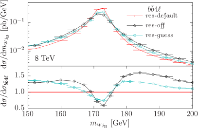
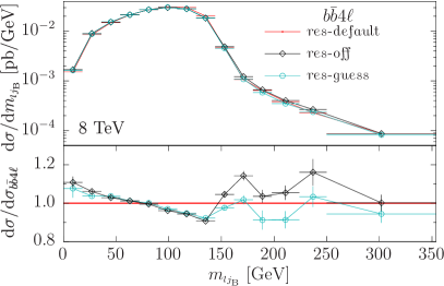
Figure 3: NLO+PS predictions for the invariant mass of the $W{j_{\rm\mathchoice{\displaystyle}{\scriptstyle}{\scriptscriptstyle}{\scriptscriptstyle}B}}$ (left) and of the $l{j_{\rm\mathchoice{\displaystyle}{\scriptstyle}{\scriptscriptstyle}{\scriptscriptstyle}B}}$ (right) systems obtained with the new bb4l generator. We compare our default resonance-aware predictions (res-default) against the “traditional”, i.e. resonance-unaware, implementation (res-off) and a prediction where the event-by-event resonance information is obtained from a guess based on kinematics. In the ratio plot we illustrate relative deviations with respect to res-default.

the invariant mass of the $W{j_{\rm\mathchoice{\displaystyle}{\scriptstyle}{\scriptscriptstyle}{\scriptscriptstyle}B}}$ and of the $l{j_{\rm\mathchoice{\displaystyle}{\scriptstyle}{\scriptscriptstyle}{\scriptscriptstyle}B}}$ systems. In the res-off case, we observe that the reconstructed mass peak has a wider shape. This is expected, since neither the POWHEG-BOX nor the shower program preserve the virtuality of the top resonances. In the res-guess case the width of the peak is diminished, although not quite at the level of the resonance-aware prediction, labelled as res-default. We also observe a mild shift in the peak in the res-guess case, which improves the agreement with the res-default result. The distribution in the mass of the lepton-${j_{\rm\mathchoice{\displaystyle}{\scriptstyle}{\scriptscriptstyle}{\scriptscriptstyle}B}}$ system also shows marked differences in shape in the region that is most relevant for a top-mass determination, with more pronounced differences in the res-off case.

The above findings suggest that the width of the peak is determined both by the shower generator being aware of the resonances in the Les Houches event, and by the hardest radiation generation being performed in a way that is consistent with the resonance structure. In order to assess the effects that originate solely from resonance-aware matching and showering in a more accurate way, in Fig. 4

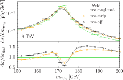
Figure 4: Invariant mass of the $W{j_{\rm\mathchoice{\displaystyle}{\scriptstyle}{\scriptscriptstyle}{\scriptscriptstyle}B}}$ system obtained with the bb4l generator. We compare our resonance-aware predictions without employing the multiple radiation scheme (res-singlerad) against the “traditional”, i.e. resonance-unaware, implementation (res-off) and a prediction where any resonance information is stripped off the Les Houches event file (res-strip). In the ratio plot we illustrate relative deviations with respect to res-singlerad.

we disable the multiple radiation scheme of Eq. (6) (by setting allrad 0) and compare the resulting resonance-aware predictions (res-singlerad) against the cases where resonance information is removed from the Les Houches event before showering (res-strip) or the case where the resonance-aware system is completely switched off (res-off). We find that the res-strip result lies between the res-singlerad and the res-off ones, somewhat closer to the latter, and the differences between the various predictions are considerable. Therefore, we conclude that the observed widening of the peak in Figures 3–4 can be attributed to both shortcomings of a resonance unaware parton shower matching: the parton shower reshuffling not preserving the resonance masses, and the uncontrolled effects of resonances at the level of the first emission in the traditional POWHEG approach.

In Fig. 5 we display

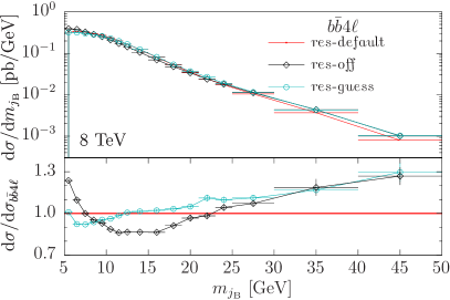
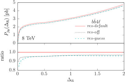
Figure 5: Mass (left) and profile (right) of the $b$-jet ${j_{\rm\mathchoice{\displaystyle}{\scriptstyle}{\scriptscriptstyle}{\scriptscriptstyle}B}}$. Absolute predictions and ratios as in Fig. 3.

the ${j_{\rm\mathchoice{\displaystyle}{\scriptstyle}{\scriptscriptstyle}{\scriptscriptstyle}B}}$ mass and profile, defined as

$$P_{{j_{\rm\mathchoice{\displaystyle}{\scriptstyle}{\scriptscriptstyle}{\scriptscriptstyle}B}}}(\Delta_{\mathchoice{\displaystyle}{\scriptstyle}{\scriptscriptstyle}{\scriptscriptstyle}\mathrm{R}})=\int{\mathrm{d}}\sigma\;\frac{\sum_{j}p_{\mathchoice{\displaystyle}{\scriptstyle}{\scriptscriptstyle}{\scriptscriptstyle}T}^{\mathchoice{\displaystyle}{\scriptstyle}{\scriptscriptstyle}{\scriptscriptstyle}j}\,\theta\!\left(\Delta_{\mathchoice{\displaystyle}{\scriptstyle}{\scriptscriptstyle}{\scriptscriptstyle}\mathrm{R}}-\Delta_{\mathchoice{\displaystyle}{\scriptstyle}{\scriptscriptstyle}{\scriptscriptstyle}\mathrm{R}}^{(j,{j_{\rm\mathchoice{\displaystyle}{\scriptstyle}{\scriptscriptstyle}{\scriptscriptstyle}B}})}\right)}{p_{\mathchoice{\displaystyle}{\scriptstyle}{\scriptscriptstyle}{\scriptscriptstyle}T}^{j_{\rm\mathchoice{\displaystyle}{\scriptstyle}{\scriptscriptstyle}{\scriptscriptstyle}B}}}\,.$$ (21)

This observable corresponds to the cross section weighted by the fraction of the total hadronic transverse momentum of the particles contained in a given cone around the jet axis, with respect to the transverse momentum of the $b$-jet. Again we observe marked differences among the res-default and the res-off results, and, to a lesser extent, between the res-default and res-guess ones. Both plots suggest that in the res-off case there is less activity around the $B$ hadron, leading to smaller jet masses and to a slightly steeper jet profile. The particularly pronounced shape distortion of the ${j_{\rm\mathchoice{\displaystyle}{\scriptstyle}{\scriptscriptstyle}{\scriptscriptstyle}B}}$ mass plot near 10 GeV in the res-guess case can be tentatively attributed to the transition from the region where radiation (generated with the traditional method) does not change the mass of the resonance by an amount comparable or larger than its width, to the region where it does, so that we see the difference between the res-guess and res-default results grow with larger jet masses.

In Fig. 6

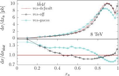
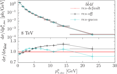
Figure 6: $B$ fragmentation function and $B$-hadron transverse momentum in the top decay frame. Absolute predictions and ratios as in Fig. 3.

we compare the $B$ fragmentation function and the $B$-hadron transverse momentum computed in the reconstructed top-decay rest frame. The $x_{\mathchoice{\displaystyle}{\scriptstyle}{\scriptscriptstyle}{\scriptscriptstyle}\rm B}$ variable is defined as the $B$ energy in the reconstructed top rest frame normalized to the maximum value that it can attain at the given top virtuality, while $p^{\rm\mathchoice{\displaystyle}{\scriptstyle}{\scriptscriptstyle}{\scriptscriptstyle}B}_{\mathchoice{\displaystyle}{\scriptstyle}{\scriptscriptstyle}{\scriptscriptstyle}\rm T,dec}$ is the transverse momentum of the $B$ relative to the recoiling $W$ in the same frame. We find marked differences also for these distributions. While in the case of the $p^{\rm\mathchoice{\displaystyle}{\scriptstyle}{\scriptscriptstyle}{\scriptscriptstyle}B}_{\mathchoice{\displaystyle}{\scriptstyle}{\scriptscriptstyle}{\scriptscriptstyle}\rm T,dec}$ variable we see a reasonable consistency between the res-guess and res-default results, the agreement deteriorates in the case of the fragmentation function.

We conclude that the consistent treatment of resonances implemented in the bb4l generator yields a narrower peak for the reconstructed top distribution with respect to a traditional (resonance-blind) NLO+PS matching approach. Furthermore, a large part of the difference is not related to the lack of resonance information at the level of the shower generator, and thus cannot be reduced by using a more sophisticated interface to the shower based on a resonance-guessing approach of kinematic nature.

6.2 Comparison with the ttb_NLO_dec generator

In this section we compare the bb4l generator against the ttb_NLO_dec generator of Ref. Campbell:2014kua . The standard $t\bar{t}$ cuts of Eqs. (19)–(20) are applied throughout. We examined a large set of distributions, but here we only display the most relevant ones, and those that show the largest discrepancies.

We begin by showing in Fig. 7

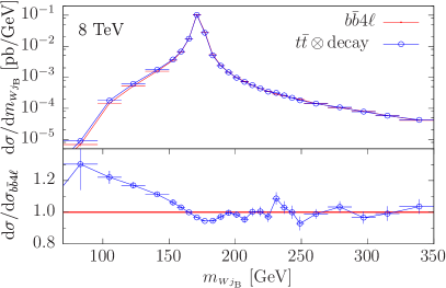
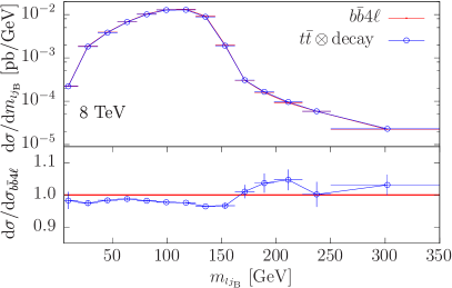
Figure 7: Invariant mass of the $W{j_{\rm\mathchoice{\displaystyle}{\scriptstyle}{\scriptscriptstyle}{\scriptscriptstyle}B}}$ (left) and of the $l{j_{\rm\mathchoice{\displaystyle}{\scriptstyle}{\scriptscriptstyle}{\scriptscriptstyle}B}}$ (right) systems. Comparison of NLO+PS predictions obtained with the bb4l ($b\bar{b}4\ell$) and the ttb_NLO_dec ($t\bar{t}\,\otimes\,$decay) generators. In the ratio plot we illustrate relative deviations with respect to the $b\bar{b}4\ell$ prediction.

the invariant mass distribution of the $W{j_{\rm\mathchoice{\displaystyle}{\scriptstyle}{\scriptscriptstyle}{\scriptscriptstyle}B}}$ and $l{j_{\rm\mathchoice{\displaystyle}{\scriptstyle}{\scriptscriptstyle}{\scriptscriptstyle}B}}$ systems. We observe remarkable agreement between the bb4l and ttb_NLO_dec generators, especially in the description of the reconstructed top peak and of the shoulder in the lepton-${j_{\rm\mathchoice{\displaystyle}{\scriptstyle}{\scriptscriptstyle}{\scriptscriptstyle}B}}$ invariant mass. This agreement is quite reassuring. In fact, in the ttb_NLO_dec generator, the separation of radiation in production and resonance decay is unambiguous, while in bb4l it is based on a probabilistic approach according to a kinematic proximity criterion. Thus, in the light of Fig. 7, the former generator supports the method of separation of resonance histories adopted by the latter. On the other hand, off-shell and non-resonant effects are implemented in the ttb_NLO_dec generator in LO approximation, by reweighting the on-shell result. Thus the bb4l results support the validity of this approximation in the ttb_NLO_dec implementation. As an indicative estimate of the potential implications for precision $m_{t}$ determination, we have determined that in a window of $\pm 30$ GeV around the peak of the $W{j_{\rm\mathchoice{\displaystyle}{\scriptstyle}{\scriptscriptstyle}{\scriptscriptstyle}B}}$ distributions, the average $W{j_{\rm\mathchoice{\displaystyle}{\scriptstyle}{\scriptscriptstyle}{\scriptscriptstyle}B}}$ mass computed with the ttb_NLO_dec generator is roughly 0.1 GeV smaller than the one from bb4l.

The NLO distribution in the mass of the reconstructed top was also examined in Ref. Campbell:2014kua (sec. 3.2, Fig. 3). There, the ttb_NLO_dec fixed-order NLO result was compared to the fixed-order NLO result of Ref. Denner:2012yc , and the former was found to be enhanced by about 10% in a region of roughly 1 GeV around the peak. This comparison was carried out with massless $b$ quarks, since mass effects were not available in Ref. Denner:2012yc . We computed the same distribution and carried out the same NLO comparison, using however the bb4l generator instead of the result of Ref. Denner:2012yc and taking into account $b$-mass effects. Again, we find the same enhancement in the ttb_NLO_dec NLO result. However, in the fully showered result we see instead a small suppression of the peak in the ttb_NLO_dec relative to the bb4l generator, suggesting that the NLO difference tends to be washed out by showering effects.

We examined several distributions involving $b$-jets (here again we average over the $b$- and $\bar{b}$-jet contributions). We found no appreciable difference for the $b$-jet transverse momentum, while we did find significant differences in the jet mass and the jet profile, displayed in Fig. 8.

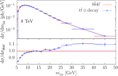
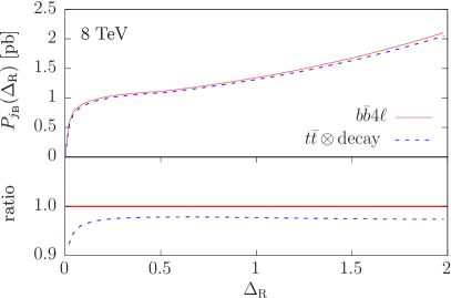
Figure 8: Mass (left) and profile (right) of the ${j_{\rm\mathchoice{\displaystyle}{\scriptstyle}{\scriptscriptstyle}{\scriptscriptstyle}B}}$. Absolute predictions and ratios as in Fig. 7.

Both plots indicate that the bb4l generator yields slightly wider $b$-jets as compared to the ttb_NLO_dec one.

In Fig. 9 we plot the $B$ fragmentation function and the $p^{\rm\mathchoice{\displaystyle}{\scriptstyle}{\scriptscriptstyle}{\scriptscriptstyle}B}_{\mathchoice{\displaystyle}{\scriptstyle}{\scriptscriptstyle}{\scriptscriptstyle}\rm T,dec}$ observables.

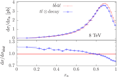
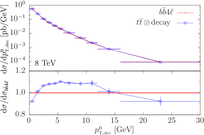
Figure 9: The $B$ fragmentation function and transverse-momentum distribution of the $p^{\rm\mathchoice{\displaystyle}{\scriptstyle}{\scriptscriptstyle}{\scriptscriptstyle}B}_{\mathchoice{\displaystyle}{\scriptstyle}{\scriptscriptstyle}{\scriptscriptstyle}\rm T,dec}$ observable. Absolute predictions and ratios as in Fig. 7.

We find that the fragmentation function is slightly harder, and the $p^{\rm\mathchoice{\displaystyle}{\scriptstyle}{\scriptscriptstyle}{\scriptscriptstyle}B}_{\mathchoice{\displaystyle}{\scriptstyle}{\scriptscriptstyle}{\scriptscriptstyle}\rm T,dec}$ distribution is slightly softer in the bb4l case. Again, this is consistent with the observation of slightly reduced radiation from $b$’s in the bb4l case. We have verified that this feature persists also when hadronization is switched off in Pythia8.

Although the differences in the $b$-jet structure are quite significant, they are not sufficient to induce an observable shift in the reconstructed mass peak. This could only happen if the difference in the jet profile caused a consistent difference in the jet energy, due to energy loss outside the jet-cone. This does not seem to be the case since the jet profiles become similar in the two generators already for $\Delta_{\rm R}<0.5$.

6.3 Comparison with the hvq generator

In this section we compare the bb4l generator against the hvq generator of Ref. Frixione:2007vw , which is based on on-shell NLO matrix elements for $t\bar{t}$ production. Again the standard $t\bar{t}$ cuts of Eqs. (19)–(20) are applied throughout. The $W{j_{\rm\mathchoice{\displaystyle}{\scriptstyle}{\scriptscriptstyle}{\scriptscriptstyle}B}}$ and $l{j_{\rm\mathchoice{\displaystyle}{\scriptstyle}{\scriptscriptstyle}{\scriptscriptstyle}B}}$ mass distributions, shown in Fig. 10,

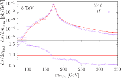
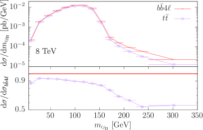
Figure 10: Invariant mass of the $W{j_{\rm\mathchoice{\displaystyle}{\scriptstyle}{\scriptscriptstyle}{\scriptscriptstyle}B}}$ (left) and of the $l{j_{\rm\mathchoice{\displaystyle}{\scriptstyle}{\scriptscriptstyle}{\scriptscriptstyle}B}}$ (right) systems. Comparison of NLO+PS predictions obtained with the bb4l ($b\bar{b}4\ell$) and the hvq ($t\bar{t}$) generators. In the ratio plot we illustrate relative deviations with respect to the $b\bar{b}4\ell$ prediction.

show reasonably good agreement between the two generators as far as the shape of the $W{j_{\rm\mathchoice{\displaystyle}{\scriptstyle}{\scriptscriptstyle}{\scriptscriptstyle}B}}$ peak and of the $l{j_{\rm\mathchoice{\displaystyle}{\scriptstyle}{\scriptscriptstyle}{\scriptscriptstyle}B}}$ shoulder are concerned. However, for large top virtualities, i.e. in the tails of both distributions, sizable differences can be appreciated. As we will see below, such differences originate from the fact that, in this region, the bb4l generator tends to radiate considerably less, which results in narrower b-jets as compared to the hvq generator. We note that the observed deviations with respect to the hvq generator are more drastic than the ones observed in section 6.2 for the ttb_NLO_dec generator. The $m_{W{j_{\rm\mathchoice{\displaystyle}{\scriptstyle}{\scriptscriptstyle}{\scriptscriptstyle}B}}}$ distribution on the left of Fig. 10 additionally suggests a non-negligible shift in the reconstructed top mass between the two generators. In fact, we determined that in a window of $\pm 30$ GeV around the peak of the $m_{W{j_{\rm\mathchoice{\displaystyle}{\scriptstyle}{\scriptscriptstyle}{\scriptscriptstyle}B}}}$ distributions, the average $W{j_{\rm\mathchoice{\displaystyle}{\scriptstyle}{\scriptscriptstyle}{\scriptscriptstyle}B}}$ mass computed with the hvq generator is roughly 0.5 GeV smaller than with the bb4l one.

In Fig. 11

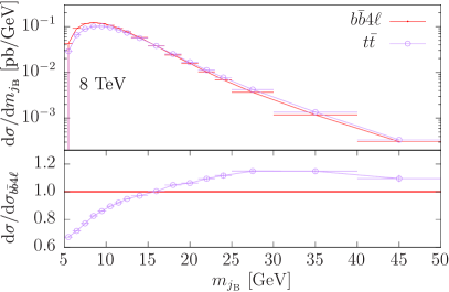
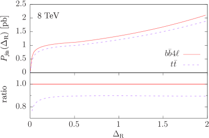
Figure 11: Mass (left) and profile (right) of ${j_{\rm\mathchoice{\displaystyle}{\scriptstyle}{\scriptscriptstyle}{\scriptscriptstyle}B}}$. Absolute predictions and ratios as in Fig. 10.

we show distributions in the $b$-jet mass and profile, as defined in Eq. (21). Both plots indicate significantly narrower $b$-jets in the predictions obtained with the bb4l generator. Similarly, as shown in Fig. 12,

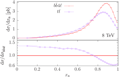
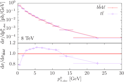
Figure 12: The $B$ fragmentation function and $p^{\rm\mathchoice{\displaystyle}{\scriptstyle}{\scriptscriptstyle}{\scriptscriptstyle}B}_{\mathchoice{\displaystyle}{\scriptstyle}{\scriptscriptstyle}{\scriptscriptstyle}\rm T,dec}$ distribution. Absolute predictions and ratios as in Fig. 10.

the bb4l generator yields a harder $B$ fragmentation function and a softer $p^{\rm\mathchoice{\displaystyle}{\scriptstyle}{\scriptscriptstyle}{\scriptscriptstyle}B}_{\mathchoice{\displaystyle}{\scriptstyle}{\scriptscriptstyle}{\scriptscriptstyle}\rm T,dec}$ distribution. The pattern we observe for the structure of $b$-jets is consistent with the fact that the bb4l generator has a reduced radiation in $b$-jets with respect to Pythia8. In the hvq generator, radiation from the $b$’s is handled exclusively by Pythia8, while, in the bb4l generator, the hardest radiation from the $b$ is handled by POWHEG. It should be stressed, however, that the $B$ fragmentation function has a considerable sensitivity to the hadronization parameters. It would therefore be desirable to tune these parameters to $B$ production data in $e^{+}e^{-}$ annihilation, within the POWHEG framework, in order to perform a meaningful comparison.

In Fig. 13 we show a summary of the shape of the reconstructed top peak comparing each of the available POWHEG generators for $t\bar{t}$ production: bb4l, ttb_NLO_dec and hvq. We notice a fair consistency between the bb4l generator and the ttb_NLO_dec one, while larger deviations are observed comparing against hvq.

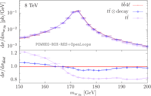
Figure 13: The $W{j_{\rm\mathchoice{\displaystyle}{\scriptstyle}{\scriptscriptstyle}{\scriptscriptstyle}B}}$ mass distribution near the top peak for the three generators bb4l ($b\bar{b}4\ell$), ttb_NLO_dec ($t\bar{t}\,\otimes\,$decay) and hvq ($t\bar{t}$). In the ratio plot we illustrate relative deviations with respect to the $b\bar{b}4\ell$ prediction.

7 Jet vetoes and single-top enriched observables

In this section we investigate the behaviour of the ${\tt bb4l}$ generator in the presence of $b$-jet and light-jet vetoes. Such kinematic restrictions are widely used in order to reduce top backgrounds in $H\to W^{+}W^{-}$ studies and in many other analyses that involve charged leptons and missing energy. Also, jet vetoes play an essential role for experimental studies of $Wt$ single-top production Chatrchyan:2014tua ; Aad:2015eto . In particular, the separation of $Wt$ and $t\bar{t}$ production typically relies upon the requirement that one large transverse-momentum $b$-jet is missing in the first process.

From the theoretical point of view, the separation of $Wt$ and $t\bar{t}$ production is not a clear cut one, since the two processes interfere. As pointed out in the introduction, in the ${\tt bb4l}$ generator this problem is solved by providing a unified description of $t\bar{t}$ and $Wt$ production and decay, where also interference effects are included at NLO. Thus jet vetoes are expected to enrich the relative single-top content of ${\tt bb4l}$ samples, resulting in significant differences with respect to other generators that do not include $Wt$ contributions and interferences at NLO. The bb4l generator is particularly well-suited for the study of jet vetoes also because it includes $b$-mass effects, NLO radiation in top-production and -decay subprocesses, as well as resummation of multiple QCD emissions and hadronization effects as implemented in the parton shower.

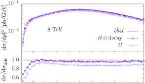
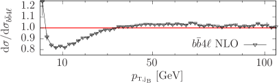
Figure 14: Distribution in the $b$-jet transverse momentum: comparison of NLO+PS predictions obtained with the three generators bb4l ($b\bar{b}4\ell$), ttb_NLO_dec ($t\bar{t}\,\otimes\,$decay) and hvq($t\bar{t}$). The middle frame illustrates relative NLO+PS deviations with respect to the $b\bar{b}4\ell$ prediction, while the lower frame compares $b\bar{b}4\ell$ versus corresponding fixed-order NLO results.

A first picture of the $b$-jet activity in the three generators, bb4l, ttb_NLO_dec and hvq (labelled according to Table 1 as $b\bar{b}4\ell$, $t\bar{t}\,\otimes\,$decay and $t\bar{t}$ respectively), is provided by Fig. 14, where we compare NLO+PS distributions in the transverse momentum of the $b$-jet. More precisely, the plotted observable corresponds to the sum of the $b$- and $\bar{b}$-jet spectra and was computed in absence of any acceptance cut. Thus it involves potentially enhanced contributions from single-top topologies, which can lead to significant deviations between the $t\bar{t}$ prediction and the ones that implement off-shell $\ell^{+}\nu_{\mathchoice{\displaystyle}{\scriptstyle}{\scriptscriptstyle}{\scriptscriptstyle}\ell}\,l^{-}\bar{\nu}_{\mathchoice{\displaystyle}{\scriptstyle}{\scriptscriptstyle}{\scriptscriptstyle}l}\,b\,\bar{b}$ matrix elements. At large transverse momentum, the various predictions have rather similar shape, but the $t\bar{t}$ result features a clear deficit of about 10% with respect the $b\bar{b}4\ell$ and $t\bar{t}\,\otimes\,$decay ones. This can be attributed to the missing single-top contributions in the hvq generator. At high $p_{\mathchoice{\displaystyle}{\scriptstyle}{\scriptscriptstyle}{\scriptscriptstyle}T}$, thanks to the implementation of $Wt$ contributions via exact Born matrix elements for $pp\,\to\,\ell^{+}\nu_{\mathchoice{\displaystyle}{\scriptstyle}{\scriptscriptstyle}{\scriptscriptstyle}\ell}\,l^{-}\bar{\nu}_{\mathchoice{\displaystyle}{\scriptstyle}{\scriptscriptstyle}{\scriptscriptstyle}l}\,b\,\bar{b}$, the $t\bar{t}\,\otimes\,$decay prediction is found to be in good agreement with the $b\bar{b}4\ell$ one. At small transverse momenta, the relative weight of $Wt$ production becomes more important, and the deficit of the $t\bar{t}$ prediction grows rather quickly, reaching up to 50% for very small transverse momenta. The $t\bar{t}\,\otimes\,$decay and $b\bar{b}4\ell$ predictions remain in good agreement down to $p_{{\rm T},{j_{\rm\mathchoice{\displaystyle}{\scriptstyle}{\scriptscriptstyle}{\scriptscriptstyle}B}}}\simeq 10$ GeV, but at smaller transverse momenta the $t\bar{t}\,\otimes\,$decay one develops a deficit that grows up to about 25%. This can be attributed, at least in part, to the increased importance of $Wt$ channels combined with the fact that these channels are not supplemented by an appropriate NLO correction in the $t\bar{t}\,\otimes\,$decay predictions. We also note that the discrepancy at hand can be interpreted as a kinematic shift of a few GeV only, while the enhancement of the resulting correction can be attributed to the pronounced steepness of the absolute $p_{{\rm T},{j_{\rm\mathchoice{\displaystyle}{\scriptstyle}{\scriptscriptstyle}{\scriptscriptstyle}B}}}$ distribution in the soft region. Its sign is consistent with the fact that radiation arising from $\ell^{+}\nu_{\mathchoice{\displaystyle}{\scriptstyle}{\scriptscriptstyle}{\scriptscriptstyle}\ell}\,l^{-}\bar{\nu}_{\mathchoice{\displaystyle}{\scriptstyle}{\scriptscriptstyle}{\scriptscriptstyle}l}\,b\,\bar{b}$ NLO matrix elements is expected to be rather soft in the presence of single-top contributions with initial-state collinear $g\to b\,\bar{b}$ splittings, while in the $t\bar{t}\,\otimes\,$decay generator radiation is always emitted as if all $b$-quarks would arise from top decays, which results in a harder emission spectrum. The lower frame of Fig. 14 illustrates the relative importance of matching and shower effects in the bb4l generator, comparing against corresponding fixed-order NLO predictions. Again we observe nontrivial shape effects in the soft region. While they are not directly related to the differences observed in the middle frame, such effects highlight the importance of a consistent treatment of radiation and shower effects at small $b$-jet $p_{\mathchoice{\displaystyle}{\scriptstyle}{\scriptscriptstyle}{\scriptscriptstyle}T}$. On the other hand the good agreement between the $t\bar{t}\,\otimes\,$decay and $b\bar{b}4\ell$ predictions down to 10 GeV suggests that matching and pure shower effects are reasonably well under control in the bulk of the phase space.

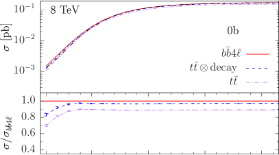
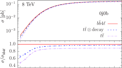
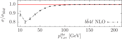
Figure 15: Integrated cross sections at 8 TeV in jet bins with zero $b$-jets as a function of the jet-$p_{\rm T}$ threshold. The left plot is inclusive with respect to extra jet radiation ($n_{j}{}\geq n_{b}{}=0$), while the right plot is exclusive  ($n_{j}=n_{b}=0$). Absolute predictions and ratios as in Fig. 14.

Jet-binning and jet-veto effects are studied in Figures 15–16. For this analysis we apply again the lepton selection cuts of Eq. (20) and, at variance with the $b$-jet definition in Section 6, we identify as $b$-jets those jets containing at least a $b$- or $\bar{b}$-flavoured hadron, irrespectively of its hardness. Events are categorised according to the number of (light or heavy-flavour) jets, $n_{j}$, and to the number of $b$-jets, $n_{b}$, in the rapidity range $|\eta|<2.5$, while we vary the jet transverse-momentum threshold $p_{\rm\mathchoice{\displaystyle}{\scriptstyle}{\scriptscriptstyle}{\scriptscriptstyle}T,jet}^{\rm\mathchoice{\displaystyle}{\scriptstyle}{\scriptscriptstyle}{\scriptscriptstyle}thr}$ that defines jets.

In Fig. 15, to investigate the effect of a $b$-jet veto, the integrated cross sections is plotted versus the jet-veto threshold, $p_{\rm\mathchoice{\displaystyle}{\scriptstyle}{\scriptscriptstyle}{\scriptscriptstyle}T,jet}^{\rm\mathchoice{\displaystyle}{\scriptstyle}{\scriptscriptstyle}{\scriptscriptstyle}thr}$. In the left plot the veto acts only on $b$-jets ($n_{j}{}\geq n_{b}{}=0$), while in the right plot a veto against light and $b$-jets is applied ($n_{j}{}=n_{b}{}=0$). For $p_{\rm\mathchoice{\displaystyle}{\scriptstyle}{\scriptscriptstyle}{\scriptscriptstyle}T,jet}^{\rm\mathchoice{\displaystyle}{\scriptstyle}{\scriptscriptstyle}{\scriptscriptstyle}thr}{}\gtrsim 80$ GeV the vetoed cross section is dominated by $t\bar{t}$ production and quickly converges towards the inclusive result. In this region we observe few-percent level agreement between the $t\bar{t}\,\otimes\,$decay and $b\bar{b}4\ell$ predictions, while the on-shell $t\bar{t}$ prediction features a 10% deficit due to the missing single-top topologies. Reducing the jet-veto scale increases this deficit up to $-30\%$ in the case of the inclusive $n_{b}{}=0$ cross section. This finding is well consistent with the size of finite-width effects reported in Ref. Cascioli:2013wga . In the case of the exclusive zero-jet cross section ($n_{j}{}=n_{b}{}=0$, shown on the right) the deficit of the $t\bar{t}$ prediction is even more pronounced and reaches up to $-50\%$ at $p_{\rm\mathchoice{\displaystyle}{\scriptstyle}{\scriptscriptstyle}{\scriptscriptstyle}T,jet}^{\rm\mathchoice{\displaystyle}{\scriptstyle}{\scriptscriptstyle}{\scriptscriptstyle}thr}{}=10$ GeV. Also the $t\bar{t}\,\otimes\,$decay results feature a similar, although less pronounced, deficit as the $t\bar{t}$ ones in the soft region. This can be attributed to the fact that initial-state radiation in both, the hvq and ttb_NLO_dec, generators is computed with on-shell tops, and thus overestimates the radiation produced near the single-top kinematic region.

Matching and pure shower effects are illustrated in the lower frames of Fig. 15. Both in the inclusive ($n_{j}{}>n_{b}{}=0$) and exclusive ($n_{j}{}=n_{b}{}=0$) case we observe that, down to 20 GeV, NLO+PS predictions feature an increasingly strong enhancement with respect to fixed-order ones. This can be attributed to shower-induced losses of $b$-jet transverse momentum. In the exclusive case ($n_{j}{}=n_{b}{}=0$) this enhancement is somewhat milder, which we tentatively attribute to the interplay of parton shower radiation with the additional light-jet veto.

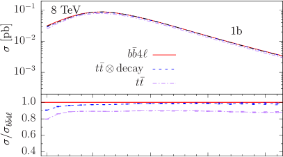
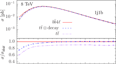
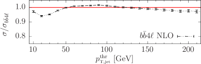
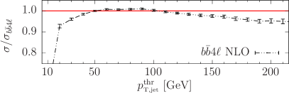
Figure 16: Integrated cross sections at 8 TeV in jet bins with one $b$-jet as a function of the jet-$p_{\rm T}$ threshold. The left plot is inclusive with respect to extra jet radiation ($n_{j}{}\geq n_{b}{}=1$), while the right plot is exclusive ($n_{j}=n_{b}=1$). Absolute predictions and ratios as in Fig. 14.

In Fig. 16 we plot the cross section with exactly one $b$-jet above the threshold $p_{\rm\mathchoice{\displaystyle}{\scriptstyle}{\scriptscriptstyle}{\scriptscriptstyle}T,jet}^{\rm\mathchoice{\displaystyle}{\scriptstyle}{\scriptscriptstyle}{\scriptscriptstyle}thr}$, i.e. we veto additional $b$-jets above this threshold. Again, inclusive results ($n_{j}{}\geq n_{b}{}=1$, shown on the left) are compared with exclusive ones ($n_{j}{}=n_{b}{}=1$, shown on the right). The one-$b$-jet bin is typically used in $Wt$ single-top analyses. Similarly as for the zero-$b$-jet case, the difference between the $b\bar{b}4\ell$ and $t\bar{t}$ results points to an increasingly important single-top contribution at small $p_{\rm\mathchoice{\displaystyle}{\scriptstyle}{\scriptscriptstyle}{\scriptscriptstyle}T,jet}^{\rm\mathchoice{\displaystyle}{\scriptstyle}{\scriptscriptstyle}{\scriptscriptstyle}thr}{}$. Its quantitative impact is consistent with the fixed-order results of Ref. Cascioli:2013wga , and at $p_{\rm\mathchoice{\displaystyle}{\scriptstyle}{\scriptscriptstyle}{\scriptscriptstyle}T,jet}^{\rm\mathchoice{\displaystyle}{\scriptstyle}{\scriptscriptstyle}{\scriptscriptstyle}thr}{}=30$ GeV it amounts to about 10% and $20\%$, respectively, in the inclusive and exclusive cases. Similarly as for the zero-$b$-jet case, $t\bar{t}\,\otimes\,$decay predictions feature a qualitatively similar but quantitatively less pronounced deficit with respect to the $b\bar{b}4\ell$ predictions. Matching and shower effects turn out to be rather mild in the inclusive case, probably due to the fact that the absolute distribution is not particularly steep in the limit of small transverse momentum. In contrast, the exclusive one-jet cross section ($n_{j}{}=n_{b}{}=1$) is much more sensitive to the jet-veto scale, which leads to sizable matching and shower effects at small $p_{\rm\mathchoice{\displaystyle}{\scriptstyle}{\scriptscriptstyle}{\scriptscriptstyle}T,jet}^{\rm\mathchoice{\displaystyle}{\scriptstyle}{\scriptscriptstyle}{\scriptscriptstyle}thr}$.

In summary, jet-vetoed cross sections can involve enhanced single-top contributions that are completely missing in the $t\bar{t}$ predictions obtained with the hvq generator while they are significantly underestimated in the $t\bar{t}\,\otimes\,$decay predictions of the ttb_NLO_dec generator, where single-top contributions are implemented via LO reweighting Campbell:2014kua . In practice such a reweighting approach ceases to work in phase-space regions far away from the double-resonant region.

8 Conclusions

In this paper we have presented the first Monte Carlo generator that provides a fully consistent NLO+PS simulation of $t\bar{t}$ production and decay in the different-flavour dilepton channel, including all finite-width and interference effects. This new generator, dubbed ${\tt bb4l}$, is based on the full NLO matrix elements for the process $pp\to\ell^{+}\nu_{\mathchoice{\displaystyle}{\scriptstyle}{\scriptscriptstyle}{\scriptscriptstyle}\ell}\,l^{-}\bar{\nu}_{\mathchoice{\displaystyle}{\scriptstyle}{\scriptscriptstyle}{\scriptscriptstyle}l}\,b\,\bar{b}$. This guarantees NLO accuracy in $t\bar{t}$ production and decay, as well as the exact treatment of spin correlations and off-shell effects in top decay. Top resonances are dressed with quantum corrections, and also non-factorisable corrections associated with the interference of radiation in production and decays are taken into account. Bottom-quark masses are consistently included, which is quite important for the accurate modelling of $b$-quark fragmentation. Moreover, finite $b$-quark masses permit to avoid collinear singularities from initial- or final-state $g\to b\,\bar{b}$ splittings. This allows for $W^{+}W^{-}b\bar{b}$ simulations in the full phase space, including regions with unresolved $b$ quarks, which are indispensable for the simulation of top backgrounds in the presence of jet vetoes. It moreover provides a unified NLO description of $t\bar{t}$ and single-top $Wt$ production, including their quantum interference.

The technical problems that arise from infrared subtractions and NLO+PS matching in the presence of top-quark resonances are addressed by means of the fully general resonance-aware matching method that was proposed in Ref. Jezo:2015aia and implemented in the POWHEG-BOX-RES framework. This framework, besides allowing for a consistent matching to shower Monte Carlo generators, also ameliorates the efficiency of infrared subtraction and phase-space integration in a drastic way, and allows for a factorised treatment of NLO radiation in off-shell top production and decays. This represents a significant improvement (especially for what concerns top decays) with respect to the case where NLO+PS matching is applied to a single QCD emission.

Technically, the ${\tt bb4l}$ generator was realised by implementing OpenLoops matrix elements in the POWHEG-BOX framework. To this end we have developed a new and fully flexible interface, which allows one to set up POWHEG-BOX+OpenLoops NLO+PS generators for any desired process in a rather straightforward way.

We have carried out a thorough study of the impact of the resonance-aware method. To this end, we have compared our results with those obtained after disabling the resonance-aware formalism in such a way that the bb4l generator becomes fully equivalent to a traditional POWHEG-BOX-V2 implementation. On the one hand we observed that ignoring resonance structures can deteriorate the performance of the generator up to the point of rendering it unusable. On the other hand, we observed considerable distortions in the reconstructed mass of the top resonances with respect to the full resonance-aware result. In essence, the mass distribution becomes wider around the peak and slightly shifted. We were able to track the origin of these effects to two competing causes: the generation of radiation performed by POWHEG, that is considerably modified in the resonance-aware method, and the generation of radiation in the shower stage, where the shower Monte Carlo, being unaware of which groups of particles arise from the same resonance, tends to widen the resonance peaks. We have also shown that it does not seem to be possible to remedy this last problem by reconstructing the resonance structure on the basis of simple kinematic guesses.

Much attention was dedicated to the comparison of the new ${\tt bb4l}$ generator and the ttb_NLO_dec generator of Ref. Campbell:2014kua . Both are capable of handling NLO spin correlations and radiation in top decays. However, off-shell effects are only computed at LO in ttb_NLO_dec by reweighting the NLO cross section using the ratio of the full off-shell Born cross section divided by its zero-width approximation. These two generators are expected to provide similar results in the vicinity of top resonances. In fact, in this region, we find only modest differences between the two. In particular, the top virtuality distribution and distributions involving $b$ jets are in reasonably good agreement. Slightly larger differences are found in distributions involving $B$ hadrons, like for example, the $B$ fragmentation function, in the top-decay frame.

A section of this work was dedicated to a comparison against the hvq generator, which has been heavily used by the LHC experimental collaborations for the generation of $t\bar{t}$ samples in both Run I and Run II. Close to the mass peak, bb4l and hvq predictions are fairly consistent, but the agreement is quickly spoiled as one moves towards off-shell regions. Furthermore, the ratio of the hvq to the bb4l results exhibits a negative slope across the resonance peak, and we found that the average virtuality of the top resonance in a window of $\pm 30$ GeV around the peak differs by about 0.5 GeV for the two generators. This calls for dedicated studies of the implications of resonance-aware matching in the context of precision $m_{t}$-measurements. More sizable differences have been observed in the structure of the associated $b$-jets, the bb4l generator leading consistently to narrower jets and a harder fragmentation function for the associated $B$ hadron. The above findings should be interpreted by keeping in mind that within the hvq generator radiation in top decays is solely handled by Pythia8, with matrix-element corrections turned on by default. These matrix-element corrections should improve the overall agreement between hvq and bb4l, and we have verified that disabling them leads to much more pronounced differences between the two generators.

We have included in this work an indicative comparative study of jet-veto effects when using the bb4l, ttb_NLO_dec and hvq generators. In the presence of jet vetoes, the hvq generator alone is clearly not adequate, since it misses the essential component of associated $Wt$ production. Perhaps surprisingly, it turns out that also the ttb_NLO_dec generator does not perform sufficiently well. Since $Wt$ production effects are included in this generator only at the level of a leading-order reweighting, we are led to conclude that the lack of NLO accuracy in the simulation of $Wt$ contributions limits the usability of the ttb_NLO_dec generator in single-top enriched regions. We stress however that the issue of jet-veto effects is complex, and deserves a dedicated future study.

The theoretical improvements implemented in the ${\tt bb4l}$ generator are relevant for phenomenological studies and experimental analysis that depends on the kinematic details of top-decay products. In particular, this new generator is ideally suited for precision determinations of the top-quark mass, for measurements of $Wt$ production, and for analyses where $t\bar{t}$ and $Wt$ production are subject to jet vetoes. The exact treatment of off-shell and non-resonant effects is also important for top backgrounds in Higgs and BSM studies based on kinematic selections with high missing energy or boosted $b\bar{b}$ pairs.

Appendix A Technical details

In this appendix we detail the technical improvements to the POWHEG-BOX-RES framework that have been implemented in order to allow for the implementation of $pp\,\to\,\ell^{+}\nu_{\mathchoice{\displaystyle}{\scriptstyle}{\scriptscriptstyle}{\scriptscriptstyle}\ell}\,l^{-}\bar{\nu}_{\mathchoice{\displaystyle}{\scriptstyle}{\scriptscriptstyle}{\scriptscriptstyle}l}\,b\,\bar{b}$.

A.1 Automatic generation of resonance histories

The algorithm for finding the resonance histories is at present at an experimental level. It has been kept as simple and straightforward as possible in order to allow for future improvements and modifications.

The algorithm begins with the lists of particle flavours specified in the user process routine init_processes, where the arrays flst_born and flst_real are filled. At variance with the POWHEG-BOX-V2 version, one also has to specify the length of each flavour list in the arrays. The lengths are stored in the arrays flst_bornlength and flst_reallength. For the process we are considering here (and in most cases) the lengths have all the same values (8 for the Born process and 9 for the real). At this stage, no resonance information is provided for the flavour lists, so the lists of resonance pointers (flst_bornres and flst_realres) remain initialized to zero, and the user does not need to modify them. The powers of the strong and weak coupling constants in the Born amplitudes (res_powst and res_powew) must instead be initialized by the user-process routines. At the moment we do not consider the possibility of having multiple Born-level processes with different orders of the strong and weak coupling constants. This may be required when considering mixed strong and electromagnetic radiation being generated with the POWHEG method, and will require minor modification of the code.

The algorithm proceeds recursively: intermediate particles are added at the end of the flavour list, and the pointers associated with the particles that arise from their splitting are appropriately set.

As an example, we consider the production of a $W$ in association with a quark antiquark pair $d\bar{u}\to e^{-}{\bar{\nu}_{e}}u\bar{u}$, with two powers of the strong coupling constant and two powers of the weak one. The input consists of the following arguments

  flav    = [1, -2, 11, -12,  2, -2],
  flavres = [0,  0,  0,   0,  0,  0],
  powst   = 2,
  powew   = 2.

The algorithm proceeds as follows:

• The first particle is kept fixed. The second particle is charge reversed, so that the process looks like the decay of the first particle into the remaining ones. At this stage we then have

    flav    = [1, 2, 11, -12,  2, -2],
    flavres = [0, 0,  0,   0,  0,  0],
    powst   = 2,
    powew   = 2.
  

• We look through all (ordered) pairs of particles, excluding the first one, that have flavres equal to zero, and that can be merged into a single particle via a strong or weak interaction vertex. In the example at hand, we would find several cases: the second and last entry (a $u$ and a $\bar{u}$) merged into a gluon, a photon or a $Z$; for the third and fourth entry (an electron and its anti-neutrino) merged into a $W^{-}$; the last two entries (a $u$ and $\bar{u}$) merged into a gluon, a photon or a $Z$.

• For each found possible merging, we prepare a new input for the recursive procedure, with a new flavour list including the merged particle and updated values of the resonance pointers and of the power of the couplings. In our example, after the $e^{-}{\bar{\nu}}$ pair is merged into a $W^{-}$, the new input for the recursive procedure looks like this

    flav    = [1, 2, 11, -12,  2, -2, -24],
    flavres = [0, 0,  7,   7,  0,  0,   0],
    powst   = 2,
    powew   = 1.
  

  Notice that now the flavres third and fourth entries (the $e^{-}$ and ${\bar{\nu}}$) contain pointers to their mother resonance (the $W^{-}$), added in the seventh position. The value of powew has been updated, since one electroweak coupling was used for the $W^{-}$ splitting, and only one is left. Notice also that there are cases where the same particles can merge into a different one, as for the $u$ and $\bar{u}$ merging case, and all these new inputs are passed to the recursive resonance-searching algorithm.

• By proceeding with the recursion, we will reach a point when no further merging is possible. Following the example at hand, we may find that the $u{\bar{u}}$ pair is merged into a gluon

    flav    = [1, 2, 11, -12,  2, -2, -24,  0],
    flavres = [0, 0,  7,   7,  8,  8,   0,  0],
    powst   = 1,
    powew   = 1,
  

  followed by a $gu$ merging into a $u$

    flav    = [1, 2, 11, -12,  2, -2, -24,  0, 2],
    flavres = [0, 9,  7,   7,  8,  8,   0,  9, 0],
    powst   = 0,
    powew   = 1,
  

  finally followed by a $uW^{-}$ merging into a $d$

    flav    = [1, 2, 11, -12,  2, -2, -24, 21,  2, 1],
    flavres = [0, 9,  7,   7,  8,  8,  10,  9, 10, 0],
    powst   = 0,
    powew   = 0.
  

  At this point three conditions are checked: whether no pairs can be further merged, whether no more powers of the coupling constants are available, and whether the last added particle coincides with the first one, meaning that all outgoing particles have been merged into the incoming one. If any of these conditions are not met, the configuration is abandoned.

The list just found represents a tree diagram for the process at hand. As such, there is always a unique path in the tree that joins any two external particles. The path joining the two incoming particle is the $t$-channel one. It can be found starting from particle 2 and going recursively through its ancestors, until particle 1 is reached.

The list is processed further, by the subroutine clean_resonance_structure, that performs the following operations. It first examines the $t$-channel structure of the flavour list. If it finds a $t$-channel fermion line that emits two electroweak bosons ($W$, $Z$ or $H$) that can directly couple to each other trough a triple-boson vertex, with any intermediate emission of photons or gluons, it abandons the configuration. This is because another configuration with a richer resonance structure must exist, i.e. the structure where the two electroweak bosons arise from the decay of a single electroweak boson, with splittings involving the trilinear vector coupling, or the Higgs coupling to a vector boson. This richer configuration is well-suited to represent the one where the two electroweak bosons do not originate from another electroweak boson, and thus the latter configurations need not be considered. It then carries out a similar operation on $s$-channel lines. If we find a fermion line that emits two electroweak bosons, there must be a richer configuration where the two bosons originate from a single electroweak boson, and we thus abandon this configuration. Care is taken to handle the special case when the fermion line becomes a top quark, since the top is treated as a resonance, and the emission of a Higgs from the fermion line, since it must come from a top, in this case.

After the elimination procedure is carried out, all $t$-channel resonance entries, and all $s$-channel resonance entries corresponding to a massless particle are deleted from the list. The list is then put in a standard form: the resonances are moved just after the two incoming particles, and the final-state particles follow. The clean_resonance_structure exits. If the examined flavour structure is to be kept, the program calls a subroutine that stores it in a temporary array structure, provided there are no other equivalent configurations already stored. Once all configurations are found and stored, the subroutine pwhg_res_histos_born or pwhg_res_histos_real is called, and the configurations are transferred from the temporary storage to the global arrays flst_born* or flst_real*, that are overwritten with the Born and real flavour structure including resonance-history information.

The procedure that we have illustrated so far should be appropriate for most Standard Model processes. We checked that it works also in the case of single-top production studied in Ref. Jezo:2015aia , by replacing the hand-written resonance histories that we used there with those automatically generated with the procedure presented here.

A.2 Colour assignment

In the POWHEG-BOX, colour assignment is mainly performed at the level of the underlying Born process. Given a Born flavour configuration and kinematics, one considers the colour subamplitudes that contribute to the squared Born amplitude, computed in the large colour limit. A color flow is then chosen with a probability proportional to the values of the subamplitudes, for that particular phase-space point. The POWHEG-BOX then generates the QCD radiation for a particular collinear region, through the splitting process. The colour configuration for the generated real-emission amplitude is obtained from the one of the underlying Born by attaching the colour flow that corresponds to that splitting.

Contributions that do not have singular regions (i.e. regular contributions) are instead treated as the Born term itself. In Ref. Campbell:2012am a corresponding interface was developed such that this colour information could be extracted from MadGraph4. In Section A.3, we describe an analogous implementation in OpenLoops.

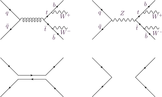
Figure 17: Different resonance histories (top) for identical processes, and associated colour flows (bottom).

When resonance histories are being considered, a modification of this scheme becomes necessary. In fact, the randomly generated colour assignment may not be compatible with the resonant structure being considered. Consider for example the process $q\bar{q}\to q\bar{q}VV$, where $V$ is a vector boson, illustrated in Fig. 17. If the process proceeds via the exchange of a gluon in the $s$-channel, then the corresponding colour flow is illustrated in the bottom-left diagram in the figure, and initial- and final-state quarks are colour connected. Whereas if the exchanged particle in the $s$-channel is a colourless vector boson, then the color flow is depicted in the bottom-right diagram, where it is evident that initial- and final-state quarks are not colour connected, but there is a colour connection between the quarks in the initial state, and another colour connection between the quarks in the final state.

In the POWHEG-BOX framework, colour assignment is independent of the resonance structure, and thus one may end up assigning the colour flow in the left of the figure to the resonance history on the right, or vice-versa. In order to remedy to this, we keep generating random colour configurations, and accept the first one that is compatible with the resonance history.

A.3 OpenLoops interface and settings

The OpenLoops program is based on a fast numerical recursion for the generation of tree and one-loop scattering amplitudes Cascioli:2011va . Combined with the OPP reduction method Ossola:2006us implemented in CutTools Ossola:2007ax and the scalar one-loop library OneLOop vanHameren:2010cp , or with the tensor integral reduction methods Denner:2002ii ; Denner:2005nn ; Denner:2010tr implemented in COLLIER Denner:2016kdg , the employed recursion permits to achieve very high CPU performance and a high degree of numerical stability. The small fraction of numerically unstable one-loop matrix elements is automatically detected and rescued through re-evaluation with CutTools in quadruple precision.

The new POWHEG-BOX+OpenLoops interface is implemented via a Fortran90 module called openloops_powheg, which is included in the POWHEG-BOX-RES framework. Internally the POWHEG-BOX+OpenLoops framework automatically compiles, loads and manages all required OpenLoops amplitude libraries. The new interface provides the subroutines openloops_born, openloops_real, and openloops_virtual with interfaces identical to the corresponding POWHEG-BOX routines setborn, setreal, and setvirtual. In particular the openloops_born routine returns, besides the squared tree-level amplitude $\mathcal{B}$, the corresponding colour- and spin-correlated tree-level amplitudes $\mathcal{B}_{ij}$ and $\mathcal{B}_{\mu\nu}$ in the format required by the POWHEG-BOX Alioli:2010xd . Additionally, the interface provides the routines openloops_init, openloops_borncolour and openloops_realcolour. The former synchronizes all parameters between OpenLoops and the POWHEG-BOX and should be called at the end of the init_processes subroutine of the POWHEG-BOX. The latter two provide the required colour information as outlined in Section A.2, i.e. they return a colour-flow of the squared Born and real matrix elements in the large colour limit, on a probabilistic basis. Since the probability priors are determined from the colour-flow decomposition of the corresponding matrix elements at a given phase-space point, the colour-trace basis employed internally in OpenLoops is converted into a color-flow basis.

Several OpenLoops internal options and switches can be passed directly from the powheg.input file to the code. In particular, OpenLoops offers the possibility to switch between the tensor-integral reduction methods implemented in COLLIER and OPP reduction methods implemented in CutTools. By default COLLIER is used, while inserting the line

olpreset 1

in the powheg.input file, reduction via CutTools can be selected. In a similar way, inserting the line

olverbose <OpenLoops verbosity level>

allows to select the verbosity level of OpenLoops.

While all relevant input parameters are automatically passed by POWHEG-BOX to OpenLoops, further internal OpenLoops parameters can be set directly via the routine (member of the Fortran90 module openloops)

set_parameter(parameter, value)
  character(*), intent(in) :: parameter
  TYPE, intent(in) :: value

Here, TYPE can either be integer, double or character(*) according to the parameter to be set, as detailed on http://openloops.hepforge.org/parameters.html.

Implementation of new processes

In order to set up a new processes within the POWHEG-BOX+OpenLoops framework, one should run the script <POWHEG-BOX-RES>/COMMON/OpenLoopsStuff/generate_process.py with the following arguments

./generate_process.py <library name> -order_ew=<m> -order_qcd=<n> -name=<..>

Here, <library name> corresponds to the OpenLoops amplitude library of the desired process and <m> and <n> denote the order of the Born cross section, $\mathcal{O}(\alpha_{\mathchoice{\displaystyle}{\scriptstyle}{\scriptscriptstyle}{\scriptscriptstyle}\rm S}^{n}\alpha_{\mathchoice{\displaystyle}{\scriptstyle}{\scriptscriptstyle}{\scriptscriptstyle}\rm EM}^{m})$, in terms of powers of the strong and weak couplings. This will setup a rudimentary POWHEG-BOX process structure within the directory <POWHEG-BOX-RES>/COMMON/<name>. For example the call

./generate_process.py pplnjjj -order_ew=2 -order_qcd=3 -name=Wjjj

will yield the structure for an NLO+PS generator including all required tree and one-loop amplitudes for $pp\to W(\to\ell\nu)+3\leavevmode\nobreak\ {\rm jet}$ production.

A user has only to provide the list of contributing flavour structures of the Born and real subprocesses in the init_processes.f file and the number of intermediate resonances in the nlegborn.h file. An automatic generation of these structures is currently being validated and will soon be included. Currently NLO QCD corrections to any SM process are supported by this interface, while NLO electroweak corrections will follow in the future.

A.4 Optimising the virtual corrections

Fixed-order NLO calculations

If one is interested in fixed-order NLO results, the most CPU-demanding contributions come from the computation of the real graphs, that also implement the cancellation of the collinear and soft singularities. In the POWHEG-BOX-RES code there are options to separate the virtual contribution from the rest, in such a way that it can be computed with an accuracy that matches the one of the real contribution, thus saving computer time. More specifically, the code can be run twice: in the first run, the user can set the flag novirtual to 1 in the powheg.input file. In this way, no call to the calculation of the virtual corrections is done, and the corresponding distributions do not contain the virtual corrections (plus other soft contributions). The code is then rerun by using the same importance sampling grids used in the first run, with the flag virtonly set to 1 and with lower statistics with respect to the previous run. In this way, the virtual contributions are called fewer times with respect to the Born and real contributions of the first run. Finally, the kinematic distributions obtained in the two steps can then be combined. Details and examples for this procedure are included in the release of the code.

Generation of Monte Carlo events

If one is interested in generating Monte Carlo events, it is more convenient to avoid the computation of the virtual corrections for the large number of events that are vetoed during the generation. This can be done, provided one renounces to generating events with constant weight. In essence, we generate events with settings such that the virtual contribution is not computed, but the cross section and the distributions are sufficiently similar to the exact result. The events are then reweighted with the full cross section including the virtual contribution. With this procedure, the virtual contribution is computed only once for each generated event, instead of the several tens of event that are computed and then vetoed in a standard run. In order to do so, one inserts in the powheg.input file the lines

for_reweighting 1
rwl_file ’-’
<initrwgt>
<weight id=’xx’>  some reweight info </weight>
...
</initrwgt>

and the program generates events with uniform weight with no virtual corrections. For each <weight line, a new weight is generated and added to the event. These weights are all computed with the inclusion of the virtual corrections.

We would like to remark an additional technical issue: the subtraction term in case of a massive fermion emitter (i.e. the subtraction term corresponding to the soft singularity in the $b\to bg$ splitting) is modified in such a way that it becomes closer to the $P_{qg}(z)$ Altarelli-Parisi splitting function (that is to say, we give it a weight $(1+z^{2})/(1-z)$ rather than the original weight $2/(1-z)$). In fact, we found that if we do not include this modification, the kinematic distributions before reweighting (i.e. those with no soft-virtual contributions) can develop relatively large, negative values near the top-mass peak. After reweighting we do get back the correct results. However, reweighting coefficients can be very large or negative with the original subtraction term, while, with the modified one, we get sensible distributions even before reweighting, and no large reweighting factors.

Appendix B Phenomenological details

B.1 Kinematic guess of resonance structures

In this appendix we detail the kinematic procedure for the construction of resonance information from agnostic events, i.e. events where no resonance information is available.

We start at the Les Houches event level and modify each event as follows:

• The matching $l\nu$ pairs are assigned to the corresponding $W^{\pm}$ bosons, that are added to the event record, with the corresponding kinematics: $p_{\mathchoice{\displaystyle}{\scriptstyle}{\scriptscriptstyle}{\scriptscriptstyle}W^{+}}=(p_{\mathchoice{\displaystyle}{\scriptstyle}{\scriptscriptstyle}{\scriptscriptstyle}\ell^{+}}+p_{\mathchoice{\displaystyle}{\scriptstyle}{\scriptscriptstyle}{\scriptscriptstyle}\nu})$ and $p_{\mathchoice{\displaystyle}{\scriptstyle}{\scriptscriptstyle}{\scriptscriptstyle}W^{-}}=(p_{\mathchoice{\displaystyle}{\scriptstyle}{\scriptscriptstyle}{\scriptscriptstyle}l^{-}}+p_{\mathchoice{\displaystyle}{\scriptstyle}{\scriptscriptstyle}{\scriptscriptstyle}\bar{\nu}})$

• If no parton is radiated, or if the radiated parton is not a gluon, then the top resonances can only be formed by pairing a $W$ and the corresponding $b$ (i.e. no radiation from top quarks is present). In this case we compute the resonance enhancement factors

  $$f_{t} = \frac{m_{t}^{4}}{\left[(p_{\mathchoice{\displaystyle}{\scriptstyle}{\scriptscriptstyle}{\scriptscriptstyle}b}+p_{\mathchoice{\displaystyle}{\scriptstyle}{\scriptscriptstyle}{\scriptscriptstyle}W^{+}})^{2}-m_{t}^{2}\right]^{2}+(\Gamma_{t}m_{t})^{2}}\,,$$ (22)

  $$f_{\bar{t}} = \frac{m_{t}^{4}}{\left[(p_{\mathchoice{\displaystyle}{\scriptstyle}{\scriptscriptstyle}{\scriptscriptstyle}\bar{b}}+p_{\mathchoice{\displaystyle}{\scriptstyle}{\scriptscriptstyle}{\scriptscriptstyle}W^{-}})^{2}-m_{t}^{2}\right]^{2}+(\Gamma_{t}m_{t})^{2}}\,,$$ (23)

  $$f_{\mathchoice{\displaystyle}{\scriptstyle}{\scriptscriptstyle}{\scriptscriptstyle}Z} = \frac{m_{\mathchoice{\displaystyle}{\scriptstyle}{\scriptscriptstyle}{\scriptscriptstyle}z}^{4}}{\left[(p_{\mathchoice{\displaystyle}{\scriptstyle}{\scriptscriptstyle}{\scriptscriptstyle}W^{+}}+p_{\mathchoice{\displaystyle}{\scriptstyle}{\scriptscriptstyle}{\scriptscriptstyle}W^{-}})^{2}-m_{\mathchoice{\displaystyle}{\scriptstyle}{\scriptscriptstyle}{\scriptscriptstyle}Z}^{2}\right]^{2}+(\Gamma_{\mathchoice{\displaystyle}{\scriptstyle}{\scriptscriptstyle}{\scriptscriptstyle}Z}m_{\mathchoice{\displaystyle}{\scriptstyle}{\scriptscriptstyle}{\scriptscriptstyle}Z})^{2}}\,.$$ (24)

  We then generate a random number $r$: if $r<f_{\mathchoice{\displaystyle}{\scriptstyle}{\scriptscriptstyle}{\scriptscriptstyle}Z}/(f_{t}\,f_{\bar{t}}\,+f_{\mathchoice{\displaystyle}{\scriptstyle}{\scriptscriptstyle}{\scriptscriptstyle}Z})$ we assume that the event has a resonance history with the $W$ pair arising from an intermediate $s$-channel $Z$. If not, the $W$’s are paired with the corresponding $b$ and assigned to a top and an anti-top. In both cases, the Les Houches event record is adjusted accordingly.

• If the radiated parton is a gluon, besides the $f$ factors computed in the previous item, we compute

  $$f_{t}^{\mathchoice{\displaystyle}{\scriptstyle}{\scriptscriptstyle}{\scriptscriptstyle}(r)} = \frac{m_{t}^{4}}{\left[(p_{\mathchoice{\displaystyle}{\scriptstyle}{\scriptscriptstyle}{\scriptscriptstyle}b}+p_{\mathchoice{\displaystyle}{\scriptstyle}{\scriptscriptstyle}{\scriptscriptstyle}W^{+}}+p_{\mathchoice{\displaystyle}{\scriptstyle}{\scriptscriptstyle}{\scriptscriptstyle}g})^{2}-m_{t}^{2}\right]^{2}+(\Gamma_{t}m_{t})^{2}}\,,$$ (25)

  $$f_{{\bar{t}}}^{\mathchoice{\displaystyle}{\scriptstyle}{\scriptscriptstyle}{\scriptscriptstyle}(r)} = \frac{m_{t}^{4}}{\left[(p_{\mathchoice{\displaystyle}{\scriptstyle}{\scriptscriptstyle}{\scriptscriptstyle}\bar{b}}+p_{\mathchoice{\displaystyle}{\scriptstyle}{\scriptscriptstyle}{\scriptscriptstyle}W^{-}}+p_{\mathchoice{\displaystyle}{\scriptstyle}{\scriptscriptstyle}{\scriptscriptstyle}g})^{2}-m_{t}^{2}\right]^{2}+(\Gamma_{t}m_{t})^{2}}\,.$$ (26)

  Furthermore, we also compute:

  • $p_{\mathchoice{\displaystyle}{\scriptstyle}{\scriptscriptstyle}{\scriptscriptstyle}T}^{\mathchoice{\displaystyle}{\scriptstyle}{\scriptscriptstyle}{\scriptscriptstyle}g}$: the gluon transverse-momentum relative to the beams;

  • $p_{\mathchoice{\displaystyle}{\scriptstyle}{\scriptscriptstyle}{\scriptscriptstyle}T,b/{\bar{b}}}^{\mathchoice{\displaystyle}{\scriptstyle}{\scriptscriptstyle}{\scriptscriptstyle}g}$: the gluon transverse-momentum relative to the outgoing $b$’s in the partonic CM system;

  • $p^{\mathchoice{\displaystyle}{\scriptstyle}{\scriptscriptstyle}{\scriptscriptstyle}g(r)}_{\mathchoice{\displaystyle}{\scriptstyle}{\scriptscriptstyle}{\scriptscriptstyle}T,b/{\bar{b}}}$: the gluon transverse-momentum relative to the outgoing $b$’s in the $t^{\mathchoice{\displaystyle}{\scriptstyle}{\scriptscriptstyle}{\scriptscriptstyle}(r)}/{\bar{t}}^{\mathchoice{\displaystyle}{\scriptstyle}{\scriptscriptstyle}{\scriptscriptstyle}(r)}$ frame built under the assumption that radiation arises from top/anti-top decay.

• We compute the following weights

  $$w_{\mathchoice{\displaystyle}{\scriptstyle}{\scriptscriptstyle}{\scriptscriptstyle}Z}=\frac{f_{\mathchoice{\displaystyle}{\scriptstyle}{\scriptscriptstyle}{\scriptscriptstyle}Z}}{\left(p_{\mathchoice{\displaystyle}{\scriptstyle}{\scriptscriptstyle}{\scriptscriptstyle}T}^{\mathchoice{\displaystyle}{\scriptstyle}{\scriptscriptstyle}{\scriptscriptstyle}g}\right)^{2}}+\frac{f_{\mathchoice{\displaystyle}{\scriptstyle}{\scriptscriptstyle}{\scriptscriptstyle}Z}}{\left(p_{\mathchoice{\displaystyle}{\scriptstyle}{\scriptscriptstyle}{\scriptscriptstyle}T,b}^{\mathchoice{\displaystyle}{\scriptstyle}{\scriptscriptstyle}{\scriptscriptstyle}g}\right)^{2}}+\frac{f_{\mathchoice{\displaystyle}{\scriptstyle}{\scriptscriptstyle}{\scriptscriptstyle}Z}}{\left(p_{\mathchoice{\displaystyle}{\scriptstyle}{\scriptscriptstyle}{\scriptscriptstyle}T,\bar{b}}^{\mathchoice{\displaystyle}{\scriptstyle}{\scriptscriptstyle}{\scriptscriptstyle}g}\right)^{2}}\,,$$ (27)

  $$w_{\mathchoice{\displaystyle}{\scriptstyle}{\scriptscriptstyle}{\scriptscriptstyle}t{\bar{t}}}=\frac{f_{\mathchoice{\displaystyle}{\scriptstyle}{\scriptscriptstyle}{\scriptscriptstyle}t}\,f_{\mathchoice{\displaystyle}{\scriptstyle}{\scriptscriptstyle}{\scriptscriptstyle}\bar{t}}}{\left(p_{\mathchoice{\displaystyle}{\scriptstyle}{\scriptscriptstyle}{\scriptscriptstyle}T}^{\mathchoice{\displaystyle}{\scriptstyle}{\scriptscriptstyle}{\scriptscriptstyle}g}\right)^{2}}\,,\qquad w_{\mathchoice{\displaystyle}{\scriptstyle}{\scriptscriptstyle}{\scriptscriptstyle}t}^{\mathchoice{\displaystyle}{\scriptstyle}{\scriptscriptstyle}{\scriptscriptstyle}(r)}=\frac{f_{\mathchoice{\displaystyle}{\scriptstyle}{\scriptscriptstyle}{\scriptscriptstyle}t}^{\mathchoice{\displaystyle}{\scriptstyle}{\scriptscriptstyle}{\scriptscriptstyle}(r)}}{\left(p^{\mathchoice{\displaystyle}{\scriptstyle}{\scriptscriptstyle}{\scriptscriptstyle}g(r)}_{\mathchoice{\displaystyle}{\scriptstyle}{\scriptscriptstyle}{\scriptscriptstyle}T,b}\right)^{2}}\,,\qquad w_{\mathchoice{\displaystyle}{\scriptstyle}{\scriptscriptstyle}{\scriptscriptstyle}\bar{t}}^{\mathchoice{\displaystyle}{\scriptstyle}{\scriptscriptstyle}{\scriptscriptstyle}(r)}=\frac{f_{\mathchoice{\displaystyle}{\scriptstyle}{\scriptscriptstyle}{\scriptscriptstyle}\bar{t}}^{\mathchoice{\displaystyle}{\scriptstyle}{\scriptscriptstyle}{\scriptscriptstyle}(r)}}{\left(p^{\mathchoice{\displaystyle}{\scriptstyle}{\scriptscriptstyle}{\scriptscriptstyle}g(r)}_{\mathchoice{\displaystyle}{\scriptstyle}{\scriptscriptstyle}{\scriptscriptstyle}T,\bar{b}}\right)^{2}}\,,$$ (28)

  corresponding to the following resonance histories:

  • the two $W$’s come from the intermediate $Z$ boson and the gluon is associated to initial- or final-state radiation (from the $b$’s);

  • the $W$’s and $b$’s come from a $t\bar{t}$ pair, and the gluon from initial-state radiation;

  • same as before but with the gluon from the top-resonance decay;

  • same as before but with the gluon from the antitop-resonance decay.

  If the colour of the $b$ is not consistent with the colour assigned to the gluon, the corresponding weight is set to zero. Then, a resonance history and gluon assignment are chosen among the four configurations considered here with probability proportional to the corresponding $w$ weight.

In order to validate this procedure, we stripped any resonance information from the Les Houches events of a resonance-aware res-singlerad sample, i.e. switching off the multiple-radiation scheme. We indicate the corresponding results with the label res-strip. Then, following the procedure outlined above, we added back guessed resonance information. The obtained result, labelled as res-strip-guess, is displayed in Fig. 18.

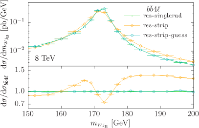
Figure 18: Comparison of the effect of removing resonance information and then adding it back according to a guess, based upon kinematics, in the invariant mass of the $W{j_{\rm\mathchoice{\displaystyle}{\scriptstyle}{\scriptscriptstyle}{\scriptscriptstyle}B}}$ system.

As we can see, the procedure for the kinematic construction of resonance information reproduces nicely the correct $W{j_{\rm\mathchoice{\displaystyle}{\scriptstyle}{\scriptscriptstyle}{\scriptscriptstyle}B}}$ peak.

B.2 Comparisons of shower veto schemes

When generating radiation from resonance decay, the traditional Les Houches generic-user process interface is no longer viable. In fact, the standard Boos:2001cv contemplates only a single scale (called scalup), and it requires that the shower does not generate any radiation harder than that scale at the production stage. Radiation in resonance decays remains, however, unrestricted, while our generator requires it to be vetoed either by the transverse momentum of the radiation generated by POWHEG in the decay process (allrad 1 case), or by the hardest radiation scale, irrespective of its origin (i.e. either from production or from resonance decay) in the allrad 0 case.

The default method for interfacing the bb4l generator to Pythia8 was taken from Ref. Campbell:2014kua , and it is described in appendix A of that paper. In essence, the procedure was to examine the showered event, compute the transverse momentum of Pythia8 radiation in top decays, and veto it if higher than the corresponding POWHEG one.

Pythia8 provides with its own mechanism for vetoing radiation from resonance decay. One should implement a virtual function canSetResonanceScale that returns a true value if Pythia8 is to use this mechanism. Furthermore, one should also implement a function scaleResonance that Pythia8 invokes in each event for each resonance, returning the scale for vetoing radiation in decay. We also implement this mechanism in our generator. It is activated by setting the flag pythiaveto 1 in the powheg.input file.

We show in Fig. 19

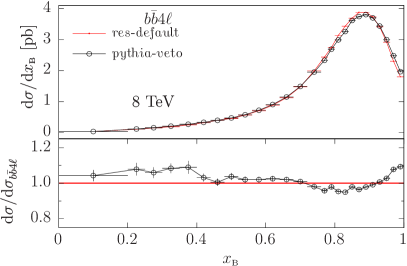
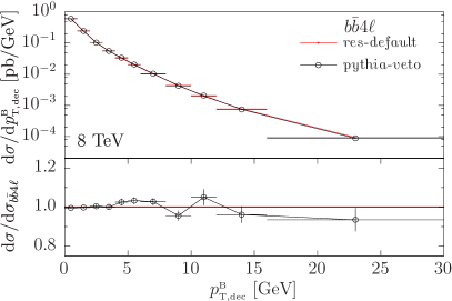
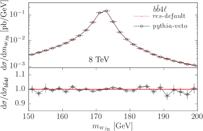
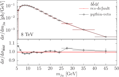
Figure 19: Comparison of two veto schemes on the $B$ fragmentation function, on $p^{\rm\mathchoice{\displaystyle}{\scriptstyle}{\scriptscriptstyle}{\scriptscriptstyle}B}_{\mathchoice{\displaystyle}{\scriptstyle}{\scriptscriptstyle}{\scriptscriptstyle}\rm T,dec}$, on the mass of the $W{j_{\rm\mathchoice{\displaystyle}{\scriptstyle}{\scriptscriptstyle}{\scriptscriptstyle}B}}$ system and on the mass of ${j_{\rm\mathchoice{\displaystyle}{\scriptstyle}{\scriptscriptstyle}{\scriptscriptstyle}B}}$ distributions.

the comparison of results obtained with the two veto mechanisms. In these plots, as well as in all the others that we have examined, we have found very good agreement between the two veto schemes. We notice that the difference in the ratio of the $m_{j_{\rm\mathchoice{\displaystyle}{\scriptstyle}{\scriptscriptstyle}{\scriptscriptstyle}B}}$ distribution at small masses (one of the few distributions where we found mild discrepancies) is taking place in a region where the cross section is getting small, and is thus of little relevance.

We conclude that the internal Pythia8 method for vetoing resonance radiation in decay is suitable for use with the bb4l generator, and we can thus recommend its use.

B.3 Impact of the multiple radiation scheme

Difference in $t\bar{t}$ observables induced by the multiple-radiation scheme of Eq. (6) were already discussed at length in Ref. Campbell:2014kua for the ttb_NLO_dec generator. It was found there that, by switching off the multiple-radiation scheme (allrad 0), radiation from top decays are mostly handled by the shower generator. In fact, the absolute hardest radiation is more often produced by the initial state, in part because of the larger colour charge, and in part due to the wider phase space available. Here we present some comparisons as a brief reminder of the relevant issues. In this section we apply our default cuts defined in Eqs. (19)–(20). We begin by showing in Fig. 20

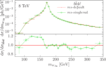
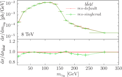
Figure 20: Invariant mass of the $W{j_{\rm\mathchoice{\displaystyle}{\scriptstyle}{\scriptscriptstyle}{\scriptscriptstyle}B}}$ (left) and of the $l{j_{\rm\mathchoice{\displaystyle}{\scriptstyle}{\scriptscriptstyle}{\scriptscriptstyle}B}}$ (right) systems. We compare NLO+PS resonance-aware predictions with (res-default) and without (res-singlerad) employing the multiple radiation scheme. In the ratio plot we illustrate relative deviations with respect to res-default.

the invariant mass distribution of the $W{j_{\rm\mathchoice{\displaystyle}{\scriptstyle}{\scriptscriptstyle}{\scriptscriptstyle}B}}$ and of the $l{j_{\rm\mathchoice{\displaystyle}{\scriptstyle}{\scriptscriptstyle}{\scriptscriptstyle}B}}$ systems. There is a good agreement between the two distributions, except for the region of low top virtuality in the left plot. On the other hand, observables that are sensitive to the $B$ and ${j_{\rm\mathchoice{\displaystyle}{\scriptstyle}{\scriptscriptstyle}{\scriptscriptstyle}B}}$ properties display larger differences, as can be seen in Fig. 21.

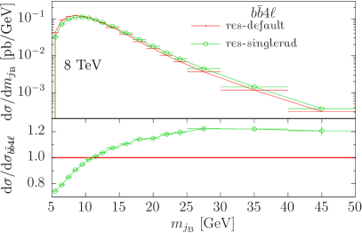
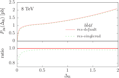
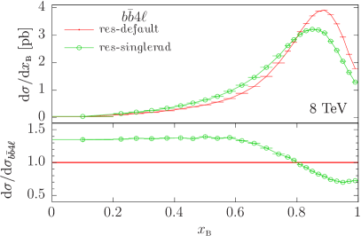
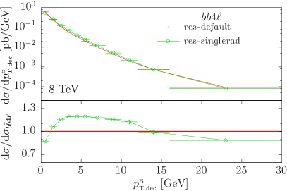
Figure 21: Mass (left top) and profile (right top) of the $b$-jet, ${j_{\rm\mathchoice{\displaystyle}{\scriptstyle}{\scriptscriptstyle}{\scriptscriptstyle}B}}$, and for the $B$ fragmentation function (left bottom) and transverse momentum distribution of the $B$ hadron in the top decay frame, $p^{\rm\mathchoice{\displaystyle}{\scriptstyle}{\scriptscriptstyle}{\scriptscriptstyle}B}_{\mathchoice{\displaystyle}{\scriptstyle}{\scriptscriptstyle}{\scriptscriptstyle}\rm T,dec}$ (right bottom). Absolute predictions and ratios as in Fig. 20.

In view of the large differences in the fragmentation function and $p^{\rm\mathchoice{\displaystyle}{\scriptstyle}{\scriptscriptstyle}{\scriptscriptstyle}B}_{\mathchoice{\displaystyle}{\scriptstyle}{\scriptscriptstyle}{\scriptscriptstyle}\rm T,dec}$ distribution, we compare in Fig. 22

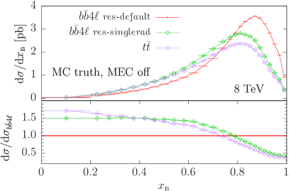
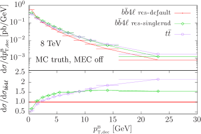
Figure 22: Predictions for the $B$ fragmentation function and transverse momentum distribution of the $B$ hadron in the top decay frame, $p^{\rm\mathchoice{\displaystyle}{\scriptstyle}{\scriptscriptstyle}{\scriptscriptstyle}B}_{\mathchoice{\displaystyle}{\scriptstyle}{\scriptscriptstyle}{\scriptscriptstyle}\rm T,dec}$ obtained with the bb4l generator in its default mode employing the multiple radiation scheme (res-default), without employing this scheme (res-singlerad) and corresponding predictions obtained with the hvq generator ($t\bar{t}$). In these predictions the top reference frame is determined according to the Monte Carlo truth (MC truth) and the $t\bar{t}$ predictions are obtained switching off matrix-elements corrections in Pythia8.

the same quantities computed using as reference frame the top quark at the level of Monte Carlo truth (“MC truth”, usually identified with the last top quark appearing in the shower output list) rather than the reconstructed top. We also add to this comparison the output of the hvq generator. In this last case, we switch off Pythia8 matrix element corrections (MEC), for the purpose of determining whether the use of our generator, even if the allrad feature is switched off, brings out some improvement with respect to a generic shower treatment of top decays. We see from the figures that by using the MC truth for the top reference frame brings the bb4l and res-singlerad results in better agreement, at least as far as the $p^{\rm\mathchoice{\displaystyle}{\scriptstyle}{\scriptscriptstyle}{\scriptscriptstyle}B}_{\mathchoice{\displaystyle}{\scriptstyle}{\scriptscriptstyle}{\scriptscriptstyle}\rm T,dec}$ distribution is concerned.

The comparison of the bb4l, res-singlerad and hvq results for the $p^{\rm\mathchoice{\displaystyle}{\scriptstyle}{\scriptscriptstyle}{\scriptscriptstyle}B}_{\mathchoice{\displaystyle}{\scriptstyle}{\scriptscriptstyle}{\scriptscriptstyle}\rm T,dec}$ distribution is particularly enlightening. If we focus upon radiation in the top decay, in the bb4l case the hardest radiation is always generated by POWHEG. In the res-singlerad case, POWHEG is mostly responsible for radiation with a large value of the $p^{\rm\mathchoice{\displaystyle}{\scriptstyle}{\scriptscriptstyle}{\scriptscriptstyle}B}_{\mathchoice{\displaystyle}{\scriptstyle}{\scriptscriptstyle}{\scriptscriptstyle}\rm T,dec}$ observable, since it must be harder than the radiation generated in production. The region of small $p^{\rm\mathchoice{\displaystyle}{\scriptstyle}{\scriptscriptstyle}{\scriptscriptstyle}B}_{\mathchoice{\displaystyle}{\scriptstyle}{\scriptscriptstyle}{\scriptscriptstyle}\rm T,dec}$ is thus more often determined by the shower. In the hvq case, radiation in the top decay is handled only by the shower, that has only leading logarithmic accuracy, and thus fails at large values of the $p^{\rm\mathchoice{\displaystyle}{\scriptstyle}{\scriptscriptstyle}{\scriptscriptstyle}B}_{\mathchoice{\displaystyle}{\scriptstyle}{\scriptscriptstyle}{\scriptscriptstyle}\rm T,dec}$ observable. This is why we see a large discrepancy between the hvq and the res-singlerad at large values of the $p^{\rm\mathchoice{\displaystyle}{\scriptstyle}{\scriptscriptstyle}{\scriptscriptstyle}B}_{\mathchoice{\displaystyle}{\scriptstyle}{\scriptscriptstyle}{\scriptscriptstyle}\rm T,dec}$ observable.

References

- (1) Particle Data Group Collaboration, K. A. Olive et al., Review of Particle Physics, Chin. Phys. C38 (2014) 090001.
- (2) G. Degrassi, S. Di Vita, J. Elias-Miro, J. R. Espinosa, G. F. Giudice, G. Isidori, and A. Strumia, Higgs mass and vacuum stability in the Standard Model at NNLO, JHEP 08 (2012) 098, [arXiv:1205.6497].
- (3) M. Czakon, P. Fiedler, and A. Mitov, Total Top-Quark Pair-Production Cross Section at Hadron Colliders Through , Phys. Rev. Lett. 110 (2013) 252004, [arXiv:1303.6254].
- (4) M. Czakon, D. Heymes, and A. Mitov, High-precision differential predictions for top-quark pairs at the LHC, Phys. Rev. Lett. 116 (2016), no. 8 082003, [arXiv:1511.00549].
- (5) W. Beenakker, A. Denner, W. Hollik, R. Mertig, T. Sack, and D. Wackeroth, Electroweak one loop contributions to top pair production in hadron colliders, Nucl. Phys. B411 (1994) 343–380.
- (6) W. Bernreuther, M. Fuecker, and Z.-G. Si, Weak interaction corrections to hadronic top quark pair production, Phys. Rev. D74 (2006) 113005, [hep-ph/0610334].
- (7) W. Bernreuther, M. Fucker, and Z.-G. Si, Weak interaction corrections to hadronic top quark pair production: Contributions from quark-gluon and b anti-b induced reactions, Phys. Rev. D78 (2008) 017503, [arXiv:0804.1237].
- (8) J. H. Kühn, A. Scharf, and P. Uwer, Electroweak effects in top-quark pair production at hadron colliders, Eur. Phys. J. C51 (2007) 37–53, [hep-ph/0610335].
- (9) W. Hollik and D. Pagani, The electroweak contribution to the top quark forward-backward asymmetry at the Tevatron, Phys. Rev. D84 (2011) 093003, [arXiv:1107.2606].
- (10) J. H. Kühn, A. Scharf, and P. Uwer, Weak Interactions in Top-Quark Pair Production at Hadron Colliders: An Update, Phys. Rev. D91 (2015), no. 1 014020, [arXiv:1305.5773].
- (11) D. Pagani, I. Tsinikos, and M. Zaro, The impact of the photon PDF and electroweak corrections on distributions, arXiv:1606.01915.
- (12) S. Dittmaier, P. Uwer, and S. Weinzierl, NLO QCD corrections to t anti-t + jet production at hadron colliders, Phys. Rev. Lett. 98 (2007) 262002, [hep-ph/0703120].
- (13) A. Bredenstein, A. Denner, S. Dittmaier, and S. Pozzorini, NLO QCD corrections to at the LHC, Phys. Rev. Lett. 103 (2009) 012002, [arXiv:0905.0110].
- (14) A. Bredenstein, A. Denner, S. Dittmaier, and S. Pozzorini, NLO QCD Corrections to Top Anti-Top Bottom Anti-Bottom Production at the LHC: 2. full hadronic results, JHEP 03 (2010) 021, [arXiv:1001.4006].
- (15) G. Bevilacqua, M. Czakon, C. G. Papadopoulos, R. Pittau, and M. Worek, Assault on the NLO Wishlist: , JHEP 09 (2009) 109, [arXiv:0907.4723].
- (16) G. Bevilacqua, M. Czakon, C. G. Papadopoulos, and M. Worek, Dominant QCD Backgrounds in Higgs Boson Analyses at the LHC: A Study of + 2 jets at Next-To-Leading Order, Phys. Rev. Lett. 104 (2010) 162002, [arXiv:1002.4009].
- (17) G. Bevilacqua, M. Czakon, C. G. Papadopoulos, and M. Worek, Hadronic top-quark pair production in association with two jets at Next-to-Leading Order QCD, Phys. Rev. D84 (2011) 114017, [arXiv:1108.2851].
- (18) S. Frixione, P. Nason, and B. R. Webber, Matching NLO QCD and parton showers in heavy flavour production, JHEP 08 (2003) 007, [hep-ph/0305252].
- (19) S. Frixione and B. R. Webber, Matching NLO QCD computations and parton shower simulations, JHEP 06 (2002) 029, [hep-ph/0204244].
- (20) S. Frixione, P. Nason, and G. Ridolfi, A Positive-Weight Next-to-Leading-Order Monte Carlo for Heavy Flavour Hadroproduction, JHEP 09 (2007) 126, [arXiv:0707.3088].
- (21) P. Nason, A new method for combining NLO QCD with shower Monte Carlo algorithms, JHEP 11 (2004) 040, [hep-ph/0409146].
- (22) S. Frixione, P. Nason, and C. Oleari, Matching NLO QCD computations with Parton Shower simulations: the POWHEG method, JHEP 11 (2007) 070, [arXiv:0709.2092].
- (23) A. Kardos, C. Papadopoulos, and Z. Trocsanyi, Top quark pair production in association with a jet with NLO parton showering, Phys. Lett. B705 (2011) 76–81, [arXiv:1101.2672].
- (24) S. Alioli, S.-O. Moch, and P. Uwer, Hadronic top-quark pair-production with one jet and parton showering, JHEP 01 (2012) 137, [arXiv:1110.5251].
- (25) R. Frederix and S. Frixione, Merging meets matching in MC@NLO, JHEP 12 (2012) 061, [arXiv:1209.6215].
- (26) A. Kardos and Z. Trocsanyi, Hadroproduction of t anti-t pair with a b anti-b pair using PowHel, J. Phys. G41 (2014) 075005, [arXiv:1303.6291].
- (27) F. Cascioli, P. Maierhöfer, N. Moretti, S. Pozzorini, and F. Siegert, NLO matching for production with massive -quarks, Phys. Lett. B734 (2014) 210–214, [arXiv:1309.5912].
- (28) S. Höche, J. Huang, G. Luisoni, M. Schöherr, and J. Winter, Zero and one jet combined next-to-leading order analysis of the top quark forward-backward asymmetry, Phys. Rev. D88 (2013), no. 1 014040, [arXiv:1306.2703].
- (29) S. Höche, F. Krauss, P. Maierhöfer, S. Pozzorini, M. Schonherr, and F. Siegert, Next-to-leading order QCD predictions for top-quark pair production with up to two jets merged with a parton shower, Phys. Lett. B748 (2015) 74–78, [arXiv:1402.6293].
- (30) M. Brucherseifer, F. Caola, and K. Melnikov, corrections to fully-differential top quark decays, JHEP 04 (2013) 059, [arXiv:1301.7133].
- (31) S. Frixione, E. Laenen, P. Motylinski, and B. R. Webber, Angular correlations of lepton pairs from vector boson and top quark decays in Monte Carlo simulations, JHEP 04 (2007) 081, [hep-ph/0702198].
- (32) W. Bernreuther, A. Brandenburg, Z. G. Si, and P. Uwer, Top quark pair production and decay at hadron colliders, Nucl. Phys. B690 (2004) 81–137, [hep-ph/0403035].
- (33) K. Melnikov and M. Schulze, NLO QCD corrections to top quark pair production and decay at hadron colliders, JHEP 08 (2009) 049, [arXiv:0907.3090].
- (34) J. M. Campbell and R. K. Ellis, Top-quark processes at NLO in production and decay, J. Phys. G42 (2015), no. 1 015005, [arXiv:1204.1513].
- (35) J. M. Campbell, R. K. Ellis, P. Nason, and E. Re, Top-pair production and decay at NLO matched with parton showers, JHEP 04 (2015) 114, [arXiv:1412.1828].
- (36) G. Bevilacqua, M. Czakon, A. van Hameren, C. G. Papadopoulos, and M. Worek, Complete off-shell effects in top quark pair hadroproduction with leptonic decay at next-to-leading order, JHEP 02 (2011) 083, [arXiv:1012.4230].
- (37) A. Denner, S. Dittmaier, S. Kallweit, and S. Pozzorini, NLO QCD corrections to WWbb production at hadron colliders, Phys. Rev. Lett. 106 (2011) 052001, [arXiv:1012.3975].
- (38) A. Denner, S. Dittmaier, S. Kallweit, and S. Pozzorini, NLO QCD corrections to off-shell top-antitop production with leptonic decays at hadron colliders, JHEP 10 (2012) 110, [arXiv:1207.5018].
- (39) G. Heinrich, A. Maier, R. Nisius, J. Schlenk, and J. Winter, NLO QCD corrections to production with leptonic decays in the light of top quark mass and asymmetry measurements, JHEP 06 (2014) 158, [arXiv:1312.6659].
- (40) R. Frederix, Top Quark Induced Backgrounds to Higgs Production in the Decay Channel at Next-to-Leading-Order in QCD, Phys. Rev. Lett. 112 (2014), no. 8 082002, [arXiv:1311.4893].
- (41) F. Cascioli, S. Kallweit, P. Maierhöfer, and S. Pozzorini, A unified NLO description of top-pair and associated Wt production, Eur. Phys. J. C74 (2014), no. 3 2783, [arXiv:1312.0546].
- (42) W. Beenakker, F. A. Berends, and A. P. Chapovsky, One loop QCD interconnection effects in pair production of top quarks, Phys. Lett. B454 (1999) 129–136, [hep-ph/9902304].
- (43) K. Melnikov and O. I. Yakovlev, Final state interaction in the production of heavy unstable particles, Nucl. Phys. B471 (1996) 90–120, [hep-ph/9501358].
- (44) P. Falgari, A. S. Papanastasiou, and A. Signer, Finite-width effects in unstable-particle production at hadron colliders, JHEP 05 (2013) 156, [arXiv:1303.5299].
- (45) G. Bevilacqua, H. B. Hartanto, M. Kraus, and M. Worek, Top Quark Pair Production in Association with a Jet with Next-to-Leading-Order QCD Off-Shell Effects at the Large Hadron Collider, Phys. Rev. Lett. 116 (2016), no. 5 052003, [arXiv:1509.09242].
- (46) N. Kauer and D. Zeppenfeld, Finite width effects in top quark production at hadron colliders, Phys. Rev. D65 (2002) 014021, [hep-ph/0107181].
- (47) S. Zhu, Next-to-leading order QCD corrections to at CERN large hadron collider, hep-ph/0109269.
- (48) J. M. Campbell and F. Tramontano, Next-to-leading order corrections to production and decay, Nucl. Phys. B726 (2005) 109–130, [hep-ph/0506289].
- (49) S. Frixione, E. Laenen, P. Motylinski, B. R. Webber, and C. D. White, Single-top hadroproduction in association with a W boson, JHEP 07 (2008) 029, [arXiv:0805.3067].
- (50) C. D. White, S. Frixione, E. Laenen, and F. Maltoni, Isolating Wt production at the LHC, JHEP 11 (2009) 074, [arXiv:0908.0631].
- (51) M. V. Garzelli, A. Kardos, and Z. Trocsanyi, Hadroproduction of at NLO accuracy matched with shower Monte Carlo programs, JHEP 08 (2014) 069, [arXiv:1405.5859].
- (52) T. Ježo and P. Nason, On the Treatment of Resonances in Next-to-Leading Order Calculations Matched to a Parton Shower, JHEP 12 (2015) 065, [arXiv:1509.09071].
- (53) R. Frederix, S. Frixione, A. S. Papanastasiou, S. Prestel, and P. Torrielli, Off-shell single-top production at NLO matched to parton showers, arXiv:1603.01178.
- (54) S. Alioli, P. Nason, C. Oleari, and E. Re, A general framework for implementing NLO calculations in shower Monte Carlo programs: the POWHEG BOX, JHEP 06 (2010) 043, [arXiv:1002.2581].
- (55) T. Sjostrand, S. Mrenna, and P. Z. Skands, A Brief Introduction to PYTHIA 8.1, Comput.Phys.Commun. 178 (2008) 852–867, [arXiv:0710.3820].
- (56) T. Sjöstrand, S. Ask, J. R. Christiansen, R. Corke, N. Desai, P. Ilten, S. Mrenna, S. Prestel, C. O. Rasmussen, and P. Z. Skands, An Introduction to PYTHIA 8.2, Comput. Phys. Commun. 191 (2015) 159–177, [arXiv:1410.3012].
- (57) The OpenLoops one-loop generator by F. Cascioli, J. Lindert, P. Maierhöfer and S. Pozzorini is publicly available at http://openloops.hepforge.org.
- (58) S. Frixione, Z. Kunszt, and A. Signer, Three-jet cross sections to next-to-leading order, Nucl. Phys. B467 (1996) 399–442, [hep-ph/9512328].
- (59) S. Catani and M. H. Seymour, A general algorithm for calculating jet cross sections in NLO QCD, Nucl. Phys. B485 (1997) 291–419, [hep-ph/9605323].
- (60) S. Catani, S. Dittmaier, M. H. Seymour, and Z. Trocsanyi, The dipole formalism for next-to-leading order QCD calculations with massive partons, Nucl. Phys. B627 (2002) 189–265, [hep-ph/0201036].
- (61) A. Denner, S. Dittmaier, and L. Hofer, Collier: a fortran-based Complex One-Loop LIbrary in Extended Regularizations, arXiv:1604.06792.
- (62) G. Ossola, C. G. Papadopoulos, and R. Pittau, CutTools: a program implementing the OPP reduction method to compute one-loop amplitudes, JHEP 03 (2008) 042, [arXiv:0711.3596].
- (63) A. van Hameren, OneLOop: For the evaluation of one-loop scalar functions, Comput.Phys.Commun. 182 (2011) 2427–2438, [arXiv:1007.4716].
- (64) S. Kallweit, J. M. Lindert, P. Maierhöfer, S. Pozzorini, and M. Schönherr, NLO electroweak automation and precise predictions for W+multijet production at the LHC, JHEP 04 (2015) 012, [arXiv:1412.5157].
- (65) S. Kallweit, J. M. Lindert, P. Maierhöfer, S. Pozzorini, and M. Schönherr, NLO QCD+EW predictions for V + jets including off-shell vector-boson decays and multijet merging, JHEP 04 (2016) 021, [arXiv:1511.08692].
- (66) A. Denner, S. Dittmaier, M. Roth, and D. Wackeroth, Predictions for all processes 4 fermions + , Nucl. Phys. B560 (1999) 33–65, [hep-ph/9904472].
- (67) A. Denner et al., Electroweak corrections to charged-current 4 fermion processes: Technical detail results, Nucl.Phys. B724 (2005) 247–294, [hep-ph/0505042].
- (68) J. C. Collins, F. Wilczek, and A. Zee, Low-Energy Manifestations of Heavy Particles: Application to the Neutral Current, Phys.Rev. D18 (1978) 242.
- (69) M. Cacciari, M. Greco, and P. Nason, The spectrum in heavy flavor hadroproduction, JHEP 9805 (1998) 007, [hep-ph/9803400].
- (70) J. Bellm et al., Herwig 7.0/Herwig++ 3.0 release note, Eur. Phys. J. C76 (2016), no. 4 196, [arXiv:1512.01178].
- (71) A. D. Martin, W. J. Stirling, R. S. Thorne, and G. Watt, Parton distributions for the LHC, Eur. Phys. J. C63 (2009) 189–285, [arXiv:0901.0002].
- (72) A. Buckley, J. Ferrando, S. Lloyd, K. Nordström, B. Page, M. Rüfenacht, M. Schönherr, and G. Watt, LHAPDF6: parton density access in the LHC precision era, Eur. Phys. J. C75 (2015) 132, [arXiv:1412.7420].
- (73) S. Alioli, P. Nason, C. Oleari, and E. Re, NLO Higgs boson production via gluon fusion matched with shower in POWHEG, JHEP 0904 (2009) 002, [arXiv:0812.0578].
- (74) E. Norrbin and T. Sjostrand, QCD radiation off heavy particles, Nucl. Phys. B603 (2001) 297–342, [hep-ph/0010012].
- (75) M. Cacciari, G. P. Salam, and G. Soyez, FastJet User Manual, Eur.Phys.J. C72 (2012) 1896, [arXiv:1111.6097].
- (76) M. Cacciari, G. P. Salam, and G. Soyez, The anti- jet clustering algorithm, JHEP 04 (2008) 063, [arXiv:0802.1189].
- (77) CMS Collaboration, S. Chatrchyan et al., Observation of the associated production of a single top quark and a boson in collisions at 8 TeV, Phys. Rev. Lett. 112 (2014), no. 23 231802, [arXiv:1401.2942].
- (78) ATLAS Collaboration, G. Aad et al., Measurement of the production cross-section of a single top quark in association with a boson at 8 TeV with the ATLAS experiment, JHEP 01 (2016) 064, [arXiv:1510.03752].
- (79) J. M. Campbell, R. K. Ellis, R. Frederix, P. Nason, C. Oleari, et al., NLO Higgs Boson Production Plus One and Two Jets Using the POWHEG BOX, MadGraph4 and MCFM, JHEP 1207 (2012) 092, [arXiv:1202.5475].
- (80) F. Cascioli, P. Maierhöfer, and S. Pozzorini, Scattering Amplitudes with Open Loops, Phys.Rev.Lett. 108 (2012) 111601, [arXiv:1111.5206].
- (81) G. Ossola, C. G. Papadopoulos, and R. Pittau, Reducing full one-loop amplitudes to scalar integrals at the integrand level, Nucl. Phys. B763 (2007) 147–169, [hep-ph/0609007].
- (82) A. Denner and S. Dittmaier, Reduction of one loop tensor five point integrals, Nucl. Phys. B658 (2003) 175–202, [hep-ph/0212259].
- (83) A. Denner and S. Dittmaier, Reduction schemes for one-loop tensor integrals, Nucl. Phys. B734 (2006) 62–115, [hep-ph/0509141].
- (84) A. Denner and S. Dittmaier, Scalar one-loop 4-point integrals, Nucl. Phys. B844 (2011) 199–242, [arXiv:1005.2076].
- (85) E. Boos, M. Dobbs, W. Giele, I. Hinchliffe, J. Huston, et al., Generic user process interface for event generators, hep-ph/0109068.