CUMQ/HEP 189
Bulk Higgs and the 750 GeV diphoton signal

Abstract

We consider scenarios of warped extra-dimensions with all matter fields in the bulk and in which both the hierarchy and the flavor puzzles of the Standard Model are addressed. The simplest extra dimensional extension of the Standard Model Higgs sector, i.e a 5D bulk Higgs doublet, can be a natural and simple explanation to the 750 GeV excess of diphotons hinted at the LHC, with the resonance responsible for the signal being the lightest CP odd excitation coming from the Higgs sector. No new matter content is invoked, the only new ingredient being the presence of (positive) brane localized kinetic terms associated to the 5D bulk Higgs, which allow to reduce the mass of the lightest CP odd Higgs excitation to $750$ GeV. Production and decay of this resonance can naturally fit the observed signal when the mass scale of the rest of extradimensional resonances is of order $1$ TeV.

I Introduction

The original motivation for warped extra-dimensions was to address the hierarchy problem, so that the fundamental scale of gravity is exponentially reduced along the extra dimension, from the Planck mass scale to the TeV scale. Thus, the TeV scale becomes the natural scale of the Higgs sector if this one is localized near the TeV boundary of the extra dimension, as first introduced by Randall and Sundrum (RS) RS1 . If SM fields are allowed to propagate in the extra dimension Davoudiasl:1999tf , the scenario can also address the flavor puzzle of the SM, explaining fermion masses and mixings from the geographical location of fields along the extra dimension. However, processes mediated by the heavy resonances of the 5D bulk fields, Kaluza-Klein (KK) modes, generate dangerous contributions to electroweak and flavor observables (including dangerous deviations to the $Zb\bar{b}$ coupling) Burdman ; RSeff ; Agashe , pushing the KK mass scale to $5-10$ TeV Weiler . A popular mechanism to lower the KK scale involves using a custodial gauge $SU(2)_{R}$ symmetry custodial , which ensures a small contribution to electroweak precision parameters, lowering the KK scale bound to about 3 TeV.

Alternatively, one can study scenarios in which the metric is slightly modified from the RS metric background ($AdS_{5}$). This can be achieved quite naturally from the backreaction on the metric caused by a 5D scalar field stabilizing the original $AdS_{5}$ warped background Goldberger:1999uk . When the 5D Higgs is sufficiently leaking into the bulk and when the metric background is modified near the TeV boundary, the scenario allows for KK scales as low as 1-2 TeV, with precision electroweak and flavor constraints under control Cabrer . An inconvenience is that these scenarios are typically hard to probe experimentally as the couplings of all particles are very suppressed Falkowski:2008fz ; deBlas:2012qf . Still, it has been shown that it can still lead to interesting deviations in Higgs phenomenology, as the Higgs couplings can receive sufficient radiative corrections from the many KK fermions of the model Frank:2015zwd .

Run 2 LHC data at $\sqrt{s}=13$ TeV shows signals of a new resonance in the diphoton distribution at an invariant mass of 750 GeV with a 3.9 significance at ATLAS ATLAS750 , with 3.2 fb^-1 and 3.4 combined significance at CMS CMS:2016owr , with 2.6 fb^-1(combining run 1 and run 2 results). ATLAS reports 14 events and CMS, 10. The experimental data is summarized in Table 1.

Channel	$8~{}{\rm TeV},\sigma_{max}$	$13~{}{\rm TeV},\sigma_{max}$
$\gamma\gamma$	$.21\pm.22~{}{\rm fb}$ ATLAS750	$5.5\pm 1.5~{}{\rm fb}$ ATLAS750
	$.63\pm.31~{}{\rm fb}$ CMS:2016owr	$4.8\pm 2.1~{}{\rm fb}$ CMS:2016owr
$t{\overline{t}}$	$700~{}{\rm fb}$ Aad:2015fna	$\sim 2000~{}{\rm fb}$
$jj$	$2.1~{}{\rm pb}$ Khachatryan:2016ecr	$\sim 10~{}{\rm pb}$
$hZ$	$19~{}{\rm fb}$ Aad:2015wra	$\sim 100~{}{\rm fb}$

Table 1: LHC diphoton cross sections at ATLAS and CMS and relevant signal limits for the $750$ GeV CP odd scalar resonance considered here. At 13 TeV, these are the rough implied bounds from the 8 TeV limits.

In light of all this, we propose here a simple and economic explanation within warped extra-dimensional models. It would require the presence of a 5D bulk Higgs, and because the mass of the new resonance is 750 GeV, the Higgs should be as much delocalized as possible from the TeV brane (but still close enough to address the hierarchy problem). The reason is that the masses of the Higgs KK excitations will increase as the Higgs is pushed towards the brane, getting infinitely heavy in the limit of a brane Higgs. Out of these excitations some are CP odd scalars, making them a natural candidate for the signal since they do not couple at tree-level to $ZZ$ or $WW$. We will show that if the typical mass of the KK gluon (typically the lightest and most visible KK particle) is around 1-2 TeV, it is very simple to obtain a 750 GeV CP odd Higgs with the help of small (and positive) brane localized kinetic terms of the 5D Higgs. Since the CP odd scalars do not couple at tree-level to $ZZ$ or $WW$, the largest coupling is going to be to pairs of tops. As will be shown, this coupling can be naturally small in wide regions of the allowed parameter space. This way, the radiative coupling to gluons, large enough for producing CP odd scalars, can also dominate the decays and the (also) radiative decay into photons can then receive enough branching fraction.

Explanations of the 750 GeV signal within warped scenarios have been put forward previously, with the resonance interpreted as a radion Ahmed:2015uqt , (and/or dilaton Cao:2016udb ), as a KK graviton Falkowski:2016glr ; Hewett:2016omf ; Carmona:2016jhr , a 5D field-related axion Chakrabarty:2016hxi or as an additional 5D singlet scalar added to the model Bauer:2016lbe . The explanation proposed here, while preserving minimality and agreement with the diphoton excess, is also satisfied naturally in a significant region of the parameter space.

We proceed as follows. In Sec. II we describe briefly the warped scenario, followed by its Higgs and gauge sector in Sec. III, and of the CP-odd sector in more detail in Sec IV. Within that section we look at the fermion couplings in IV.1, the $\gamma\gamma$ and $glu-glu$ couplings in IV.2 and to $Zh$ couplings in IV.3. Our numerical estimates are presented in IV.4 and we conclude in Sec. V. We leave some of the details for the Appendix.

II The background metric

The (stable) static spacetime background is:

$$ds^{2}=e^{-2\sigma(y)}\eta_{\mu\nu}dx^{\mu}dx^{\nu}-dy^{2},$$ (1)

where the extra coordinate $y$ ranges between the two boundaries at $y=0$ and $y=y_{1}$, and where $\sigma(y)$ is the warp factor responsible for exponentially suppressing mass scales at different slices of the extra dimension. In the original RS scenario, $\sigma(y)=ky$, with $k$ the curvature scale of the $AdS_{5}$ interval that we take of the same order as $M_{Pl}$. Nevertheless this configuration is not stable as it contains a massless radion, a result of having the length of the interval not fixed. In more general warped scenarios with stabilization mechanism, $\sigma(y)$ is a more general (growing) function of $y$.

We consider here the specific case where a 5D bulk stabilizer field backreacts on the $AdS_{5}$ metric producing the warp factor Cabrer ; Carmona .

$$\sigma(y)=ky-{1\over\nu^{2}}\text{log}\left(1-{y\over y_{s}}\right),$$ (2)

where $y=y_{s}$ is the position of a metric singularity, which stays beyond the physical interval considered here, i.e. $y_{s}>y_{1}$. In these modified metric scenarios, the Planck-TeV hierarchy is reproduced with a shorter extra-dimensional length due to a stronger warping near the TeV boundary, so that whereas in RS we have $ky_{1}\simeq 35$, in the modified scenarios we can have $ky_{1}\simeq 20-30$. The appeal of this particular modification lies on the possibility of allowing for light KK particles ($\sim 1$ TeV), while keeping flavor and precision electroweak bounds at bay. This happens when the Higgs profile leaks sufficiently out of the TeV brane so that all of its couplings to KK particles are suppressed compared to the usual RS scenario Cabrer ; Falkowski:2008fz ; Carmona . We thus fix the Higgs localization to a point where it is maximally pushed away from the IR brane, while still solving the hierarchy problem (i.e. making sure that we are not reintroducing a new fine-tuning of parameters within the Higgs potential parameters Cabrer ; Quiros:2013yaa .)

III Gauge and Higgs sector

The matter content of the model is that of a minimal 5D extension of the Standard Model, so that we assume the usual strong and electroweak gauge groups $SU(3)_{c}\times SU(2)_{L}\times U(1)_{Y}$, with all fields propagating in the bulk. The fermions of the model are also bulk fields, with different 5D bulk masses, so that their zero mode wavefunctions are localized at different sides of the interval. This way the scenario also addresses the flavor puzzle of the SM, since hierarchical masses and small mixing angles for the SM fermions become a generic feature due to fermion localization and small wavefunction overlaps Frank:2015sua .

In the electroweak and Higgs sector we consider the following action

$$S=\int d^{4}xdy\sqrt{g}\ \left(-\frac{1}{4}F^{2}_{MN}+|D^{M}H|^{2}-V(H)\right)\ \ \ \$$ (3)

$$+\sum_{i=1}^{2}\int d^{4}xdy\sqrt{g}\ \delta(y-y_{i})\left(\frac{d_{i}}{k}|D^{M}H|^{2}-\lambda_{i}(H)\right)$$ (4)

where the capital index $M$ will be used to denote the $5$ spacetime directions, while the Greek index $\mu$ will be used for the 4D directions. The coefficients $d_{i}$ (in units of $k$) are essentially free parameters encoding the importance of brane localized kinetic terms associated with the bulk Higgs field. These terms will allow for a slight modification of the spectrum of the KK Higgs excitations, particularly useful in reproducing a $750$ GeV CP-odd excitation. These brane kinetic terms can be thought of as exactly localized operators, or as bulk operators that happen to be dynamically localized due to couplings to some localizer VEV.

The 5D Higgs doublet is expanded around a nontrivial VEV profile $v(y)$ as

$$H=\frac{1}{\sqrt{2}}e^{ig_{5}\Pi}\left(\begin{matrix}0\\ v(y)+h(x,y)\end{matrix}\right)$$ (5)

and the covariant derivative is $D_{M}=\partial_{M}+ig_{5}A_{M}$ with

$$A_{M}=\left(\begin{matrix}s_{W}A_{M}^{em}+\frac{c_{W}^{2}-s_{W}^{2}}{2c_{W}}Z_{M}&\frac{1}{\sqrt{2}}W_{M}^{+}\\ \frac{1}{\sqrt{2}}W_{M}^{-}&-\frac{1}{2c_{W}}Z_{M}\end{matrix}\right)$$ (6)

and CP-odd and charged Higgs part is

$$\Pi=\left(\begin{matrix}\frac{c_{W}^{2}-s_{W}^{2}}{2c_{W}}\Pi_{z}&\frac{1}{\sqrt{2}}\Pi^{+}\\ \frac{1}{\sqrt{2}}\Pi^{-}&-\frac{1}{2c_{W}}\Pi_{z}\end{matrix}\right)$$ (7)

with the weak angle defined like in the SM, i.e. $s_{W}/c_{W}=g^{\prime}_{5}/g_{5}$, where $g_{5}$ and $g_{5}^{\prime}$ are the 5D coupling constants of $SU(2)_{L}$ and $U(1)_{Y}$.

The extraction of degrees of freedom in this context has been performed in Quiros:2013yaa ; Falkowski:2008fz ; Archer:2012qa and we outline here the main results. The effect of brane kinetic terms in the Higgs sector is new and its derivation is outlined in the Appendix. The 5D equations of motion for all these fields are coupled (except for the case of the real Higgs excitation $h(x,y)$) and in order to decouple them, one can partially fix the gauge, or add a gauge fixing term to the previous 5D action. For example, in the CP-odd case, the fields $Z_{\mu}(x,y)$, $Z_{5}(x,y)$ and $\Pi_{z}(x,y)$ must be unmixed. The partial gauge fixing constraint

$$\partial^{\mu}Z_{\mu}-M^{2}_{z}(y)\Pi_{z}+(e^{-2\sigma}Z_{5})^{\prime}=0$$ (8)

manages to decouple the fields $Z_{\mu}$ from $Z_{5}$ and $\Pi_{z}$ in the bulk. We defined here $M_{z}(y)=\frac{g_{5}}{2c_{W}}v(y)e^{-\sigma(y)}$.

However, the presence of the Higgs brane kinetic terms, proportional to $d_{i}$ in the action, forces us to extend the gauge choice on the branes, producing a lifting of $Z_{5}$ field so that the decoupling is maintained at the boundaries. The appropriate boundary condition at the IR brane is

$$Z_{5}(x,y_{1})=-\frac{d_{1}}{k}M^{2}_{z}(y_{1})e^{2\sigma(y_{1})}\Pi_{z}(x,y_{1})$$ (9)

where $y_{1}$ denotes the position of the boundary (note that if the brane kinetic term parameter $d_{1}$ tends to zero, the condition on $Z_{5}$ becomes Dirichlet, as expected). With this type of gauge choice, the 5D fields $Z_{\mu}$, $W_{\mu}$ and $A_{\mu}$ have independent 5D equations of motion. In order to extract the effective 4D degrees of freedom, we expand the gauge fields as $Z_{\mu}(x,y)=Z^{n}_{\mu}(x)f^{n}_{z}(y)$, $W_{\mu}(x,y)=W^{n}_{\mu}(x)f^{n}_{w}(y)$ and $A_{\mu}(x,y)=A^{n}_{\mu}(x)f^{n}_{\gamma}(y)$ (summation over $n$ is understood) and where $Z^{0}_{\mu}(x)$, $W^{0}_{\mu}(x)$ and $A^{0}_{\mu}(x)$ are the $Z$, $W$ and $\gamma$ gauge bosons of the SM. The extradimensional profiles $f^{n}_{z}(y)$, $f^{n}_{w}(y)$ and $f^{n}_{\gamma}(y)$ are solutions of

$$\left(e^{-2\sigma}f^{\prime}_{a}\right)^{\prime}+(m^{2}_{n}-M_{a}^{2}(y))f_{a}=0$$ (10)

where $a=z,w,\gamma$ and where $M_{z}(y)=\frac{g_{5}}{2c_{W}}v(y)e^{-\sigma(y)}$, as defined before, $M_{w}(y)=\frac{g_{5}}{2}v(y)e^{-\sigma(y)}$, and $M_{\gamma}=0$. The boundary conditions for these profiles are

$$\frac{d_{i}}{k}M_{a}^{2}f_{a}(y_{i})=-e^{-2\sigma}f^{\prime}_{a}(y_{i}).$$ (11)

The CP-even Higgs field is expanded as $h(x,y)=h^{n}(x)h^{n}_{y}(y)$ and the equations for the Higgs profiles are, with $h_{y}\equiv h_{y}^{n}(y)$:

$$\left(e^{-4\sigma}h^{\prime}_{y}\right)^{\prime}+(m^{2}_{h_{n}}-\mu^{2}_{bulk})h_{y}=0,$$ (12)

where $\displaystyle\mu^{2}_{bulk}=\frac{\partial^{2}V}{\partial H^{2}}\Big{|}_{H=v}$. The boundary conditions are

$$\left(\mu^{2}_{brane_{i}}-\frac{d_{i}}{k}\ m^{2}_{h_{n}}e^{2\sigma}\right)h_{y}=-e^{-4\sigma}h^{\prime}_{y},$$ (13)

with $\displaystyle\mu^{2}_{brane_{i}}=\frac{\partial^{2}\lambda_{i}}{\partial H^{2}}\Big{|}_{H=v}$. Note that the mode $h^{0}(x)$ is interpreted as the SM Higgs boson.

There are still some degrees of freedom left, and their 5D equations of motion still happen to be mixed. One of the coupled systems involves $Z_{5}$ and $\Pi_{z}$ and the other coupled system involves $\Pi^{\pm}$ and $W_{5}^{\pm}$. In order to disentangle these systems one must perform a mixed expansion, so that the decoupling of fields will happen KK level by KK level. The mixed expansions are, in the CP-odd sector,

$$Z_{5}(x,y) = G^{n}(x)\frac{f^{\prime}_{G_{n}}(y)}{m^{2}_{G_{n}}}+\Pi_{n}(x)\frac{e^{2\sigma}}{m^{2}_{\pi_{n}}}X_{\pi}(y)$$ (14)

$$\Pi_{z}(x,y) = G^{n}(x)\frac{f_{G_{n}}(y)}{m^{2}_{G_{n}}}+\Pi_{n}(x)\frac{1}{m^{2}_{\pi_{n}}M^{2}_{z}}X_{\pi}^{\prime}(y),$$ (15)

and in the charged scalar sector they are

$$W_{5}^{\pm}(x,y) = G_{n}^{\pm}(x)\frac{f_{G_{n}^{\pm}}(y)}{m^{2}_{G_{n}^{\pm}}}+\Pi^{\pm}_{n}(x)\frac{e^{2\sigma}}{m^{2}_{\pi_{n}^{\pm}}}X_{\pm}(y)\ \$$ (16)

$$\Pi^{\pm}(x,y) = G_{n}^{\pm}(x)\frac{f_{G_{n}^{\pm}}(y)}{m^{2}_{G_{n}^{\pm}}}+\Pi^{\pm}_{n}(x)\frac{1}{m^{2}_{\pi_{n}^{\pm}}M^{2}_{w}}X_{\pm}^{\prime}(y).\ \$$ (17)

where $M_{z}(y)$ and $M_{w}(y)$ were defined below Eq (10).

The effective 4D physical fields are the tower of CP-odd neutral scalars $\Pi_{n}(x)$ and the tower of charged scalars $\Pi^{\pm}_{n}(x)$. Their associated extra-dimensional profiles $X_{\pi}(y)$ and $X_{\pm}(y)$ obey the equations

$$\left(\frac{1}{M_{a}^{2}(y)}X_{a}^{\prime}\right)^{\prime}+\left(\frac{m^{2}_{\pi_{a}}}{M_{a}^{2}(y)}-1\right)e^{2\sigma}X_{a}=0$$ (18)

where $M_{a}(y)=(M_{z}(y),M_{w}(y))$ and $X_{a}=(X_{\pi},X_{\pm})$. The boundary conditions are

$$\frac{d_{i}}{k}\ X^{\prime}_{a}=-X_{a},$$ (19)

and note that vanishing Higgs brane kinetic terms implies Dirichlet boundary conditions for $X_{a}$. We checked that these bulk equations agree with Falkowski:2008fz ; Quiros:2013yaa ; Archer:2012qa , the only new addition being the boundary conditions imposed by the presence of Higgs brane kinetic terms.

In order for these 4D scalars to be canonically normalized, we require

$$\frac{1}{m^{2}_{a}}\int dy\ e^{2\sigma}\frac{X_{a}^{2}}{M_{a}^{2}}=1$$ (20)

and this condition includes the effect of Higgs brane kinetic terms.

The remaining 4D fields are $G_{n}(x)$ and $G_{n}^{\pm}(x)$, which are Goldstone bosons at each KK level. The profile wavefunctions $f_{G_{a}}(y)$ obey the same differential equations as the gauge profiles, Eq.(10), as well as the same boundary conditions, Eq.(11). The spectrum is thus identical to the gauge bosons spectrum level by level. These fields appear in the effective 4D action coupled to ($\partial^{\mu}Z^{n}_{\mu}$) or ($\partial^{\mu}W^{n}_{\mu}$), and of course there is a leftover gauge freedom allowing us to gauge them away (i.e., they are pure gauge).

We wish to identify the lightest CP-odd scalar $\Pi_{0}(x)$ with the observed diphoton peak at the LHC, so that we need to fix its mass $m_{\Pi_{0}}=750$ GeV. In order to have an idea of the effects of the Higgs brane kinetic terms on the CP-odd scalar spectrum, we consider two different parameter points, one in which the RS background metric is recovered with $\nu=10$ and $y_{s}=4\times y_{1}$ ($\nu$ is the exponent appearing in the modified metric and if relatively large, the location of spurious singularity is sent away from the boundary, recovering essentially the $AdS_{5}$ metric). The other case is the situation where the metric modification allows for TeV size KK masses, which are safe from precision electroweak constrains. The parameters chosen there are $\nu=0.5$ and $y_{s}=1.04\times y_{1}$. In both parameter points, we fix the KK mass of the first gluon excitation to be $1500$ GeV.

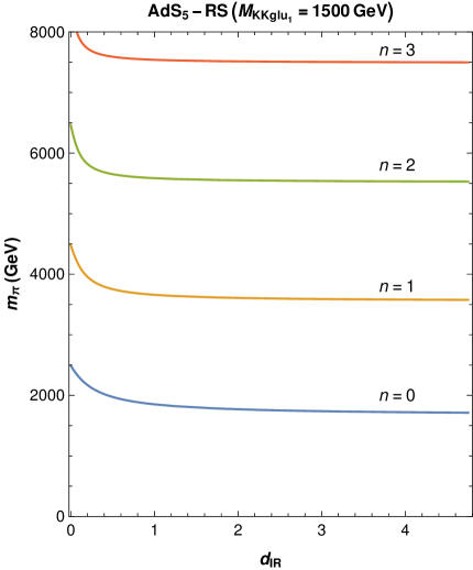
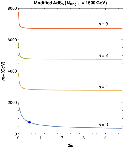
Figure 1: Mass spectrum of the first CP-odd Higgs scalars as a function of the brane kinetic term coefficient $d_{1}$ in the RS metric limit ($\nu=10$ and $y_{s}=4\ y_{1}$; left panel) and within a noticeably IR-modified $AdS_{5}$ metric ($\nu=0.5$ and $y_{s}=1.04\ y_{1}$; right panel). In both cases, the first KK gluon mass is fixed at 1500 GeV. One can see that in RS it is not possible to obtain a 750 GeV CP-odd scalar mass, whereas within the modified metric, a brane kinetic coefficient $d_{1}\simeq 0.51$ does produce a mass of 750 GeV, shown here as a dot.

In Fig. 1 we show the spectrum of the first 4 KK levels of CP-odd Higgs bosons $\Pi_{n}(x)$, for $n=0,1,2,3$, as a function of the brane kinetic term $d_{1}$ in units of the curvature $k\sim M_{Pl}$. The effects of the UV localized brane kinetic term are warped suppressed and so we do not consider them here anymore. We can see that in the RS limit, it is not possible to reduce sufficiently the lightest CP-odd mass to 750 GeV, as its mass tends asymptotically from about $2500$ GeV without brane kinetic term to about $1750$ GeV for large brane kinetic terms. On the other hand, with the modified metric it becomes possible to reduce greatly the lightest CP-odd mass with relatively small brane kinetic term coefficients (which in this particular case tends asymthotically to about 400 GeV). Parameter points such that the metric modification lies between the two considered will actually have an intermediate behavior, with a lightest CP-odd mass having increasing asymptotic values as one recovers the RS background.

Finally also note that the spectrum for the charged scalars is essentially the same since their differential equations and boundary conditions are identical except for the functions $M_{z}(y)$ and $M_{w}(y)$, which differ by about $10\%$. $M_{w}(y)$ produces a deviation from the CP-odd scalar spectrum of less than $5\%$. This means that the scenario under consideration should also contain a lightest charged Higgs scalar with a mass of about $750$ GeV also.

The next question to ask is how big is the effect of the Higgs brane kinetic term on the gauge bosons, and in particular on the lowest ones, i.e. the SM $W$ and $Z$ bosons. These terms represent an additional (brane localized) contribution to the mass of the gauge bosons. In principle their mass is generated here from a bulk Higgs mechanism, unless the brane kinetic terms are overly important (not the limit we are working with here). We can quickly estimate its effect on the lowest lying gauge fields. These are essentially flat (like all gauge zero modes) and thus their wave function is $f^{0}_{z}\sim 1/\sqrt{y_{1}}$. The contribution of a brane localized mass squared term is $\delta m^{2}_{z}\mathrel{\raise 1.29167pt\hbox{$<$\kern-7.5pt\lower 4.30554pt\hbox{$\sim$}}}d_{1}\ v^{2}/y_{1}\sim d_{1}\times 700$ GeV². For IR brane kinetic term coefficient $d_{1}$ of ${\cal O}(1)$, this represents naively at most some $10\%$ contribution to the overall mass squared of either $W$ or $Z$. In the particular case of the modified metric with a brane coefficient $d_{1}\simeq 0.51$, and metric parameters $\nu=0.5$ and $y_{s}=1.04\times y_{1}$ (which produces a light CP-odd scalar of $750$ GeV), the exact numerical effect on the zero mode gauge boson masses ($W$ and $Z$) is a shift of $3$ GeV with respect to the no-brane-kinetic-term limit. Of course, in the presence of brane kinetic terms, one redefines the VEV normalization constant, and the value of $g_{5}$, in order to correctly account for the SM gauge boson masses and electroweak couplings.

IV CP-odd Higgs couplings

As a $750$ GeV CP-odd Higgs scalar $\Pi_{0}(x)$ is allowed in the spectrum, thanks to the effect of small brane localized Higgs kinetic terms, we now study its couplings to SM particles in order to see if the observed excess at the LHC can be associated with this excitation. Of course being a CP-odd scalar its tree-level couplings to $ZZ$ and $WW$ are zero, making it an ideal candidate for the observed exotic events. We thus need to focus on its tree-level couplings to fermions (and top quark in particular), to $Zh$ (where $h$ is the $125$ GeV Higgs) and to its radiative couplings to photons and gluons. We study these in the subsequent subsections.

IV.1 Fermion couplings

The couplings of $\Pi_{0}(x)$ to fermions arise from two sources in the action. First source comes from the 5D Higgs Yukawa couplings, and second, from the gauge fermion couplings. This is because the physical field $\Pi_{0}(x)$ contains some of CP-odd Higgs scalar, and some of $Z_{5}$ excitation, where $Z_{5}$ is the fifth component of the 5D vector boson $Z_{M}$. However the 5D Yukawa coupling allows for direct coupling of $\Pi_{0}(x)$ to two zero-mode fermions, whereas the gauge-fermion coupling allows only couplings between fermion zero-modes and higher KK fermion levels. As we will see, it is important to keep both couplings, since after electroweak symmetry breaking the physical SM fermions (top quarks in particular) are mostly zero-modes but also contain a small amount of higher KK excitations, and could thus inherit some of the original gauge-fermion coupling, especially if the tree-level Yukawa coupling between $\Pi_{0}(x)$ and zero-mode top quarks is suppressed (as it can be).

The relevant terms in the action are the 5D Higgs Yukawa couplings and the fermion gauge interaction term,

$$S_{ff\Pi_{0}}\subset\int d^{4}xdy\sqrt{g}\left[Y_{u}HQU+Y_{d}HQD+h.c.+\bar{Q}{\cal D}/\ Q+\bar{U}{\cal D}/\ U+\bar{D}{\cal D}/\ D\right]$$ (21)

where $Q,U,D$ represent the 5D fermion $SU(2)_{L}$ doublets, up-type and down-type singlets (with generation indices and isospin indices suppressed). The kinetic terms contain the 5D covariant derivative and from them we extract the terms containing the CP-odd component $Z_{5}(x,y)$, and from the Higgs Yukawa couplings we extract the terms containing the CP-odd Higgs component $\Pi_{z}(x,y)$.

We follow the approach of Frank:2015zwd ; Diaz-Furlong:2016ril and compute these couplings by considering only the effects of three full KK levels, i.e. computing $21\times 21$ fermion Yukawa coupling matrices (with 3 $up$ and 3 $down$ families, each containing zero modes and 3 KK levels with an $SU(2)_{L}$ doublet and a singlet in each level, i.e., 3 zero modes plus $3\times 3\times 2$ KK modes). Note that we are interested in the couplings of the $750$ GeV CP-odd scalar $\Pi_{0}(x)$ to SM fermions (top quarks primarily), but we also need its couplings with the rest of KK fermions, since these interactions will be crucial to generate large enough radiative couplings to photons and gluons.

We first write the effective 4D up-type quark mass matrix as

$$\left(\begin{matrix}q^{0}_{L}(x)\ Q_{L}(x)\ U_{L}(x)\end{matrix}\right)\ M_{u}\ \left(\begin{matrix}u^{0}_{R}(x)\\ Q_{R}(x)\\ U_{R}(x)\end{matrix}\right)$$ (22)

in a basis where $q^{0}_{L}(x)$ and $u_{R}^{0}(x)$ represent three zero-mode flavors each (doublets and singlets of $SU(2)_{L}$), and $Q_{L}(x)$ and $Q_{R}(x)$ represent three flavors and three KK levels of the vector-like KK up-type doublets, and $U_{L}(x)$ and $U_{R}(x)$ represent three flavors and three KK levels of vector-like KK up-type singlets. The mass matrix is thus

$$M_{u}=\left(\begin{matrix}(y^{0}_{u})_{3\times 3}&(0)_{3\times 9}&(Y^{qU})_{3\times 9}\\ (Y^{Qu})_{9\times 3}&(M_{Q})_{9\times 9}&(Y_{1})_{9\times 9}\\ (0)_{9\times 3}&(Y_{2})_{9\times 9}&(M_{U})_{9\times 9}\end{matrix}\right)$$ (23)

with the down sector mass matrix ${M}_{d}$ computed in the same way.

The submatrices are obtained by evaluating the overlap integrals

$$y^{0}_{u}=\frac{(Y^{5D}_{u})_{ij}}{\sqrt{k}}\int_{0}^{y_{1}}dye^{-4\sigma(y)}\frac{v(y)}{\sqrt{2}}q^{0,i}_{L}(y)u^{0,j}_{R}(y)$$ (24)

$$Y^{qU}=\frac{(Y^{5D}_{u})_{ij}}{\sqrt{k}}\int_{0}^{y_{1}}dye^{-4\sigma(y)}\frac{v(y)}{\sqrt{2}}q^{0,i}_{L}(y)U^{n,j}_{R}(y)$$ (25)

$$Y^{Qu}=\frac{(Y^{5D}_{u})_{ij}}{\sqrt{k}}\int_{0}^{y_{1}}dye^{-4\sigma(y)}\frac{v(y)}{\sqrt{2}}Q^{m,i}_{L}(y)u^{0,j}_{R}(y)$$ (26)

$$Y_{1}=\frac{(Y^{5D}_{u})_{ij}}{\sqrt{k}}\int_{0}^{y_{1}}dye^{-4\sigma(y)}\frac{v(y)}{\sqrt{2}}Q^{m,i}_{L}(y)U^{n,j}_{R}(y)$$ (27)

$$Y_{2}=\frac{(Y^{5D^{*}}_{u})_{ij}}{\sqrt{k}}\int_{0}^{y_{1}}dye^{-4\sigma(y)}\frac{v(y)}{\sqrt{2}}Q^{m,i}_{R}(y)U^{n,j}_{L}(y)\,,$$ (28)

where the indices $m$ and $n$ track the KK level and $i,j=1,2,3$ are 5D flavor indices. The diagonal matrices $(M_{Q})_{9\times 9}$ and $(M_{U})_{9\times 9}$ are constructed with the masses of all the KK quarks involved. The masses and the profiles of the KK fermions appearing in these overlap integrals ($Q_{L}(y)$, $Q_{R}(y)$, $U_{L}(y)$ and $U_{R}(y)$) are obtained by solving differential equations for the fermion profiles

$$\partial_{y}\left(e^{(2c-1)\sigma(y)}\partial_{y}\left(e^{-(c+2)\sigma(y)}\right)\right)f(y)+e^{(c-1)\sigma(y)}m_{n}^{2}f(y)=0$$ (29)

where $f(y)$ is the KK profile. The mass eigenvalues $m_{n}$ are found by imposing Dirichlet boundary conditions on the wrong chirality modes.

As mentioned before, we have included 3 full KK levels so that the mass matrices in the gauge basis are $21\times 21$ dimensional matrices, which are not diagonal. One needs to diagonalize them, and by doing so, move to the quark physical basis where all the fermions couplings can then be extracted.

In the CP-odd scalar sector, we can write the effective 4D Yukawa-type couplings to fermions in the same gauge basis as before

$$\left(\begin{matrix}q^{0}_{L}(x)\ Q_{L}(x)\ U_{L}(x)\end{matrix}\right){\bf Y}_{\pi}\left(\begin{matrix}u^{0}_{R}(x)\\ Q_{R}(x)\\ U_{R}(x)\end{matrix}\right)\ \Pi_{0}(x)$$ (30)

where now the $21\times 21$ coupling matrix ${\bf Y}_{\pi}$ is given by

$${\bf Y}_{\pi}=\left(\begin{matrix}(y^{0}_{\pi qu})_{3\times 3}&(a_{\pi qQ})_{3\times 9}&(Y_{\pi qU})_{3\times 9}\\ (Y_{\pi Qu})_{9\times 3}&(a_{\pi QQ})_{9\times 9}&(Y_{1}^{\pi})_{9\times 9}\\ (a_{\pi uU})_{9\times 3}&(Y_{2}^{\pi})_{9\times 9}&(a_{\pi UU})_{9\times 9}\end{matrix}\right)$$ (31)

The submatrices are obtained by the overlap integrals

$$y^{0}_{\pi qu} = i\frac{(Y^{5D}_{u})_{ij}}{\sqrt{2k}}\int_{0}^{y_{1}}dye^{-3\sigma(y)}q^{0,i}_{L}(y)u^{0,j}_{R}(y)\frac{X_{\pi}^{\prime}(y)}{m^{2}_{\pi_{0}}M_{z}(y)}$$ (32)

$$Y_{\pi qU} = i\frac{(Y^{5D}_{u})_{ij}}{\sqrt{2k}}\int_{0}^{y_{1}}dye^{-3\sigma(y)}q^{0,i}_{L}(y)U^{n,j}_{R}(y)\frac{X_{\pi}^{\prime}(y)}{m^{2}_{\pi_{0}}M_{z}(y)}$$ (33)

$$Y_{\pi Qu} = i\frac{(Y^{5D}_{u})_{ij}}{\sqrt{2k}}\int_{0}^{y_{1}}dye^{-3\sigma(y)}Q^{m,i}_{L}(y)u^{0,j}_{R}(y)\frac{X_{\pi}^{\prime}(y)}{m^{2}_{\pi_{0}}M_{z}(y)}$$ (34)

$$Y^{\pi}_{1} = i\frac{(Y^{5D}_{u})_{ij}}{\sqrt{2k}}\int_{0}^{y_{1}}dye^{-3\sigma(y)}Q^{m,i}_{L}(y)U^{n,j}_{R}(y)\frac{X_{\pi}^{\prime}(y)}{m^{2}_{\pi_{0}}M_{z}(y)}$$ (35)

$$Y^{\pi}_{2} = i\frac{(Y^{5D^{*}}_{u})_{ij}}{\sqrt{2k}}\int_{0}^{y_{1}}dye^{-3\sigma(y)}Q^{m,i}_{R}(y)U^{n,j}_{L}(y)\frac{X_{\pi}^{\prime}(y)}{m^{2}_{\pi_{0}}M_{z}(y)}\,,$$ (36)

and

$$a_{\pi qQ} = \frac{g^{5D}_{L}}{\sqrt{k}}\int_{0}^{y_{1}}dye^{-2\sigma(y)}q^{0,i}_{L}(y)Q^{n,j}_{R}(y)\frac{X_{\pi}(y)}{m^{2}_{\pi_{0}}}$$ (37)

$$a_{\pi uU} = \frac{g^{5D}_{R}}{\sqrt{k}}\int_{0}^{y_{1}}dye^{-2\sigma(y)}u^{0,i}_{R}(y)U^{n,j}_{L}(y)\frac{X_{\pi}(y)}{m^{2}_{\pi_{0}}}$$ (38)

$$a_{\pi QQ} = \frac{g^{5D}_{L}}{\sqrt{k}}\int_{0}^{y_{1}}dye^{-2\sigma(y)}Q^{m,i}_{L}(y)Q^{n,j}_{R}(y)\frac{X_{\pi}(y)}{m^{2}_{\pi_{0}}}$$ (39)

$$a_{\pi UU} = \frac{g^{5D}_{R}}{\sqrt{k}}\int_{0}^{y_{1}}dye^{-2\sigma(y)}U^{m,i}_{R}(y)U^{n,j}_{L}(y)\frac{X_{\pi}(y)}{m^{2}_{\pi_{0}}}$$ (40)

where the $g^{5D}_{L,R}$ coupling are given by

$$g^{5D}_{L}={g^{5D}\over\cos\theta_{W}}\left(T_{3}-Q_{q}\sin^{2}\theta_{W}\right)$$ (41)

$$g^{5D}_{R}={g^{5D}\over\cos\theta_{W}}Q_{q}\sin^{2}\theta_{W},$$ (42)

with $Q_{q}$ the charge of the quark, (here ${2\over 3}$), $\theta_{W}$ the weak angle and $T_{3}={1\over 2}$. Note that when the interaction originates in the 5D Yukawa couplings, the profile to use is the one coming from the CP-odd Higgs component, i.e proportional to $X_{\pi}^{\prime}(y)$. When the interaction originates in the gauge fermion coupling and thus comes from the $Z_{5}$ component, the profile to use is proportional to $X_{\pi}(y)$, with $X_{\pi}$ being the solution of Eq. (18), using the decompositions of Eqs. (14) and (15).

When the fermion matrix in (23) is diagonalized, the coupling matrix of fermions with the CP-odd field $\Pi_{0}(x)$ in (31) is rotated, and we can then extract all the physical Yukawa couplings. All these couplings are needed later in order to compute the radiative couplings of $\Pi_{0}(x)$ with gluons and photons.

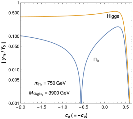
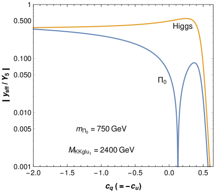
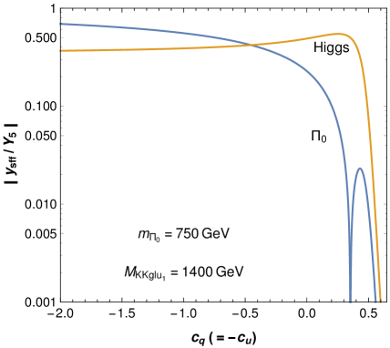
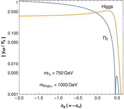
Figure 2: Yukawa couplings between zero-mode fermions and the two lightest neutral scalars of the scenario, the $125$ GeV Higgs and the $750$ GeV CP-odd $\Pi_{0}$. The couplings are evaluated relative to the 5D bulk Higgs Yukawa coupling $Y_{5}$ and are shown as a function of the fermion bulk mass parameter $c_{q}$ (in the case $c_{q}=-c_{u}$ for simplicity) for different overall KK scales, $M_{KKglu_{1}}=3900$ GeV (upper left panel), $M_{KKglu_{1}}=2400$ GeV (upper right panel), $M_{KKglu_{1}}=1400$ GeV (lower left panel) and $M_{KKglu_{1}}=1000$ GeV (lower right panel). The CP-odd scalar mass is set to $750$ GeV and for certain values of $c_{q}$ its Yukawa coupling to top quarks can be highly suppressed for typical top-quark values of the $c_{i}$’s.

We first analyze the very important Yukawa coupling between $\Pi_{0}(x)$ and top quarks, as this coupling might dominate the decays of the CP-odd scalar. This coupling comes essentially from the entry $(y^{0}_{\pi qu})_{33}$ (before rotation to the physical basis) although it receives small corrections after going to the physical basis. We focus on $(y^{0}_{\pi qu})_{33}$ which comes from the overlap integral

$$(y^{0}_{\pi qu})_{33} = i\frac{(Y^{5D}_{u})_{33}}{\sqrt{2k}}\int_{0}^{y_{1}}dye^{-3\sigma(y)}q^{0}_{t}(y)u^{0}_{t}(y)\frac{X_{\pi}^{\prime}(y)}{m^{2}_{\pi_{0}}M_{z}(y)}$$ (43)

In the RS limit, the warp factor is $\sigma(y)=ky$, and the top profiles are $q^{0}_{t}(y)=f(c_{q})e^{(2-c_{q})ky}$ and $u^{0}_{t}(y)=f(-c_{u})e^{(2+c_{u})ky}$, where $f(x)$ is a normalization factor. We also have $M_{z}(y)=\frac{g_{5}}{2c_{W}}v_{0}e^{(a-1)ky}$, with $v_{0}$ a constant factor, so that the previous overlap integral in this limit reads

$$(y^{0}_{\pi qu})_{33}=i\frac{(Y^{5D}_{u})_{33}}{\sqrt{2k}}\frac{2c_{W}}{g_{5}}\frac{f(c_{q})f(-c_{u})}{v_{0}m^{2}_{\pi_{0}}}\int_{0}^{y_{1}}dy\ e^{(2-a-c_{q}+c_{u})ky}X_{\pi}^{\prime}(y)$$ (44)

We integrate this by parts to find

$$\!\!\!(y^{0}_{\pi qu})_{33} = -i\frac{(Y^{5D}_{u})_{33}}{\sqrt{2k}}\frac{2c_{W}}{g_{5}}\frac{f(c_{q})f(-c_{u})}{v_{0}m^{2}_{\pi_{0}}}\int_{0}^{y_{1}}dy\ (2-a-c_{q}+c_{u})e^{(2-a-c_{q}+c_{u})ky}X_{\pi}(y)+BT\ \ \ \ \ \$$ (45)

where $BT=i\frac{(Y^{5D}_{u})_{33}}{\sqrt{2k}}\frac{2c_{W}}{g_{5}}\frac{f(c_{q})f(-c_{u})}{v_{0}m^{2}_{\pi_{0}}}\ e^{(2-a-c_{q}+c_{u})ky}X_{\pi}(y)\Big{|}_{0}^{y_{1}}$ is a boundary term. Note that the profile $X_{\pi}(y)$ has vanishing boundary conditions in the absence of Higgs localized brane kinetic terms. In that limit we can see that the coupling of the CP-odd scalar can actually vanish, when $(2-a-c_{q}+c_{u})=0$ Archer:2012qa . Note also that the Higgs localizer parameter $a$ is, in this RS limit, $a\mathrel{\raise 1.29167pt\hbox{$>$\kern-7.5pt\lower 4.30554pt\hbox{$\sim$}}}2$ and the bulk parameters $c_{q}$ and $c_{u}$ are defined such that, for example, charm or bottom quarks are assigned values more or less $c_{q}\in(0.45,0.55)$ and $c_{u}\in(-0.5,-0.6)$, whereas for top we have $c_{q_{3}}\sim 0.45$ and $c_{u_{3}}>-0.45$. This means that we expect the term $(2-a-c_{q}+c_{u})$ to vanish, in the limit of $a\sim 2$, when $c_{q}-c_{u}\sim 0$, so that the suppression in this case seems only possible for the top quark, where both $c_{q}$ and $c_{u}$ could be small.

Of course when the metric background is modified, and the boundary conditions include the brane kinetic terms there will be deviations from the previous values. Nevertheless it is clear that the Yukawa coupling of the CP-odd scalar field to top quarks can have highly suppressed values. Another way to see this is to consider the overlap integral in Eq. (43). Because the profile $X_{\pi}(y)$ vanishes at the boundaries (or $almost$ vanishes, for small brane kinetic terms), then its derivative $X^{\prime}_{\pi}(y)$ will have a node in the bulk, and therefore will change sign. That means that there can be some parameter choice for which it is possible for the overlap integral to vanish, since the fermion zero mode profiles have no nodes in the bulk.

This feature is clearly seen in Fig. 2, where we plot the absolute value of the Yukawa couplings between zero-mode fermions and both the Higgs and the CP-odd scalar $\Pi_{0}(x)$. The couplings shown are relative to the 5D bulk Higgs Yukawa coupling $Y_{5}$ and are plotted as functions of the fermion bulk mass parameter $c_{q}$ and $c_{u}$ (for the case where we take $c_{q}=-c_{u}$, for simplicity), for different overall KK scales. We observe that the CP-odd Yukawa couplings are fairly similar to the Higgs Yukawa couplings (i.e. exponentially sensitive to UV localization and then top-like when the zero mode is IR localized) except that there is a range of parameters where the coupling vanishes. Interestingly enough, this suppression happens for preferred values of the top quark bulk mass parameters. This means that the existence of suppressed couplings to top quarks of the CP-odd $\Pi_{0}$ is a natural possibility in this scenario.

IV.2 Radiative couplings to photons and gluons

Just like in the Higgs boson case, the radiative couplings of $\Pi_{0}(x)$ to gluons and photons will depend on the physical Yukawa couplings $y_{nn}$ between $\Pi_{0}$ and the fermions (zero modes and KK modes) running in the loop, as well as on the fermion masses $m_{n}$ (the eigenvalues of the mass matrix in Eq.(23)). The real and imaginary parts of the couplings are associated with different loop functions, $A^{S}_{1/2}$ and $A^{P}_{1/2}$, as they generate the two operators $\Pi_{0}G_{\mu\nu}G^{\mu\nu}$ and $\Pi_{0}G_{\mu\nu}\tilde{G}^{\mu\nu}$.

The production cross section through gluon fusion is

$$\sigma_{gg\rightarrow\Pi_{0}}={\alpha_{s}^{2}m_{\Pi_{0}}^{2}\over 576\pi}\left[\Big{|}\sum_{quarks}c^{S}_{n}\Big{|}^{2}+\Big{|}\sum_{quarks}c^{P}_{n}\Big{|}^{2}\right]\$$ (46)

and the decay widths to gluons and photons are

$$\Gamma_{\Pi_{0}\to gg}=\frac{\alpha_{s}^{2}m^{3}_{\Pi_{0}}}{54\pi^{2}}\frac{1}{v^{2}}\left[\Big{|}\sum_{{quarks}}c^{S}_{n}\Big{|}^{2}+\Big{|}\sum_{{quarks}}c^{P}_{n}\Big{|}^{2}\right]\$$ (47)

$$\Gamma_{\Pi_{0}\to\gamma\gamma}=\frac{\alpha^{2}m^{3}_{\Pi_{0}}}{192\pi^{3}}\frac{1}{v^{2}}\left[\Big{|}\sum_{{quarks\atop leptons}}N_{c}Q_{n}^{2}c^{S}_{n}\Big{|}^{2}+\Big{|}\sum_{{quarks\atop leptons}}N_{c}Q_{n}^{2}c^{P}_{n}\Big{|}^{2}\right]\$$ (48)

where $\alpha_{s}$ and $\alpha$ are the strong and weak coupling constants, $N_{c}$ is the number of colors and $Q_{n}$ is the charge of the fermion, and where

$$c^{S}_{n}=\hbox{Re}\left({\frac{y_{nn}}{m_{n}}}\right)A^{S}_{1/2}(\tau_{n})\hskip 17.07182pt{\rm and}\hskip 17.07182ptc^{P}_{n}={\rm Im}\left(\frac{y_{nn}}{m_{n}}\right)A^{P}_{1/2}(\tau_{n})$$ (49)

with $\ \tau_{n}=m^{2}_{\Pi_{0}}/4m^{2}_{n}\$ and with the loop functions defined as Gunion:1989we

$$A^{S}_{1/2}(\tau) = {3\over 2}\left[\tau+(\tau-1)f(\tau)\right]\tau^{-2},$$ (50)

$$A^{P}_{1/2}(\tau) = -{3\over 2}f(\tau)/\tau,$$ (51)

and with

$$f(\tau)=\left\{\begin{tabular}[]{cc}$\left[\arcsin\sqrt{\tau}\right]^{2}$&$(\tau\leq 1)$\\ $-{1\over 4}\left[\ln\left({1+\sqrt{1-\tau^{-1}}\over 1-\sqrt{1-\tau^{-1}}}\right)-i\pi\right]^{2}$&$(\tau>1)$ .\end{tabular}\right.$$ (54)

For heavy KK quarks with masses $m_{n}$ much greater than the CP-odd mass $m_{\Pi_{0}}$ (i.e. when $\tau$ is very small) the loop functions are essentially constant, as they behave asymptotically as $\displaystyle\lim_{\tau\to 0}A^{S}_{1/2}=1\hskip 5.69046pt\mbox{and}\hskip 5.69046pt\lim_{\tau\to 0}A^{P}_{1/2}=3/2.$ On the other hand, for light quarks (all the SM quarks except top and bottom), the loop functions essentially vanish asymptotically as $\displaystyle\lim_{\tau\to\infty}A^{S}_{1/2}=\lim_{\tau\to\infty}A^{P}_{1/2}=0.$

Moreover, we investigate a parameter region where the couplings of $\Pi_{0}$ to top quarks are highly suppressed. This means that the production mechanism must rely exclusively on the heavy KK fermions running in the loop and as we have seen, this coupling depends on the ratio $\frac{y_{nn}}{m_{n}}$ between the physical Yukawa coupling and the mass of the fermion running in the loop. To have an idea of the relative contribution of each of these KK fermions in the loop, in Fig. 3 we plot the mass normalized Yukawa couplings of Standard Model Higgs with top quarks, Higgs with first KK fermion and of $\Pi_{0}$ to first KK fermion, for different values of the KK scale. As expected we see that the $c_{q}$ dependence is mild (i.e. all KK fermions of any flavor will couple with similar strength) and also, as expected, we observe that the mass normalized couplings are quite suppressed with respect to the SM top quark case. Still the multiplicity of KK fermions is high, since there are 6 families of quarks and 3 families of charged leptons (the latter run in the diphoton loop), and for each family there are a few KK levels that give important contributions to the rate.

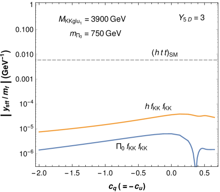
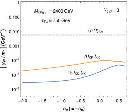
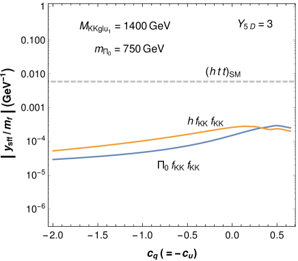
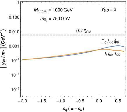
Figure 3: Yukawa couplings between the lightest KK fermion and the $125$ GeV Higgs (middle curves) and the $750$ GeV CP-odd $\Pi_{0}$ (lower curves), divided by the KK fermion mass, for different values of the lightest KK gluon mass $M_{KKglu_{1}}$, as indicated on the panels. This mass normalized Yukawa coupling gives an estimate of the relative contribution of the respective KK fermion to the radiative coupling of the scalar to gluons and photons, to be compared with the mass normalized SM coupling of Higgs to top quarks (shown as a dashed line).

A numerical scan of the couplings, including all families and 3 full KK levels is computationally too intensive, so in order to produce the couplings plotted in Fig. 3 we performed an approximation, sufficient for the purposes of the graph.

The KK fermion Yukawa couplings plotted neglect mixings between different KK levels and different flavors, and with the zero mode fermions. They are obtained as follows. Consider the $2\times 2$ KK mass matrix

$$\left(\begin{matrix}Q_{L}(x)\ U_{L}(x)\end{matrix}\right)\ M_{u}\ \left(\begin{matrix}Q_{R}(x)\\ U_{R}(x)\end{matrix}\right),$$ (55)

where $Q_{L}(x)$ and $Q_{R}(x)$ represent here a single flavor and a single KK level of the vector-like KK up-type doublets, and similarly for $U_{L}(x)$ and $U_{R}(x)$, vector-like KK up-type singlets. The mass matrix is thus

$$M_{u}=\left(\begin{matrix}m_{Q}&Y_{1}\\ Y_{2}&m_{U}\end{matrix}\right),$$ (56)

where the diagonal entries are the KK masses (large) whereas the off-diagonal entries are coming from Yukawa couplings and are therefore smaller. In order to give a simple estimate, we take for simplicity the fermion bulk mass parameters as $c_{q}=-c_{u}$, and the bulk Higgs Yukawa $Y^{5D}$ to be real, which leads to $Y_{1}=Y_{2}$ and $m_{Q}=m_{U}=m_{KK}$, with the masses and profiles obtained by solving Eq. (29). With the KK fermion profiles one obtains the off-diagonal entries

$$Y_{1}=\frac{(Y^{5D}_{u})}{\sqrt{k}}\int_{0}^{y_{1}}dye^{-4\sigma(y)}\frac{v(y)}{\sqrt{2}}Q_{L}(y)U_{R}(y).$$ (57)

The matrix that diagonalizes (56) in this simple limit ($c_{q}=-c_{u}$) is $\left(\begin{matrix}-\frac{1}{\sqrt{2}}&\frac{1}{\sqrt{2}}\\ \frac{1}{\sqrt{2}}&\frac{1}{\sqrt{2}}\end{matrix}\right)$ and the eigenvalues are $m_{1}=m_{KK}-Y_{1}$ and $m_{2}=m_{KK}+Y_{1}$.

Now we apply this rotation to the CP-odd Yukawa coupling matrix

$$Y_{\Pi}=\left(\begin{matrix}{\cal O}(g)&Y_{\pi}\\ Y_{\pi}&{\cal O}(g)\end{matrix}\right),$$ (58)

where

$$Y_{\pi} = i\frac{(Y^{5D}_{u})_{ij}}{\sqrt{2k}}\int_{0}^{y_{1}}dye^{-3\sigma(y)}Q_{L}(y)U_{R}(y)\frac{X_{\pi}^{\prime}(y)}{m^{2}_{\pi_{0}}M_{z}(y)},$$ (59)

and where for simplicity we have neglected gauge couplings terms compared to IR Yukawa terms (safe assumption when $Y^{5D}$ is large).

After diagonalization, we obtain the two physical couplings between $\Pi_{0}$ and the KK fermions. When we normalize the couplings by the two eigenmasses and add the two contributions, we obtain

$$\sum_{i=1}^{2}\frac{y_{i}}{m_{i}}=\frac{y_{1}^{\pi}}{m_{1}}+\frac{y_{2}^{\pi}}{m_{2}}=-2\frac{Y_{1}Y_{\pi}}{m_{KK}^{2}-Y_{1}^{2}}\simeq-2\frac{Y_{1}Y_{\pi}}{m_{KK}^{2}}.$$ (60)

The last expression corresponds to the mass normalized Yukawa couplings of $\Pi_{0}$ plotted in Fig. 3, and this describes very closely the behavior of the couplings obtained in the full flavor calculation. The parametric dependence of these couplings is $Y_{5D}^{2}v/m_{KK}^{2}$, so that if $Y^{5D}\sim 3$ we expect mass normalized couplings of order $(10^{-3}-10^{-4})$ GeV^-1, if the overlap integral is of ${\cal O}(1)$. Since all the profiles of the integral are IR localized, one expects that integral to be ${\cal O}(1)$, although the precise numerical result varies between $0.5$ and $0.05$, depending on the values of the $c_{q}$ parameter, as shown in the plots.

All in all it seems likely that after taking into consideration all the fermion flavors, and for a KK scale of order $1-2$ TeV, the overall KK fermion contribution to the radiative couplings of $\Pi_{0}(x)$ to photons and gluons can be close to the top quark contribution to the gluon and photon couplings of the Higgs in the SM model.

IV.3 $\Pi_{0}Zh$ coupling

The coupling between the CP-odd scalar, the $Z$ boson and the Higgs will be extracted from the kinetic operator of the 5D Higgs,

$$\int d^{4}xdy\ e^{-2\sigma}D_{\mu}H^{\dagger}D^{\mu}H\left(1+\delta(y-y_{i})\frac{d_{i}}{k}\right).$$ (61)

Expanding the SM-like Higgs mode using Eq. (5) as well as the SM-like $Z_{\mu}$ and the $750$ GeV $\Pi_{0}$ using Eqs. (6) and (7), we can obtain the coefficient $g_{\Pi hZ}$ of the operator $Z^{\mu}(x)\Big{(}h(x)\partial_{\mu}\Pi_{0}(x)+\Pi_{0}(x)\partial_{\mu}h(x)\Big{)}$

$$g_{\Pi hZ}=\frac{g_{5}^{2}}{4c_{W}^{2}}\int dye^{-2\sigma}v(y)h(y)f_{z}(y)\frac{X^{\prime}(y)}{M^{2}_{z}(y)m^{2}_{\pi}}\left(1+\delta(y-y_{i})\frac{d_{i}}{k}\right)$$ (62)

Now since $M_{z}(y)=\frac{g_{5}}{2c_{W}}e^{-\sigma}v(y)$, $h(y)\sim v(y)/v_{4}$, and $f_{z}\simeq 1/\sqrt{y_{1}}$ we can write

$$g_{\Pi hZ}\simeq\frac{1}{\sqrt{y_{1}}v_{4}m^{2}_{\pi}}\big{(}X(y_{1})+X^{\prime}(y_{1})\frac{d_{1}}{k}\big{)}=0,$$ (63)

where we have used the boundary conditions for the profile $X(y)$ (see Eq.(19)) and assumed no UV brane kinetic term ($d_{0}=0$).

The coupling should thus vanish in the limit of flat $Z$ boson profile $f_{z}(y)$, and when the nontrivial Higgs VEV $v(y)$ is proportional to the Higgs scalar profile $h(y)$. Corrections to these limits scale as $v_{4}^{2}/m_{KK}^{2}$ and $m_{h}^{2}/m_{KK}^{2}$ in the RS case, and so we expect the overall coupling to be highly suppressed.

The partial width for the decay $\Pi_{0}\to hZ$ is djouadi1996

$$\Gamma(\Pi_{0}\to hZ)=\frac{g^{2}_{\Pi hZ}}{16\pi}\frac{m_{Z}^{2}}{m_{\pi}}\sqrt{\lambda(m^{2}_{h},m^{2}_{Z};m^{2}_{\pi})}\lambda(m^{2}_{h},m^{2}_{\pi};m^{2}_{Z})$$ (64)

where $m_{Z}$, $m_{\pi}$ and $m_{h}$ are the masses of the particles involved and where $\lambda(x,y;z)=(1-x/z-y/z)^{2}-4xy/z^{2}$. With the masses $m_{Z}=91$ GeV, $m_{\pi}=750$ GeV and $m_{h}=125$ GeV, the width becomes $\Gamma(\Pi_{0}\to hZ)\sim(900\ g^{2}_{\Pi hZ})$ GeV.

For example we compute numerically $g_{\Pi hZ}$ for three different values of $M_{KKglu_{1}}$, and with $m_{\Pi_{0}}=750$ GeV and find

$M_{KKglu_{1}}$	1000 GeV	1400 GeV	2400 GeV
$g_{\Pi hZ}$	$3.8\times 10^{-4}$	$3.1\times 10^{-3}$	$1.1\times 10^{-2}$
$\Gamma(\Pi_{0}\to hZ$)	$1.3\times 10^{-4}$ GeV	$8.8\times 10^{-3}$ GeV	$0.11$ GeV

Note that the couplings and widths are small but we observe that the partial width becomes larger as the KK mass scale is increased. Since we need the partial width $\Gamma(\Pi_{0}\to\gamma\gamma)$ to be similar to that of a $750$ GeV Higgs, i.e. $\Gamma(h_{750GeV}\to\gamma\gamma)\sim 10^{-5}$ GeV, we expect that at $M_{KKglu_{1}}=1400$ GeV the $Zh$ signal should start putting too much pressure on the allowed parameter space. This is confirmed in the full numerical analysis presented in the next section.

IV.4 Estimates and numerical results

With all the previous ingredients one can estimate the viability of this scenario in terms of the possible diphoton excess. Let’s choose the KK scale such that $M_{KKglu_{1}}=1400$ GeV; when the bulk mass parameters of the top quark are around $|c_{u_{3}}|\sim 0.35$ we know that the top quark will have highly suppressed couplings to $\Pi_{0}$, as shown in the third panel of Fig. 2 . At the same time, the couplings of the KK tops (as well as all other KK quarks) will have relatively strong Yukawa couplings to $\Pi_{0}$ (third panel of Fig. 3), so that the contribution of each of them to the radiative coupling of $\Pi_{0}$ to gluons is about an order of magnitude smaller than the top contribution to the $h-glu-glu$ coupling of the SM. Thus we could estimate that the overall contribution of all flavors and KK excitations can make up for the suppressed coupling, so that the production cross section of $\Pi_{0}$ is similar to that of a $750$ GeV SM-like Higgs.

The production cross section of a $750$ GeV Higgs through gluon fusion, at the LHC running at 13 TeV is $497$ fb Dittmaier:2011ti , so, roughly, this could be assumed for the $\Pi_{0}$ production cross section.

Since the $\Pi_{0}$ decays to top quarks and $hZ$ are suppressed in this parameters space point, and its decays to $WW$ and $ZZ$ can only be radiative via the CP-odd gauge boson kinetic operator, the main decay channel is into gluons so that the branching of the diphoton channel should be very roughly

$$Br(\Pi_{0}\to\gamma\gamma)\sim\frac{\alpha^{2}_{em}}{8\alpha^{2}_{s}}\frac{N_{\gamma}}{N_{glu}}$$ (65)

where $N_{\gamma}$ and $N_{glu}$ are the multiplicities of states running in the $(\Pi_{0}\gamma\gamma)$ loop and in the $(\Pi_{0}\ glu\ glu)$ loop respectively.

In the diphoton loop there are $3$ extra families of charged lepton KK excitations making the multiplicity of states greater. If their multiplicity and their Yukawa couplings can partially make up for the color factor of 8, then the diphoton cross section might become of ${\cal O}$ (1 fb), as hinted by the December 2015 LHC data.

To complete the analysis, we perform a full numerical computation of production and branching ratios in a setup where we consider an effective 4D scenario including three full KK levels for all fields, i.e., we consider $21\times 21$ fermion mass matrices, which we diagonalize in order to obtain the physical Yukawa couplings. We choose a set of $c$-parameters and 5D Yukawa entries such that the SM masses and mixings are reproduced; the specific flavor choice for these parameters should not affect much the overall results since these depend on overlap integrals between IR localized fields, with very loose $c$-dependence. We choose the background metric parameters so that precision electroweak bounds are kept at bay, i.e. $\nu=0.5$ and $y_{s}=1.04y_{1}$. Two average 5D Yukawa scales are considered, $Y_{5D}\simeq 3$ and $Y_{5D}\simeq 2$, to show the dependence on this parameter, and we also consider two different KK mass scales, $M_{KKglu_{1}}=1000$ GeV and $M_{KKglu_{1}}=1300$ GeV, which turn out to lead to successful signal generation.

In order to see how tuned is the choice of top $c$-parameter, we plot the production cross section of the CP odd resonance, followed by decays into $\gamma\gamma$, $t\bar{t}$ and $Zh$, as functions of $c_{u_{3}}$ (the bulk mass parameter of the 5D singlet top quark), with the doublet bulk mass parameter fixed at $c_{q_{3}}=0.4$. (This value ensures typically suppressed bounds from $Zb_{L}{\bar{b}}_{L}$ bounds Cabrer ).

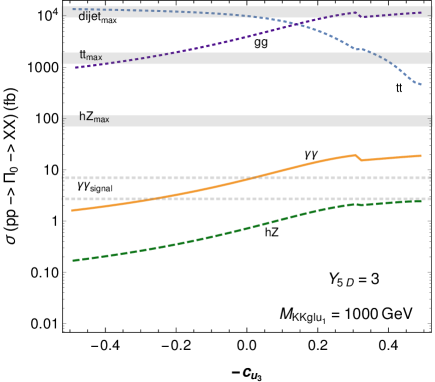
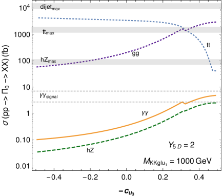
Figure 4: Production cross sections at the LHC running at 13 TeV in the channels $\gamma\gamma$, $t\bar{t}$ and $hZ$. The lightest KK boson mass is $1000$ GeV and the 5D Yukawa couplings are $Y_{5D}\simeq 3$ in the left panel and $Y_{5D}\simeq 2$ in the right panel. The signal can always be produced at this KK scale but for larger 5D Yukawa couplings there are either too many top pairs or too many dijets produced. Overall we can conclude that for $M_{KKglu_{1}}=1000$ GeV and when $1\mathrel{\raise 1.29167pt\hbox{$<$\kern-7.5pt\lower 4.30554pt\hbox{$\sim$}}}Y_{5D}\mathrel{\raise 1.29167pt\hbox{$<$\kern-7.5pt\lower 4.30554pt\hbox{$\sim$}}}3$ and $0.2\mathrel{\raise 1.29167pt\hbox{$<$\kern-7.5pt\lower 4.30554pt\hbox{$\sim$}}}|c_{u_{3}}|\mathrel{\raise 1.29167pt\hbox{$<$\kern-7.5pt\lower 4.30554pt\hbox{$\sim$}}}0.5$ the signal is easily reproduced.

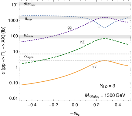
Figure 5: Same as the previous figure but for a KK scale of $1300$ GeV. In this case the signal can only be achieved for larger Yukawa couplings, and at a more localized region near $c_{u_{3}}\sim 0.25$. The bound from $hZ$ now becomes the main constrain. For heavier KK mass scales, the signal can only be produced for much larger Yukawa couplings and the $hZ$ bound becomes too constraining.

The results are shown in Figs. 4 and 5, where we have chosen two KK scales, $M_{KKglu_{1}}=1000$ GeV and $M_{KKglu_{1}}=1300$ GeV. In both cases we show results for $Y_{5D}\simeq 3$ and $Y_{5D}\simeq 2$ to illustrate the sensitivity on this bulk parameter, crucial for enhancing the radiative couplings of $\Pi_{0}$. When the KK scale is smaller and 5D Yukawa couplings are larger, the production of top pairs and gluon pairs can be too large. By reducing the 5D Yukawa couplings, enough signal can be generated with the dijets and top pairs under control, as well as the $Zh$ decay. The values of $|c_{u_{3}}|$ must be in the region $0.2\mathrel{\raise 1.29167pt\hbox{$<$\kern-7.5pt\lower 4.30554pt\hbox{$\sim$}}}|c_{u_{3}}|\mathrel{\raise 1.29167pt\hbox{$<$\kern-7.5pt\lower 4.30554pt\hbox{$\sim$}}}0.5$. For slightly smaller KK scales one expects a similar behavior, but such that 5D Yukawa couplings should be smaller in order to suppress overproduction of $\Pi_{0}$ particles.

This leads to the question of how large can the KK scale be and still manage to produce enough signal. We observe that at $M_{KKglu_{1}}=1300$ GeV, larger 5D Yukawa couplings ($Y_{5d}\geq 3$) are required in order to have enough signal production. The branching fraction into $hZ$ starts to be problematic, and actually becomes worse for heavier KK scales. The signal production requires that the value of $|c_{u_{3}}|$ be located around the point where the top Yukawa couplings of $\Pi_{0}$ are suppressed, in this case around $|c_{u_{3}}|\sim 0.3$.

We conclude therefore that in order to explain the $750$ GeV diphoton, the KK scale must be $M_{KKglu_{1}}\leq 1300$ GeV, with 5D Yukawa couplings $Y_{5D}\mathrel{\raise 1.29167pt\hbox{$<$\kern-7.5pt\lower 4.30554pt\hbox{$\sim$}}}3$. For those values, the signal is quite generic (i.e. small, but typical, $c_{u_{3}}$ values are required), as long as the $\Pi_{0}$ mass is set to $750$ GeV with appropriate boundary kinetic terms.

V Discussion

We performed an analysis of the scalar sector of warped space models to investigate whether the minimal model can accommodate a resonance at 750 GeV with the properties observed in the diphoton resonance at the CMS and ATLAS. We show that in the simplest extra dimensional extension of the SM, that is with a 5D Higgs doublet living in the bulk, the lowest pseudoscalar KK excitation can be responsible for the signal observed at 750 GeV. We emphasize that, unlike other explanations relying on scalar fields in warped models, ours does not introduce any new fields or representations, but relies on Higgs brane kinetic terms to lower the KK mass of the lightest CP odd Higgs resonance. This makes the model extremely constrained, with the only new parameter being the IR brane kinetic coefficient $d_{1}$. The lightest CP odd excitation, a mixture of the 5D Higgs field and $Z_{5}$, does not decay at tree level into $WW$ or $ZZ$, and, over a range of the parameter space, can have suppressed couplings to the top quark, thus a small decay width into $t{\bar{t}}$. The production through gluon fusion can be loop-enhanced through the effects of the usual KK fermion modes, and so can the diphoton decay. The coupling to $Zh$ is also suppressed although starts increasing dangerously for KK masses above $1500$ GeV.

We also showed that in $AdS_{5}$ spaces (RS-type models) with a KK scale as low as $1500$ GeV, the lowest CP-odd scalar cannot have a mass at 750 GeV, but if the metric differs slightly from the $AdS_{5}$ metric (generalized warped metric spaces), the Higgs brane kinetic terms can produce a viable CP-odd scalar of mass 750 GeV.

Within these modified metric scenarios, and for KK mass scales at around 1 TeV (consistent with precision electroweak bounds) this CP odd resonance obeys the (current) experimental constraints. We analyzed its production and decay for several values of the lowest KK gluon mass ($M_{KKglu_{1}}$), and show that consistency with the data requires $M_{KKglu_{1}}\mathrel{\raise 1.29167pt\hbox{$<$\kern-7.5pt\lower 4.30554pt\hbox{$\sim$}}}1300$ GeV.

Our analysis is quite general, and should be valid even in the absence of a signal at 750 GeV. The general conclusion to be taken from our analysis here is that warped space models, without any new particles, can explain a (relatively) light diphoton resonance at the LHC. Should a diphoton excess be found at higher values, even the RS model might accommodate such a state without the need modify the metric.

Among the general features of the light CP-odd scalar resonance, resulting from the 5D Higgs doublet are the fact that its coupling to top pairs can be suppressed for appropriate top bulk mass parameters. Also its coupling to $Zh$ is generically suppressed due to the boundary conditions of the CP odd state. In addition, the model predicts that the spectrum for the CP odd and the charged scalars is essentially the same since their differential equations and boundary conditions are almost identical. This means that the lightest charged Higgs boson is expected to have a mass very close to the pseudoscalar mass, so about 750 GeV, in the scenario in which the latter is the diphoton resonance.

If the diphoton resonance ends up being a real particle, and not a statistical fluctuation, the prediction from this scenario is that $ZZ$ and $WW$ should not be seen, whereas top pair production, dijet production and $Zh$ signal should be around the corner. Moreover a search for the charged scalars at around $750$ GeV might prove useful in order to disentangle the different models explaining the resonance.

VI Acknowledgments

MF and MT thank NSERC and FRQNT for partial financial support under grant numbers SAP105354 and PRCC-191578.

VII Appendix

In this section we consider the effect of brane localized kinetic terms associated with the 5D Higgs doublet and also with the gauge bosons. For simplicity, let’s consider a 5D toy model with a Higgs scalar $H(x,y)$ charged under a local $U(1)$, defined by the following action:

$$S = \int d^{4}xdy\sqrt{g}\ \left(-\frac{1}{4}F^{2}_{MN}+|D^{M}H|^{2}-V(H)\right)$$ (67)

$$\ \ \ +\sum_{i}\int d^{4}xdy\sqrt{g}\ \delta(y-y_{i})\left(\frac{1}{4}r_{i}F^{2}_{MN}+d_{i}|D^{M}H|^{2}-\lambda_{i}(H))\right)$$

where $F_{MN}=\partial_{M}A_{N}-\partial_{N}A_{M}$ and for simplicity we set gauge coupling constant to unity in the appropriate mass dimensions. The background spacetime metric is assumed to take the form

$$ds^{2}=e^{-2\sigma(y)}\eta_{\mu\nu}dx^{\mu}dx^{\nu}-dy^{2}$$ (68)

where $\sigma(y)$ is the warp factor.

We are interested in studying the effective 4D perturbative spectrum of the 5D Higgs field and the 5D gauge boson, around a nontrivial Higgs vacuum profile solution $<H>=v(y)$.

$$H(x,y)=\frac{1}{\sqrt{2}}\left(v(y)+h(x,y)\right)e^{i\pi(x,y)}$$ (69)

In particular we are interested in the CP-odd Higgs perturbations $\pi(x,y)$, whose equations of motion are coupled with the gauge boson perturbations. The equations read

$$(1+r_{i}\delta_{i})\partial_{\mu}\partial^{\mu}A_{\mu}-\left((1+r_{i}\delta_{i})e^{-2\sigma}A^{\prime}_{\mu}\right)^{\prime}+(1+d_{i}\delta_{i})M_{A}^{2}A_{\mu}+$$

$$\hskip 85.35826pt\partial_{\mu}\left((1+d_{i}\delta_{i})M_{A}^{2}\pi-(1+r_{i}\delta_{i})\partial^{\nu}A_{\nu}-\left((1+r_{i}\delta_{i})e^{-2\sigma}A_{5}\right)^{\prime}\right)=0$$ (70)

$$(1+r_{i}\delta_{i})\partial_{\mu}\partial^{\mu}A_{5}-(1+r_{i}\delta_{i})\partial^{\nu}A^{\prime}_{\nu}+(1+d_{i}\delta_{i})M_{A}^{2}(\pi^{\prime}-A_{5})=0$$ (71)

$$(1+d_{i}\delta_{i})\partial_{\mu}\partial^{\mu}\pi-(1+d_{i}\delta_{i})\partial^{\nu}A_{\nu}+M_{A}^{-2}\left((1+d_{i}\delta_{i})M_{A}^{2}e^{-2\sigma}(\pi^{\prime}-A_{5})\right)^{\prime}=0$$ (72)

where $M_{A}=v(y)e^{-\sigma}$ and where $\displaystyle d_{i}\delta_{i}\equiv\sum_{i}d_{i}\delta(y-y_{i})$ and $\displaystyle r_{i}\delta_{i}\equiv\sum_{i}r_{i}\delta(y-y_{i})$.

We fix partially the 5D gauge by imposing

$$(1+d_{i}\delta_{i})M_{A}^{2}\pi-(1+r_{i}\delta_{i})\partial^{\nu}A_{\nu}-\left((1+r_{i}\delta_{i})e^{-2\sigma}A_{5}\right)^{\prime}=0.$$ (73)

The previous gauge fixing equation reads in the bulk:

$$M_{A}^{2}\pi-\partial^{\nu}A_{\nu}-\left(e^{-2\sigma}A_{5}\right)^{\prime}=0.$$ (74)

Note that if we evaluate the bulk constrain Eq. (74) at $y=y_{1}-\epsilon$ (i.e. right before the IR brane), we obtain:

$$\partial^{\nu}A_{\nu}\Big{|}_{y_{1}-\epsilon}=M_{A}^{2}\pi-\left(e^{-2\sigma}A_{5}\right)^{\prime}\Big{|}_{y_{1}-\epsilon}.$$ (75)

On the other hand, the effect of the delta functions in Eq.(73) is to produce a discontinuity in the 5D field $A_{5}$ at the brane location as

$$d_{1}M_{A}^{2}\pi-r_{1}\partial^{\nu}A_{\nu}\Big{|}_{y_{1}-\epsilon}=\left[e^{-2\sigma}A_{5}\right]_{y_{1}-\epsilon}^{y_{1}},$$ (76)

and similarly for the UV brane. We can thus multiply (75) by $r_{1}$ and use it in the previous equation, and find the necessary boundary condition between $\pi$ and $A_{5}$, which ensures that $A_{\mu}$ is completely decoupled, even on the brane. We find

$$(d_{1}-r_{1})M^{2}_{A}\pi+r_{1}\left(e^{2\sigma}A_{5}\right)^{\prime}\left.\vphantom{\int^{A}_{A}}\right|_{y_{1}-\epsilon}=-\left.e^{-2\sigma}A_{5}\right|_{y_{1}-\epsilon}$$ (77)

where we have taken $A_{5}$ to vanish exactly on the brane, but it jumps right before the boundary.

Inserting the gauge choice in the coupled equations of motion, one manages to decouple the gauge modes $A_{\mu}$ (in both the bulk and the branes) with a bulk equation

$$\partial_{\mu}\partial^{\mu}A_{\mu}-\left(e^{-2\sigma}A^{\prime}_{\mu}\right)^{\prime}+M_{A}^{2}A_{\mu}=0$$ (78)

and jump condition on $A^{\prime}_{\mu}$

$$r_{1}\partial_{\mu}\partial^{\mu}A_{\mu}+d_{1}M_{A}^{2}A_{\mu}\Big{|}_{y_{1}-\epsilon}=-\left.e^{-2\sigma}A^{\prime}_{\mu}\right|_{y_{1}-\epsilon}$$ (79)

where $A^{\prime}_{\mu}$ again vanishes exactly on the brane, but has a jump right before it. We separate variables

$$A_{\mu}(x,y)=V^{4d}_{\mu}(x)V_{y}(y)$$ (80)

and find the separated equations for the gauge boson tower become

$$\partial_{\mu}\partial^{\mu}V^{4d}_{\mu}(x)+m^{2}_{A}V^{4d}_{\mu}(x)=0$$ (81)

$$\left(e^{-2\sigma}V^{\prime}_{y}\right)^{\prime}+(m^{2}_{A}-M_{A}^{2})V_{y}=0$$ (82)

with jump conditions on $V^{\prime}_{y}$

$$(d_{i}M_{A}^{2}-r_{i}m^{2}_{A})V_{y}\Big{|}_{y_{1}-\epsilon}=-\left.e^{-2\sigma}V^{\prime}_{y}\right|_{y_{1}-\epsilon}$$ (83)

where the 4D effective mass $m^{2}_{A}$ is the constant of separation of variables.

The remaining equations are, in the bulk,

$$\partial_{\mu}\partial^{\mu}A_{5}+M_{A}^{2}(\pi^{\prime}-A_{5})-\left(M_{A}^{2}\pi\right)^{\prime}+\left(\left(e^{-2\sigma}A_{5}\right)^{\prime}\right)^{\prime}=0$$ (84)

$$\partial_{\mu}\partial^{\mu}\pi+M_{A}^{-2}\left(M_{A}^{2}e^{-2\sigma}(\pi^{\prime}-A_{5})\right)^{\prime}-M_{A}^{2}\pi+\left(e^{-2\sigma}A_{5}\right)^{\prime}=0$$ (85)

and the fields must verify the boundary conditions of Eq.(77).

We now perform a mixed separation of variables:

$$A_{5}(x,y) = G(x)g(y)+\pi_{x}(x)\eta(y)$$ (86)

$$\pi(x,y) = G(x)h(y)+\pi_{x}(x)\xi(y)$$ (87)

which is to say that both $A_{5}(x,y)$ and $\pi(x,y)$ contain each some Goldstone and CP-odd degree of freedom. The profiles $g(y)$, $\eta(y)$, $h(y)$ and $\xi(y)$ quantify how much of each they contain. Of course the functions $g$ and $h$ are related to each other, as well as $\eta$ and $\xi$. The relationships are such that $G(x)$ and $\pi_{x}(x)$ decouple. With the choice

$$h(y) = \frac{K(y)}{m^{2}_{G}}$$ (88)

$$g(y) = \frac{K^{\prime}(y)}{m^{2}_{G}}$$ (89)

$$\eta(y) = \frac{e^{2\sigma}}{m^{2}_{\pi}}X(y)$$ (90)

$$\xi(y) = \frac{1}{m^{2}_{\pi}M^{2}_{A}}X^{\prime}(y)$$ (91)

and using the mixed separation of variables in (86) and (87), the mixed equations of motion in (85) decouple and we obtain

$$\frac{e^{2\sigma}}{M_{A}^{2}}X(y)\partial_{\mu}\partial^{\mu}\pi_{x}(x)+\pi_{x}(x)e^{2\sigma}X(y)-\pi_{x}(x)\left[M_{A}^{-2}X^{\prime}(y)\right]^{\prime}=0$$ (92)

$$K(y)\partial_{\mu}\partial^{\mu}G(x)+G(x)\left[\left(K^{\prime}e^{-2\sigma}\right)^{\prime}+M_{A}^{2}K(y)\right]=0.$$ (93)

Once separated, we obtain, for the CP odd physical scalars

$$\partial_{\mu}\partial^{\mu}\pi_{x}(x)+m_{\pi}^{2}\pi_{x}(x)=0$$ (94)

$$\left(M_{A}^{-2}X^{\prime}\right)^{\prime}+e^{2\sigma}\left(\frac{m_{\pi}^{2}}{M_{A}^{2}}-1\right)X=0,$$ (95)

with boundary conditions

$$d_{i}X^{\prime}=-X$$ (96)

and for the Goldstone modes,

$$\partial_{\mu}\partial^{\mu}G(x)+m_{G}^{2}G(x)=0$$ (97)

$$\left(K^{\prime}e^{-2\sigma}\right)^{\prime}+(m_{G}^{2}-M_{A}^{2})K=0,$$ (98)

with boundary conditions

$$(d_{i}M_{A}^{2}-r_{i}m^{2}_{G})K=-e^{-2\sigma}K^{\prime}.$$ (99)

Note that both the equations and boundary conditions for the Goldstone bosons are identical to the ones for the gauge boson tower, as should be, so that they can then be gauged away level by level with the remaining gauge fixing freedom.

References

- (1) L. Randall and R. Sundrum, Phys. Rev. Lett. 83, 3370 (1999); ibid., Phys. Rev. Lett. 83, 4690 (1999).
- (2) H. Davoudiasl, J. L. Hewett and T. G. Rizzo, Phys. Lett. B 473, 43 (2000); S. Chang, J. Hisano, H. Nakano, N. Okada and M. Yamaguchi, Phys. Rev. D 62, 084025 (2000); T. Gherghetta and A. Pomarol, Nucl. Phys. B 586, 141 (2000). A. Pomarol, Phys. Lett. B 486, 153 (2000).
- (3) G. Burdman, Phys. Rev. D 66, 076003 (2002); G. Burdman, Phys. Lett. B 590, 86 (2004); S. J. Huber, Nucl. Phys. B 666, 269 (2003); M. S. Carena, A. Delgado, E. Ponton, T. M. P. Tait and C. E. M. Wagner, Phys. Rev. D 71, 015010 (2005); ibid., Phys. Rev. D 68, 035010 (2003).
- (4) K. Agashe, A. Delgado, M. J. May and R. Sundrum, JHEP 0308, 050 (2003).
- (5) K. Agashe, G. Perez and A. Soni, Phys. Rev. D 71, 016002 (2005).
- (6) C. Csaki, A. Falkowski and A. Weiler, JHEP 0809, 008 (2008); K. Agashe, A. Azatov and L. Zhu, Phys. Rev. D 79, 056006 (2009).
- (7) G. Cacciapaglia, C. Csaki, J. Galloway, G. Marandella, J. Terning and A. Weiler, JHEP 0804, 006 (2008); A. L. Fitzpatrick, L. Randall and G. Perez, Phys. Rev. Lett. 100, 171604 (2008); J. Santiago, JHEP 0812, 046 (2008); M. C. Chen, K. T. Mahanthappa and F. Yu, Phys. Rev. D 81, 036004 (2010); C. Csaki, A. Falkowski and A. Weiler, Phys. Rev. D 80, 016001 (2009).
- (8) W. D. Goldberger and M. B. Wise, Phys. Rev. Lett. 83, 4922 (1999).
- (9) J. A. Cabrer, G. von Gersdorff and M. Quiros, New J. Phys. 12, 075012 (2010); ibid., Phys. Lett. B 697, 208 (2011); ibid., JHEP 1105, 083 (2011); ibid. Phys. Rev. D 84, 035024 (2011). ibid., JHEP 1201, 033 (2012);
- (10) A. Carmona, E. Ponton and J. Santiago, JHEP 1110, 137 (2011); S. Mert Aybat and J. Santiago, Phys. Rev. D 80, 035005 (2009); A. Delgado and D. Diego, Phys. Rev. D 80, 024030 (2009).
- (11) A. Falkowski and M. Perez-Victoria, JHEP 0812, 107 (2008).
- (12) M. Quiros, Mod. Phys. Lett. A 30, no. 15, 1540012 (2015).
- (13) J. de Blas, A. Delgado, B. Ostdiek and A. de la Puente, Phys. Rev. D 86, 015028 (2012).
- (14) P. R. Archer, JHEP 1209, 095 (2012).
- (15) M. Frank, N. Pourtolami and M. Toharia, Phys. Rev. D 93, no. 5, 056004 (2016); M. Frank, N. Pourtolami and M. Toharia, Phys. Rev. D 89, no. 1, 016012 (2014).
- (16) A. Diaz-Furlong, M. Frank, N. Pourtolami, M. Toharia and R. Xoxocotzi, arXiv:1603.08929 [hep-ph].
- (17) Georges Aad et al., the ATLAS Collaboration, ATLAS-CONF-2016-018.
- (18) Vardan Khachatryan et al., the CMS Collaboration, CMS-PAS-EXO-16-018.
- (19) Georges Aad et al., the ATLAS Collaboration, JHEP, 08,148, (2015); S. Chatrchyan et al. [CMS Collaboration], Phys. Rev. Lett. 111, no. 21, 211804 (2013) Erratum: [Phys. Rev. Lett. 112, no. 11, 119903 (2014)].
- (20) Vardan Khachatryan et al., the CMS Collaboration, arXiv:1604.08907 [hep-ex].
- (21) G. Aad et al. [ATLAS Collaboration], Phys. Lett. B 744, 163 (2015).
- (22) A. Ahmed, B. M. Dillon, B. Grzadkowski, J. F. Gunion and Y. Jiang, arXiv:1512.05771 [hep-ph]. P. Cox, A. D. Medina, T. S. Ray and A. Spray, arXiv:1512.05618 [hep-ph]; D. Bardhan, D. Bhatia, A. Chakraborty, U. Maitra, S. Raychaudhuri and T. Samui, arXiv:1512.06674 [hep-ph]; E. Megias, O. Pujolas and M. Quiros, arXiv:1512.06106 [hep-ph]; E. E. Boos, V. E. Bunichev and I. P. Volobuev, arXiv:1603.04495 [hep-ph].
- (23) J. Cao, L. Shang, W. Su, Y. Zhang and J. Zhu, Eur. Phys. J. C 76 (2016) no.5, 239; B. Agarwal, J. Isaacson and K. A. Mohan, arXiv:1604.05328 [hep-ph].
- (24) A. Falkowski and J. F. Kamenik, arXiv:1603.06980 [hep-ph].
- (25) J. L. Hewett and T. G. Rizzo, arXiv:1603.08250 [hep-ph].
- (26) A. Carmona, arXiv:1603.08913 [hep-ph]; B. M. Dillon and V. Sanz, arXiv:1603.09550 [hep-ph]; A. Kobakhidze, K. McDonald, L. Wu and J. Yue, arXiv:1606.08565 [hep-ph].
- (27) N. Chakrabarty, B. Mukhopadhyaya and S. SenGupta, arXiv:1604.00885 [hep-ph].
- (28) M. Bauer, C. Hoerner and M. Neubert, arXiv:1603.05978 [hep-ph]; C. Csaki and L. Randall, arXiv:1603.07303 [hep-ph]. S. Abel and V. V. Khoze, JHEP 1605, 063 (2016); F. Abu-Ajamieh, R. Houtz and R. Zheng, arXiv:1607.01464 [hep-ph].
- (29) M. Frank, C. Hamzaoui, N. Pourtolami and M. Toharia, Phys. Rev. D 91, 116001 (2015).
- (30) A. Azatov, M. Toharia and L. Zhu, Phys. Rev. D 82, 056004 (2010).
- (31) J. F. Gunion, H. E. Haber, G. L. Kane and S. Dawson, Front. Phys. 80, 1 (2000).
- (32) S. Dittmaier et al. [LHC Higgs Cross Section Working Group Collaboration], arXiv:1101.0593 [hep-ph].
- (33) A. Djouadi, J. Kalinowski and P. M. Zerwas, Z. Phys. C 70, 435 (1996).