Improvements on non-equilibrium and transport Green function techniques:
the next-generation transiesta

Abstract

We present novel methods implemented within the non-equilibrium Green function code (NEGF) transiesta based on density functional theory (DFT). Our flexible, next-generation DFT-NEGF code handles devices with one or multiple electrodes ($N_{\mathfrak{e}}\geq 1$) with individual chemical potentials and electronic temperatures. We describe its novel methods for electrostatic gating, contour optimizations, and assertion of charge conservation, as well as the newly implemented algorithms for optimized and scalable matrix inversion, performance-critical pivoting, and hybrid parallellization. Additionally, a generic NEGF “post-processing” code (tbtrans/phtrans) for electron and phonon transport is presented with several novelties such as Hamiltonian interpolations, $N_{\mathfrak{e}}\geq 1$ electrode capability, bond-currents, generalized interface for user-defined tight-binding transport, transmission projection using eigenstates of a projected Hamiltonian, and fast inversion algorithms for large-scale simulations easily exceeding $10^{6}$ atoms on workstation computers. The new features of both codes are demonstrated and bench-marked for relevant test systems.

I Introduction

The transport of charge, magnetic moments and, in general, any sort of excitation is a fascinating fundamental physical problem that has demanded attention for a long time Feynman et al. (1965). Today, the interest is enhanced by the technological needs of an industry increasingly based on devices whose detailed atomistic structure matters SRM (2014), but the treatment of transport is still a formidable open task. Spurred by the fast developments of the microelectronic industry, the first attempts to understand electronic transport at the atomic scale where based on scattering theory Büttiker et al. (1985). The electron transmission between two semi-infinite reservoirs was treated in a time-independent fashion solving the scattering matrix connecting the reservoirs. At this stage, transport was described as one-electron scattering by a static contact region and this granted access to many concepts and to devising new experiments Sautet and Joachim (1988); Datta (1997); Sanvito et al. (1999). However, the problem is fundamentally a non-equilibrium one that requires evolving many-body states Delaney and Greer (2004); Darancet et al. (2007); Mirjani and Thijssen (2011a); Ness and Dash (2012).

Density functional theory (DFT) has been one method to address some aspects of this problem. Conceptually, DFT is a mean-field many-body theory of the ground state. As such, it can in principle give exact results for the linear conductance because the linear response is a property of the ground state Martin (2004). Beyond linear conductance, not even ideal DFT works because of the need to describe excited states and dynamics of the system. Such limitations may be mitigated by using time-dependent DFT Stefanucci and Almbladh (2004); Ventra and Todorov (2004), but going beyond the linear regime is highly nontrivial. A main issue of a DFT description stems from the approximations made to compute the ground state. Indeed, it has been recently shown that cases where strong correlations rein, such as the Coulomb blockade regime, the commonly used exchange-and-correlation functionals fail and new ones have to be used Stefanucci and Kurth (2015).

Probably the most significant conceptual and practical problem comes from the use of the Kohn-Sham electronic structure as the working basis for transport calculations Kurth and Stefanucci (2013). While this has many limitations and restrictions Stefanucci and Kurth (2015); Kurth and Stefanucci (2013); Mirjani and Thijssen (2011b); Schmitteckert and Evers (2008); Mera and Niquet (2010) it currently seems to be the most practical way of obtaining insight based on atomistic modeling Schmitteckert and Evers (2008); Mera and Niquet (2010). For the range of systems where DFT is thought to be of quantitative value, efficient and accurate codes based on a combination of DFT and non-equilibrium Green function (NEGF) theory have been implemented. The collection of such DFT-NEGF codes is an ever growing list Taylor et al. (2001); Brandbyge et al. (2002); Palacios et al. (2002); Wortmann et al. (2002); Rocha et al. (2005); Garcia-Lekue and Wang (2006); Wohlthat et al. (2007); Pecchia et al. (2008); Saha et al. (2009); Ozaki et al. (2010); Chen et al. (2012); Bagrets (2013), but few are multi-functional in the sense of having predictive power for a variety of physical properties (electrical and heat conductivity, influence of heat dissipation, etc.) and flexible enough to describe realistic experimental situations (e.g., complicated chemical compounds, multi-terminal setups, and devices involving thousands of atoms).

In the present work, we report on a complete rewrite of the transiesta DFT-NEGF code. An emphasis has been put in increasing both the efficiency and the accuracy of the calculations. The new transiesta presents: 1) a huge performance increase using advanced inversion algorithms on top of efficient threading, 2) an efficient generalization of equations for multi-terminal systems, 3) a new treatment of thermoelectric effects by allowing temperature gradients, 4) new gate methods in conjunction with improved electrostatic effects, 5) new contour integration optimizations for improved convergence, and 6) a fully flexible tight-binding functionality using Python as back-end.

The paper is organized as follows: Section II is devoted to the general framework of a multi-terminal formulation within DFT-NEGF while section III deals with the implementations specific to transiesta. In Sec. IV we finally cover a generic “post-processing” NEGF code (tbtrans/phtrans) to compute, among other features, electron and phonon transmissions with inputs from a DFT-NEGF description (i.e., transiesta or similar software) or simply from some user-supplied tight-binding parameters.

II Green function theory

The central aim of DFT-NEGF is to obtain a self-consistent description of the electron density $\boldsymbol{\rho}$ and the effective Kohn-Sham Hamiltonian $\mathbf{H}$ for an open quantum system coupled to one or more electrodes. These electrodes are thought to be large enough to be unperturbed by the presence of electronic currents passing through the scattering region, i.e. that they can be considered in local equilibrium. However, if the electrodes are not in equilibrium with each other, the central part (system) will acquire a non-equilibrium electron density. In contrast to ground-state DFT, where the electron density is simply obtained by filling the Kohn-Sham states up to the Fermi level, such simple relation between occupations and states is not available in the non-equilibrium situation. Instead one can resort to Green function techniques as outlined below for the steady-state solution.

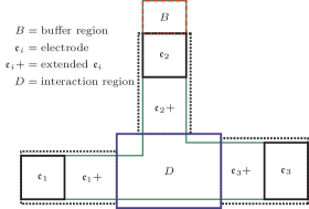
Figure 1: Conceptual system setup for a 3-electrode ($N_{\mathfrak{e}}=3$) example. The electrode regions are denoted by $\mathfrak{e}_{i}$ (black blocks) and the associated electrode screening regions by $\mathfrak{e}_{i}+$. The scattering/device region is indicated by $D$ (blue block). An additional buffer region $B$ (red block) denotes a region removed from the NEGF algorithm. All blocks as a whole represent the supercell used for a transiesta calculation.

The specifics governing the underlying methodology (siesta) for atomic-like basis-sets can be found elsewhere Soler et al. (2002); Brandbyge et al. (2002). Figure 1 illustrates the kind of generic multi-electrode NEGF setup we have in mind in the remainder of the paper. For setups where periodic boundary conditions with given lattice vectors $\mathbf{R}$, we apply Bloch $\mathbf{k}$-point sampling possible for both the DFT-NEGF self-consistent calculation and the subsequent transport calculation. To keep clarity, we explicitly add the $\mathbf{k}$ dependence to the equations while $\mathfrak{e}$ refers to an electrode index. Furthermore we write all equations generically with $N_{\mathfrak{e}}$ electrodes to clarify specifics related to any number of electrodes; $N_{\mathfrak{e}}\geq 1$. The following expressions are used throughout the paper

$$\mathbf{G}_{\mathbf{k}}(z) =\Big{[}z\mathbf{S}_{\mathbf{k}}-\mathbf{H}_{\mathbf{k}}-\sum_{\mathfrak{e}}\boldsymbol{\Sigma}_{\mathfrak{e},\mathbf{k}}(z)\Big{]}^{-1},\quad\text{ with $z\equiv\epsilon+i\eta$,}$$ (1)

$$\boldsymbol{\Gamma}_{\mathfrak{e},\mathbf{k}}(z) =i\big{[}\boldsymbol{\Sigma}_{\mathfrak{e},\mathbf{k}}(z)-\boldsymbol{\Sigma}^{\dagger}_{\mathfrak{e},\mathbf{k}}(z)\big{]},$$ (2)

$$\mathcal{A}_{\mathfrak{e},\mathbf{k}}(z) =\mathbf{G}_{\mathbf{k}}(z)\boldsymbol{\Gamma}_{\mathfrak{e},\mathbf{k}}(z)\mathbf{G}_{\mathbf{k}}^{\dagger}(z),$$ (3)

$$\boldsymbol{\rho} =\frac{1}{2\pi}\iint_{\mathrm{BZ}}\!\!\!\!\!\!\mathrm{d}\mathbf{k}\mathrm{d}\epsilon\,\sum_{\mathfrak{e}}\mathcal{A}_{\mathfrak{e},\mathbf{k}}(z)n_{F,\mathfrak{e}}(\epsilon)e^{-i\mathbf{k}\cdot\mathbf{R}},$$ (4)

where $\mathbf{G}_{\mathbf{k}}$/$\mathbf{G}_{\mathbf{k}}^{\dagger}$ is the retarded/advanced Green function at energy $\epsilon$ (with a small positive constant $\eta=0^{+}$), and $\mathbf{H}_{\mathbf{k}}=\mathbf{H}e^{i\mathbf{k}\cdot\mathbf{R}}$, $\mathbf{S}_{\mathbf{k}}=\mathbf{S}e^{i\mathbf{k}\cdot\mathbf{R}}$, the Hamiltonian and overlap matrix at $\mathbf{k}$ in the scattering region with $\mathbf{R}$ being a lattice vector in the periodic directions. The self-energy and spectral function of electrode $\mathfrak{e}$ are $\boldsymbol{\Sigma}_{\mathfrak{e}}$ and $\mathcal{A}_{\mathfrak{e}}$, respectively, with associated broadening matrix $\boldsymbol{\Gamma}_{\mathfrak{e}}$. Lastly, $\boldsymbol{\rho}$ is the non-equilibrium density matrix. BZ denotes here, and in the following, the Brillouin zone average (i.e., it includes a normalization corresponding to the appropriate Brillouin zone volume). Equation (4) is the density matrix for equilibrium and non-equilibrium (disregarding bound states). We require a Hermitian Hamiltonian and express the chemical potential as $\mu$, and the temperature as $k_{B}T$. A combined quantity is defined $\varsigma\equiv\{\mu,k_{B}T\}$. We will freely denote a Fermi distribution by $n_{F,\varsigma}$ as well as $n_{F,\mathfrak{e}}$ where the latter implicitly refers to $\varsigma$ belonging to the electrode $\mathfrak{e}$. transiesta is also implemented with spin-polarization and we will omit the factor of $2$ for non-polarized calculations, thus equations are for one spin-channel, unless otherwise stated. Lastly, we omit using the so-called “transport direction” which is ill-defined for nonparallel electrodes. As such our implementation of transiesta only deals with the semi-infinite directions of each electrode. This is apparent in $N_{\mathfrak{e}}>2$ calculations as performed in Refs. Palsgaard et al. (2015); Jacobsen et al. (2016).

Finally, we define another central quantity for the Green function technique, namely the energy density matrix $\boldsymbol{\mathcal{E}}$, as

$$\boldsymbol{\mathcal{E}}=\frac{1}{2\pi}\iint_{\mathrm{BZ}}\!\!\!\!\!\!\mathrm{d}\mathbf{k}\mathrm{d}\epsilon\,\epsilon\sum_{\mathfrak{e}}\mathcal{A}_{\mathfrak{e},\mathbf{k}}(z)n_{F,\mathfrak{e}}(\epsilon)e^{-i\mathbf{k}\cdot\mathbf{R}},$$ (5)

which enables force calculations under non-equilibrium situations Di Ventra and Pantelides (2000); Brandbyge et al. (2003).

II.1 Equilibrium (EGF)

In (global) equilibrium all Fermi distribution functions are equal, i.e., $n_{F,\mathfrak{e}}(\epsilon)=n_{F}(\epsilon)$, and Eq. (4) can be reduced to

$$\boldsymbol{\rho}_{\mathrm{eq}}=\frac{i}{2\pi}\iint_{\mathrm{BZ}}\!\!\!\!\!\!\mathrm{d}\mathbf{k}\mathrm{d}\epsilon\left[\mathbf{G}_{\mathbf{k}}(z)-\mathbf{G}^{\dagger}_{\mathbf{k}}(z)\right]n_{F}(\epsilon)e^{-i\mathbf{k}\cdot\mathbf{R}}.$$ (6)

To circumvent the meticulous and tedious integration in Eq. (6) along the energy axis, it is advantageous to use the residue theorem Brandbyge et al. (2002). The advantage is that the Green function, which varies quickly near the poles on the real axis, is analytic and much smoother in the complex plane, which in turn allows for numerically accurate quadrature methods. An example of the smoothing in the complex plane can be found in the supplementary material (SM). As the Green function has poles on the real axis (the eigenvalues of its inverse) and the Fermi function $n_{F}$ has poles at $z_{\nu}=ik_{B}T\pi(2\nu+1)$ with $\operatorname{Res}n_{F}(z_{\nu})=k_{B}T$ for $\nu\in\mathbb{N}$, we have according to the residue theorem that

$$\oint\mathrm{d}z\big{[}\mathbf{G}_{\mathbf{k}}(z)-\mathbf{G}_{\mathbf{k}}^{\dagger}(z)\big{]}n_{F}(z)=-2\pi ik_{B}T\sum_{z_{\nu}}\big{[}\mathbf{G}_{\mathbf{k}}(z_{\nu})-\mathbf{G}_{\mathbf{k}}^{\dagger}(z_{\nu})\big{]},$$ (7)

which follows if $z\in\mathbb{R}+i\eta$, $\eta\to 0^{+}$.

An example of two different, but mathematically equivalent, contours are shown in Fig. 2a. To calculate the real axis integral one divides the enclosed contour into the integral along the real axis and the remaining of the contour. We note that $n_{F}(z)\to 0$ for $\Re z\gg E_{F}$ which avoids the need for a fully enclosed contour as $\lim_{z\to\infty+i\eta}\int_{\mathcal{R}_{\mathrm{up}}}^{(\mathcal{S/L})_{\mathrm{up}}}\mathrm{d}zf(z)n_{F}(z)\to 0$. We stress that all enclosed contours in the lower/upper complex plane are mathematically equivalent, as long as the lower bound is below the lowest eigenvalue in the Brillouin zone. The residue theorem can be applied two times for $\mathbf{G}_{\mathbf{k}}(z)-\mathbf{G}_{\mathbf{k}}^{\dagger}(z)$: We use the positive part of the imaginary coordinate system with $\operatorname{Im}z>0$ for integrating $\mathbf{G}_{\mathbf{k}}(z)$, and the negative part of the imaginary coordinate system with $\operatorname{Im}z<0$ for integrating $\mathbf{G}_{\mathbf{k}}^{\dagger}(z)$. This is indicated in Fig. 2a/b with $\mathcal{R}^{+/-}$, respectively. Importantly, the imaginary part of the line contour $\mathcal{L}/\mathcal{S}$ should be chosen large enough so that the Green function indeed is smooth. A higher number of poles increases the distance to the real axis. Thus one should take care of the number of poles used in the calculation as the imaginary part is solely determined by the temperature. For 10 poles and a temperature of $25\,\mathrm{meV}$ the imaginary part becomes $\sim 1.57\,\mathrm{eV}$. We emphasize that to ensure a consistent interpretation, irrespective of the electronic temperature, it is better to derive the number of poles from a fixed energy scale on the imaginary axis rather than choosing it directly. Furthermore, it is required that the lower bound of the contour integration is well below the lowest eigenvalue of the system as the Green function fans out when increasing the complex energy. See the SM for an interactive illustration of these points.

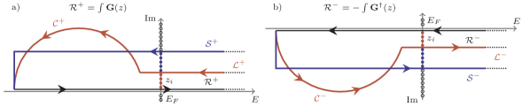
Figure 2: Two enclosing contours in the complex plane. The red contour is a circle contour while a square contour is shown by the blue line. Both are equivalent mathematically. The arrows indicate the direction of the contour integration. a) is the integration of the retarded Green function while b) is the advanced Green function. Note the sign change of the advanced Green function which results in an opposite direction integration.

II.2 Non-equilibrium (NEGF)

Non-equilibrium arises due to differences between the electrode electronic distributions via $\varsigma_{\mathfrak{e}}\neq\varsigma_{\mathfrak{e}^{\prime}}$. That is, either a chemical potential difference, an electronic temperature difference, or a combination of these. We define the bias window with a lower/upper bound as $\operatorname{min}(\mu_{\mathfrak{e}})$/$\operatorname{max}(\mu_{\mathfrak{e}})$ with appropriate tails of the Fermi functions. Starting from Eq. (4) and adding

$$0=(1-1)\sum_{\mathfrak{e}^{\prime}\neq\mathfrak{e}}\mathcal{A}_{\mathfrak{e}^{\prime},\mathbf{k}}(z)n_{F,\mathfrak{e}}(\epsilon)e^{-i\mathbf{k}\cdot\mathbf{R}},$$ (8)

(note that the products $\mathcal{A}_{\mathfrak{e}^{\prime},\mathbf{k}}(z)n_{F,\mathfrak{e}}(\epsilon)$ refer to different electrodes) we can write the density matrix as

$$\boldsymbol{\rho} =\boldsymbol{\rho}_{\mathrm{eq}}^{\mathfrak{e}}+\sum_{\mathfrak{e}^{\prime}\neq\mathfrak{e}}\boldsymbol{\Delta}_{\mathfrak{e}^{\prime}}^{\mathfrak{e}}\equiv\boldsymbol{\rho}_{\mathrm{neq}}^{\mathfrak{e}},$$ (9)

$$\boldsymbol{\rho}_{\mathrm{eq}}^{\mathfrak{e}} \equiv\frac{i}{2\pi}\iint_{\mathrm{BZ}}\!\!\!\!\!\!\mathrm{d}\mathbf{k}\mathrm{d}\epsilon\left[\mathbf{G}_{\mathbf{k}}(z)-\mathbf{G}^{\dagger}_{\mathbf{k}}(z)\right]n_{F,\mathfrak{e}}(\epsilon)e^{-i\mathbf{k}\cdot\mathbf{R}},$$ (10)

$$\boldsymbol{\Delta}_{\mathfrak{e}^{\prime}}^{\mathfrak{e}} \equiv\frac{1}{2\pi}\iint_{\mathrm{BZ}}\!\!\!\!\!\!\mathrm{d}\mathbf{k}\mathrm{d}\epsilon\,\mathcal{A}_{\mathfrak{e}^{\prime},\mathbf{k}}(z)e^{-i\mathbf{k}\cdot\mathbf{R}}\big{[}n_{F,\mathfrak{e}^{\prime}}(\epsilon)-n_{F,\mathfrak{e}}(\epsilon)\big{]},$$ (11)

where we call $\boldsymbol{\Delta}_{\mathfrak{e}^{\prime}}^{\mathfrak{e}}$ a non-equilibrium correction term for the equilibrium density of electrode $\mathfrak{e}$ due to electrode $\mathfrak{e}^{\prime}$. This reduces the real axis integral to be confined in the bias window with respect to the different Fermi distributions. Equation (9) deserves a few comments. It can be expressed equivalently for all electrodes $\mathfrak{e}$, and thus one finds $N_{\mathfrak{e}}$ different expressions for the same density $\boldsymbol{\rho}=\boldsymbol{\rho}_{\mathrm{neq}}^{\mathfrak{e}}=\boldsymbol{\rho}_{\mathrm{neq}}^{\mathfrak{e}^{\prime}}=\cdots$. If two or more electrodes have the same Fermi distribution, $\varsigma_{\mathfrak{e}}=\varsigma_{\mathfrak{e}^{\prime}}$, we find $\boldsymbol{\rho}_{\mathrm{eq}}^{\mathfrak{e}}=\boldsymbol{\rho}_{\mathrm{eq}}^{\mathfrak{e}^{\prime}}$ and $\boldsymbol{\Delta}_{\mathfrak{e}^{\prime}}^{\mathfrak{e}}=0$, thus we can reduce $N_{\mathfrak{e}}$ to $N_{\varsigma}$ different expressions. So for any $N_{\mathfrak{e}}>2$ electrodes with $2$ different Fermi distributions we only have $2$ equations with different terms (although the two equations are mathematically equivalent). We stress that the number of correction terms $\boldsymbol{\Delta}_{\mathfrak{e}^{\prime}}^{\mathfrak{e}}$ for each electrode depends on the number of equivalent Fermi distributions. Equivalently, Eq. (9) can be written more compactly as

$$\boldsymbol{\rho}=\boldsymbol{\rho}_{\mathrm{eq}}^{\varsigma}+\sum_{\mathclap{\mathfrak{e}|\varsigma_{\mathfrak{e}}\neq\varsigma}}\boldsymbol{\Delta}_{\mathfrak{e}}^{\varsigma}\equiv\boldsymbol{\rho}_{\mathrm{neq}}^{\varsigma},$$ (12)

where $\mathfrak{e}|\varsigma_{\mathfrak{e}}\neq\varsigma$ are electrodes with Fermi distributions different from $\varsigma$. Equation (9) is equivalent to Eq. (12) where the former have possible duplicates and the latter does not. These considerations also apply to the (non-equilibrium) energy density matrix, Eq. (5), in a similar manner.

Compared to the equilibrium case (Sec. II.1) we note that the non-equilibrium case is numerically more demanding in terms of matrix operations as the calculation of $\boldsymbol{\rho}$, in addition to the inversion for $\mathbf{G}_{\mathbf{k}}(z)$ needed in Eq. (6) and Eq. (10), also requires the evaluation of triple matrix products for $\mathcal{A}_{\mathfrak{e},\mathbf{k}}$, as seen in Eq. (11).

III Implementation details in transiesta

III.1 Complex contour optimization

The equilibrium contour in NEGF calculations can be chosen from a range of different shapes and methods to integrate. Here we describe the nontrivial task of selecting an optimum equilibrium contour. We have implemented several different methods, from Newton-Cotes to advanced quadrature methods, using Legendre polynomials or Tanh-Sinh quadrature Takahasi and Mori (1974). Both circle and square contours are possible. Furthermore the continued fraction method suggested by Ozaki Ozaki et al. (2010) is also implemented. Its strength is that it has only one convergence parameter, which is the number of poles, whereas the quadrature methods have (at least) three convergence parameters(number of poles ($z_{i}$), points on the line $\mathcal{L}^{+}$, and points on circle/square $\mathcal{C}^{+}/\mathcal{S}^{+}$).

A novel selection of quadrature points in $\mathcal{C}^{+}/\mathcal{S}^{+}$ can be realized by examining Fig. 2. It is evident that the two contours $\mathcal{C}^{+/-}$ for the retarded and advanced Green function add up to a connected circle. Hence we can consider them as one integration path and choose the quadrature to span the entire $\mathcal{C}^{+}+\mathcal{C}^{-}$ contour. In practice one only chooses the right half of the abscissa on the $\mathcal{C}^{+}+\mathcal{C}^{-}$ contour and effectively one uses a half quadrature on the $\mathcal{C}^{+}$ contour. We will denote this as the right-side scheme. This trick allows one to slightly reduce the number of equilibrium contour points without loss of accuracy.

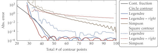
Figure 3: Test calculation on a metallic one-dimensional gold chain using Gaussian quadrature methods. Comparison of the square contour vs. the circle contour using the variants of integration methods: Regular Legendre, Legendre-right-side and Simpson quadrature. The Legendre-right-side seems better or at least on-par with the regular Legendre quadrature on the circle contour.

In order to illustrate the convergence properties of the equilibrium contour we have investigated a two-electrode gold (slab) system which is connected via a one-dimensional (1D) chain and calculated the free energy as a function of contour points. As the convergence path is non-deterministic and the “correct” value cannot be found we define the error against the free energy calculated with 300 energy points on the respective contour. As such the reference is itself. We stress that this study is difficult to extrapolate to arbitrary systems, yet it can be indicative of the convergence properties for the different quadrature methods and illustrates how critical the choice of method can be. The results are seen in Fig. 3. The circle and square quadratures have $16$ poles and the circle uses $10$ $\mathcal{L}^{+}$ points. Both the circle and square contours are presented using both the standard and the right-side scheme as well as the continued fraction method. Note that the numerical accuracy limits the error to $10^{-6}$.

We see that the circle contour benefits from the right-side scheme which performs the best in this setup. On the contrary, the square contour does not benefit from the right-side scheme. Furthermore, we see a slow convergence of the Simpson method (order 3 of Newton-Cotes method). Lastly, the continued fraction scheme Ozaki et al. (2010) converges fast and indeed is a powerful method due to its simplicity. We stress that changing the initial $\mathcal{L}^{+}$ and/or number of poles will change the convergence properties of the shown methods.

III.2 Weighing $\boldsymbol{\rho}$ and bound states

As shown in Sec. II.2 several different expressions exist for the non-equilibrium density matrix $\boldsymbol{\rho}_{\mathrm{neq}}$, depending on the choice of electrode for the equilibrium part in Eq. (9) and Eq. (12). Under non-equilibrium conditions these expressions numerically yield different densities, in particular if bound states are present. Per definition bound states do not couple to any of the electrodes via the spectral function, i.e., $\langle\psi_{\mathrm{bound}}|\mathcal{A}_{\mathfrak{e}}|\psi_{\mathrm{bound}}\rangle=0$. Their contributions to the non-equilibrium density $\boldsymbol{\rho}_{\mathrm{neq}}$ thus only derive from Eq. (10) – but never from Eq. (11) – as bound states are included in the electronic spectrum of $\mathbf{G}_{\mathbf{k}}(z)$. The filling level of bound states thus depends on the choice of equilibrium electrode in Eq. (10).

To avoid the arbitrariness of selecting one equilibrium electrode, and to reduce numerical errors, the physical quantity $\boldsymbol{\rho}_{\mathrm{neq}}$ is expressed as an appropriate average over each of the numerically unequal expressions

$$\boldsymbol{\rho}_{\mathrm{neq}}=\sum_{\mathfrak{e}}w_{\mathfrak{e}}\boldsymbol{\rho}_{\mathrm{neq}}^{\mathfrak{e}},$$ (13)

where $w_{\mathfrak{e}}$ is an appropriately chosen weight function satisfying $\sum_{\mathfrak{e}}w_{\mathfrak{e}}=1$. Several DFT-NEGF implementations apply such a weighing scheme, but with differences in the particular choice of weights $w_{\mathfrak{e}}$ Brandbyge et al. (2002); Li et al. (2007); Saha et al. (2009). We extend the argumentation of Ref. Brandbyge et al. (2002) for the weighing to a multi-terminal expression, and find the weights that minimize the variance of the final density to be

$$\boldsymbol{\theta}_{\mathfrak{e}}=\sum_{\mathfrak{e}^{\prime}\neq\mathfrak{e}}\operatorname{Var}[\boldsymbol{\Delta}^{\mathfrak{e}}_{\mathfrak{e}^{\prime}}],$$ (14)

$$w_{\mathfrak{e}}=\prod_{\mathfrak{e}^{\prime}\neq\mathfrak{e}}\boldsymbol{\theta}_{\mathfrak{e}^{\prime}}\Big{/}\Big{(}\sum_{\mathfrak{e}^{\prime}}\prod_{\mathfrak{e}^{\prime\prime}\neq\mathfrak{e}^{\prime}}\boldsymbol{\theta}_{\mathfrak{e}^{\prime\prime}}\Big{)},$$ (15)

where $\operatorname{Var}[\boldsymbol{\Delta}^{\mathfrak{e}^{\prime}}_{\mathfrak{e}}]\equiv(\boldsymbol{\Delta}^{\mathfrak{e}^{\prime}}_{\mathfrak{e}})^{2}$ is the expected variance of the correction term which is defined similarly to Ref. Brandbyge et al. (2002). The derivation of the expression for $w_{\varsigma}$ is in the SM. Additionally, 12 different weighing schemes have been checked to infer whether they might provide a better estimate of $\boldsymbol{\rho}_{\mathrm{neq}}$. However, we have found that the argumentation in Ref. Brandbyge et al. (2002) provides the best physical interpretation and also the best weighing. It is outside the scope of this paper to document their differences, yet they are available for end users.

If bound states are present in the system we weigh each equilibrium contribution equally. An example of the ambiguity of selecting the proper weight of bound states can be found in the SM.

III.3 Inversion algorithms and performance

siesta uses localized basis-orbitals (LCAO) which inherently introduce sparse Hamiltonian, density, and overlap matrices. The sparsity of the density matrix means that one only needs to compute the Green function for the appropriate non-zero elements. Further, in the NEGF formalism this computation relies on the inversion of the Hamiltonian and the overlap matrices (and self-energies). It is then beneficial to utilize specialized algorithms that can deal with this selected inversion.

Several inversion strategies have been explored Amestoy et al. (2000, 2001); Brandbyge et al. (2002); Petersen et al. (2008); Lin et al. (2009); Li et al. (2008); Lin et al. (2011a, b); Jacquelin et al. (2014, 2015); Hetmaniuk et al. (2013); Okuno and Ozaki (2013); Feldman et al. (2014); Thorgilsson et al. (2014) which all have their advantages and disadvantages. The MUMPS and SelInv methods are very efficient for calculating a small subset of the inverse matrix (EGF), while for dense parts of the matrix they are less effective (NEGF) Amestoy et al. (2000, 2001); Lin et al. (2011a, b); Jacquelin et al. (2014, 2015). transiesta originally implemented direct inversion using LAPACK Anderson et al. (1999); Brandbyge et al. (2002).

In the following we will present 3 different inversion algorithms Godfrin (1991); Amestoy et al. (2000, 2001); Brandbyge et al. (2002); Hod et al. (2006); Petersen et al. (2008); Reuter and Hill (2012), 1) direct (LAPACK), 2) sparse (MUMPS) and 3) block-tri-diagonal (BTD). The methods are all implemented in two variants, $\Gamma$-only ($\mathbf{k}=0$) and arbitrary $\mathbf{k}$-point, to limit memory usage where applicable. In the following we omit the explicit $\mathbf{k}$-dependence without loss of generality. For the non-equilibrium part of the contour a triple product of a Green function block column is required to calculate the spectral function in the non-zero elements of the density matrix. To calculate the spectral function, the needed block columns are those where $\boldsymbol{\Gamma}_{\mathfrak{e}}$ is non-zero, i. e.

$$\mathcal{A}_{\mathfrak{e}}(z)=\mathbf{G}(z)\boldsymbol{\Gamma}_{\mathfrak{e}}(z)\mathbf{G}^{\dagger}(z)={\begin{tabular}[]{|@{}ccc@{}|}\hline\cr\rule{5.69046pt}{5.69046pt}&\rule{5.69046pt}{5.69046pt}&\rule{5.69046pt}{5.69046pt}\\ \rule{5.69046pt}{5.69046pt}&\rule{5.69046pt}{5.69046pt}&\rule{5.69046pt}{5.69046pt}\\ \rule{5.69046pt}{5.69046pt}&\rule{5.69046pt}{5.69046pt}&\rule{5.69046pt}{5.69046pt}\\ \hline\cr\end{tabular}\,\begin{tabular}[]{|@{}ccc@{}|}\hline\cr\rule{5.69046pt}{5.69046pt}&&\\ &\color[rgb]{1,1,1} \rule{5.69046pt}{5.69046pt}&\\ &&\color[rgb]{1,1,1} \rule{5.69046pt}{5.69046pt}\\ \hline\cr\end{tabular}\,\begin{tabular}[]{|@{}ccc@{}|}\hline\cr\rule{5.69046pt}{5.69046pt}&\rule{5.69046pt}{5.69046pt}&\rule{5.69046pt}{5.69046pt}\\ \rule{5.69046pt}{5.69046pt}&\rule{5.69046pt}{5.69046pt}&\rule{5.69046pt}{5.69046pt}\\ \rule{5.69046pt}{5.69046pt}&\rule{5.69046pt}{5.69046pt}&\rule{5.69046pt}{5.69046pt}\\ \hline\cr\end{tabular}^{\dagger}=\begin{tabular}[]{|@{}ccc@{}|}\hline\cr\rule{5.69046pt}{5.69046pt}&&\\ \rule{5.69046pt}{5.69046pt}&\color[rgb]{1,1,1} \rule{5.69046pt}{5.69046pt}&\\ \rule{5.69046pt}{5.69046pt}&&\color[rgb]{1,1,1} \rule{5.69046pt}{5.69046pt}\\ \hline\cr\end{tabular}\,\begin{tabular}[]{|@{}ccc@{}|}\hline\cr\rule{5.69046pt}{5.69046pt}&&\\ &\color[rgb]{1,1,1} \rule{5.69046pt}{5.69046pt}&\\ &&\color[rgb]{1,1,1} \rule{5.69046pt}{5.69046pt}\\ \hline\cr\end{tabular}\,\begin{tabular}[]{|@{}ccc@{}|}\hline\cr\rule{5.69046pt}{5.69046pt}&&\\ \rule{5.69046pt}{5.69046pt}&\color[rgb]{1,1,1} \rule{5.69046pt}{5.69046pt}&\\ \rule{5.69046pt}{5.69046pt}&&\color[rgb]{1,1,1} \rule{5.69046pt}{5.69046pt}\\ \hline\cr\end{tabular}^{\dagger}}.$$ (16)

Equation (16) is implemented for the 3 inversion algorithms which substantially reduces memory requirements, and particularly so for the BTD method.

III.3.1 Block-tri-diagonal inversion

Our block-tri-diagonal matrix inversion algorithm has become the default method in transiesta. This algorithm was originally described in Ref. Godfrin (1991) while we follow the simpler outlined form in Refs. Hod et al. (2006); Reuter and Hill (2012). Often, this method is known as the recursive Green function method which corresponds to creating a quasi 1D, block tri-diagonal matrix.

Figure 4: Block-tri-diagonal inversion algorithm shown in terms of the Hamiltonian elements of a 2-electrode system. The inverse Greens function consists of block matrices in the diagonal and lower/upper diagonals denoted by $\mathbf{A}_{i}$ and $\mathbf{B}_{i}$/$\mathbf{C}_{i}$, respectively. The surface self-energies are calculated from the bulk electrode and the self-energies are propagated through the system, allowing one to calculate the exact Green function in any block of the infinite matrix.

The algorithm can be illustrated as shown in Fig. 4 and follow these equations

$$\mathbf{\mathbf{G}}^{-1} =\begin{pmatrix}\mathbf{A}_{1}&\mathbf{C}_{2}&0&\cdots&\\ \mathbf{B}_{1}&\mathbf{A}_{2}&\mathbf{C}_{3}&0&\cdots\\ 0&\mathbf{B}_{2}&\ddots&\ddots&0\\ \vdots&0&\ddots&\ddots&\mathbf{C}_{p}\\ &\vdots&0&\mathbf{B}_{p-1}&\mathbf{A}_{p}\\ \end{pmatrix}, \quad\begin{aligned} \widetilde{\mathbf{Y}}_{n}&=\left[\mathbf{A}_{n-1}-\mathbf{Y}_{n-1}\right]^{-1}\mathbf{C}_{n},&&\mathbf{Y}_{1}=0,\\ \mathbf{Y}_{n}&=\mathbf{B}_{n-1}\widetilde{\mathbf{Y}}_{n}.\\ \widetilde{\mathbf{X}}_{n}&=\left[\mathbf{A}_{n+1}-\mathbf{X}_{n+1}\right]^{-1}\mathbf{B}_{n},&&\mathbf{X}_{p}=0,\\ \mathbf{X}_{n}&=\mathbf{C}_{n+1}\widetilde{\mathbf{X}}_{n},\end{aligned}$$ (17)

$\mathbf{A}_{i}$, $\mathbf{B}_{i}$ and $\mathbf{C}_{i}$ correspond to the non-zero elements of $z\mathbf{S}-\mathbf{H}-\sum_{\mathfrak{e}}\boldsymbol{\Sigma}_{\mathfrak{e}}$, cf. Eq. (1). $\mathbf{Y}_{n}$/$\mathbf{X}_{n}$ can be thought of as the self-energies connecting to a previous sequence of $\mathbf{Y}_{m}$/$\mathbf{X}_{m}$ for $n>m$/$m>n$. These are sometimes denoted the “downfolded” self-energies and are indicated in Fig. 4. For instance $\mathbf{Y}_{2}$ corresponds to a self-energy of an infinite bulk part connecting to $\mathbf{A}_{1}$. Note that only for a Left/Right terminal system with strict ordering of orbitals will $\mathbf{A}_{1}=z\mathbf{S}_{1,1}-\mathbf{H}_{1,1}-\boldsymbol{\Sigma}_{\mathrm{Left}}$ and $\mathbf{A}_{p}=z\mathbf{S}_{p,p}-\mathbf{H}_{p,p}-\boldsymbol{\Sigma}_{\mathrm{Right}}$. Importantly the $\widetilde{\mathbf{Y}}_{i}$/$\widetilde{\mathbf{X}}_{i}$ matrices can be calculated using a linear solution instead of an inversion and subsequent matrix-multiplication. The strict ordering of the self-energies is not a requirement and $\boldsymbol{\Sigma}_{\mathfrak{e}}$ may be split among any sub-matrices $\mathbf{A}_{i}$, $\mathbf{B}_{i}$ or $\mathbf{C}_{i}$. Calculating any part of the Green function then follows the iterative solution of these equations

$$\left.\begin{aligned} \mathbf{G}_{n,n}&=\left[\mathbf{A}_{n}-\mathbf{X}_{n}-\mathbf{Y}_{n}\right]^{-1},\\ \mathbf{G}_{m-1,n}&=-\widetilde{\mathbf{Y}}_{m}\mathbf{G}_{m,n}\quad\text{ for }m\leq n,\\ \mathbf{G}_{m+1,n}&=-\widetilde{\mathbf{X}}_{m}\mathbf{G}_{m,n}\quad\text{ for }m\geq n,\end{aligned}\qquad\right\}\quad\mathbf{G}=\begin{aligned} \includegraphics{G_recursion}\end{aligned}$$ (18)

The algorithm for the above calculation is shown in Fig. 5.

For the non-equilibrium part the straightforward implementation of the column product in Eq. (16) involves calculating the full Green function column for columns of the scattering matrix and a subsequent triple matrix product for each block. However, it may be advantageous to utilize the propagation of the spectral function by using Eqs. (18) which inserted into Eq. (16) yields

$$\mathcal{A}_{\mathfrak{e}}=\begin{aligned} \includegraphics{A_recursion}\end{aligned}.$$ (19)

Recall that $\mathcal{A}_{\mathfrak{e},i,i}=\mathbf{G}_{i,i}\boldsymbol{\Gamma}_{\mathfrak{e}}\mathbf{G}^{\dagger}_{i,i}$. Importantly Eqs. (19) are recursive equations similar to Eqs. (18). The propagation of the spectral function is often faster than the straightforward method. The algorithm for the propagation method is shown in Fig. 5. To reduce computations we calculate $\widetilde{\mathbf{X}}_{i}$, $\widetilde{\mathbf{Y}}_{i}$ and the diagonal Green function elements where $\boldsymbol{\Gamma}_{\mathfrak{e}}$ lives for all $N_{\mathfrak{e}}$ and store these quantities in one BTD matrix. Subsequently we calculate the spectral function for each electrode separately in another BTD matrix (without re-calculating $\widetilde{\mathbf{X}}_{i}$, $\widetilde{\mathbf{Y}}_{i}$) to drastically reduce computations.

It is important to note that the required elements of the density matrix are only those of the block-tri-diagonal matrix ($\mathbf{G}$ and $\mathcal{A}_{\mathfrak{e}}$) corresponding to the elements shown in Eq. (17). For $\mathbf{G}$, Eq. (18), one only calculates $\mathbf{G}_{i,i}$, $\mathbf{G}_{i+1,i}$ and $\mathbf{G}_{i,i+1}$ and similarly for $\mathcal{A}_{\mathfrak{e}}$. For the latter we only use the upper-left and lower-right algorithms as presented in Eq. (19).

EGF

1:allocate $\mathbf{M}$ and $\mathbf{N}$ with $p$ blocks

2:for all $\varsigma\in N_{\varsigma}$ do

3:     initialize all $\mathbf{A}_{i}$, $\mathbf{B}_{i}$, $\mathbf{C}_{i}$ in $\mathbf{M}$

4:     for all $i\in\{1,\dots,p-1\}$ do

5:         $\mathbf{N}_{i+1,i}\leftarrow\widetilde{\mathbf{Y}}_{i+1}$

6:         $\mathbf{N}_{p-i,p-i+1}\leftarrow\widetilde{\mathbf{X}}_{p-i}$

7:     end for

8:     for all $i\in\{1,\dots,p\}$ do

9:         $\mathbf{N}_{i,i}\leftarrow\mathbf{G}_{i,i}$

10:     end for

11:     for all $i\in\{1,\dots,p-1\}$ do

12:         $\mathbf{N}_{i+1,i}\leftarrow\mathbf{G}_{i+1,i}$

13:         $\mathbf{N}_{p-i,p-i+1}\leftarrow\mathbf{G}_{p-i,p-i+1}$

14:     end for

15:     $\boldsymbol{\rho}_{\mathrm{eq}}^{\varsigma}\leftarrow\mathbf{N}$

16:end for

NEGF

1:allocate $\mathbf{M}$ with $p$ blocks

2:allocate $\mathbf{N}$ with $p$ blocks

3:initialize all $\mathbf{A}_{i}$, $\mathbf{B}_{i}$, $\mathbf{C}_{i}$ in $\mathbf{M}$

4:for all $i\in\{1,\dots,p\}$ do

5:     for all $\mathfrak{e}\in\{1,\dots,N_{\mathfrak{e}}\}$ do

6:         if $\mathrm{any}(\mathrm{column}(\mathfrak{e}))\in\mathbf{M}_{i,i}$ then

7:              $\mathrm{calc}(i)\leftarrow\textbf{True}$

8:         else

9:              $\mathrm{calc}(i)\leftarrow\textbf{False}$

10:         end if

11:     end for

12:end for

13:for all $i\in\{1,\dots,p-1\}$ do

14:     $\mathbf{N}_{i+1,i}\leftarrow\widetilde{\mathbf{Y}}_{i+1}$

15:     $\mathbf{N}_{p-i,p-i+1}\leftarrow\widetilde{\mathbf{X}}_{p-i}$

16:end for

17:for all $i\in\mathrm{calc}(:)=\textbf{True}$ do

18:     $\mathbf{N}_{i,i}\leftarrow\mathbf{G}_{i,i}$ $\triangleright$ Only columns needed

19:end for

20:for all $\mathfrak{e}\in\{1,\dots,N_{\mathfrak{e}}\}$ do

21:     $\mathbf{M}_{i,i}\leftarrow\mathbf{G}_{i,i}\boldsymbol{\Gamma}_{\mathfrak{e}}\mathbf{G}_{i,i}^{\dagger}$

22:     for all $\{m,n\}\in\{1,\dots,p\}$ do

23:         if $m+n<2i$ then

24:              $\mathbf{M}_{m,n}\leftarrow\widetilde{\mathbf{Y}}_{m+1}\cdots\widetilde{\mathbf{Y}}_{i}\mathbf{G}_{i,i}\boldsymbol{\Gamma}_{\mathfrak{e}}\mathbf{G}_{i,i}^{\dagger}\widetilde{\mathbf{Y}}_{i}^{\dagger}\cdots\widetilde{\mathbf{Y}}_{n+1}^{\dagger}$

25:         else

26:              $\mathbf{M}_{m,n}\leftarrow\widetilde{\mathbf{X}}_{m-1}\cdots\widetilde{\mathbf{X}}_{i}\mathbf{G}_{i,i}\boldsymbol{\Gamma}_{\mathfrak{e}}\mathbf{G}_{i,i}^{\dagger}\widetilde{\mathbf{X}}_{i}^{\dagger}\cdots\widetilde{\mathbf{X}}_{n-1}^{\dagger}$

27:         end if

28:         $\mathbf{M}_{m,n}\leftarrow\mathbf{M}_{m,n}(-1)^{m+n}$

29:     end for

30:     $\boldsymbol{\rho}_{\mathrm{neq}}^{\mathfrak{e}}\leftarrow\mathbf{M}$

31:end for

Figure 5: The algorithm used for inverting a generic BTD matrix as well as columns for calculating the spectral function in NEGF calculations. The EGF algorithm is a direct recursive algorithm Reuter and Hill (2012), while the NEGF algorithm is a modification to reduce the memory requirement for calculating the spectral function.

III.3.2 Orbital pivoting for minimizing bandwidth

The performance of the BTD algorithm is determined solely by the bandwidth of the Hamiltonian matrix, i. e. the size of the $\mathbf{A}_{n}$ blocks. The bandwidth is an expression of the quasi 1D size of the system and is defined as

$$B(\mathbf{M})=\max\big{(}|i-j|\big{|}\mathbf{M}_{ij}\neq 0\big{)}.$$ (20)

Internally, the sparsity pattern in siesta is determined via the atomic input sequence. However, this sparsity pattern will rarely have the minimum bandwidth, particularly so for $N_{\mathfrak{e}}\neq 2$. To minimize the matrix bandwidth, and increase performance, we have implemented 5 different pivoting methods, 1) connectivity graph based on the Hamiltonian sparse pattern, 2) peripheral connectivity graph based on a longest-path solution before a connectivity graph between end-points, 3) Cuthill-Mckee Cuthill and McKee (1969), 4) Gibbs-Poole-Stockmeyer Gibbs et al. (1976), and 5) generalized Gibbs-Poole-Stockmeyer Wang et al. (2009). The first 2 are developed by the authors and exhibit a good bandwidth reduction of the matrix for a majority of systems. The latter 3 methods are used in interaction graphs with few nodal points which may be the reason for their, sometimes, poor bandwidth reduction capability in atomic structure calculations. For cases of many nodal points per point, such as for 3D bulk structures, each of the methods yield different optimal orderings. Currently there exists no omnipotent method for bandwidth reduction and we encourage checking the different methods for each system. One may greatly increase pivoting performance by using the atomic graph, rather than the orbital graph. Indeed there is, obviously, little to no difference between the atomic and orbital graphs.

Pivoting becomes increasingly important when considering $N_{\mathfrak{e}}>2$ electrodes as the quasi 1D block-partitioning becomes less obvious. In Fig. 6 we illustrate the naive block partition for $N_{\mathfrak{e}}=\{2,3,4\}$ together with an improved partitioning. For $N_{\mathfrak{e}}=2$ the naive is a good partitioning. The naive $N_{\mathfrak{e}}=3$ problem will create a big block for $p=2$ which will decrease performance. However, by grouping two electrodes the quasi-1D problem can be much improved. Grouping should be chosen to minimise all block sizes, e.g. if the self-energy bandwidth, Eq. (20), of $B(\boldsymbol{\Sigma}_{2})>B(\boldsymbol{\Sigma}_{1})+B(\boldsymbol{\Sigma}_{3})$ then branches $\boldsymbol{\Sigma}_{1}$ and $\boldsymbol{\Sigma}_{2}$ should swap places in Fig. 6b. Similarly for $N_{\mathfrak{e}}=4$ two groups occur for both ends of the quasi 1D matrix. The grouping of electrodes can easily be generalised for any $N_{\mathfrak{e}}$ electrodes dependent on the branch sizes.

a) $N_{\mathfrak{e}}=2$	b) $N_{\mathfrak{e}}=3$	c) $N_{\mathfrak{e}}=4$

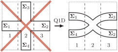
Figure 6: Quasi 1D partitioning in 3 parts (divided by dashed lines), for varying number of electrodes. The dotted lines denote the cell boundary and the fully drawn lines encompass the atoms/Hamiltonian elements. $\boldsymbol{\Sigma}_{i}$ are the self-energies that couple the device to the semi-infinite electrodes. The crossed illustrations are the naive partitioning of the quasi-1D system (the naive partitioning for $N_{\mathfrak{e}}=2$ is the best partitioning), whereas a better quasi-1D pivoting is also shown. Note that in any of the systems shown, the ordering of the self-energies can be swapped at will.

Pivoting complicates the triple product Eq. (16) due to partitioning of the scattering matrix with respect to the Green function. However, each block $\mathbf{A}_{n}$ can be sorted such that $\boldsymbol{\Gamma}_{\mathfrak{e}}$ becomes consecutive in memory for optimal performance. This will maximally split $\boldsymbol{\Gamma}_{\mathfrak{e}}$ into two blocks. We stress that splitting the broadening matrices, $\boldsymbol{\Gamma}_{\mathfrak{e}}$, up into two blocks, if possible, is more beneficial than retaining a single block because the bandwidth of the tri-diagonal matrix will be smaller.

III.3.3 Performance of inversion algorithms

A timing comparison of the three methods against transiesta 3.2 Brandbyge et al. (2002) is shown in Fig. 7. A pristine graphene system is used with square electrodes of 48 atoms, corresponding to $2\times 6$ (zigzag by armchair directions, respectively). Figure 7a show the timing for differing lengths of pristine graphene up to $\sim$6,000 orbitals using an EGF calculation. Figure 7b is the same calculation but with a high applied bias of $0.75\,\mathrm{V}$ (resulting in an equal amount of non-equilibrium and equilibrium contour points). MUMPS performs very well for EGF while NEGF is rather inefficient due to clustering of columns. Further studies of MUMPS have shown that it performs better for more than $\sim$5,000 orbitals as the sparsity increases. Lastly, the BTD method is performing extremely well reaching around 100 times better performance on systems at 5,000 orbitals. Doing even larger systems will only increase the speedup even more so. In all investigated systems we have found an impressive speedup for the BTD method.

III.3.4 Parallelization

Our inversion methods are parallelized across energy points, meaning that each MPI process handles one energy point on the contour, but needs to hold the complete (non distributed) matrices in memory. As the matrices dealt with in transiesta can become of GB size depending on the width of the electrodes, this parallelization scheme might hit the physical memory limit. To circumvent this we have updated the transiesta code to enable full hybrid parallelization with OpenMP 3.1 threading. Thus instead of using $N_{\mathrm{tot}}$ MPI processes and reaching the memory limit, one can use $N_{\mathrm{tot}}/N_{\mathrm{T}}$ processes and $N_{\mathrm{T}}$ threads per process. The threads pool their associated memory resources, pushing the practical limit by a factor of $N_{\mathrm{T}}$, and linear scaling is retained. Figure 7c shows the threading performance for transiesta on different hardware using a single node, hence MPI-communication can be considered negligible for hardware with multiple sockets. In our implementation an increase in the number of MPI processes would not affect the threading performance, however additional MPI processes would increase MPI communication time, thus favoring threading for large number of MPI processes.

The graphene test system consists of 11 BTD blocks with an average block size of $N_{B}=830$ using the $\mathbf{k}$-space version of the BTD method with a bias. We expect this system to represent a typical medium sized system of 9,130 orbitals. We find that there is extremely good scaling up to 4 threads. For higher number of threads the scaling is still good, but diverges. Threading is optimal for $N_{B}/N_{\mathrm{T}}\ggg 1$ which is one reason for the limiting speedup for large thread-counts in the shown data. By calculating the parallel fraction using Amdahl’s law we get roughly 95% across the investigated range of $N_{\mathrm{T}}$.

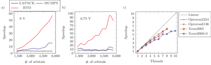
Figure 7: Performance characterization of transiesta using a pristine graphene cell (24 atoms wide). Speedup for (a) EGF and (b) NEGF calculations of pristine graphene compared against the direct LAPACK implementation. The BTD method exhibits more than 40 times the speed of the LAPACK implementation for the largest size. MUMPS gains speed after $5,000$ orbitals. (c) Threading performance using different hardware architectures running on a single node. Our test system has roughly 830 orbitals per BTD block and consists of 11 blocks in total. As the threading performance primarily stems from the threaded BLAS library one can see that the threading reaches a limit due to the rather small blocks.

III.4 Bloch theorem and self-energies

A performance-critical part of Green function implementations is an efficient calculation of the electrode self-energies. It is beneficial both computationally and in memory cost to calculate the self-energy using the smallest unit-cell which can be repeated to form the larger super-cell corresponding to the electrode-device contact region. In transiesta we utilize Bloch’s theorem and the corresponding $\mathbf{k}$-point sampling when transverse periodicity is present. The Bloch expansion may be used for both the electrode Hamiltonian and the self-energies, given that the electronic structure is calculated at equivalent $\mathbf{k}$ sampling, i.e., that an electrode which repeats out $X\times Y$ times in the larger device unit-cell, must be computed on $\mathbf{k}$ mesh which is $X\times Y$ more dense. Bloch expansion along one cell vector may be written in this short matrix form

$$\boldsymbol{\Sigma}_{k_{n}}^{n}=\frac{1}{n}\;\sum_{\mathclap{\begin{subarray}{c}j\\ k_{j}=k_{n}+2\pi\frac{j-1}{nR}\end{subarray}}}^{n}\qquad\begin{bmatrix}1&e^{-ik_{j}R}&\cdots&e^{-ink_{j}R}\\ e^{ik_{j}R}&1&\cdots&e^{-i(n-1)k_{j}R}\\ \vdots&\vdots&\ddots&\vdots\\ e^{ink_{j}R}&e^{i(n-1)k_{j}R}&\cdots&1\end{bmatrix}\otimes\boldsymbol{\Sigma}_{k_{j}}^{1},$$ (21)

where $\boldsymbol{\Sigma}^{n}$/$\boldsymbol{\Sigma}^{1}$ is the self-energy in the larger/smallest unit-cell and $n$ is the number of times the smallest unit-cell is repeated to coincide with the larger unit-cell. Here $R$ denotes the cell length of the small unit-cell. Lastly, $k_{n}$ is the $k$-point in the repeated super-cell. From Eq. (21) it can be inferred that one needs to calculate the self-energy $\boldsymbol{\Sigma}^{1}$ for $n$ $\mathbf{k}$ points instead of calculating $\boldsymbol{\Sigma}^{n}$ once. However, calculating the self-energy scales cubic and using a smaller matrix is far more beneficial.

III.5 Electrostatics in NEGF

The Hartree electrostatic potential plays an essential role for the NEGF calculations. In transiesta it is determined from the difference between the self-consistent electron density $\rho(\mathbf{r})$ and the neutral atom density $\rho^{\mathrm{atom}}(\mathbf{r})$ and solved using a Fourier transformation of the Poisson equation. transiesta implements a generic interface to correctly introduce the appropriate boundary conditions, fully controlled by the user.

For a reasonable description of the electrostatics in the NEGF setup one generally requires that the electrode regions in the device essentially behave as bulk. This requirement ensures a smooth electrostatic interface between the device and the semi-infinite, enforced bulk electrodes. For metallic electrodes this may easily be accomplished as the electronic screening length is short (typically a few atomic layers). Additionally we allow buffer atoms which are non-participating atoms in the scattering region calculation. They may be used to screen electrodes such that smaller scattering regions may be used. Such constructs are useful when non-periodic or dissimilar electrodes are used. Along side with buffer atoms several other methodologies for improving the electrode/device interface exists, such as forcing the density to be bulk, or calculating $\boldsymbol{\rho}$ in the electrode region.

In open boundary calculations, such as NEGF, one also needs to ensure that the Hartree potential fulfills the specific boundary conditions at the electrodes. We employ a formulation similar to the original implementation Brandbyge et al. (2002); Rocha et al. (2006). For $N_{\mathfrak{e}}=2$ and a shared semi-infinite direction a linear potential ramp can be used as a guess Brandbyge et al. (2002). For unaligned semi-infinite directions the boundary conditions become non-trivial. The simplest initial guess for the Hartree potential to fulfill the boundary conditions is a box guess

$$V_{H}(\mathbf{r})\leftarrow V_{H}(\mathbf{r})+\sum_{\mathfrak{e}}\begin{cases}\mu_{\mathfrak{e}}&\quad\text{, for $\mathbf{r}\in\mathbf{r}_{\mathfrak{e}}$}\\ 0&\quad\text{, for $\mathbf{r}\not\in\mathbf{r}_{\mathfrak{e}}$}\end{cases}$$ (22)

where $\mathbf{r}_{\mathfrak{e}}$ denotes the part in the real space grid where the electrode atoms reside. However, this introduces non-smooth potentials between the electrode and device region and it may only yield qualitative approximations to the actual Hartree potential. transiesta also allows custom Hartree potentials for improving convergence. It is recommended to provide a custom guess for $N_{\mathfrak{e}}>2$ as charge conservation and convergence can easily be improved. Note that the initial guess for the Hartree solution is linear in the difference between $\mu_{\mathfrak{e}}$, hence only one guess calculation of the Hartree potential is needed which makes this an in-expensive setup calculation. We have implemented a multigrid (MG) solver for the Poisson equation and applied it to a $N_{\mathfrak{e}}=6$ system with three different chemical potentials: [$-V/2$, $0$, $V/2$], see Fig. 8b. The grid overlaying the geometry corresponds to the guessed Poisson solution for the MG method at 4 iso-values, $V/2$ (blue), $-V/2$ (red), $V/10$ (orange) and $-V/10$ (yellow). The Poisson solution is linearly dependent on $V$ due to the linearity of the chemical potentials. The heavily colored atoms are electrodes, “behind” each electrode are 3 buffer atoms to retain a bulk-like electrode. It consists of three crossing linear chains with one carbon chain, one gold chain and one half-half carbon-gold chain. In Fig. 8a we plot the absolute charge difference from the expected charge after each SCF iteration for both the equilibrium case and for an applied bias of 1 V using two different initial guesses. All calculations settles after 8 iterations at nearly no charge difference. For the two non-equilibrium cases the custom MG method reduces the initial fluctuations compared to the box guess.

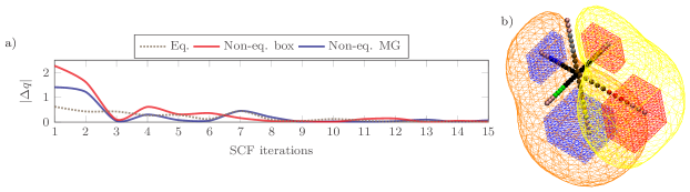
Figure 8: a) Charge conservation with respect to # of SCF iterations for a $N_{\mathfrak{e}}=6$ device (b). Both zero bias and two different initial guesses of the Hartree potential $V_{H}(\mathbf{r})$. The dashed curve is for equilibrium while the full lines are an electrode box guess and a full MG solution. Providing a better guess improves convergence. b) also shows the initial MG guess for 4 iso-values $\pm V/2$ and $\pm V/10$.

In addition to the electrostatics associated with complex boundary conditions we also extend siesta (and transiesta) by enabling electrostatic gates, as described in Ref. Papior et al. (2016). This allows to introduce additional non-interacting electrodes to act as gates. Several implementations of electrostatic Hartree gates use an explicit Hartree term $V_{H}(\mathbf{r})$ ATK (2014); Ozaki et al. (2010) while other implementations deal with the additional electrostatic terms arising from the charge distribution in the gate material Otani and Sugino (2006). We have implemented both a Hartree gate and a charge gate with few restrictions on the geometry of the gate. The geometries includes spherical, planes, rectangles and/or boxes are all allowed, further details can be found in Ref. Papior et al. (2016). The Hartree gate is similar to that in Refs. ATK (2014); Ozaki et al. (2010) while the charge gate is a phenomenological model resembling Refs. Otani and Sugino (2006); Brumme et al. (2014). Due to the simplicity of the Hartree gate we will instead focus here on explaining the charge gate method, with which one can simulate complex gate configurations in both NEGF and regular, 3D-periodic DFT calculations Papior et al. (2016).

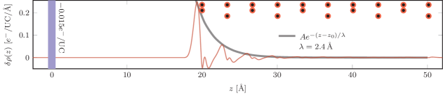
Figure 9: Electronic density decay length of a $10$-layer graphene stack. The red-black circles shows the placement of the carbon atoms (A-B stacking). The thin line show the difference in electronic density between the gated and non-gated system. The thick line shows a fitted decay profile of the gate-induced electronic density. A decay length of $2.4\,\text{\AA}$ is found at this particular gating level.

Figure 9 shows an example of a charge gate introduced in DFT periodic calculations containing $10$ graphene layers (AB stacking). The charge gate is placed $20\,\text{\AA}$ away from (and parallel with) the first graphene layer. A strong gate corresponding to $0.015e^{-}$ per graphene unit-cell is applied and the resulting charge re-distribution is dependent on the screening length of graphite. By fitting an exponential function to the charge response we calculate the decay length for the electronic screening length of the electric field. Note that this decay length is a function of the electric field and the doping level. The decay length of $\lambda=2.4\,\text{\AA}$ corresponds well to experimentally found values for similar gate levels Ohta et al. (2007). We have also tested this on fewer layers with consistent results.

III.6 Charge conservation

A recurring issue with NEGF calculations is excess charge compared to a charge neutral device region. Especially, for weakly screening systems and for non-equilibrium the SCF loop may converge slowly and with great difficulty due to larger deviations from charge neutrality in the beginning of the SCF loop Engelund et al. (2016). To remedy this we have implemented an option which introduces a shift in the potential inside the device region, $\!\mathrm{d}\epsilon$, which sometimes can push the SCF loop towards the self-consistent solution with a charge neutral device region or that the assumption of equilibrium in the electrodes

The potential shift is obtained from the requirement that the net charge of the device region, $q_{D}$, should be zero. We use the total device DOS, $D(\epsilon_{R})$, at an initial energy reference level, $\epsilon_{R}$, located in the bias window,

$$q_{D}=\delta q+D(\epsilon_{R})\,\!\mathrm{d}\epsilon=0\quad\Rightarrow\quad\!\mathrm{d}\epsilon=-\frac{\delta q}{D(\epsilon_{R})}\,.$$ (23)

We assume here that the DOS vary slowly on the scale of the bias and $k_{B}T$ such that the reference energy is not critical. To lowest perturbation order in the potential shift we get a change in the density matrix in terms of the spectral density matrix, $\Delta\boldsymbol{\rho}=\!\mathrm{d}\epsilon\,(d\boldsymbol{\rho}(\epsilon_{R})/d\epsilon)$, which when added to $\boldsymbol{\rho}$ in the SCF loop enforces a charge neutral device region. During the SCF-loop we then update the reference energy $\epsilon_{R}\leftarrow\epsilon_{R}+\!\mathrm{d}\epsilon$. When the SCF-loop has converged we can check the degree of charge neutrality $\delta q$ and potential shift, $\!\mathrm{d}\epsilon$. These should both be small such that the feature can be turned off in a restarted calculation and converge without being invoked. If this is not possible it may indicate that the device region has a too short screening region towards the electrodes or, for high bias, that the approximation of equilibrium density and potential in the electrodes is not adequate.

III.7 Thermoelectric effects under NEGF

To the authors knowledge, thermoelectric effects are currently only studied under equi-temperature distributions for NEGF calculations. However, in principle such effects require population statistics to be correctly described using self-consistent NEGF calculations. Our implementation naturally permits such generality as the chemical potential and electronic temperature can be set independently for each electrode.

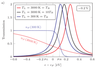
Figure 10: Example of a thermoelectric calculation for a simple 1D setup consisting of a central C atom weakly coupled to two perfect semiinfinite C-wires. a) Impact on the electronic transmission function $\mathcal{T}(\epsilon,V=-0.2\,\mathrm{eV})$ of the electrode temperatures $T_{L,R}$. The Fermi functions are also included for clarity of the difference in population. b) $IV$ characteristics computed from three distinct NEGF calculations (uniform temperature $T=300$, $3000\,\mathrm{K}$ vs temperature difference $T_{L}=3000\,\mathrm{K}$ and $T_{R}=300\,\mathrm{K}$) as detailed in the text.

As an example of how different electronic temperatures in the electrodes can impact the electronic structure in the device region we have performed calculations for a simple 1D setup consisting of a central C atom weakly coupled to two semi-infinite, 1D C-wires (lattice constant $a=1.30\,\text{\AA}$). The C-C distance between the central atom and the electrodes was set to $d=2.50\,\text{\AA}$. According to the band structure of the electrodes (not shown), the $2p_{x}$ and $2p_{y}$ orbitals on the equidistant lattice sites form a degenerate, half-filled band, which couples to the $2p_{x}$ and $2p_{y}$ orbitals of the central C-atom. This situation leads to the degenerate resonance structure in the transmission function as shown in Fig. 10a. Note that the position of this transmission resonance, i.e., the energetic position of the C-atom $2p_{x}$ and $2p_{y}$ orbitals, varies substantially for the three considered choices of the electrode temperatures. The thermoelectric calculations for the electron current shown in Fig. 10b correspond to the situation in which the electronic temperature of the left (right) electrode is fixed at $T_{L}=3000\,\mathrm{K}$ ($T_{R}=300\,\mathrm{K}$) in the Landauer formula, but where different temperature settings are used in the underlying self-consistent DFT-NEGF calculation as detailed in the figure legend.

These results exemplify that in situations with temperature differences between the electrodes, the fully self-consistent $IV$ characteristics (black curve in Fig. 10b) cannot be determined using a uniform temperature (red or blue curves in Fig. 10b). While the extreme temperature difference and narrow resonance at play in this example may seem far away from practical situations, we emphasize that it is generally desirable to be able to include this temperature effect at no additional computational cost. We further speculate that these methods could find relevance to describe situations with effective electronic temperatures substantially above the lattice temperature, e.g., as originating from optical driving Johannsen et al. (2013); Gierz et al. (2013).

IV Green function transport and techniques

As a post-processing tool for DFT-NEGF calculations of the self-consistent Hamiltonian, we have also developed the next-generation tbtrans (and its offshoot phtrans). tbtrans enables the calculation of electronic transport, electronic thermal energy transport, phonon transport (phtrans), and provide analysis tools such as the (spectral) density of states, the sub-partition eigenstate projected transmission (molecular or phonon eigenmode), interpolated $I$-$V$ curves, transmission eigenvalues and orbital/bond-currents Todorov (2002). Thus it is possible obtain thermoelectric quantities such as the Seebeck and Peltier coefficients as well as calculation of thermoelectric figure-of-merit including lattice heat-transport in the harmonic approximation. All features are enabled for general multi-electrode ($N_{\mathfrak{e}}\geq 1$) setups. The features discussed below – transmission functions, (spectral) density of states, sub-partition eigenstate projected transmissions, transmission eigenvalues, and bond-currents – encompass both the electronic and phononic versions, but for brevity we refer only to the electronic part in the following.

Besides input from DFT calculations tbtrans is also able to handle general user-created tight-binding models or by using Hamiltonians from other sources (Wannier basis, etc.). Thus tbtrans is now a stand-alone application capable of being used for large-scale, ballistic transport calculations. For example, simulations of square graphene flakes exceeding $10^{6}$ atoms may easily be done on typical office computers (one orbital/atom). An interface on top of tbtrans for creating corrections to DFT – such as scissor, LDA+U, magnetic fields, etc. – has also been created such that the capabilities of tbtrans are not restricted by the developers, but, in principle, by the user. This interface also allows the extraction of Hamiltonians from other programs to the tbtrans format. Other efficient methods involve similar constructs Mason et al. (2011); Ferrer et al. (2014).

IV.1 Transmission function for $N_{\mathfrak{e}}$ electrodes

The transmission functions can be calculated using the scattering matrix formalism and obtained from the Green function using the generalized Fisher-Lee relation Fisher and Lee (1981); Sanvito et al. (1999); Yeyati and Büttiker (2000) (or the Lippmann-Schwinger equation Lippmann and Schwinger (1950); Cook et al. (2011)). The elements of the scattering matrix, at a given $\mathbf{k}$, can be written as

$$s_{\mathfrak{e}\mathfrak{e}^{\prime},\mathbf{k}}=-\delta_{\mathfrak{e}\mathfrak{e}^{\prime}}\mathbf{I}+i\boldsymbol{\Gamma}_{\mathfrak{e},\mathbf{k}}^{1/2}\mathbf{G}_{\mathbf{k}}^{\phantom{/}}\boldsymbol{\Gamma}_{\mathfrak{e}^{\prime},\mathbf{k}}^{1/2},$$ (24)

where $\mathfrak{e}$ and $\mathfrak{e}^{\prime}$ refer to two electrodes and $\delta_{\mathfrak{e}\mathfrak{e}^{\prime}}$ is the Kronecker delta. We implicitly assume energy dependence on all quantities. The transmission (probability) from electrode $\mathfrak{e}$ to $\mathfrak{e}^{\prime}$ is

$$\mathcal{T}_{\mathfrak{e}\mathfrak{e}^{\prime},\mathbf{k}}=\operatorname{Tr}\big{[}s^{\dagger}_{\mathfrak{e}\mathfrak{e}^{\prime},\mathbf{k}}s^{\phantom{\dagger}}_{\mathfrak{e}\mathfrak{e}^{\prime},\mathbf{k}}\big{]}=\left\{\begin{aligned} &\operatorname{Tr}\big{[}\mathbf{G}_{\mathbf{k}}^{\phantom{\dagger}}\boldsymbol{\Gamma}^{\phantom{\dagger}}_{\mathfrak{e},\mathbf{k}}\mathbf{G}^{\dagger}_{\mathbf{k}}\boldsymbol{\Gamma}^{\phantom{\dagger}}_{\mathfrak{e}^{\prime},\mathbf{k}}\big{]},&\text{for $\mathfrak{e}\neq\mathfrak{e}^{\prime}$}\\ &\mathcal{R}_{\mathfrak{e},\mathbf{k}},&\text{for $\mathfrak{e}=\mathfrak{e}^{\prime}$}\end{aligned}\right.$$ (25)

where reflection (probability) is defined as $\mathcal{R}_{\mathfrak{e},\mathbf{k}}\equiv\mathcal{T}_{\mathfrak{e}\mathfrak{e},\mathbf{k}}$. It is instructive to write the aggregate transmission $\mathcal{T}_{\mathfrak{e},\mathbf{k}}$ out of an electrode $\mathfrak{e}$ (see Ref. Lake et al. (1997)) and the reflection $\mathcal{R}_{\mathfrak{e},\mathbf{k}}$ as

$$\mathcal{T}_{\mathfrak{e},\mathbf{k}} \equiv\sum_{\mathfrak{e}^{\prime}\neq\mathfrak{e}}\mathcal{T}_{\mathfrak{e}\mathfrak{e}^{\prime},\mathbf{k}}=i\operatorname{Tr}\big{[}(\mathbf{G}_{\mathbf{k}}^{\phantom{\dagger}}-\mathbf{G}_{\mathbf{k}}^{\dagger})\boldsymbol{\Gamma}_{\mathfrak{e},\mathbf{k}}^{\phantom{\dagger}}\big{]}-\operatorname{Tr}[\mathbf{G}_{\mathbf{k}}^{\phantom{\dagger}}\boldsymbol{\Gamma}_{\mathfrak{e},\mathbf{k}}^{\phantom{\dagger}}\mathbf{G}_{\mathbf{k}}^{\dagger}\boldsymbol{\Gamma}_{\mathfrak{e},\mathbf{k}}^{\phantom{\dagger}}],$$ (26)

$$\mathcal{R}_{\mathfrak{e},\mathbf{k}} =M_{\mathfrak{e},\mathbf{k}}-\mathcal{T}_{\mathfrak{e},\mathbf{k}}.$$ (27)

The reflection is here conveniently written as a difference between the bulk electrode transmission $M_{\mathfrak{e}}$ (i.e., number of open channels/modes in electrode $\mathfrak{e}$ at the given energy) and the aggregate transmission $\mathcal{T}_{\mathfrak{e}}$ (scattered part into the other electrodes). From Eqs. (25), (26) and (27) one may easily prove the transmission equivalence $\mathcal{T}_{\mathfrak{e}\mathfrak{e}^{\prime},\mathbf{k}}\equiv\mathcal{T}_{\mathfrak{e}^{\prime}\mathfrak{e},-\mathbf{k}}$ as well as $\mathcal{T}_{\mathfrak{e}\mathfrak{e}^{\prime},\mathbf{k}}=\mathcal{T}_{\mathfrak{e}\mathfrak{e}^{\prime},-\mathbf{k}}$ based on time-reversal symmetry. Equation (26) displays an important, and often overlooked detail. In transport calculations with $N_{\mathfrak{e}}=2$, one can calculate the transmission using only a sub-diagonal part of the Green function and only one scattering matrix. We stress that the quantities calculated may have numerical deficiencies as $\operatorname{Tr}[(\mathbf{G}-\mathbf{G}^{\dagger})\boldsymbol{\Gamma}_{\mathfrak{e}}]$ and $\operatorname{Tr}[\mathbf{G}\boldsymbol{\Gamma}_{\mathfrak{e}}\mathbf{G}^{\dagger}\boldsymbol{\Gamma}_{\mathfrak{e}}]$ may both be numerically large which leads to inaccuracies when the transmission is orders of magnitudes smaller than the reflection.

Further, the transmission may be split into transmission eigenvalues,

$$\mathcal{T}_{\mathfrak{e}\mathfrak{e}^{\prime},\mathbf{k}}=\sum_{i}\mathcal{T}_{i,\mathfrak{e}\mathfrak{e}^{\prime},\mathbf{k}}\,,$$ (28)

where $\mathcal{T}_{i,\mathfrak{e}\mathfrak{e}^{\prime},\mathbf{k}}$ are the eigenvalues of the column matrix $\mathbf{G}_{\mathbf{k}}\boldsymbol{\Gamma}_{\mathfrak{e},\mathbf{k}}\mathbf{G}_{\mathbf{k}}^{\dagger}\boldsymbol{\Gamma}_{\mathfrak{e}^{\prime},\mathbf{k}}$ ($\mathfrak{e}\neq\mathfrak{e}^{\prime}$) Paulsson and Brandbyge (2007). Due to the matrix product being a column matrix ($\boldsymbol{\Gamma}_{\mathfrak{e}}$ have a limited extend due to the LCAO basis) the eigenvalue calculation can be reduced substantially by realizing the following equation,

$$\det\big{(}\mathbf{G}_{\mathbf{k}}^{\phantom{\dagger}}\boldsymbol{\Gamma}_{\mathfrak{e},\mathbf{k}}^{\phantom{\dagger}}\mathbf{G}_{\mathbf{k}}^{\dagger}\boldsymbol{\Gamma}_{\mathfrak{e}^{\prime},\mathbf{k}}^{\phantom{\dagger}}-\lambda\mathbf{I}\big{)}=\det\Big{(}\begin{tabular}[]{|@{}ccc@{}|}\hline\cr\color[rgb]{1,1,1}\rule{5.69046pt}{5.69046pt}&&\rule{5.69046pt}{5.69046pt}\\ &\color[rgb]{1,1,1}\rule{5.69046pt}{5.69046pt}&\rule{5.69046pt}{5.69046pt}\\ &&\rule{5.69046pt}{5.69046pt}\\ \hline\cr\end{tabular}-\lambda\mathbf{I}\Big{)}=\det\left(\begin{bmatrix}\mathbf{0}&\mathbf{0}&\mathbf{A}\\ \mathbf{0}&\mathbf{0}&\mathbf{B}\\ \mathbf{0}&\mathbf{0}&\mathbf{C}\end{bmatrix}-\lambda\mathbf{I}\right)\to\det(\mathbf{C}-\lambda\mathbf{I}).$$ (29)

The transmission eigenvalues are for instance important when calculating Fano factors describing shot noise Schneider et al. (2012).

Once the transmission function is calculated we can calculate the electrical current $I_{\mathfrak{e}\mathfrak{e}^{\prime}}$ and thermal energy transfer $Q_{\mathfrak{e}\mathfrak{e}^{\prime}}$ as

$$I_{\mathfrak{e}\mathfrak{e}^{\prime}} =\frac{\mathrm{G}_{0}}{2|e|}\iint_{\mathrm{BZ}}\!\!\!\!\!\!\mathrm{d}\mathbf{k}\mathrm{d}\epsilon\,\mathcal{T}_{\mathfrak{e}\mathfrak{e}^{\prime},\mathbf{k}}(\epsilon)\big{[}n_{F,\mathfrak{e}^{\prime}}(\epsilon)-n_{F,\mathfrak{e}}(\epsilon)\big{]},$$ (30)

$$Q_{\mathfrak{e}\mathfrak{e}^{\prime}} =\frac{1}{h}\iint_{\mathrm{BZ}}\!\!\!\!\!\!\mathrm{d}\mathbf{k}\mathrm{d}\epsilon\,\mathcal{T}_{\mathfrak{e}\mathfrak{e}^{\prime},\mathbf{k}}(\epsilon)(\epsilon-\mu_{\mathfrak{e}})\big{[}n_{F,\mathfrak{e}^{\prime}}(\epsilon)-n_{F,\mathfrak{e}}(\epsilon)\big{]},$$ (31)

where $\mathrm{G}_{0}=2e^{2}/h$ is the conductance quantum (spin-degenerate case). When time-reversal symmetry applies one has the relations $I_{\mathfrak{e}\mathfrak{e}^{\prime}}=-I_{\mathfrak{e}^{\prime}\mathfrak{e}}$ and $Q_{\mathfrak{e}\mathfrak{e}^{\prime}}+Q_{\mathfrak{e}^{\prime}\mathfrak{e}}=(\mu_{\mathfrak{e}}^{\prime}-\mu_{\mathfrak{e}})/|e|I_{\mathfrak{e}\mathfrak{e}^{\prime}}\equiv W$. The latter expresses that the net work done, $W$, equals the net heat supplied.

We note that one may use efficient interpolation schemes for the BZ averages to reduce the required number of $\mathbf{k}$-points, which is typically much larger than the $\mathbf{k}$-sampling necessary for the corresponding density matrix calculation Falkenberg and Brandbyge (2015).

IV.2 Inversion algorithm — again

The Green function algorithm in tbtrans is similar to the one in transiesta (but not the same). In Figs. 1 and 11 we exemplify the method. In Fig. 11a we show a regular two-terminal device with $8$ partitions. In the BTD method one can down-fold the self-energy from the left $\infty$ block up till e.g. the block $6$, using Eq. (17), or as explained in Refs. Godfrin (1991); Petersen et al. (2008). Then the current is calculated using the standard Eq. (30) based on the transmission evaluated from the down-folded quantities calculating the Green function Eq. (18) and self-energies in the sub-space of block $6$. However, one could equally have chosen block $3$, or the combined blocks $3$ and $4$. The advantage of this abstraction is threefold: 1) the Green function is obtained in the chosen blocks of interest only, 2) choosing fewer blocks reduces the computational complexity which greatly speeds up the calculation, and 3) choosing small blocks reduces the required memory which enables extreme scale calculations. From 1) it follows that quantities such as local density of states can be calculated at arbitrary positions in the calculation cell by selecting specific blocks. However, we note that for non-orthogonal basis sets an increased block including the overlap region is required in order to obtain LDOS, Mulliken charges, etc. On the other hand, if one is only interested in the transmission/current one can resort to choosing the smallest block to achieve the highest throughput Petersen et al. (2008).

Similarly, down-folding of the self-energies can also be achieved in an $N_{\mathfrak{e}}$-terminal device. As an example, a 6-terminal system (e.g., the setup in Fig. 11b) can be split into several blocks with their own downfolding of self-energies. One chooses a region $D$ (see Fig. 1) and the extended electrode regions may be used to down-fold the self-energy. However, one may not choose $D$ such that either of the electrodes are directly coupled, since this choice would entangle the self-energies and their origin would be lost.

After selecting the region $D$, tbtrans creates $N_{\mathfrak{e}}+1$ different BTD matrices for optimal performance. These are $N_{\mathfrak{e}}$ BTD matrices for each electrode including the down-folding region ($\{\mathfrak{e}_{i},\mathfrak{e}_{i}+\}$ in Fig. 1), and one additional BTD matrix for region $D$. Each BTD matrix uses its own pivoting scheme to reduce the bandwidth and increase performance. Due to the pivoting, the Hamiltonian structure cannot be generically outlined in matrix format. Yet it can be formulated equivalently as in Ref. Ferrer et al. (2014) with the possibility of letting the user define the “extended scattering region”. tbtrans allows the user to do this via atomic indices, and hence no knowledge of the algorithms underlying the pivoting and other details are needed.

Figure 11: The BTD algorithm in tbtrans. a) Partitioning of a standard two-terminal setup for the recursive Green function method (BTD). b) Connectivity graph for the $N_{\mathfrak{e}}=6$ terminal device used in Fig. 8 where each dot represents an atom (non-black colored atoms correspond to an electrode) and every line represents one or multiple connections between the two atoms. Instead of calculating the Green function in the whole device space one can shrink the problem to a smaller region as long as the electrode branches do not couple directly to each other. An example region is shown with a dashed circle.

Lastly, we note that tbtrans is also implemented using OpenMP 3.1 threading and scales like shown in Fig. 7c for large systems.

IV.3 $I-V$ curves using Hamiltonian interpolation

Although the present work represents a significant leap in performance of transiesta and tbtrans, self-consistent NEGF calculations are still heavy, especially when current-voltage ($I-V$) characteristics with many bias points are required. To ease, and quite accurately, calculate $I-V$ curves we have implemented an interpolation scheme based on $N_{V}$ separate NEGF calculations at different bias conditions. If $N_{V}=2$ we do a linear interpolation/extrapolation of the Hamiltonian, and if $N_{V}>2$ a spline interpolation is also possible. Note that a spline extrapolation is equivalent, unsurprisingly, to linear extrapolation.

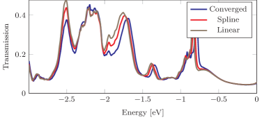
Figure 12: Interpolation of the transmission function for a Cu-tip–$\mathrm{C}_{60}$/Cu(111) junction using either spline or linear interpolation of the Hamiltonian at $V=-1.5\,\mathrm{V}$ using the converged Hamiltonians for $-2\,\mathrm{V}$, $-1\,\mathrm{V}$, $0\,\mathrm{V}$, $1\,\mathrm{V}$ and $2\,\mathrm{V}$. The spline interpolation (red curve) agrees significantly better with the self-consistent solution (blue curve) than the linear interpolation (brown curve).

As a test example we consider a molecular contact system consisting of a periodic array of $\mathrm{C}_{60}$ molecules buried in the first surface layer of a Cu(111) surface contacted by a tip. This example is taken from Ref. Schneider et al. (2015). In Fig. 12 we compare the $\mathbf{k}$-averaged transmission functions based on the self-consistent (converged) Hamiltonian at a bias of $-1.5\,\mathrm{V}$ and the corresponding one interpolated from self-consistent Hamiltonians at $-2\,\mathrm{V}$, $-1\,\mathrm{V}$, $0\,\mathrm{V}$, $1\,\mathrm{V}$ and $2\,\mathrm{V}$ (linear interpolation from the two closest bias points and spline using all points). In this example the bias point $-1.5\,\mathrm{V}$ was “worst case scenario” where the exact and interpolated results deviated the most out of 47 interpolations and extrapolations in the range $-2.4\,\mathrm{V}$ to $2.4\,\mathrm{V}$ (in equal steps of $0.1\,\mathrm{V}$). Although both interpolation schemes perform very well, the spline interpolation clearly outperforms the linear interpolation, retaining a better agreement with the self-consistent calculation. This also works for $N_{\mathfrak{e}}\neq 2$ if the chemical potentials are linearly dependent.

IV.4 tbtrans as transport back-end and feature generalization

Even though tbtrans is developed with transiesta in mind, its use is far from restricted to this. tbtrans implements flexible NetCDF-4 support, and the Hamiltonian can thus alternatively be supplied through a NetCDF-4 file. This makes tbtrans accessible as a generic transport code without a need for lower-level Fortran coding and/or knowledge of the siesta binary file format. To accommodate such so-called “tight-binding” calculations, we have developed a LGPL licensed Python package sisl Papior (2016) which facilitates an easy interface to create large-scale (non-)orthogonal tight-binding models for arbitrary geometries. This package is a generic package with further analysis tools for siesta such as file operations and grid operations (interaction with fdf-files, vasp files, and density grids, potential grids, etc.). sisl allows any number of atoms, different orbitals per atom, (non-)orthogonal basis sets, mixed species in a 3D super-cell approach. Furthermore, as sisl is based on Python it allows abstraction such that unnecessary details of the complex data structures are hidden from the users. Currently it is interfaced to read parameters from siesta, gulp and Wannier90 Gale and Rohl (2003); Mostofi et al. (2014).

import sisl
bond = 1.42
graphene = sisl.geom.graphene(bond)
# Create a 100x100x2 = 20000 atom graphene flake
flake = graphene.repeat(100, axis=0).tile(100, 1)
H = sisl.Hamiltonian(flake)
#       U          t1
dR = [0.1 * bond, 1.1 * bond]
for ia in flake:
    idx_a = flake.close(ia, dR=dR)
    # Define Hamiltonian elements
    H[ia,idx_a[0]] =  0.   # on-site
    H[ia,idx_a[1]] = -2.7  # nearest neighbor
H.write(’FLAKE.nc’)
    

import sisl
bond = 1.42
graphene = sisl.geom.graphene(bond)
flake = graphene.repeat(100, axis=0).tile(100, 1)
# Remove atoms in a circular region to create a hole
hole = flake.remove(flake.close(flake.center(), dR=10*bond))
H = sisl.Hamiltonian(hole)
dR = [0.1 * bond, 1.1 * bond]
for ia in hole:
    idx_a = hole.close(ia, dR=dR)
    # Define Hamiltonian elements
    H[ia,idx_a[0]] =  0.   # on-site
    H[ia,idx_a[1]] = -2.7  # nearest neighbor
H.write(’HOLE.nc’)
    

Figure 13: sisl code. Left: Creation of a periodic graphene flake with 20,000 atoms with nearest neighbor interactions ($\epsilon_{0}=0$ and $\epsilon_{1}=-2.7$). Right: Creation of a periodic graphene flake with a hole having a diameter of $20$ bond lengths.

In Fig. 13 we list two sisl-code examples. The left example creates a simple $20,000$ atom graphene flake with nearest neighbor interaction. The right example creates the same graphene structure but with a hole with a diameter of $20$ times the bond length at the center of the flake. In the SM we have added several example scripts for graphene with various tight-binding parameter sets Hancock et al. (2010) as well as an example of how to create a tight-binding transport calculation.

IV.4.1 Feature generalization – $\delta\mathbf{H}$

Green function codes are often limited by the implemented features. Yet a large scope of features can be described using a correction of the Hamiltonian elements due to local smearing, scissor operators, magnetic fields, the SAINT method García-Suárez and Lambert (2011), etc. All in all they can be summarized in this one equation

$$\mathbf{H}_{\mathbf{k}}\leftarrow\mathbf{H}_{\mathbf{k}}+\delta\mathbf{H}_{\mathbf{k}}(\epsilon),$$ (32)

where $\delta\mathbf{H}_{\mathbf{k}}(\epsilon)$ encompass any correction for the Hamiltonian, whatever that may be. $\delta\mathbf{H}_{\mathbf{k}}(\epsilon)$ may be of a real quantity, or a complex quantity, depending on its physical origin.

Instead of letting the developers decide which features should be implemented we enable users to create their own features by altering the Hamiltonian elements, however they wish, simply by creating the $\delta\mathbf{H}_{\mathbf{k}}(\epsilon)$ correction. sisl Papior (2016) efficiently creates the $\delta\mathbf{H}_{\mathbf{k}}(\epsilon)$ matrix without any prior knowledge of Fortran or the data format for tbtrans. We note that sisl is capable of reading the DFT-NEGF self-consistent Hamiltonian and edit it directly in Python.

The $\delta\mathbf{H}_{\mathbf{k}}(\epsilon)$ comes in four variants to control different parts of the calculation.

1. $\delta\mathbf{H}$ with no energy nor $\mathbf{k}$-point dependencies,

2. $\delta\mathbf{H}_{\mathbf{k}}$ with only $\mathbf{k}$-point dependency,

3. $\delta\mathbf{H}(\epsilon)$ with only energy dependency,

4. $\delta\mathbf{H}_{\mathbf{k}}(\epsilon)$ with both $\mathbf{k}$-point and energy dependencies.

This feature enables a broader population of users to contribute with functionality to a public code, and we encourage contributions to the siesta mailing list as well as the sisl GitHub repository which may be used as a base for further development of features for the transport code tbtrans.

IV.5 Molecular state projection transmission

There are several approaches to analyze transport properties besides considering the local density of states. One may decompose the transmission into eigenchannels and plot the corresponding scattering states Paulsson and Brandbyge (2007) or the bond-currents Solomon et al. (2010). However, this does not necessarily give a clear answer to the basic question as to which of the eigenstates in the central region takes part in transport, e.g., which molecular levels transmit the electrons in a molecular contact between metals. tbtrans allow a very flexible analysis of the transport through such eigenstates. In the following we use molecular eigenstates as the terminology and have a central molecule as “bottle-neck” in mind, however, the method is not limited to this type of setup.

We can define a sub-space of the full device region consisting of the same or fewer basis components $\{\!M\}$ (henceforth referred to as “molecule”). The Hamiltonian for this region have previously been denoted Molecular Projected Self-consistent Hamiltonian (MPSH) Stokbro et al. (2003) with corresponding eigenstates,

$$\mathbf{H}_{\{\!M\}}|M^{\prime}_{i}\rangle=\varepsilon_{i}^{\{\!M\}}\mathbf{S}_{\{\!M\}}|M^{\prime}_{i}\rangle,$$ (33)

where $|M^{\prime}_{i}\rangle$ are the generalized eigenvectors defined in the basis functions of the non-orthogonal basis. In order to create orthogonal eigenvectors ($|M_{i}\rangle$) we rotate the basis set to form orthonormal projection vectors using the Löwdin transformation Löwdin (1950).

Inserting the complete $\{\!M\}$ (orthogonalized) basis in the expression for the transmission (assuming $\mathbf{k}$ and $\epsilon$ dependencies implicit, and $\{\mathfrak{e},\mathfrak{e}^{\prime}\}=\{L,R\}$) we get

$$\mathcal{T}_{LR} =\operatorname{Tr}[\mathbf{G}\boldsymbol{\Gamma}_{L}\mathbf{G}^{\dagger}\boldsymbol{\Gamma}_{R}]$$ (34)

$$=\operatorname{Tr}\Big{[}\mathbf{G}\sum_{j}|M_{j}\rangle\langle M_{j}|\boldsymbol{\Gamma}_{L}\sum_{j^{\prime}}|M_{j^{\prime}}\rangle\langle M_{j^{\prime}}|\mathbf{G}^{\dagger}\sum_{i}|M_{i}\rangle\langle M_{i}|\boldsymbol{\Gamma}_{R}\sum_{i^{\prime}}|M_{i^{\prime}}\rangle\langle M_{i^{\prime}}|\Big{]}.$$ (35)

The matrix element of the broadening matrix, $\langle M_{j}|\boldsymbol{\Gamma}_{L}|M_{j}^{\prime}\rangle$, describes the coupling of the MPSH states to electrode $L$ and how these are mixed/hybridized due to this. How such a projector is chosen is outside the scope of this article, but we refer to Ref. Rangel et al. (2015) for additional projectors. In tbtrans we save all scalar quantities $\langle M_{j}|\boldsymbol{\Gamma}_{L}|M_{j^{\prime}}\rangle$ for an extra level of information. It also allows for ways to break the total transmission into components for each MPSH state in a very flexible way as illustrated in the following.

As an example we consider schematic in Fig. 14 corresponding to electron transport through a “bridge” consisting of two molecules ($A$ and $B$) with 2 and 3 MPSH characteristic eigenstates each, respectively. It is then possible to extract the transmission probability corresponding to, say, electrons injected from $L$ into state $|A_{1}\rangle$ and extracted to $R$ via the set $|B_{\{\!1,2\}}\rangle$, yielding

$$\mathcal{T}_{A_{\{\!1\}}B_{\{\!1,2\}}}=\operatorname{Tr}\Big{[}\mathbf{G}|A_{1}\rangle\langle A_{1}|\boldsymbol{\Gamma}_{L}|A_{1}\rangle\langle A_{1}|\mathbf{G}^{\dagger}\sum_{j=1}^{2}|B_{j}\rangle\langle B_{j}|\boldsymbol{\Gamma}_{R}\sum_{j^{\prime}=1}^{2}|B_{j^{\prime}}\rangle\langle B_{j^{\prime}}|\Big{]}.$$ (36)

We note that such projected transmissions may be larger than the non-projected total transmission due to interference effects. Additionally this projection scheme also allows investigation of the difference between projections on incoming-outgoing scattering states. That is, for a single molecular junction ($A$ with 2 molecular states) one may calculate ($\mathbf{I}=A_{\{\!1,2\}}$):

$$\mathcal{T}_{A_{\{\!1\}}\mathbf{I}} =\operatorname{Tr}\Big{[}\mathbf{G}|A_{1}\rangle\langle A_{1}|\boldsymbol{\Gamma}_{L}|A_{1}\rangle\langle A_{1}|\mathbf{G}^{\dagger}\boldsymbol{\Gamma}_{R}\Big{]}, [\rightarrow]$$ (37a)

$$\mathcal{T}_{\mathbf{I}A_{\{\!1\}}} =\operatorname{Tr}\Big{[}\mathbf{G}\boldsymbol{\Gamma}_{L}\mathbf{G}^{\dagger}|A_{1}\rangle\langle A_{1}|\boldsymbol{\Gamma}_{R}|A_{1}\rangle\langle A_{1}|\Big{]}, [\leftarrow]$$ (37b)

$$\mathcal{T}_{A_{\{\!1\}}A_{\{\!1\}}} =\operatorname{Tr}\Big{[}\mathbf{G}|A_{1}\rangle\langle A_{1}|\boldsymbol{\Gamma}_{L}|A_{1}\rangle\langle A_{1}|\mathbf{G}^{\dagger}|A_{1}\rangle\langle A_{1}|\boldsymbol{\Gamma}_{R}|A_{1}\rangle\langle A_{1}|\Big{]}, [\leftrightarrow]$$ (37c)

where $\rightarrow$ and $\leftarrow$ refers to incoming and outgoing projections, respectively, and $\leftrightarrow$ refers to a simultaneous projection of incoming and outgoing. These 3 transmissions are generally not equal due to asymmetric coupling and/or hybridization with the electrodes. Lastly, we allow the projection states to be both $\mathbf{k}$-resolved or $\Gamma$-point only. If the MPSH eigenstates are non-dispersive in the Brillouin zone these yield the same result.

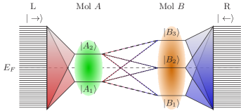
Figure 14: Schematic illustration of two molecules coupled to 2 electrodes. One can follow each of the lines connecting molecule $A$ and $B$. To scatter into the right electrode they have to scatter across the molecular states $|A_{1}\rangle$, $|A_{2}\rangle$, $|B_{1}\rangle$, $|B_{2}\rangle$ and $|B_{3}\rangle$.

As an example of projections based on a realistic DFT-NEGF calculation featuring the $\mathbf{k}$-dependence we consider again transport through a monolayer of $\mathrm{C}_{60}$ molecules as shown in Fig. 15 (setup from Ref. Schneider et al. (2015)). Due to the densely packed monolayer coverage of $\mathrm{C}_{60}$ – one molecule per $4\times 4$-surface area of Cu(111) – there exists a slight dispersion in the Brillouin zone ($\sim 10\,\mathrm{meV}$). The transmissions are calculated on a $13\smash{\times}13$ Monkhorst-Pack grid Monkhorst and Pack (1976). Here we limit the projections to involve the three (almost) degenerate MPSH orbitals close to the Fermi energy $E_{F}$, i.e., essentially to the lowest unoccupied molecular orbitals (LUMO) of $\mathrm{C}_{60}$. The highest occupied molecular orbitals (HOMO) are located about $-1\,\mathrm{eV}$ below $E_{F}$ while the LUMO$+1$ are about $1\,\mathrm{eV}$ above $E_{F}$. In Fig. 15 we compare the full transmission (thick black) with the projected transmissions. Figures in the left column are the $\Gamma$-point projectors used in the entire Brillouin zone, while the right column figures are using the projectors at the given $\mathbf{k}$ in the Brillouin zone. Projections labeled by a single integer are individual MPSH projections, while $1-3$ is the summed projection over all LUMO levels.

The top row of Fig. 15 shows the projected transmissions using the projectors as in Eq. (37c). The relative contributions from the dashed lines clearly reveal that a single LUMO orbital is responsible for carrying the majority of the transmission, while the other two LUMO orbitals have negligible contribution. The full projectors ($1-3$) only slightly increases the total transmission compared to the 3rd projection. The ordering of the levels are according to the energy levels. The total transmission is not reached due to hybridization of the molecule with the electrode. One can also observe the effect of intra-molecular coupling yielding a dispersion in the densely packed monolayer by comparing the results with the $\Gamma$-point versus the $\mathbf{k}$-resolved projectors. The latter projection increases the Lorentzian shape of the transmission peak as well as decrease the hybridized contributions in the energy range corresponding to the HOMO levels, as expected.

The projectors may take either of the forms shown in Eqs. (37). A comparison between these different choices are shown in the lower row of Fig. 15. The hybridization of the $\mathrm{C}_{60}$ molecules with the Cu states is strong as reflected in the many small peaks with the $\rightarrow$ projectors. Contrary, $\leftarrow$ which projects the molecular orbitals through the weakly coupled tip retains the LUMO energy range as well as reducing the Brillouin zone dispersion. The latter proves that we have a small coupling between tips in different supercells resulting in a low dispersion. It can also be seen that the total transmission is better retained when using only $\rightarrow$ or $\leftarrow$ which infers a mixing of the scattering states with the molecular orbitals.

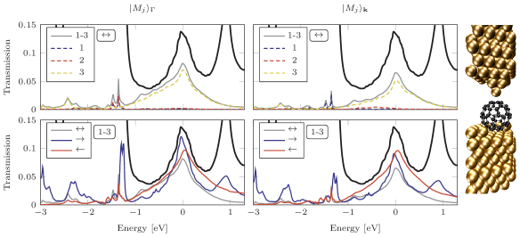
Figure 15: Projected transmission spectra onto the molecular orbitals at zero bias for a Cu(111) surface covered with $\mathrm{C}_{60}$ molecules ($E_{F}=0$ eV). The full black line is the $\mathbf{k}$-sampled total transmission (same curve in all panels). Projections of the essentially 3-fold degenerate LUMO levels are shown with both non-dispersive (left) and dispersive (right) projectors. The in-out projectors are used in the top row, while a comparison of the in/out/in-out projectors are shown in the bottom row. The Brillouin zone dispersion requires the projections to be $\mathbf{k}$-resolved and it is seen that only a single LUMO MPSH is responsible for the majority of the transmission.

IV.6 Phonon transport — phtrans

The tailoring of heat transport in nanostructures (e.g., via nanostructuring of materials) is a topic with a large and growing community following the trend of electronic transport Wang et al. (2008); Dhar (2008). It has promising applications in thermal management and thermoelectrics, and has even been envisioned for information processing with devices, akin of electronics, known as “phononics” Li et al. (2012). The transport of heat via phonons can be treated using the Landauer formula by replacing (from the electronic case) Fermi-distributions with Bose-Einstein distributions Zhang et al. (2007); Yamamoto and Watanabe (2006), carrier charge ($e$) with phonon energy ($\hbar\omega$), and using the phonon transmission function $\Xi(\omega)$. The phonon thermal conductance between two reservoirs at tempertures $T$ and $T+\mathrm{d}T$, can thus be calculated as

$$\kappa_{\mathrm{ph}}(T)=\frac{\hbar^{2}}{2\pi k_{B}T^{2}}\int_{0}^{\infty}\mathrm{d}\omega\,\omega^{2}\,\Xi(\omega)\,\frac{e^{\hbar\omega/k_{B}T}}{(e^{\hbar\omega/k_{B}T}-1)^{2}}.$$ (38)

The expression for the electronic transmission function in Sec. IV is easily converted to that of phonons by replacing the dynamical matrix for the Hamiltonian, using unity as overlap, and the energy replacement, $\varepsilon+i\eta\rightarrow\omega^{2}+i\eta^{2}$. Recall that all tbtrans functionality may be used in phtrans, including $N_{\mathfrak{e}}\geq 1$ terminals. Phonon transport using the Green function formalism can thus be written as

$$\mathbf{G}_{\mathbf{q}}(\omega) =\big{[}(\omega^{2}+i\eta^{2})\mathbf{I}-\mathbf{D}_{\mathbf{q}}-\boldsymbol{\Sigma}_{\mathbf{q}}(\omega)\big{]}^{-1},$$ (39)

$$\Xi_{\mathfrak{e}\mathfrak{e}^{\prime},\mathbf{q}}(\omega) =\operatorname{Tr}\big{[}\mathbf{G}_{\mathbf{q}}(\omega)\boldsymbol{\Gamma}_{\mathfrak{e},\mathbf{q}}\mathbf{G}^{\dagger}_{\mathbf{q}}(\omega)\boldsymbol{\Gamma}_{\mathfrak{e}^{\prime},\mathbf{q}}\big{]},$$ (40)

with $\mathbf{D}_{\mathbf{q}}$ being the dynamical matrix at the $\mathbf{q}$-point in reciprocal space. Currently sisl allows for the extraction of dynamical matrices directly from gulp Gale and Rohl (2003) and outputs files to phtrans compatible data format. This enables the calculation of phonon transport properties for very large systems from empirical potentials using 3rd party tools.

As an example of the capabilities of phtrans we investigated phonon transport in graphene as well as through a grain boundary. Grain boundaries play a significant role for both electronic and heat transport in graphene and is an area of intense research Huang et al. (2011); Yasaei et al. (2015). Figure 16 shows the phonon properties of pristine graphene and the zero-angle grain boundary (GB558, see inset to Fig. 16c) for which the electronic transport has previously been studied Rodrigues et al. (2013). The quantities are calculated using the Brenner potential Brenner et al. (2002) in gulp. The transmission of pristine graphene versus GB558 is compared in Fig. 16a. It is seen how the grain-boundary effectively scatters the phonons and reduces the heat transport to $\sim 60$% at 600K compared to the pristine case (inset Fig. 16a).

Figures 16b,c compare atom-resolved phonon DOS inside pristine graphene and in the grain-boundary, respectively. The grain-boundary hosts quite localized out-of-plane modes around $\hbar\omega=115\,\mathrm{meV}$ and in-plane modes around $\hbar\omega=200\,\mathrm{meV}$ as seen by the peaks in the projected DOS.

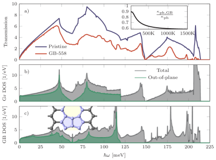
Figure 16: a) Graphene and GB558 (Stone-Wales defect) transmission, $\mathbf{q}$-averaged, for the primitive unit-cell. Insert: Ratio of thermal transmissions as a function of temperature calculated using Eq. (38). b) Total DOS and out-of-plane projected DOS per atom of pristine graphene. c) Total DOS and projected DOS on out-of-plane phonons, projected onto GB-558 atoms. Insert: GB558 structure and projection atoms (blue).

V Conclusions

We have presented the Green function technique and its implementation at the DFT-NEGF level with a generalization of the equations to cover both equilibrium single-electrode ($N_{\mathfrak{e}}=1$) and non-equilibrium multi-electrode ($N_{\mathfrak{e}}>1$) calculations. The first case enables equilibrium surface calculations without resorting to slab-approximations, while the latter case makes studies of non-equilibrium thermo-electric effects possible using independent electrode Fermi distributions (both chemical potentials and temperatures). The methods are made available in the GPL licensed DFT-NEGF code transiesta together with the post-processing electron (phonon) transport code tbtrans (phtrans). Both codes were re-implemented for extended functionality and optimization.

We now summarize the specific major improvements to the method. We have implemented several schemes for equilibrium contour integration to obtain the density matrix. These improve the convergence properties while reducing the number of integration abscissa in the equilibrium contour. Along these lines we generalized the original weighting scheme for the density matrix integrals to the multi-electrode case ($N_{\mathfrak{e}}>2$). Besides the multi-electrode capabilities we have also implemented a flexible way to include charge/Hartree electrostatic gate geometries in the DFT-NEGF device region. This enables investigating gate effects which are ubiquitous for e.g. simulations of functional electronic devices.

The algorithm for calculating the Green function using matrix inversion is crucial for the performance of any DFT-NEGF code. We have compared 3 implemented methods, LAPACK, MUMPS, and BTD inversion. We found that the BDT method performs the best and devised a highly efficient, memory-wise and performance-wise, NEGF variant. The BTD method relies critically on the bandwidth of the matrix to be inverted and to accommodate this, we implemented a variety of pivoting algorithms to reduce bandwidth, memory consumption and increase performance of the NEGF calculation. We have furthermore implemented an efficient method to calculate the spectral function using an efficient propagation algorithm. Altogether, the performance of transiesta has improved drastically, compared to version 3.2, and for one test system an impressive $\sim 100$ times speed-up was achieved. OpenMP 3.1 threading was also implemented in transiesta which allows to reach unprecedented system sizes with the DFT-NEGF method.

As a post-processing tool tbtrans has been presented for calculation of the transmission function from any Hamiltonian or dynamical matrix (phtrans, phonon-transport). Our implementation involves a new separation algorithm where the transport properties — as well as local quantities such as DOS, bond-currents, etc. — may be efficiently calculated in a selected subspace of the device cell. A recurring question within molecular electronics is the origin of the electron carrier orbital. We presented a novel method to calculate projected transmissions using either single molecular orbitals or a combination of several orbitals. The projection method includes $\Gamma$ and $\mathbf{k}$ point projectors.

Besides the many optimizations mentioned above we also implemented an efficient interpolation method of finite-bias Hamiltonians for tbtrans. This reduces the computational burden of full $I-V$ curves. We presented linear and spline interpolation and demonstrated how spline interpolation proves very accurate, even for complex systems. tbtrans is now featured as a stand-alone transport code which enables other codes to interface to it. In particular, we developed sisl which is a generic Python code for creating and manipulating Hamiltonians. sisl can already now interact with several codes as well as extracting the dynamical matrix from gulp and passing it to phtrans.

All together transiesta and tbtrans (and its offshoot phtrans) now utilize highly scalable and efficient algorithms. Both codes fully implement $N_{\mathfrak{e}}\geq 1$ electrode Green function techniques with full customization of each electrode. Our novel implementations have thus enabled everyday DFT-NEGF (tight-binding) calculations in excess of 10,000 (1,000,000) orbitals which earlier would have seemed insurmountable.

VI Acknowledgments

We thank Mads Engelund, Pedro Brandimarte and Georg Huhs for testing and feedback on the software. The DIPC funded an external stay for NP during code development. The Danish e-Infrastructure Cooperation (DeIC) provided computer resources. The Center for Nanostructured Graphene (CNG) is sponsored by the Danish Research Foundation, Project DNRF103. We acknowledge financial support from EU H2020 project no. 676598, “MaX: Materials at the eXascale” Center of Excellence in Supercomputing Applications, the Basque Departamento de Educación and the UPV/EHU (IT-756-13), the Spanish Ministerio de Economía y Competitividad (MAT2013-46593-C6-2-P, MAT2015-66888-C3-2-R, FIS2012-37549-C05-05, and FIS2015-64886-C5-4-P as well as the “Severo Ochoa” Program for Centers of Excellence in R&D SEV-2015-0496), the European Union FP7-ICT project PAMS (Contract No. 610446), and the Generalitat de Catalunya (2014 SGR 301).

References

- Feynman et al. (1965) R. P. R. P. Feynman, R. B. Leighton, and M. L. M. L. Sands, The Feynman lectures on physics (1963–1965).
- SRM (2014) (2014).
- Büttiker et al. (1985) M. Büttiker, Y. Imry, R. Landauer, and S. Pinhas, Phys. Rev. B 31, 6207 (1985).
- Sautet and Joachim (1988) P. Sautet and C. Joachim, Phys. Rev. B 38, 12238 (1988).
- Datta (1997) S. Datta, Electronic Transport in Mesoscopic Systems (Cambridge Studies in Semiconductor Physics and Microelectronic Engineering) (Cambridge University Press, 1997).
- Sanvito et al. (1999) S. Sanvito, C. J. Lambert, J. H. Jefferson, and A. M. Bratkovsky, Phys. Rev. B 59, 11936 (1999).
- Delaney and Greer (2004) P. Delaney and J. C. Greer, Phys. Rev. Lett. 93, 036805 (2004).
- Darancet et al. (2007) P. Darancet, A. Ferretti, D. Mayou, and V. Olevano, Phys. Rev. B 75, 075102 (2007).
- Mirjani and Thijssen (2011a) F. Mirjani and J. M. Thijssen, Phys. Rev. B 83, 035415 (2011a).
- Ness and Dash (2012) H. Ness and L. K. Dash, Journal of Physics A: Mathematical and Theoretical 45, 195301 (2012).
- Martin (2004) R. M. Martin, Electronic Structure. Basic theory and practical methods. (Cambridge University Press, 2004).
- Stefanucci and Almbladh (2004) G. Stefanucci and C.-O. Almbladh, Europhysics Letters (EPL) 67, 14 (2004).
- Ventra and Todorov (2004) M. D. Ventra and T. N. Todorov, Journal of Physics: Condensed Matter 16, 8025 (2004).
- Stefanucci and Kurth (2015) G. Stefanucci and S. Kurth, Nano Letters 15, 8020 (2015).
- Kurth and Stefanucci (2013) S. Kurth and G. Stefanucci, Phys. Rev. Lett. 111, 030601 (2013).
- Mirjani and Thijssen (2011b) F. Mirjani and J. M. Thijssen, Phys. Rev. B 83, 035415 (2011b).
- Schmitteckert and Evers (2008) P. Schmitteckert and F. Evers, Phys. Rev. Lett. 100, 086401 (2008).
- Mera and Niquet (2010) H. Mera and Y. M. Niquet, Phys. Rev. Lett. 105, 216408 (2010).
- Taylor et al. (2001) J. Taylor, H. Guo, and J. Wang, Physical Review B 63, 245407 (2001).
- Brandbyge et al. (2002) M. Brandbyge, J.-L. Mozos, P. Ordejón, J. Taylor, and K. Stokbro, Physical Review B 65, 1 (2002).
- Palacios et al. (2002) J. J. Palacios, A. J. Pérez-Jiménez, E. Louis, E. SanFabián, and J. A. Vergés, Phys. Rev. B 66, 035322 (2002).
- Wortmann et al. (2002) D. Wortmann, H. Ishida, and S. Blügel, Phys. Rev. B 65, 165103 (2002).
- Rocha et al. (2005) A. R. Rocha, V. M. Garcia-Suarez, S. W. Bailey, C. J. Lambert, J. Ferrer, and S. Sanvito, Nature Materials 4, 335 (2005).
- Garcia-Lekue and Wang (2006) A. Garcia-Lekue and L.-W. Wang, Phys. Rev. B 74, 245404 (2006).
- Wohlthat et al. (2007) S. Wohlthat, F. Pauly, J. K. Viljas, J. C. Cuevas, and G. Schön, Phys. Rev. B 76, 075413 (2007).
- Pecchia et al. (2008) A. Pecchia, G. Penazzi, L. Salvucci, and A. Di Carlo, New Journal of Physics 10, 065022 (2008).
- Saha et al. (2009) K. K. Saha, W. Lu, J. Bernholc, and V. Meunier, The Journal of chemical physics 131, 164105 (2009).
- Ozaki et al. (2010) T. Ozaki, K. Nishio, and H. Kino, Physical Review B 81, 035116 (2010).
- Chen et al. (2012) J. Chen, K. S. Thygesen, and K. W. Jacobsen, Physical Review B 85, 155140 (2012), 1204.4175 .
- Bagrets (2013) A. Bagrets, Journal of Chemical Theory and Computation 9, 2801 (2013).
- Soler et al. (2002) J. M. Soler, E. Artacho, J. D. Gale, A. García, J. Junquera, P. Ordejón, and D. Sánchez-Portal, Journal of Physics: Condensed Matter 14, 2745 (2002).
- Palsgaard et al. (2015) M. L. N. Palsgaard, N. P. Andersen, and M. Brandbyge, Physical Review B 91 (2015), 10.1103/PhysRevB.91.121403.
- Jacobsen et al. (2016) K. W. Jacobsen, J. T. Falkenberg, N. Papior, P. Bøggild, A.-P. Jauho, and M. Brandbyge, Carbon (2016), 10.1016/j.carbon.2016.01.084, arXiv:1601.07708v1 .
- Di Ventra and Pantelides (2000) M. Di Ventra and S. T. Pantelides, Physical Review B 61, 16207 (2000).
- Brandbyge et al. (2003) M. Brandbyge, K. Stokbro, J. Taylor, J.-L. Mozos, and P. Ordejón, Phys. Rev. B 67, 193104 (2003).
- Takahasi and Mori (1974) H. Takahasi and M. Mori, Publications of the Research Institute for Mathematical Sciences 9, 721 (1974).
- Note (1) This is due to the constant DOS for the lower energy part of the contour where the circle is far below the lowest lying eigenvalue and far in the complex plane.
- Li et al. (2007) R. Li, J. Zhang, S. Hou, Z. Qian, Z. Shen, X. Zhao, and Z. Xue, Chemical Physics 336, 127 (2007).
- Amestoy et al. (2000) P. Amestoy, I. Duff, and J.-Y. L’Excellent, Computer Methods in Applied Mechanics and Engineering 184, 501 (2000).
- Amestoy et al. (2001) P. R. Amestoy, I. S. Duff, J.-Y. L’Excellent, and J. Koster, SIAM Journal on Matrix Analysis and Applications 23, 15 (2001).
- Petersen et al. (2008) D. E. Petersen, H. H. B. Sørensen, P. C. Hansen, S. Skelboe, and K. Stokbro, Journal of Computational Physics 227, 3174 (2008).
- Lin et al. (2009) L. Lin, J. Lu, L. Ying, R. Car, and W. E, Comm. Math. Sci. 7, 755 (2009).
- Li et al. (2008) S. Li, S. Ahmed, G. Klimeck, and E. Darve, Journal of Computational Physics 227, 9408 (2008).
- Lin et al. (2011a) L. Lin, C. Yang, J. Lu, L. Ying, and W. E, SIAM Journal on Scientific Computing 33, 1329 (2011a).
- Lin et al. (2011b) L. Lin, C. Yang, J. C. Meza, J. Lu, L. Ying, and W. E, ACM Transactions on Mathematical Software 37, 1 (2011b).
- Jacquelin et al. (2014) M. Jacquelin, L. Lin, and C. Yang, (2014), arXiv:1404.0447 .
- Jacquelin et al. (2015) M. Jacquelin, L. Lin, N. Wichmann, and C. Yang, (2015), arXiv:1504.04714 .
- Hetmaniuk et al. (2013) U. Hetmaniuk, Y. Zhao, and M. Anantram, International Journal for Numerical Methods in Engineering 95, 587 (2013).
- Okuno and Ozaki (2013) Y. Okuno and T. Ozaki, Journal of Physical Chemistry C 117, 100 (2013).
- Feldman et al. (2014) B. Feldman, T. Seideman, O. Hod, and L. Kronik, Phys. Rev. B 90, 035445 (2014).
- Thorgilsson et al. (2014) G. Thorgilsson, G. Viktorsson, and S. Erlingsson, Journal of Computational Physics 261, 256 (2014).
- Anderson et al. (1999) E. Anderson, Z. Bai, C. Bischof, S. Blackford, J. Demmel, J. Dongarra, J. Du Croz, A. Greenbaum, S. Hammarling, A. McKenney, and D. Sorensen, LAPACK Users’ Guide, 3rd ed. (Society for Industrial and Applied Mathematics, 1999).
- Godfrin (1991) E. M. Godfrin, Journal of Physics: Condensed Matter 3, 7843 (1991).
- Hod et al. (2006) O. Hod, J. E. Peralta, and G. E. Scuseria, Journal of Chemical Physics 125 (2006), 10.1063/1.2349482.
- Reuter and Hill (2012) M. G. Reuter and J. C. Hill, Computational Science & Discovery 5, 014009 (2012).
- Note (2) One may solve a set of linear equations: and .
- Note (3) can maximally be split in two consecutive blocks as it is a dense matrix.
- Cuthill and McKee (1969) E. Cuthill and J. McKee, in ACM Proceedings of the 1969 24th national conference (ACM Press, New York, New York, USA, 1969) pp. 157–172.
- Gibbs et al. (1976) N. Gibbs, J. Poole, W.G, and P. Stockmeyer, SIAM Numerical Analysis 2, 236 (1976).
- Wang et al. (2009) Q. Wang, Y.-C. Guo, and X.-W. Shi, Progress In Electromagnetics Research 90, 121 (2009).
- Note (4) A comparison for larger systems is not possible due to transiesta 3.2 Brandbyge et al. (2002) memory consumption.
- Note (5) The MUMPS comparison is thus not justifying the actual performance for large systems.
- Note (6) In siesta threading has only been implemented in a few places, with priority on grid operations.
- Note (7) We have used OpenBLAS 0.2.15 with OpenMP threading using the GNU 5.2.0 compiler for a graphene test system. We use a non-threaded LAPACK. High compiler optimizations are used.
- Rocha et al. (2006) A. R. Rocha, V. M. García-Suarez, S. Bailey, C. Lambert, J. Ferrer, and S. Sanvito, Phys. Rev. B 73, 085414 (2006).
- Papior et al. (2016) N. Papior, T. Gunst, D. Stradi, and M. Brandbyge, Phys. Chem. Chem. Phys. 18, 1025 (2016).
- ATK (2014) “Atomistix ToolKit version 2014.3,” (2014).
- Otani and Sugino (2006) M. Otani and O. Sugino, Physical Review B 73, 115407 (2006).
- Brumme et al. (2014) T. Brumme, M. Calandra, and F. Mauri, Physical Review B 89, 1 (2014).
- Ohta et al. (2007) T. Ohta, A. Bostwick, J. McChesney, T. Seyller, K. Horn, and E. Rotenberg, Physical Review Letters 98, 206802 (2007).
- Engelund et al. (2016) M. Engelund, N. R. Papior, T. Frederiksen, A. García-Lekue, and D. Sánchez-Portal, (2016).
- Johannsen et al. (2013) J. C. Johannsen, S. Ulstrup, F. Cilento, A. Crepaldi, M. Zacchigna, C. Cacho, I. C. E. Turcu, E. Springate, F. Fromm, C. Raidel, T. Seyller, F. Parmigiani, M. Grioni, and P. Hofmann, Physical Review Letters 111, 027403 (2013).
- Gierz et al. (2013) I. Gierz, J. C. Petersen, M. Mitrano, C. Cacho, I. C. E. Turcu, E. Springate, A. Stöhr, A. Köhler, U. Starke, and A. Cavalleri, Nat Mater 12, 1119 (2013).
- Todorov (2002) T. N. Todorov, Journal of Physics: Condensed Matter 14, 3049 (2002).
- Mason et al. (2011) D. J. Mason, D. Prendergast, J. B. Neaton, and E. J. Heller, Physical Review B 84, 155401 (2011).
- Ferrer et al. (2014) J. Ferrer, C. J. Lambert, V. M. García-Suárez, D. Z. Manrique, D. Visontai, L. Oroszlany, R. Rodríguez-Ferradás, I. Grace, S. W. D. Bailey, K. Gillemot, H. Sadeghi, and L. a. Algharagholy, New Journal of Physics 16, 093029 (2014).
- Fisher and Lee (1981) D. S. Fisher and P. A. Lee, Phys. Rev. B 23, 6851 (1981).
- Yeyati and Büttiker (2000) A. L. Yeyati and M. Büttiker, Phys. Rev. B 62, 7307 (2000).
- Lippmann and Schwinger (1950) B. A. Lippmann and J. Schwinger, Physical Review 79, 469 (1950).
- Cook et al. (2011) B. G. Cook, P. Dignard, and K. Varga, Physical Review B 83, 205105 (2011).
- Lake et al. (1997) R. Lake, G. Klimeck, R. C. Bowen, and D. Jovanovic, Journal of Applied Physics 81, 7845 (1997).
- Note (8) Typically this is a problem for systems with relatively large bulk transmissions compared to the transmission. If the number of incoming channels are only a couple of magnitude orders larger than the transmission the numerical precision is adequate.
- Paulsson and Brandbyge (2007) M. Paulsson and M. Brandbyge, Physical Review B 76, 1 (2007).
- Schneider et al. (2012) N. L. Schneider, J. T. Lü, M. Brandbyge, and R. Berndt, Physical Review Letters 109, 186601 (2012).
- Falkenberg and Brandbyge (2015) J. T. Falkenberg and M. Brandbyge, Beilstein Journal of Nanotechnology 6, 1603 (2015), arXiv:1505.03267 .
- Schneider et al. (2015) N. L. Schneider, N. Néel, N. P. Andersen, J. T. Lü, M. Brandbyge, J. Kröger, and R. Berndt, Journal of Physics: Condensed Matter 27, 015001 (2015).
- Papior (2016) N. R. Papior, “sisl: 0.7.1,” (2016).
- Gale and Rohl (2003) J. D. Gale and A. L. Rohl, Molecular Simulation 29, 291 (2003).
- Mostofi et al. (2014) A. A. Mostofi, J. R. Yates, G. Pizzi, Y.-S. Lee, I. Souza, D. Vanderbilt, and N. Marzari, Computer Physics Communications 185, 2309 (2014).
- Hancock et al. (2010) Y. Hancock, A. Uppstu, K. Saloriutta, A. Harju, and M. J. Puska, Physical Review B 81, 245402 (2010).
- García-Suárez and Lambert (2011) V. M. García-Suárez and C. J. Lambert, New Journal of Physics 13 (2011), 10.1088/1367-2630/13/5/053026, arXiv:1101.2778 .
- Solomon et al. (2010) G. C. Solomon, C. Herrmann, T. Hansen, V. Mujica, and M. A. Ratner, Nat Chem 2, 223 (2010).
- Stokbro et al. (2003) K. Stokbro, J. Taylor, M. Brandbyge, J. L. Mozos, and P. Ordejón, Comput. Mater. Sci. 27, 151 (2003).
- Löwdin (1950) P.-O. Löwdin, The Journal of Chemical Physics 18, 365 (1950).
- Rangel et al. (2015) T. Rangel, G.-M. Rignanese, and V. Olevano, Beilstein Journal of Nanotechnology 6, 1247 (2015).
- Monkhorst and Pack (1976) H. J. Monkhorst and J. D. Pack, Physical Review B 13, 5188 (1976).
- Wang et al. (2008) J.-S. Wang, J. Wang, and T. J. Lü, The European Physical Journal B 62, 381 (2008).
- Dhar (2008) A. Dhar, Advances in Physics 57, 457 (2008).
- Li et al. (2012) N. Li, J. Ren, L. Wang, G. Zhang, P. Hänggi, and B. Li, Reviews of Modern Physics 84, 1045 (2012).
- Zhang et al. (2007) W. Zhang, T. S. Fisher, and N. Mingo, Numer. Heat Transf. Part B Fundam. 51, 333 (2007).
- Yamamoto and Watanabe (2006) T. Yamamoto and K. Watanabe, Physical Review Letters 96, 255503 (2006).
- Huang et al. (2011) P. Y. Huang, C. S. Ruiz-Vargas, A. M. van der Zande, W. S. Whitney, M. P. Levendorf, J. W. Kevek, S. Garg, J. S. Alden, C. J. Hustedt, Y. Zhu, J. Park, P. L. McEuen, and D. A. Muller, Nature 469, 389 (2011).
- Yasaei et al. (2015) P. Yasaei, A. Fathizadeh, R. Hantehzadeh, A. K. Majee, A. El-Ghandour, D. Estrada, C. Foster, Z. Aksamija, F. Khalili-Araghi, and A. Salehi-Khojin, Nano Lett. 15, 4532 (2015).
- Rodrigues et al. (2013) J. N. B. Rodrigues, N. M. R. Peres, and J. M. B. Lopes dos Santos, J. Phys. Condens. Matter 25, 075303 (2013).
- Brenner et al. (2002) D. W. Brenner, O. a. Shenderova, J. a. Harrison, S. J. Stuart, B. Ni, and S. B. Sinnott, J. Phys. Condens. Matter 14, 783 (2002).