Normal modes of a superconducting transmission-line resonator with embedded lumped element circuit components

Abstract

We present a method to identify the coupled, normal modes of a superconducting transmission-line with an embedded lumped element circuit. We evaluate the effective transmission-line non-linearities in the case of Kerr-like Josephson interactions in the circuit and in the case where the embedded circuit constitutes a qubit degree of freedom, which is Rabi coupled to the field in the transmission-line. Our theory quantitatively accounts for the very high and positive Kerr non-linearities observed in a recent experiment [M. Rehák et.al., Appl. Phys. Lett. 104, 162604], and we can evaluate the accomplishments of modified versions of the experimental circuit.

I Introduction

The quantum mechanical interaction between light and matter is of major importance in non-linear optics and quantum optics. Recently, the field of circuit QED Wallraff et al. (2004); Blais et al. (2004) has seen immense progress with superconducting circuits playing the role of artificial atoms which can interact with confined microwave photons and produce quantum optical effects such as vacuum Rabi-splitting Wallraff et al. (2004); Abdumalikov Jr et al. (2008), parametric amplification Castellanos-Beltran et al. (2008); Hatridge et al. (2011); Rehák et al. (2014), single atom lasing Astafiev et al. (2007); Neilinger et al. (2015), and photon-mediated interactions Van Loo et al. (2013). The photonic non-linearity of these experiments arises from the non-linear interactions in Josephson junctions in the superconducting circuits which are embedded in microwave transmission-line waveguides and resonator architectures.

Linear, classical microwave circuits can be fully characterized by their impedance Pozar (2009) which, e.g., reveals their transmission properties and resonances. The quantum description follows in a similar manner Nigg et al. (2012), and a transmission-line resonator can thus be described by its classical eigenmodes which directly translate into a quantum Hamiltonian as a sum of harmonic oscillators. Josephson junctions, on the other hand, are non-linear elements, i.e., they are not described as harmonic oscillators and their incorporation in circuit architectures causes non-linear and potentially non-classical quantum effects. A single Josephson junction is described by an energy potential which is a cosine function of the quantum mechanical phase variable. If the cosine potential is deep and supports many eigenstates, we can expand the potential and obtain an effective Kerr-effect in our system Bourassa et al. (2012); Leib et al. (2012); Eichler and Wallraff (2014); Nigg et al. (2012), while if it supports only few eigenstates with irregular level spacing, the dynamics may be restricted to the two lowest eigenstates which constitute a single qubit Nakamura et al. (1999). By shunting the Josephson junction with a large capacitor and coupling it capacitively to a resonator or by adding several Josephson junctions in a superconducting loop, one can obtain the so-called transmon qubits Koch et al. (2007) or flux qubits Mooij et al. (1999); Yan et al. (2015).

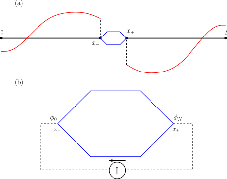
Figure 1: (a) Schematic drawing of an inline lumped element circuit (blue) which introduces a boundary value discontinuity in the mode envelopes of a transmission-line (red) and hence perturbs both the eigenfrequencies and the coupling strengths compared to the bare mode case. (b) The transmission-line is modeled as a current source to the inner circuit, with the current given by the transmission-line flux variable

As illustrated in Fig. 1 (a), when small quantum circuit systems are embedded in waveguide resonators, they enforce local boundary conditions on the transmission-line variables, and they may hence not only interact with but also significantly modify the waveguide mode structure. In this work we will present a general approach to describe the linear eigenmodes of an arbitrary circuit embedded in a transmission-line resonator. The eigenmodes of the coupled systems are then taken as the basis for the pertubative inclusion of non-linear interactions. Our approach builds on the Lagrangian formalism Devoret (1995); Yurke and Denker (1984) and it generalizes prior approaches used to describe weakly non-linear systems Bourassa et al. (2012); Weißl et al. (2015); Leib et al. (2012); Leib and Hartmann (2014) applied, e.g., as microwave amplifiers Eichler and Wallraff (2014); Eichler et al. (2014). Motivated by a recent experiment Rehák et al. (2014) that used a pair of flux qubits inside a resonator for parametric amplification, we will extend our formalism to specifically deal with flux qubits in the system.

The article is organized as follows: In Sec. II we review the general spanning tree method to deal with lumped element circuit and with waveguide components, and we identify the normal modes of a resonator with an arbitrary embedded circuit and their quantum mechanical and non-linear interactions. Section III deals with the inclusion of a strongly coupled flux qubits which causes Rabi splitting of the mode structure and which cannot be described directly by a perturbative Kerr-interaction. In Sec. IV we apply our formalism to a recent experiment and in Sec. V, we conclude and provide an outlook.

II Coupling a discrete circuit with a continuous mode

Standard techniques exists to quantize the modes of a resonator Blais et al. (2004) and the degrees of freedom of coupled, lumped element superconducting circuits Devoret (1995). The combination of a discrete circuit and a resonator mode has also been considered in special cases Blais et al. (2004); Bourassa et al. (2012); Andersen and Mølmer (2015), but without establishing a general framework. In this section, we use the standard nodal technique to provide such a general, practical theory as a generalization of the method in Ref. Bourassa et al. (2012).

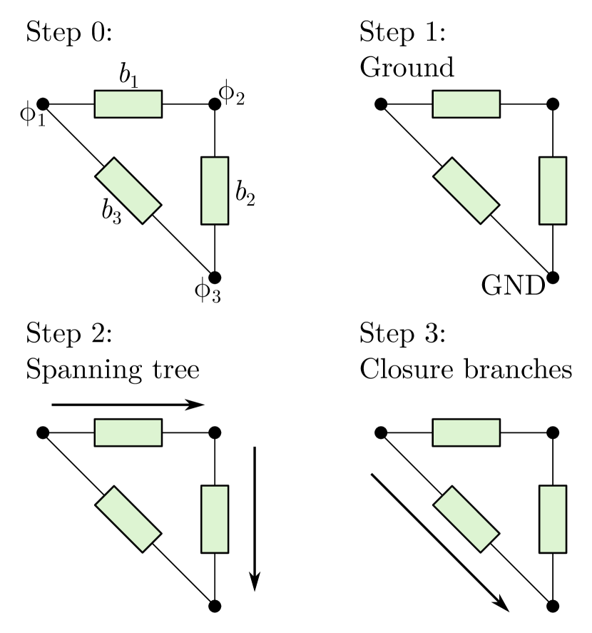
Figure 2: The steps required to analyze an arbitrary network. For illustrative purposes we have in step 0 three nodes, $\phi_{n}$, connected by the branches $b_{i}$. The branches can be either inductive or capacitive elements. The first step is to define a ground node, here the node $\phi_{3}$. Then in step 2, we choose a spanning tree, $b_{1}$ and $b_{2}$, with a given direction, which defines a positive direction of a voltage drop. Then finally we identify the closure branches and their direction, here only $b_{3}$.

Well-suited coordinates for a Lagrangian description of circuit electron dynamics Devoret (1995) are the so-called node flux variables $\phi_{n}(t)$, given as the time-integral of the voltage at different nodes in the circuit. A complete, consistent description of all $N$ nodes of a circuit is given by considering the inductor and capacitor elements connecting the nodes as branches and choosing a spanning tree of paths such that every node is reached from a chosen reference (ground) node through only one path. The rest of the branches are then referred to as closure branches. This approach is sketched in Fig. 2 and following these steps takes care of the gauge degree of freedom in analyzing electrical circuits Devoret (1995). Let $\delta_{m}$ denote the time-integral of the voltage difference, the branch flux, across each branch element. The flux variables $\phi_{n}(t)$ are then given by the sum of the branch fluxes along the path connecting the nodes to ground, and it can, in turn be written as a sum over all branch fluxes

$$\phi_{n}(t)=\sum_{b}S_{nb}\delta_{b}(t),$$ (1)

where the factors $S_{nb}=\pm 1$ if the branch $b$ is in the path towards the node $n$, with the sign $+(-)$ depending on the voltage difference being defined towards (away from) the node, and $S_{nb}=0$ if $b$ is not in the path connecting the node $n$ to the ground node. With the node description in place, we obtain the transformation from node to branch variables coming from all $S_{nb}$,

$${\delta}(t)=\mathbf{K}\vec{\phi}(t),$$ (2)

where $\mathbf{K}$ is the the incidence matrix,

$$\mathbf{K}_{ij}=\Bigg{\{}\begin{array}[]{lr}1&\text{if branch $i$ has node $j$ at the + end}\\ -1&\text{if branch $i$ has node $j$ at the - end}\\ 0&\text{otherwise},\end{array}$$ (3)

and the variables $\delta(t)$ and $\vec{\phi}(t)$ are vectors containing all $\delta_{n}$ and $\phi_{n}$, respectively. We remark that, the matrix $K$ is uniquely defined once the steps of Fig. 2 are followed.

For a circuit whose branches are only inductors and capacitors we define the following matrices in the basis of branch variables,

$$\mathbf{L} =\text{diag}\{1/L_{1},\dots,1/L_{M}\}$$ (4)

$$\mathbf{C} =\text{diag}\{C_{1},\dots,C_{M}\},$$ (5)

where $L_{i}$ and $C_{i}$ are the inductance and capacitance of branch $i$ (replace $1/L_{i}$ with 0 if the inductance of the $i$th branch is zero). The Lagrangian description of the circuit is obtained by treating inductive energy, $E_{L}=\delta/2L$, and capacitive energy, $E_{C}=C\partial_{t}\delta/2$, as potential and kinetic energy respectively, and using Eq. (2) to transform from flux to branch variables,

$$\mathcal{L}_{lin}\left(\vec{\phi}(t),\partial_{t}\vec{\phi}(t)\right)=\frac{1}{2}\partial_{t}\vec{\phi}(t)^{\text{T}}{}\tilde{\mathbf{C}}\hskip 1.0pt\partial_{t}\vec{\phi}(t)+\frac{1}{2}\vec{\phi}(t)^{\text{T}}{}\tilde{\mathbf{L}}\vec{\phi}(t),$$ (6)

with $\tilde{\mathbf{C}}=\mathbf{K}^{\text{T}}{}\mathbf{C}\mathbf{K}$ and $\tilde{\mathbf{L}}=\mathbf{K}^{\text{T}}{}\mathbf{L}\mathbf{K}$. This Lagrangian yields the equations of motion for the flux variables

$$\tilde{\mathbf{C}}\partial_{t}^{2}{\vec{\phi}}(t)+\tilde{\mathbf{L}}\vec{\phi}(t)=0,$$ (7)

which is automatically equivalent the Kirchoff equations for the circuit Devoret (1995).

With the above giving an appropriate description for a discrete lumped element circuit, we need also to consider distributed elements such as a transmission-line resonator as our goal is to combine the two. A transmission-line can be considered as a series of LC-circuits of length $\Delta x$. In the limit $\Delta x\rightarrow 0$, the flux at each node becomes a continuous function, which we for convenience will denote $\psi(x,t)$, but it plays the same role as $\vec{\phi}(t)$ in the discrete case. Treating the transmission-line first as a lumped element circuit, we can obtain an equation of motion on the form of Eq. (7). For a series of $LC$-circuits the corresponding matrix $K$ connects each node with both neighboring nodes which generates inductive energy leading to terms of the form $(2\psi_{n}-\psi_{n+1}-\psi_{n-1})/\Delta x^{2}$ in the equation of motion. This is equivalent to the curvature of a continuous function when taking the continuum limit and the equation of motion emerges as the wave equation,

$$\partial_{t}^{2}\psi(x,t)-v^{2}\partial_{x}^{2}\psi(x,t)=0,$$ (8)

with $v=\sqrt{1/L_{0}C_{0}}$ with $L_{0}$ and $C_{0}$ being the inductance and capacitance per length of the transmission-line. Notice, that the current in the transmission-line is given by

$$I(x,t)=-\frac{1}{L_{0}}\partial_{x}\psi(x,t).$$ (9)

II.1 Normal modes of the combined system, linear theory

For a finite transmission-line resonator embedded with a linear lumped element circuit, the dynamics of the combined system can be described in terms of common normal modes for the full system. Such normal modes consist of both a continuous and a discrete part which we now will denote $\psi_{m}(x,t)$ and $\vec{\phi}_{m}(t)$ respectively and both are oscillating at a common angular frequency $\omega_{m}$. However, the functions, $\psi_{m}$ and $\vec{\phi}_{m}$, depend on $\omega_{m}$ and must by found by solving one combined eigenvalue problem including both the discrete and the continuous part. The aim of this section is therefore to formulate such an eigenvalue problem.

For the frequencies of interest, the spatial solutions of the continuous wave equation along the transmission-line vary on the length scale $l$ of centimeters, while the lumped circuits are much smaller and described by discrete flux variables. The inline circuit thus introduces an effectively discontinuous drop in the transmission-line flux, $\Delta\psi$, across the embedded circuit Bourassa et al. (2012) (see Fig. 1 (a)). For each normal mode, we therefore define

$$\Delta\psi_{m}(t)=\psi_{m}(x_{+},t)-\psi_{m}(x_{-},t).$$ (10)

The spatial transmission-line components of the system eigenmodes further satisfy boundary conditions at $x=0$ and $x=l$, while accommodating also the flux drop at $x=x_{\pm}$.

To calculate $\Delta\psi_{m}(t)$, we treat the transmission-line as a current source for the inline circuit, see Fig. 1 (b). Therefore to diagonalize the system and thus find $\psi_{m}$ and $\vec{\phi}_{m}$ and their appropriate $\omega_{m}$, the Euler-Lagrange equation, Eq. (7), with an extra current drive must be solved together with wave-equation for the transmission line resonator. Restricted to the discrete flux variables, the eigenmode equations are thus given by

$$(\tilde{\mathbf{L}}-\omega_{m}^{2}\tilde{\mathbf{C}})\phi_{m}(t)=\vec{I}_{m}(t).$$ (11)

with the vector of driving currents,

$$\vec{I}_{m}(t)=\begin{pmatrix}-I_{0}(t)\\ 0\\ \vdots\\ 0\\ I_{N}(t)\end{pmatrix}.$$ (12)

where the two current terms represent the resonator mode driving of the node 0 and the node $N$ flux variables. The eigenmode equation, Eq. (11), has a pole at the eigenfrequencies of the inner circuit, but since we are interested in the dressed resonator modes this is not a problem. Therefore, provided the eigenfrequency $\omega_{m}$ is not an eigenfrequency of the isolated inline circuit, the inhomogeneous equation, Eq. (11), is solved by inversion,

$$\vec{\phi}_{m}(t)=\text{inv}(\tilde{\mathbf{L}}-\omega_{m}^{2}\tilde{\mathbf{C}})\cdot\vec{I}_{m}(t).$$ (13)

Now, we can apply the relation between the currents and the derivative of the transmission-line flux $I_{0}=\partial_{x}\psi(x_{-})/L_{0}=I_{N}=\partial_{x}\psi(x_{+})/L_{0}$. The transmission-line flux drop across the circuit is given by the flux at the 0th and $N$th node (at $x_{-}$ and $x_{+}$), therefore, combining Eq. (13) with Eq. (10) we obtain the equation

$$\Delta\psi_{m}(t) =\text{inv}(\tilde{\mathbf{L}}-\omega_{m}^{2}\tilde{\mathbf{C}})_{0,0}\hskip 1.0ptI_{0}(t)$$

$$\quad-\text{inv}(\tilde{\mathbf{L}}-\omega_{m}^{2}\tilde{\mathbf{C}})_{0,N}\hskip 1.0ptI_{N}(t)$$

$$\quad-\text{inv}(\tilde{\mathbf{L}}-\omega_{m}^{2}\tilde{\mathbf{C}})_{N,0}\hskip 1.0ptI_{0}(t)$$

$$\quad+\text{inv}(\tilde{\mathbf{L}}-\omega_{m}^{2}\tilde{\mathbf{C}})_{N,N}\hskip 1.0ptI_{N}(t).$$ (14)

As alluded to earlier, this equation must be solved together with the wave equation, Eq. (8), which has the normal mode solutions $\psi_{m}(x)\propto\cos(k_{\omega_{m}}x+\phi_{m}^{\pm})$. Here we have $k_{\omega_{m}}\propto\omega_{m}$ as the wave number and $\phi_{m}^{\pm}$ the flux set by the boundary conditions at $0$ and $l$, where we use $\pm$ to note the flux for $x$ smaller or larger than $x_{\pm}$. Therefore, the self-consistent solution of the wave equation solution and Eq. (II.1) yield a transcendental equation for $\omega_{m}$.

The combined continuous and discrete modes are orthogonal under the energy inner products Taylor (2005),

$$\braket{\{\psi_{m},\phi_{m}\},\{\psi_{n},\phi_{n}\}}_{C} =C_{0}\int_{\text{TL}}dx\psi_{m}(x)\psi_{n}(x)$$

$$\quad+\phi_{m}^{\text{T}}{}\tilde{C}\phi_{n}$$

$$=C_{\Sigma}\delta_{nm}$$ (15)

$$\braket{\{\psi_{m},\phi_{m}\},\{\psi_{n},\phi_{n}\}}_{L} =\frac{1}{L_{0}}\int_{\text{TL}}dx\partial_{x}\psi_{m}(x)\partial_{x}\psi_{n}(x)$$

$$\quad+\vec{\phi}_{m}^{\text{T}}{}\tilde{L}\vec{\phi}_{n}$$

$$=\frac{1}{L_{\Sigma}^{m}}\delta_{nm}.$$ (16)

Equation (II.1) and Eq. (16) enable the diagonalization of the full Lagrangian, given by Eq. (6) and $\mathcal{L}_{tl}=\int_{0}^{l}\frac{C_{0}}{2}(\partial_{t}\psi)^{2}+\frac{1}{2L_{0}}(\partial_{x}\psi)^{2}dx$. Fixing the normalization of $\psi_{m}$ and $\phi_{m}$ by Eq. (II.1) we obtain $\omega_{m}=1/\sqrt{C_{\Sigma}^{\phantom{m}}L_{\Sigma}^{m}}$.

II.2 Quantization of the system

With the normal modes obtained by solving Eq. (II.1) together with Eq. (8) and (13), we write a harmonically varying eigensolution as

$$\varphi_{m}(x,t)=\varphi_{m}(t)u_{m}(x)$$ (17)

with $x\in\{[0;l],0,1,\ldots,N\}$. Here, the stationary mode function $u_{m}(x)$

$$u_{m}(x)=\begin{cases}\psi_{m}(x)&\text{ if }x\in[0;l]\\ \vec{e}_{x}^{\;\text{T}}\vec{\phi}_{m}&\text{ if }x\in\{0,1,\ldots N\}\end{cases}$$ (18)

with $\vec{e}_{x}$ being the $x$th unit vector, satisfies the normalization given by Eq. (II.1). $\varphi_{m}(t)$ is the time dependent amplitude with the canonically conjugate variable $q_{m}=\partial\mathcal{L}/\partial(\partial_{t}\varphi_{m})$.

We quantize the system by imposing the operator commutator $[\hat{\varphi}_{m},\hat{q}_{m}]=i\hbar$. For convenience, we introduce the annihilation and creation operators $a_{m}$ and $a_{m}^{\dagger}$ as

$$\hat{\varphi}_{m}=\sqrt{\frac{\hbar}{2C_{\Sigma}\omega_{m}}}(a_{m}^{\dagger}+a_{m}),$$ (19)

$$\hat{q}_{m}=i\sqrt{\frac{\hbar}{2C_{\Sigma}\omega_{m}}}(a_{m}^{\dagger}-a_{m}).$$ (20)

and we transform the Lagrangian into a sum of harmonic oscillator Hamiltonians

$$H_{0}=\sum_{m}\hbar\omega_{m}a_{m}^{\dagger}a_{m}^{\phantom{\dagger}}.$$ (21)

II.3 Josephson non-linearity

So far, we considered systems containing only linear elements such as capacitors and inductors, leading to harmonic eigenmodes. These solutions are modified and the dynamics changes when Josephson junctions are introduced, with the characteristic anharmonic Josephson energy,

$$E_{J}(\delta(t)) =E_{J}\cos\left(\frac{2\pi}{\Phi_{0}}\delta(t)\right)$$ (22)

$$=E_{J}-\frac{\delta(t)^{2}}{L_{J}}+\mathcal{O}(\delta(t)^{4})$$ (23)

where $1/L_{J}=(2\pi/\Phi_{0})^{2}E_{J}$ sets the Josephson inductance, $\delta(t)$ is the flux drop across the junction and $\Phi_{0}$ the magnetic flux quantum. For the treatment in this work, $\delta(t)$ will be proportional with the phase drop over the full inner circuit, $\Delta\psi$, and is calculated from $\vec{\phi}$. If the Josephson non-linearity is weak, the linear behaviour of the Josephson Junction can modelled by a capacitor and inductor in parallel and the expansion in the second line of (23) can be directly incorporated in the harmonic oscillator eigenmode description. In this section, we proceed and consider the next term in Eq. (23), yielding a higher order correction to the Hamiltonian

$$H_{\text{nl}}=-\sum_{i\in\{JJ\}}\frac{2\pi^{4}}{3\Phi_{0}^{4}}E_{J,i}(\hat{\delta}_{i})^{4},$$ (24)

where $\hat{\delta}_{i}$ is set as in Eq. (2) and the summation is over all Josephson junctions in the circuit embedded in the transmission-line. This way of re-introducing the higher order terms is only valid if the energy associated with the non-linear part is much smaller than $\hbar\omega_{m}$ Bourassa et al. (2012); Nigg et al. (2012). Expanding the operator expression on the eigenmode creation and annihilaton operators,cf., Eq. (19), and keeping only the energy preserving Kerr-like terms, we obtain the Hamiltonian

$$H_{\text{nl}}=\sum_{m,n}\frac{\hbar K_{mn}}{2}(a_{m}^{\dagger}a_{m}a_{n}^{\dagger}a_{n}+a_{m}^{\dagger}a_{m})$$ (25)

with

$$K_{mm}=-\sum_{i\in\{JJ\}}\frac{\pi^{4}\hbar}{\Phi_{0}^{4}}\frac{E_{j,i}}{C_{\Sigma}^{2}\omega_{m}^{2}}\Delta u_{m,i}^{4}$$ (26)

with $\Delta u_{m,i}$ denoting the difference in the normalized eigenmode function $u_{m}$ over the $i$th Josephson junction and similarly we find $K_{mn}=-2\sqrt{K_{nn}K_{mm}}$.

By finding the consistent eigenmodes and their eigenfrequencies, which may differ significantly from the bare transmission-line resonances, we have taken the linear couplings in the systems fully into account, and we have effectively treated the higher order non-linear terms as a perturbation. This perturbation affects the amplitude and population dynamics of the modes but not their spatiotemporal character. The Kerr-like field interaction (26) thus leads to a number of quantum optical effects, while cross-Kerr effects, via $K_{mn}$ represent dispersive interactions between the field and the circuit degrees of freedom or among the latter. In the following section, we shall deal with cases, where a different procedure is necessary because the non-linear coupling significantly affects the mode structure.

III Coupling to a flux qubit

For flux qubits, Josephson Junctions are contained within a closed loop in the circuit. In the linear regime, currents in such loops constitute additional internal modes that cannot be identified with Eq. (II.1) and do not couple to the transmission-line, and they are thus not relevant for the dynamics of the normal modes found above. Due to the non-linearity of the Josephson elements, these modes may, however, couple strongly to other modes. In particular, if an embedded loop constitutes a qubit degree of freedom we may obtain a Jaynes-Cummings like coupling between the qubit and the transmission-line mode, which, in turn, can lead to a Rabi-splitting of the modes – a highly nonlinear effect not captured by the perturbative Kerr terms. Therefore, we need to find the resonator modes using the method of Sec. II and combine it with a proper description of the qubit degrees of freedom.

To illustrate this and provide a method to deal with the quantum dynamics of such systems, we consider a flux qubit consisting of a superconducting loop with three (or more) Josephson junctions. Following the treatment of Bourassa et.al Bourassa et al. (2009) we write the Lagrangian for the flux qubit as

$$\mathcal{L}_{fq}=\sum_{k=1}^{3}\bigg{[}\frac{C_{J,k}}{2}\dot{\phi}_{k}^{2}+E_{J,k}\cos(2\pi\phi_{k}/\Phi_{0})\bigg{]}$$ (27)

with $k$ summing over the three junctions. The junctions 1 and 3 are identical with $C_{J,1}=C_{J,3}=C_{J}$ and $E_{J,1}=E_{J,3}=E_{J}$, while the center junction 2, referred to as the $\alpha$-junction, has $E_{J,2}=\alpha E_{J}$ and $C_{J,2}=\alpha C_{J}$ with $\alpha<1$. Note that the inner circuit may have further capacitors that contribute both to the overall energy of the qubit and to the coupling with the resonator. The charge coupling to the resonator is typically weak for flux qubits and will be neglected in the following. We treat any remaining capacitors by assuming an effective shunt capacitance for the normal modes of Eq. (27), which we will incorporate at a later point for the precise calibration of the energy. The inner circuit may also have additional inductive components, but the energy associated with large junctions and pure geometric inductances is typically small compared to $E_{J}$ for small flux qubits. The inductances may, however, play a role in the structure of the mode function $u_{m}$ and therefore also in the coupling between the resonator and the qubit.

Due to the loop geometry, the flux node variables obey,

$$\phi_{1}+\phi_{2}-\phi_{3}=\Phi=\Phi_{ex}+\Delta\psi$$ (28)

where $\Phi_{ex}$ is the externally applied flux and $\Delta\psi$ is the flux from the resonator mode fluxes across the qubit junctions. Now using Eq. (28) we can eliminate the variable $\phi_{2}$ and define the variables $\phi_{\pm}=(\phi_{3}\pm\phi_{1})/2$ to obtain the standard flux qubit Hamiltonian Bourassa et al. (2009); Orlando et al. (1999),

$$H_{fq} =\frac{q_{-}^{2}}{2[(4+4\alpha)C_{J}+C_{S_{-}}]}+\frac{q_{+}^{2}}{2(4C_{J}+C_{S_{+}})}$$

$$\quad-E_{J}\bigg{[}2\cos(\varphi_{+})\cos(\varphi_{-})+\alpha\cos\bigg{(}\frac{2\pi\Phi}{\Phi_{0}}+2\varphi_{-}\bigg{)}\bigg{]}$$ (29)

with $q_{i}$ being the conjugate variable to $\phi_{i}$ and $\varphi_{i}=2\pi\phi_{i}/\Phi_{0}$. The capacitances $C_{S_{i}}$ are the effective shunt capacitances for each mode and depend on the specific geometry of the loop. The Hamiltonian (29) can be diagonalized numerically and at the flux sweet-spot $\Phi_{ex}=\Phi_{0}/2$ the energy-splitting between the two lowest eigenstates is much smaller than $E_{J}$, while the third state is far away in the energy spectrum. I.e., the system is more appropriately described as a qubit than as a Kerr-nonlinear oscillator in the $\varphi_{-}$-mode.

Now, we exploit the fact that we can write

$$\delta\psi=\sum_{m}\hat{\varphi}_{m}\Delta u_{m}$$ (30)

to write the coupling Hamiltonian (truncated to the qubit states of the circuit)

$$H_{\phi}=\sum_{m}\hbar g_{m}\ket{0}\bra{1}(a^{\dagger}+a)+\text{h.c.}$$ (31)

with

$$\hbar g_{m}=\alpha E_{J}\sqrt{\frac{\hbar}{2C_{\Sigma}\omega_{m}}}\frac{2\pi\delta u_{m}}{\Phi_{0}}\bra{0}\sin(2\varphi_{-}+\frac{2\pi\Phi_{ex}}{\Phi_{0}})\ket{1}.$$ (32)

Depending on the size of $\delta u_{m}$ this coupling may be up to $\sim 0.1\hbar\omega_{m}$ for typical parameters Bourassa et al. (2009).

In M. Rehák et.al. Rehák et al. (2014) (see also Ref. Neilinger et al. (2015)), a two qubit circuit was embedded in a transmission wave-guide resonator with the purpose to enhance the non-linear nature of the system and thus provide a very large non-linearity. While two flux qubits are naturally connected via the mutual inductance $M$ between the loops, this will typically yield only a weak coupling, $H_{c}\propto(\phi_{-}^{(1)}\phi_{-}^{(2)})/M$, compared to the qubit energy splitting $\hbar\omega_{10}=E_{\ket{1}}-E_{\ket{0}}$. We can, however, obtain a stronger coupling by allowing the two loops to share an inductor with inductance $L_{C}$, which we assume much smaller than the inductance of the three flux qubit Josephson junctions so that the Hamiltonian Eq. (29) of the indivdual qubits is not changed. The requirement that the inductance energy of the qubits with the four junctions is the same as for with original three junctions leads to the condition

$$\frac{\Phi_{\Sigma}^{2}}{2(2L_{J}+L_{\alpha})}=\frac{(\Phi_{\Sigma}+\phi_{C})^{2}}{2(2L_{J}+L_{\alpha}+L_{C})},$$ (33)

with $L_{J}$ and $L_{\alpha}$ being the Josephson inductance corresponding to $E_{J}$ and $\alpha E_{J}$ while $\phi_{C}$ is the flux difference across the coupling inductor. Since the coupling inductor is shared by the two loops, the combined flux difference is given as $\phi_{C}=\phi_{c}^{(1)}\pm\phi_{c}^{(2)}$ where $\phi_{c}^{(i)}$ is the associated flux difference for the $i$th qubit loop according to Eq. (33) with the $\pm$ sign defined by the loop geometry. Finally, we obtain the coupling Hamiltonian

$$H_{c}=\pm G_{12}(\ket{0}\bra{1}+\ket{1}\bra{0})\otimes(\ket{0}\bra{1}+\ket{1}\bra{0})$$ (34)

with

$$G_{12}=\frac{8(\Phi_{0}/2\pi)^{2}}{L_{C}}\frac{L_{C}\bra{0}\phi_{-}^{(1)}\ket{1}}{2L_{J}^{(1)}+L_{\alpha}^{(1)}}\frac{L_{C}\bra{1}\phi_{-}^{(2)}\ket{0}}{2L_{J}^{(2)}+L_{\alpha}^{(2)}}.$$ (35)

This result is equivalent to the expression for $G_{12}\propto I_{p}^{(1)}I_{p}^{(1)}/I_{0C}$ quoted in Rehák et al. (2014); Grajcar et al. (2005, 2006) where $I_{p}^{(i)}$ is the persistent current in the $i$th qubit and $I_{0C}$ is the critical current of the coupling inductor, but it is modified by the magnitude of the qubit transition matrix elements. Finally, let us note that the constraint Eq. (33) is only approximate and we should have included the coupling inductor in both loops when properly deriving the flux qubit Hamiltonian. Such a full derivation gives rise to a larger flux difference across the coupling inductor and to a slightly higher coupling strength.

Figure 3: Circuit diagram for the system with two inductively coupled flux qubits that we consider in Sec. IV. We have 11 numbered Josephson junctions and each node flux is denoted $\phi_{m}$. From the left we have the incoming current $I_{0}$ and on the right the outgoing $I_{N}$ governed by the transmission-line mode.

IV Analysis of a recent experiment

To demonstrate the power of our derived method we consider a recent experiment by M. Rehák et.al. Rehák et al. (2014) implementing the architecture shown in Fig. 3 (same setup used in Ref. Neilinger et al. (2015)). This experiment finds a Kerr non-linearity with $K_{33}/\omega_{3}=3\times 10^{-3}$, contradicting expectations based on Eq. (26) which, for typical parameters, yields a negative Kerr-nonlinearity with $|K_{mm}/\omega_{m}|\lesssim 10^{-4}$.

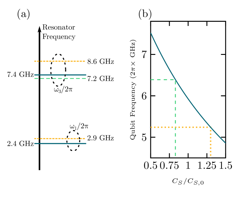
Figure 4: (a) The resonator frequency. The short-dashed (orange) lines indicate the eigenfrequencies ($\pi vn/l$) of the 1st and 3rd mode (marked by the circles) for an uncoupled transmission-line, while the values shown by solid blue lines are calculated using Eq. (II.1). The long-dashed green line is $3\omega_{1}$, with $\omega_{1}$ being the experimentally measured frequency of the 1st mode. (b) The qubit frequency calculated by diagonalizing Eq. (29) is shown as function of the shunt capacitance $C_{S}$ in units of the value $C_{S,0}$ estimated from the experimental parameters. The dashed green and orange lines show the measured qubit frequencies for the first and second qubits and the corresponding effective shunt capacitances.

The system studied in Rehák et al. (2014) is illustrated in the circuit diagram in Fig. 3 with 11 Josephson junctions placed in two loops. In each loop the three small junctions constitute a flux qubit with $C_{J}=3$ fF and $E_{J}=2\pi\times 60$ GHz and $\alpha=0.5$. The two lower resonator coupling junctions, 5 and 10, have areas 10 times larger than the $\alpha$ junction and the side junction capacitances, 1, 6 and 11, are yet again 10 times larger than the ones of the resonator coupling junctions. The qubits are cross coupled by the junction, 6, using a twist technique introduced in Grajcar et al. (2005) which ensure that $H_{c}\sim-G_{12}$.

We can calculate the resonator frequency using Eq. (II.1), presented in Fig. 4 (a), and the two qubit frequencies, shown in Fig. 4 (b). Treating the resonator length, $l$, as an adjustable parameter we match the fundamental mode to the experimental value of $\omega_{1}=2\pi\times 2.4$ GHz, and our theory then yields the eigenfrequency of the third mode, $\omega_{3}=2\pi\times 7.4\text{ GHz}\neq 3\omega_{1}$ which exactly match the experimentally measured value and is a first indication that our theory describes the experiment well.

The qubit frequency can be calculated by diagonalization of the Hamiltonian Eq. (29). If we calculate the shunt capacitance, $C_{S,0}$, from the serial line of capacitances of the three large junctions 1,5 and 6 (equivalent to 6, 10 and 11) we obtain a qubit frequency of $\omega_{10}=2\pi\times 5.9$ GHz, different from the measured values $\omega_{10}^{(1)}=2\pi\times 6.39$ GHz and $\omega_{10}^{(2)}=2\pi\times 5.28$ Neilinger et al. (2015). By allowing adjustment of the shunt capacitances, $C_{S}$, for both qubits we can, however, reproduce the correct qubit frequencies, see Fig. 4 (b).

After applying the parameter adjustments to match the frequency of each component, we can proceed and determine the non-linear properties of the system. From Eq. (26) we can thus directly calculate the Kerr constant for the third mode, which was probed in the experiment. We find a value of $K_{33}/\omega_{3}=-3\times 10^{-5}$, which is much smaller than the measured result and of the opposite sign. We know, however, that this expression does not properly take into account the Rabi splitting of the eigenmodes by the coupling to the qubit degrees of freedom. To evaluate the effects of the non-linear terms we must diagonalize the Hamiltonian,

$$H_{3} =\hbar\omega_{3}a^{\dagger}a+\frac{\hbar K_{33}}{2}a^{\dagger}aa^{\dagger}a+\frac{\hbar\omega_{10}^{(1)}}{2}\sigma_{z}^{(1)}+\frac{\hbar\omega_{10}^{(2)}}{2}\sigma_{z}^{(2)}$$

$$\quad+\hbar g_{3}^{(1)}\sigma_{x}^{(1)}(a^{\dagger}+a)+\hbar g_{3}^{(2)}\sigma_{x}^{(2)}(a^{\dagger}+a)$$

$$\quad-G_{12}\,\sigma_{x}^{(1)}\sigma_{x}^{(2)},$$ (36)

where $\sigma_{x}^{(i)}=(\ket{0^{(i)}}\bra{1^{(i)}}+\ket{1^{(i)}}\bra{0^{(i)}})$, and only then extract the effective Kerr constant, $\tilde{K}_{33}$.

We calculate the coupling strength $g_{3}^{(i)}$ using Eq. (32) where the flux differences $\delta u_{3}^{(1)}$ and $\delta u_{3}^{(2)}$ come from $\phi_{5}-\phi_{1}$ and $\phi_{4}-\phi_{8}$ of Fig. 3, respectively. The qubit-qubit coupling, $G_{12}$, is derived from the experimental design parameters and is negative due to the twisted coupling between $\phi_{5}$ and $\phi_{4}$. With these values and a numerical diagonalization of Eq. (IV), we obtain $\tilde{K}_{33}/\omega_{3}=2.1\times 10^{-3}$, which is, indeed, close to the experimentally obtained value. In comparison, for a single flux qubit (assuming $g_{3}^{(2)}=G_{12}=0$) we find $\tilde{K}_{33}^{(1)}/\omega_{3}=3.28\times 10^{-4}$.

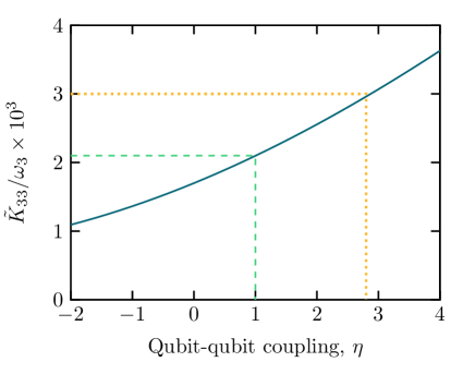
Figure 5: The effective Kerr constant $\tilde{K}_{33}^{(1)}/\omega_{3}$ as a function of the relative qubit-qubit coupling is shown as the solid blue line. The dashed green line marks the value obtained by directly using the experimental design parameters, while the orange dotted line marks the experimentally measure Kerr constant.

As we are expecting to underestimate the value of the qubit-qubit coupling, $G_{12}$, we have investigated the role of its value in the determination of $\tilde{K}_{33}^{(1)}/\omega_{3}$, by scaling it with a constant factor $G_{12}\rightarrow\eta\,G_{12}$ without changing the other parameters of the problem. Fig. 5 shows how the resulting effective Kerr coefficient depends on $\eta$. We observe that an increase in the qubit-qubit coupling leads to an increased Kerr constant but also that, even if the qubits do not interact directly, we still obtain a sizeable Kerr constant.

As also demonstrated in Rehák et al. (2014), the external flux can be tuned in-situ and, thus, yielding an effective tunable Kerr constant of the combined system. Most significantly, the external flux can be put at $\Phi_{x}=0$, where the qubit mode is negligible and, thus, the non-linearity is accurately predicted by Eq. (26). Thus we can both tune the sign and magnitude of the non-linearity.

V Conclusion and outlook

In this work we have presented a general framework to obtain an effective quantum description of a discrete circuit embedded in a transmission-line. Our approach treats the coupled systems by separately driving the circuit input and output nodes with current variables, which in turn, are forced to match the wave equation and boundary conditions for the transmission-line. This approach extends the successful Lagrangian formalism for quantization of circuit systems, which has been vastly successful in the field of circuit QED.

We illustrated the use of our method by an application to flux qubits, which allowed us to establish a full quantum model for a recent experiment performed by M. Rahák et.al. Rehák et al. (2014). By numerical diagonalization of the few mode quantum Hamiltonian, we were able to calculate the effective Kerr coefficient of the transmission-line in good agreement with the experimentally obtained value.

Our method may be directly applicable to any design using inductors, capacitors and Josephson junction embedded in a transmission-line resonator, and we expect that generalization is also possible to travelling wave systems, where it may be used to to describe the recently developed Josephson travelling wave parametric amplifiers Macklin et al. (2015); White et al. (2015); Grimsmo et al. (2016).

References

- Wallraff et al. (2004) Andreas Wallraff, David I Schuster, Alexandre Blais, L Frunzio, R-S Huang, J Majer, S Kumar, Steven M Girvin, and Robert J Schoelkopf, “Strong coupling of a single photon to a superconducting qubit using circuit quantum electrodynamics,” Nature 431, 162–167 (2004).
- Blais et al. (2004) Alexandre Blais, Ren-Shou Huang, Andreas Wallraff, S. M. Girvin, and R. J. Schoelkopf, “Cavity quantum electrodynamics for superconducting electrical circuits: An architecture for quantum computation,” Phys. Rev. A 69, 062320 (2004).
- Abdumalikov Jr et al. (2008) Abdufarrukh A Abdumalikov Jr, Oleg Astafiev, Yasunobu Nakamura, Yuri A Pashkin, and JawShen Tsai, “Vacuum rabi splitting due to strong coupling of a flux qubit and a coplanar-waveguide resonator,” Physical review b 78, 180502 (2008).
- Castellanos-Beltran et al. (2008) MA Castellanos-Beltran, KD Irwin, GC Hilton, LR Vale, and KW Lehnert, “Amplification and squeezing of quantum noise with a tunable josephson metamaterial,” Nature Physics 4, 929–931 (2008).
- Hatridge et al. (2011) M. Hatridge, R. Vijay, D. H. Slichter, John Clarke, and I. Siddiqi, “Dispersive magnetometry with a quantum limited squid parametric amplifier,” Phys. Rev. B 83, 134501 (2011).
- Rehák et al. (2014) M Rehák, P Neilinger, M Grajcar, G Oelsner, U Hübner, E Il’ichev, and H-G Meyer, “Parametric amplification by coupled flux qubits,” Applied Physics Letters 104, 162604 (2014).
- Astafiev et al. (2007) O Astafiev, K Inomata, AO Niskanen, T Yamamoto, Yu A Pashkin, Y Nakamura, and JS Tsai, “Single artificial-atom lasing,” Nature 449, 588–590 (2007).
- Neilinger et al. (2015) P. Neilinger, M. Rehák, M. Grajcar, G. Oelsner, U. Hübner, and E. Il’ichev, “Two-photon lasing by a superconducting qubit,” Phys. Rev. B 91, 104516 (2015).
- Van Loo et al. (2013) Arjan F Van Loo, Arkady Fedorov, Kevin Lalumière, Barry C Sanders, Alexandre Blais, and Andreas Wallraff, “Photon-mediated interactions between distant artificial atoms,” Science 342, 1494–1496 (2013).
- Pozar (2009) David M Pozar, Microwave engineering (John Wiley & Sons, 2009).
- Nigg et al. (2012) Simon E. Nigg, Hanhee Paik, Brian Vlastakis, Gerhard Kirchmair, S. Shankar, Luigi Frunzio, M. H. Devoret, R. J. Schoelkopf, and S. M. Girvin, “Black-box superconducting circuit quantization,” Phys. Rev. Lett. 108, 240502 (2012).
- Bourassa et al. (2012) J. Bourassa, F. Beaudoin, Jay M. Gambetta, and A. Blais, “Josephson-junction-embedded transmission-line resonators: From kerr medium to in-line transmon,” Phys. Rev. A 86, 013814 (2012).
- Leib et al. (2012) Martin Leib, Frank Deppe, Achim Marx, Rudolf Gross, and MJ Hartmann, “Networks of nonlinear superconducting transmission line resonators,” New Journal of Physics 14, 075024 (2012).
- Eichler and Wallraff (2014) Christopher Eichler and Andreas Wallraff, “Controlling the dynamic range of a josephson parametric amplifier,” EPJ Quantum Technology 1, 1–19 (2014).
- Nakamura et al. (1999) Yu Nakamura, Yu A Pashkin, and JS Tsai, “Coherent control of macroscopic quantum states in a single-cooper-pair box,” Nature 398, 786–788 (1999).
- Koch et al. (2007) Jens Koch, Terri M. Yu, Jay Gambetta, A. A. Houck, D. I. Schuster, J. Majer, Alexandre Blais, M. H. Devoret, S. M. Girvin, and R. J. Schoelkopf, “Charge-insensitive qubit design derived from the cooper pair box,” Phys. Rev. A 76, 042319 (2007).
- Mooij et al. (1999) JE Mooij, TP Orlando, L Levitov, Lin Tian, Caspar H Van der Wal, and Seth Lloyd, “Josephson persistent-current qubit,” Science 285, 1036–1039 (1999).
- Yan et al. (2015) F Yan, S Gustavsson, A Kamal, J Birenbaum, AP Sears, D Hover, TJ Gudmundsen, JL Yoder, TP Orlando, John Clarke, et al., “The flux qubit revisited,” arXiv preprint arXiv:1508.06299 (2015).
- Devoret (1995) Michel H Devoret, “Quantum fluctuations in electrical circuits,” (Les Houches, Session LXIII, 1995).
- Yurke and Denker (1984) Bernard Yurke and John S. Denker, “Quantum network theory,” Phys. Rev. A 29, 1419–1437 (1984).
- Weißl et al. (2015) T. Weißl, B. Küng, E. Dumur, A. K. Feofanov, I. Matei, C. Naud, O. Buisson, F. W. J. Hekking, and W. Guichard, “Kerr coefficients of plasma resonances in josephson junction chains,” Phys. Rev. B 92, 104508 (2015).
- Leib and Hartmann (2014) Martin Leib and Michael J. Hartmann, “Synchronized switching in a josephson junction crystal,” Phys. Rev. Lett. 112, 223603 (2014).
- Eichler et al. (2014) C. Eichler, Y. Salathe, J. Mlynek, S. Schmidt, and A. Wallraff, “Quantum-limited amplification and entanglement in coupled nonlinear resonators,” Phys. Rev. Lett. 113, 110502 (2014).
- Andersen and Mølmer (2015) Christian Kraglund Andersen and Klaus Mølmer, “Multifrequency modes in superconducting resonators: Bridging frequency gaps in off-resonant couplings,” Phys. Rev. A 91, 023828 (2015).
- Taylor (2005) John R. Taylor, Classical Mechanics (University Science Books, 2005).
- Bourassa et al. (2009) J. Bourassa, J. M. Gambetta, A. A. Abdumalikov, O. Astafiev, Y. Nakamura, and A. Blais, “Ultrastrong coupling regime of cavity qed with phase-biased flux qubits,” Phys. Rev. A 80, 032109 (2009).
- Orlando et al. (1999) TP Orlando, JE Mooij, Lin Tian, Caspar H van der Wal, LS Levitov, Seth Lloyd, and JJ Mazo, “Superconducting persistent-current qubit,” Physical Review B 60, 15398 (1999).
- Grajcar et al. (2005) M. Grajcar, A. Izmalkov, S. H. W. van der Ploeg, S. Linzen, E. Il’ichev, Th. Wagner, U. Hübner, H.-G. Meyer, Alec Maassen van den Brink, S. Uchaikin, and A. M. Zagoskin, “Direct josephson coupling between superconducting flux qubits,” Phys. Rev. B 72, 020503 (2005).
- Grajcar et al. (2006) M. Grajcar, A. Izmalkov, S. H. W. van der Ploeg, S. Linzen, T. Plecenik, Th. Wagner, U. Hübner, E. Il’ichev, H.-G. Meyer, A. Yu. Smirnov, Peter J. Love, Alec Maassen van den Brink, M. H. S. Amin, S. Uchaikin, and A. M. Zagoskin, “Four-qubit device with mixed couplings,” Phys. Rev. Lett. 96, 047006 (2006).
- Macklin et al. (2015) C Macklin, K O’Brien, D Hover, ME Schwartz, V Bolkhovsky, X Zhang, WD Oliver, and I Siddiqi, “A near–quantum-limited josephson traveling-wave parametric amplifier,” Science 350, 307–310 (2015).
- White et al. (2015) TC White, JY Mutus, I-C Hoi, R Barends, B Campbell, Yu Chen, Z Chen, B Chiaro, A Dunsworth, E Jeffrey, et al., “Traveling wave parametric amplifier with josephson junctions using minimal resonator phase matching,” Applied Physics Letters 106, 242601 (2015).
- Grimsmo et al. (2016) Arne Grimsmo, Aashish Clerk, and Alexandre Blais, “Engineering non-classical light with non-linear microwaveguides,” Bulletin of the American Physical Society (2016).