Geodesic ball packings generated by regular prism tilings in $\mathbf{Nil}$ geometry

Abstract

In this paper we study the regular prism tilings and construct ball packings by geodesic balls related to the above tilings in the projective model of $\mathbf{Nil}$ geometry. Packings are generated by action of the discrete prism groups $\mathbf{pq2_{1}}$. We prove that these groups are realized by prism tilings in $\mathbf{Nil}$ space if $(p,q)=(3,6),(4,4),(6,3)$ and determine packing density formulae for geodesic ball packings generated by the above prism groups. Moreover, studying these formulae we determine the conjectured maximal dense packing arrangements and their densities and visualize them in the projective model of $\mathbf{Nil}$ geometry. We get a dense (conjectured locally densest) geodesic ball arrangement related to the parameters $(p,q)=(6,3)$ where the kissing number of the packing is $14$, similarly to the densest lattice-like $\mathbf{Nil}$ geodesic ball arrangement investigated by the second author in [22].

1 Introduction and previous results

In mathematics sphere packing problems concern the arrangements of non-overlapping equal spheres which fill a space. Usually the space involved is the three-dimensional Euclidean space where the famous Kepler conjecture was proved by T. C. Hales and S. P. Ferguson in [5].

However, ball (sphere) packing problems can be generalized to the other $3$-dimensional Thurston geometries.

In an $n$-dimensional space of constant curvature $\mathbf{E}^{n}$, $\mathbf{H}^{n}$, $\mathbf{S}^{n}$ $(n\geq 2)$ let $d_{n}(r)$ be the density of $n+1$ spheres of radius $r$ mutually touching one another with respect to the simplex spanned by the centres of the spheres. L. Fejes Tóth and H. S. M. Coxeter conjectured that in an $n$-dimensional space of constant curvature the density of packing spheres of radius $r$ can not exceed $d_{n}(r)$. This conjecture has been proved by C. Roger in the Euclidean space. The 2-dimensional case has been solved by L. Fejes Tóth. In an $3$-dimensional space of constant curvature the problem has been investigated by Böröczky and Florian in [2] and it has been studied by K. Böröczky in [3] for $n$-dimensional space of constant curvature $(n\geq 4)$.

In [6], [7], [24] and [27] we have studied some new aspects of the horoball and hyperball packings in $\mathbf{H}^{n}$ and we have observed that the ball, horoball and hyperball packing problems are not settled yet in the $n$-dimensional $(n\geq 3)$ hyperbolic space.

In [28] we generalized the above problem of finding the densest geodesic and translation ball (or sphere) packing to the other $3$-dimensional homogeneous geometries (Thurston geometries)

$$\widetilde{\mathbf{S}\mathbf{L}_{2}\mathbf{R}},\leavevmode\nobreak\ \mathbf{Nil},\leavevmode\nobreak\ \mathbf{S}^{2}\!\times\!\mathbf{R},\leavevmode\nobreak\ \mathbf{H}^{2}\!\times\!\mathbf{R},\leavevmode\nobreak\ \mathbf{Sol},$$

and in the papers [21], [22], [23], [25], [28] we investigated several interesting ball packing and covering problems in the above geometries. We described in $\mathbf{S}^{2}\!\times\!\mathbf{R}$ geometry (see [28]) a candidate of the densest geodesic and translation ball arrangement whose density is $\approx 0.8750$.

In this paper we consider the $\mathbf{Nil}$ geometry that can be derived from W. Heisenberg’s famous real matrix group. This group provides a non-commutative translation group of an affine 3-space. E. Molnár proved in [10], that the homogeneous 3-spaces have a unified interpretation in the projective 3-sphere $\mathcal{PS}^{3}$. In this work we will use this projective model of the $\mathbf{Nil}$ geometry.

In [22] we investigated the geodesic balls of the $\mathbf{Nil}$ space and computed their volume, introduced the notion of the $\mathbf{Nil}$ lattice, $\mathbf{Nil}$ parallelepiped and the density of the lattice-like ball packing. Moreover, we determined the densest lattice-like geodesic ball packing. The density of this densest packing is $\approx 0.7809$, may be surprising enough in comparison with the Euclidean result $\frac{\pi}{\sqrt{18}}\approx 0.74048$. The kissing number of the balls in this packing is $14$.

In [25] we considered the analogue question for translation balls. The notions of translation curve and translation ball were introduced by initiative of E. Molnár (see [14], [21]). We have studied the translation balls of $\mathbf{Nil}$ space and computed their volume. Moreover, we have proved that the density of the optimal lattice-like translation ball packing for every natural lattice parameter $1\leq k\in\mathbf{N}$ is in interval $(0.7808,0.7889)$ and if $r\in(0,r_{d}]\ (r_{d}\approx 0.7456)$ then the optimal density is $\delta^{opt}\approx 0.7808$. Meanwhile we can apply a nice general estimate of L. Fejes Tóth [4] in our proof. The kissing number of the lattice-like ball packings is less than or equal to 14 and the optimal ball packing is realizable in case of equality. We formulated a conjecture for $\delta^{opt}$, where the density of the conjectural densest packing is $\delta^{opt}\approx 0.7808$ for lattice parameter $k=1$, larger than the Euclidean one ($\frac{\pi}{\sqrt{18}}\approx 0.7405$), but less than the density of the densest lattice-like geodesic ball packing in $\mathbf{Nil}$ space known till now [22]. The kissing number of the translation balls in that packing is 14 as well.

In [28] we studied one type of lattice coverings in the $\mathbf{Nil}$ space. We introduced the notion of the density of considered coverings and gave upper and lower estimation to the density of the lowest lattice-like geodesic ball covering. Moreover we formulate a conjecture for the ball arrangement of the least dense lattice-like geodesic ball covering and give its covering density $\Delta\approx 1.4290$.

In papers [25],[14] there are further results related to discrete problems of $\mathbf{Nil}$ geometry.

In this paper we study the regular prism tilings and construct ball packings by geodesic balls related to the prism tilings in the projective model of $\mathbf{Nil}$ geometry where the packings are generated by action of the discrete prism groups $\mathbf{pq2_{1}}$. We obtain density formulae for calculations for geodesic ball packings. Analyzing these density functions we obtain a conjecture for optimal geodesic ball packing configurations and determine their densities related to the above prismatic tessellations.

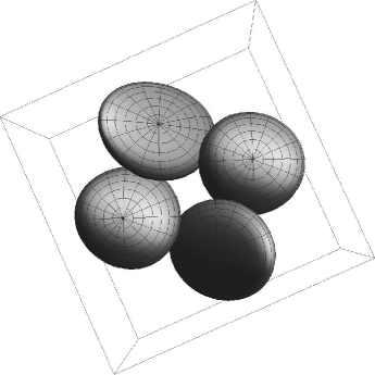
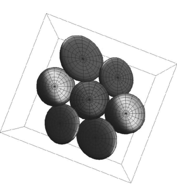
Figure 3: Some balls of the optimal ball arrangements for the square and hexagonal tilings shown from the direction of the $z$-axis.

The results are summarized in Theorems 3.4, 4.3 and Conjecture 4.4, and the optimal ball configurations are visualized in our model with Figures 2, 3.

2 Basic notions of the $\mathbf{Nil}$ geometry

In this Section we summarize the significant notions and denotations of the $\mathbf{Nil}$ geometry (see [10], [22]).

The $\mathbf{Nil}$ geometry is a homogeneous 3-space derived from the famous real matrix group $\mathbf{L(R)}$ discovered by W. Heisenberg. The Lie Theory with the method of the projective geometry makes possible to investigate and to describe this topic.

The left (row-column) multiplication of Heisenberg matrices

$$\begin{gathered}\begin{pmatrix}1&x&z\\ 0&1&y\\ 0&0&1\\ \end{pmatrix}\begin{pmatrix}1&a&c\\ 0&1&b\\ 0&0&1\\ \end{pmatrix}=\begin{pmatrix}1&a+x&c+xb+z\\ 0&1&b+y\\ 0&0&1\\ \end{pmatrix}\end{gathered}$$ (2.1)

defines ”translations” $\mathbf{L}(\mathbf{R})=\{(x,y,z):x,\leavevmode\nobreak\ y,\leavevmode\nobreak\ z\in\mathbf{R}\}$ on the points of the space $\mathbf{Nil}=\{(a,b,c):a,\leavevmode\nobreak\ b,\leavevmode\nobreak\ c\in\mathbf{R}\}$. These translations are not commutative in general. The matrices $\mathbf{K}(z)\vartriangleleft\mathbf{L}$ of the form

$$\begin{gathered}\mathbf{K}(z)\ni\begin{pmatrix}1&0&z\\ 0&1&0\\ 0&0&1\\ \end{pmatrix}\mapsto(0,0,z)\end{gathered}$$ (2.2)

constitute the one parametric centre, i.e. each of its elements commutes with all elements of $\mathbf{L}$. The elements of $\mathbf{K}$ are called fibre translations. $\mathbf{Nil}$ geometry of the Heisenberg group can be projectively (affinely) interpreted by the ”right translations” on points as the matrix formula

$$\begin{gathered}(1;a,b,c)\to(1;a,b,c)\begin{pmatrix}1&x&y&z\\ 0&1&0&0\\ 0&0&1&x\\ 0&0&0&1\\ \end{pmatrix}=(1;x+a,y+b,z+bx+c)\end{gathered}$$ (2.3)

shows, according to (1.1). Here we consider $\mathbf{L}$ as projective collineation group with right actions in homogeneous coordinates. We will use the Cartesian homogeneous coordinate simplex $E_{0}(\mathbf{e}_{0})$,$E_{1}^{\infty}(\mathbf{e}_{1})$,$E_{2}^{\infty}(\mathbf{e}_{2})$, $E_{3}^{\infty}(\mathbf{e}_{3}),\ (\{\mathbf{e}_{i}\}\subset\mathbf{V}^{4}$  with the unit point $E(\mathbf{e}=\mathbf{e}_{0}+\mathbf{e}_{1}+\mathbf{e}_{2}+\mathbf{e}_{3}))$ which is distinguished by an origin $E_{0}$ and by the ideal points of coordinate axes, respectively. Moreover, $\mathbf{y}=c\mathbf{x}$ with $0<c\in\mathbb{R}$ (or $c\in\mathbb{R}\setminus\{0\})$ defines a point $(\mathbf{x})=(\mathbf{y})$ of the projective 3-sphere $\mathcal{P}\mathcal{S}^{3}$ (or that of the projective space $\mathcal{P}^{3}$ where opposite rays $(\mathbf{x})$ and $(-\mathbf{x})$ are identified). The dual system $\{(\boldsymbol{e}^{i})\},\ (\{\mathbf{e}^{i}\}\subset\boldsymbol{V}_{4})$ describes the simplex planes, especially the plane at infinity $(\boldsymbol{e}^{0})=E_{1}^{\infty}E_{2}^{\infty}E_{3}^{\infty}$, and generally, $\boldsymbol{v}=\boldsymbol{u}\frac{1}{c}$ defines a plane $(\boldsymbol{u})=(\boldsymbol{v})$ of $\mathcal{P}\mathcal{S}^{3}$ (or that of $\mathcal{P}^{3}$). Thus $0=\mathbf{x}\boldsymbol{u}=\mathbf{y}\boldsymbol{v}$ defines the incidence of point $(\mathbf{x})=(\mathbf{y})$ and plane $(\boldsymbol{u})=(\boldsymbol{v})$, as $(\mathbf{x})\text{I}(\boldsymbol{u})$ also denotes it. Thus Nil can be visualized in the affine 3-space $\mathbf{A}^{3}$ (so in $\mathbf{E}^{3}$) as well.

The translation group $\mathbf{L}$ defined by formula (2.3) can be extended to a larger group $\mathbf{G}$ of collineations, preserving the fibering, that will be equivalent to the (orientation preserving) isometry group of $\mathbf{Nil}$. In [11] E. Molnár has shown that a rotation trough angle $\omega$ about the $z$-axis at the origin, as isometry of $\mathbf{Nil}$, keeping invariant the Riemann metric everywhere, will be a quadratic mapping in $x,y$ to $z$-image $\overline{z}$ as follows:

$$\begin{gathered}\mathbf{r}(O,\omega):(1;x,y,z)\to(1;\overline{x},\overline{y},\overline{z});\\ \overline{x}=x\cos{\omega}-y\sin{\omega},\ \ \overline{y}=x\sin{\omega}+y\cos{\omega},\\ \overline{z}=z-\frac{1}{2}xy+\frac{1}{4}(x^{2}-y^{2})\sin{2\omega}+\frac{1}{2}xy\cos{2\omega}.\end{gathered}$$ (2.4)

This rotation formula, however, is conjugate by the quadratic mapping $\mathcal{M}$

$$\begin{gathered}x\to x^{\prime}=x,\ \ y\to y^{\prime}=y,\ \ z\to z^{\prime}=z-\frac{1}{2}xy\ \ \text{to}\\ (1;x^{\prime},y^{\prime},z^{\prime})\to(1;x^{\prime},y^{\prime},z^{\prime})\begin{pmatrix}1&0&0&0\\ 0&\cos{\omega}&\sin{\omega}&0\\ 0&-\sin{\omega}&\cos{\omega}&0\\ 0&0&0&1\\ \end{pmatrix}=(1;x",y",z"),\\ \text{with}\ \ x"\to\overline{x}=x",\ \ y"\to\overline{y}=y",\ \ z"\to\overline{z}=z"+\frac{1}{2}x"y",\end{gathered}$$ (2.5)

i.e. to the linear rotation formula. This quadratic conjugacy modifies the $\mathbf{Nil}$ translations in (2.3), as well. We shall use the following important classification theorem.

Theorem 2.1 (E. Molnár [11])

1. Any group of $\mathbf{Nil}$ isometries, containing a 3-dimensional translation lattice, is conjugate by the quadratic mapping in (2.5) to an affine group of the affine (or Euclidean) space $\mathbf{A}^{3}=\mathbf{E}^{3}$ whose projection onto the (x,y) plane is an isometry group of $\mathbf{E}^{2}$. Such an affine group preserves a plane $\to$ point polarity of signature $(0,0,\pm 0,+)$.

2. Of course, the involutive line reflection about the $y$ axis

   $$\begin{gathered}(1;x,y,z)\to(1;-x,y,-z),\end{gathered}$$

   preserving the Riemann metric, and its conjugates by the above isometries in 1 (those of the identity component) are also $\mathbf{Nil}$-isometries. There does not exist orientation reversing $\mathbf{Nil}$-isometry.

Remark 2.2

We obtain from the above described projective model a new model of $\mathbf{Nil}$ geometry derived by the quadratic mapping $\mathcal{M}$. This is the linearized model of $\mathbf{Nil}$ space (see [1]).

2.1 Geodesic curves and spheres

The geodesic curves of the $\mathbf{Nil}$ geometry are generally defined as having locally minimal arc length between their any two (near enough) points. The equation systems of the parametrized geodesic curves $g(x(t),y(t),z(t))$ in our model can be determined by the general theory of Riemann geometry. We can assume, that the starting point of a geodesic curve is the origin because we can transform a curve into an arbitrary starting point by translation (2.1);

$$\begin{gathered}x(0)=y(0)=z(0)=0;\ \ \dot{x}(0)=c\cos{\alpha},\ \dot{y}(0)=c\sin{\alpha},\\ \dot{z}(0)=w;\ -\pi\leq\alpha\leq\pi.\end{gathered}$$

The arc length parameter $s$ is introduced by

$$s=\sqrt{c^{2}+w^{2}}\cdot t,\ \text{where}\ w=\sin{\theta},\ c=\cos{\theta},\ -\frac{\pi}{2}\leq\theta\leq\frac{\pi}{2},$$

i.e. unit velocity can be assumed.

Remark 2.3

Thus we have harmonized the scales along the coordinate axes.

The equation systems of a helix-like geodesic curves $g(x(t),y(t),z(t))$ if $0<|w|<1$:

$$\begin{gathered}x(t)=\frac{2c}{w}\sin{\frac{wt}{2}}\cos\Big{(}\frac{wt}{2}+\alpha\Big{)},\ \ y(t)=\frac{2c}{w}\sin{\frac{wt}{2}}\sin\Big{(}\frac{wt}{2}+\alpha\Big{)},\\ z(t)=wt\cdot\Big{\{}1+\frac{c^{2}}{2w^{2}}\Big{[}\Big{(}1-\frac{\sin(2wt+2\alpha)-\sin{2\alpha}}{2wt}\Big{)}+\\ +\Big{(}1-\frac{\sin(2wt)}{wt}\Big{)}-\Big{(}1-\frac{\sin(wt+2\alpha)-\sin{2\alpha}}{2wt}\Big{)}\Big{]}\Big{\}}=\\ =wt\cdot\Big{\{}1+\frac{c^{2}}{2w^{2}}\Big{[}\Big{(}1-\frac{\sin(wt)}{wt}\Big{)}+\Big{(}\frac{1-\cos(2wt)}{wt}\Big{)}\sin(wt+2\alpha)\Big{]}\Big{\}}.\end{gathered}$$ (2.6)

In the cases $w=0$ the geodesic curve is the following:

$$x(t)=c\cdot t\cos{\alpha},\ \ y(t)=c\cdot t\sin{\alpha},\ \ z(t)=\frac{1}{2}\leavevmode\nobreak\ c^{2}\cdot t^{2}\cos{\alpha}\sin{\alpha}.$$ (2.7)

The cases $|w|=1$ are trivial: $(x,y)=(0,0),\ z=w\cdot t$.

Definition 2.4

The distance $d(P_{1},P_{2})$ between the points $P_{1}$ and $P_{2}$ is defined by the arc length of geodesic curve from $P_{1}$ to $P_{2}$.

In our work [22] we introduced the following definitions:

Definition 2.5

The geodesic sphere of radius $R$ with centre at the point $P_{1}$ is defined as the set of all points $P_{2}$ in the space with the condition $d(P_{1},P_{2})=R$. Moreover, we require that the geodesic sphere is a simply connected surface without self-intersection in the $\mathbf{Nil}$ space.

Remark 2.6

We shall see that this last condition depends on radius $R$.

Definition 2.7

The body of the geodesic sphere of centre $P_{1}$ and of radius $R$ in the $\mathbf{Nil}$ space is called geodesic ball, denoted by $B_{P_{1}}(R)$, i.e. $Q\in B_{P_{1}}(R)$ iff $0\leq d(P_{1},Q)\leq R$.

Remark 2.8

Henceforth, typically we choose the origin as centre of the sphere and its ball, by the homogeneity of $\mathbf{Nil}$.

We have denoted by $B(S)$ the body of the $\mathbf{Nil}$ sphere $S$, furthermore we have denoted their volumes by $Vol(B(S))$.

In [22] we have proved the the following theorem:

Theorem 2.9

The geodesic sphere and ball of radius $R$ exists in the $\mathbf{Nil}$ space if and only if $R\in[0,2\pi].$

We obtain the volume of the geodesic ball of radius $R$ by the following integral (see 2.8):

$$\begin{gathered}Vol(B(S))=2\pi\int_{0}^{\frac{\pi}{2}}X^{2}\leavevmode\nobreak\ \frac{\mathrm{d}\leavevmode\nobreak\ Z}{\mathrm{d}\leavevmode\nobreak\ \theta}\leavevmode\nobreak\ \mathrm{d}\leavevmode\nobreak\ {\theta}=\\ =2\pi\int_{0}^{\frac{\pi}{2}}\Big{(}\frac{2\cos{\theta}}{\sin{\theta}}\sin{\frac{(R\sin{\theta})}{2}}\Big{)}^{2}\cdot\Big{(}-\frac{1}{2}\frac{R\cos^{3}{\theta}}{\sin^{2}{\theta}}+\frac{\cos{\theta}\sin{(R\sin{\theta})}}{\sin{\theta}}+\\ +\frac{\cos^{3}{\theta}\sin{(R\sin{\theta})}}{\sin^{3}{\theta}}-\frac{1}{2}\frac{R\cos^{3}{\theta}\cos{(R\sin{\theta})}}{\sin^{2}{\theta}}\Big{)}{\mathrm{d}\leavevmode\nobreak\ \theta}.\end{gathered}$$ (2.8)

The parametric equation system of the geodesic sphere $S(R)$ in our model (see [22]):

$$\begin{gathered}x(R,\theta,\phi)=\frac{2c}{w}\sin{\frac{wR}{2}}\cdot\cos{\phi}=\frac{2\cos{\theta}}{\sin{\theta}}\sin{\frac{R\sin{\theta}}{2}}\cdot\cos{\phi},\\ y(R,\theta,\phi)=\frac{2c}{w}\sin{\frac{wR}{2}}\cdot\sin{\phi}=\frac{2\cos{\theta}}{\sin{\theta}}\sin{\frac{R\sin{\theta}}{2}}\cdot\sin{\phi},\\ z(R,\theta,\phi)=wR+\frac{c^{2}R}{2w}-\frac{c^{2}}{2w^{2}}\sin{wR}+\frac{1}{4}\Big{(}\frac{2c}{w}\sin{\frac{wR}{2}}\Big{)}^{2}\sin{2\phi}=\\ =R\sin{\theta}+\frac{R\cos^{2}{\theta}}{2\sin{\theta}}-\frac{\cos^{2}{\theta}}{2\sin^{2}{\theta}}\sin(R\sin{\theta})+\frac{1}{4}\Big{(}\frac{2\cos{\theta}}{\sin{\theta}}\sin{R\frac{\sin{\theta}}{2}}\Big{)}^{2}\sin{2\phi}\\ \end{gathered}$$

$$\begin{gathered}-\pi<\phi\leqq\pi,\ \ -\frac{\pi}{2}\leqq\theta\leqq\frac{\pi}{2}\ \text{and}\ \theta\neq 0.\\ \text{if}\ \theta=0\ \text{then}\ x(R,0,\phi)=R\cos{\phi},\ \ y(R,0,\phi)=R\sin{\phi},\\ \ z(R,0,\phi)=\frac{1}{2}\leavevmode\nobreak\ R^{2}\cos{\phi}\sin{\phi}.\end{gathered}$$ (2.9)

We have obtained by the derivatives of these parametrically represented functions (by intensive and careful computations with Maple through the second fundamental form) the following theorem (see [22]):

Theorem 2.10

The geodesic $\mathbf{Nil}$ ball $B(S(R))$ is convex in affine-Euclidean sense in our model if and only if $R\in[0,\frac{\pi}{2}]$.

3 $\mathbf{Nil}$ prisms and prism tilings

The prisms and prism-like tilings have been thoroughly investigated in $\mathbf{S}^{2}\!\times\!\mathbf{R},\mathbf{H}^{2}\!\times\!\mathbf{R}$ and $\widetilde{\mathbf{S}\mathbf{L}_{2}\mathbf{R}}$ spaces in papers [16], [19], [30]. Here we consider the analogous problem in $\mathbf{Nil}$ space. We will use the in 2. section described projective model of $\mathbf{Nil}$ geometry. In the following the plane of $x,\leavevmode\nobreak\ y$ axis are called base plane of the model and if we say plane then it is a plane in Euclidean sense.

Definition 3.1

Let $\mathcal{P}^{i}$ be an infinite solid bounded by planes, that are determined by fibre-lines passing through the points of a $p$-gon ($p\geq 3$, integer parameter) $\mathcal{P}^{b}$ lying in the base-plane. The images of $\mathcal{P}^{i}$ by $\mathbf{Nil}$ isometries are called infinite $p$-sided prisms.

The common part of $\mathcal{P}^{i}$ with the base plane is defined as the base figure $\mathcal{P}^{b}$ of the prism.

Let $\mathcal{F}$ be the $\mathcal{M}^{-1}$ image of the base plane in the $\mathbf{Nil}$-space (see Remark 2.2) and let $\tau$ be a fibre translation (2.2).

Definition 3.2

Let $\mathcal{P}^{i}$ be an infinite $p$-sided prism, that is trimmed by the surface $\mathcal{F}$ and its translated copy $\mathcal{F}^{\tau}$. The parts of $\mathcal{F}$ and $\mathcal{F}^{\tau}$ inside the infinite prism are called cover faces and are denoted by $C_{\mathcal{F}}$ and $C_{\mathcal{F}^{\tau}}$.

The $p$-sided bounded prism is the part of $\mathcal{P}^{i}$ between the cover faces $C_{\mathcal{F}}$ and $C_{\mathcal{F}^{\tau}}$.

Definition 3.3

A bounded or infinite $p$-sided prism is said to be regular if its side surfaces are congruent to each other under $\mathbf{Nil}$ rotations with angle $\frac{2\pi}{p}$ (see (2.4) and (2.5)) about the central fibre line of the prism.

3.1 Regular bounded prism tilings

In this section we will investigate the existence of regular bounded prism tilings $\mathcal{T}_{p}(q)$ of $\mathbf{Nil}$ space. In this case the prism tiles are regular bounded prisms having $p$-gonal base figures $(p\geq 3)$. The prism itself is a topological polyhedron with $2p$ vertices, and having at every vertex one $p$-gonal cover face and two quadrangle side faces (traced by fibre lines). We are looking such prism tilings of $\mathbf{Nil}$ space where at each side edge of the prism (which are fibre lines going through vertices of the base figure) meet $q$ prisms regularly, by $\mathbf{Nil}$ rotations with angle $\frac{2\pi}{q}$ ($q\geq 3$, integer parameter).

We shall see in Theorem 3.4 that the regular prism tiling $\mathcal{T}_{p}(q)$ exists for some parameters $(p,q)$. Let $\mathcal{P}_{p}(q)$ one of its tiles with with vertices $A_{1}A_{2}\dots A_{p}$ $B_{1}B_{2}\dots B_{p}$. We may assume that $A_{1}$ lies on the $x$-axis. It is clear that the side curves $c_{A_{i}A_{i+1}}$ $(i=1\dots p,\leavevmode\nobreak\ A_{p+1}\equiv A_{1})$ are derived from each other by $\frac{2\pi}{p}$ rotation about the $x$ axis. The corresponding vertices $B_{1}B_{2}\dots B_{p}$ are generated by a fibre translation $\tau$ with a positive real parameter. The cover faces $A_{1},\dots,A_{p}$, $B_{1},\dots,B_{p}$ and the side surfaces form a $p$-sided regular prism $\mathcal{P}_{p}(q)$ in $\mathbf{Nil}$. $\mathcal{T}_{p}(q)$ will be generated by its rotational isometry group $\Gamma_{p}(q)=\mathbf{pq2_{1}}$ $\subset Isom(\mathbf{Nil})$ (if these tiling there exist see Theorem 3.4) which is given by its fundamental domain $\mathcal{F}_{p}(q)=A_{1}A_{2}OA_{1}^{\mathbf{s}}A_{2}^{\mathbf{s}}O^{\mathbf{s}}$, $A_{1}^{\mathbf{s}}=B_{p}$. Here, $A_{2}^{\mathbf{s}}=B_{1}$, $O^{\mathbf{s}}=O^{\tau}$, and $\mathcal{F}_{p}(q)$ is a piece-wise linear topological polyhedron. The group presentation can be determined by a standard procedure [8], called Poincaré algorithm. The generators will pair the bent (piecewise linear) faces of $\mathcal{F}$:

$$\begin{gathered}\mathbf{a}\leavevmode\nobreak\ :\leavevmode\nobreak\ OA_{1}B_{p}O^{\mathbf{s}}(O)\rightarrow OA_{2}B_{1}O^{\mathbf{s}}(O),\\ \mathbf{b}\leavevmode\nobreak\ :\leavevmode\nobreak\ A_{1}A_{2}B_{1}(A_{1})\rightarrow A_{1}B_{p}B_{1}(A_{1}),\leavevmode\nobreak\ \mathbf{s}\leavevmode\nobreak\ :\leavevmode\nobreak\ OA_{1}A_{2}(O)\rightarrow O^{\mathbf{s}}B_{p}B_{1}(O^{\mathbf{s}})\end{gathered}$$

mapping $\mathcal{F}_{p}(q)$ onto its neighbours ${\mathcal{F}_{p}(q)}^{\mathbf{a}}$, ${\mathcal{F}_{p}(q)}^{\mathbf{b}}$, ${\mathcal{F}_{p}(q)}^{\mathbf{s}}$, respectively. E.g. for the face $a^{-1}$ a point $A$ (relative freely, e.g. in the segment $OB_{p}$) is taken. Then the union of triangles $AOO^{\mathbf{s}}$, $AO^{\mathbf{s}}B_{p}$, $AB_{p}A_{1}$, $OA_{1}O$ will be the face $a^{-1}$.

Then the $\mathbf{a}$-image $A^{\mathbf{a}}$ is taken in $OB_{1}$ for the face $a=A^{\mathbf{a}}OO^{\mathbf{s}}\cup A^{\mathbf{a}}O^{\mathbf{s}}B_{1}\cup A^{\mathbf{a}}B_{1}A_{2}\cup A^{\mathbf{a}}A_{2}O$, as usual. The relations are induced by the edge equivalence classes $\{OO^{\prime}\}$; $\{A_{1}B_{1}\}$; $\{OA_{1},$ $OA_{2},O^{\prime}B_{1},O^{\prime}B_{p}\}$; $\{A_{1}A_{2},A_{1}B_{p},A_{2}B_{1},B_{p}B_{1}\}$. So we get the group

$$\mathbf{pq2_{1}}=\{\mathbf{a},\mathbf{b}:\mathbf{a}^{p}=\mathbf{b}^{q}=\mathbf{a}\mathbf{b}\mathbf{a}\mathbf{b}\mathbf{a}^{-1}\mathbf{b}^{-1}\mathbf{a}^{-1}\mathbf{b}^{-1}=1\},$$ (3.1)

where $\mathbf{a}$ is a $p$ rotation about the fibre line through the origin (the $z$-axis), $\mathbf{b}$ is a $q$ rotation about a side fibre line of $\mathcal{P}_{p}(q)$ (through a vertex of its base figure). Notice, that $\mathbf{b}\mathbf{a}\mathbf{b}$ is a screw motion, and thus $\tau:=\mathbf{a}\mathbf{b}\mathbf{a}\mathbf{b}=\mathbf{b}\mathbf{a}\mathbf{b}\mathbf{a}$ is the fibre translation connecting the cover faces.

Our first question is the following: For which $3\leq p,q\in\mathbb{N}$ is $\Gamma_{p}(q)=\mathbf{pq2_{1}}\subset\mathit{Isom}(\mathbf{Nil})$?

The following Theorem answers it:

Theorem 3.4

In $\mathbf{Nil}$ there exist $3$ regular $p$-gonal non-face-to-face prism tilings $\mathcal{T}_{p}(q)$ with $\mathbf{Nil}$ isometry group $\Gamma_{p}(q)=\mathbf{pq2_{1}}$ for integer parameters $p,q\geq 3$:

the regular triangular prism tiling with $(p,q)=(3,6)$,

the regular square prism tiling with $(p,q)=(4,4)$,

the regular hexagonal prism tiling with $(p,q)=(6,3)$,

and each group $\Gamma_{p}(q)$ has a free parameter $x_{p}(q)\in\mathbb{R}^{+}$.

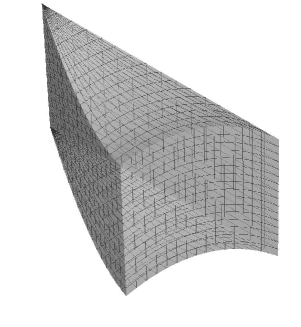
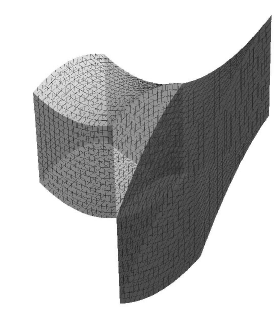
Figure 1: The regular triangular and rectangular prisms in $\mathbf{Nil}$-space, with parameters $x_{3}(6)=\frac{2}{\sqrt{3}}$ and $x_{4}(4)=\sqrt{2}$ respectively

Proof:

Let $A_{1}=(1;x_{p}(q),0,0)$ be a ”bottom” vertex of the regular bounded prism. Then the other vertices of the bottom cover face can be generated by the $\mathbf{Nil}$ rotation formula (see (2.4), (2.5)):

$$A_{2}=A_{1}^{\mathbf{a}}=\Big{(}1;x_{p}(q)\cos\Big{(}\frac{2\pi}{p}\Big{)},x_{p}(q)\sin\Big{(}\frac{2\pi}{p}\Big{)},\frac{1}{4}{x_{p}(q)}^{2}\sin\Big{(}\frac{4\pi}{p}\Big{)}\Big{)},$$

$$A_{3}=A_{2}^{\mathbf{a}}=A_{1}^{\mathbf{a}^{2}}=\Big{(}1;x_{p}(q)\cos\Big{(}\frac{4\pi}{p}\Big{)},x_{p}(q)\sin\Big{(}\frac{4\pi}{p}\Big{)},\frac{1}{4}x_{p}(q)^{2}\sin\Big{(}\frac{8\pi}{p}\Big{)}\Big{)},$$

$$\dots$$

$$A_{p}=A_{p-1}^{\mathbf{a}}=A_{p-1}^{\mathbf{a}^{p-1}}.$$

Then the condition for the existence of the tiling is the following:

$$A_{3}=A_{2}^{\mathbf{a}}\equiv A_{1}^{\mathbf{b}^{-1}},$$ (3.2)

where $\mathbf{a}$ is a $p$ rotation about the fibre line through the origin and $\mathbf{b}$ is a $q$ rotation about the side fibre line of $\mathcal{P}_{p}(q)$ through the vertex $A_{2}$. $\equiv$ means that the corresponding points lie on the same fibre lines.

$$1=\cos^{2}\Big{(}\frac{\pi}{p}\Big{)}+\cos^{2}\Big{(}\frac{\pi}{q}\Big{)},$$

where $p$ and $q$ are positive integers. This equation only has the following integer solutions:

$$(p,q)=(4,4),(3,6)\text{ or }(6,3).$$

We obtain from the above computations, that the existence of the above regular prism tilings is independent from the parameter $x_{p}(q)\in\mathbb{R}^{+}$, so we have proven the Theorem.   $\square$

Remembering that $\tau=\mathbf{a}\mathbf{b}\mathbf{a}\mathbf{b}$ is the ”vertical” translation of the group, we can also compute the height of the regular bounded prism corresponding to the group tiling, since: $O^{\mathbf{a}\mathbf{b}\mathbf{a}\mathbf{b}}=O^{\tau},$ where $O$ is the origin. Using this, we can also give a metric representation of the group, allowing the visualization of the corresponding prism and prism tiling (see Fig. 1. and Fig. 2.).

4 The optimal geodesic ball packings under group $\mathbf{pq2_{1}}$

The sphere packing problem deals with the arrangements of non-overlapping equal spheres, or balls, which fill the space. While the usual problem is in the $n$-dimensional Euclidean-space $(n\geq 2$), it can be generalized to the other $3$-dimensional Thurston spaces (see [29]). In this paper we investigate the optimal ball packings of $\mathbf{Nil}$ generated by the above described $\mathbf{pq2_{1}}$ group.

Let $\mathcal{T}_{p}(x_{p}(q),q)$ (where $(p,q)=(3,6),(4,4)$ or $(6,3)$ as stated above and $x_{p}(q)\in\mathbb{R}^{+}$) be a regular prism tiling, and let $\mathcal{P}_{p}(x_{p}(q),q)$ be one of its tiles that is centered at the origin, with a base face given by the vertices $A_{1},A_{2},\dots,A_{p}$. The corresponding vertices $B_{1},B_{2},\dots,B_{p}$ of the prism are generated by fibre translations $\tau=\mathbf{a}\mathbf{b}\mathbf{a}\mathbf{b}$.

We can assume by symmetry, that the optimal geodesic ball is centered at the origin. The volume of a geodesic ball with radius $R$ can be determined by the formula (2.8).

We study only one case of the multiply transitive geodesic ball packings where the fundamental domains of the $\mathbf{Nil}$ space groups $\mathbf{pq2_{1}}$ are not prisms. Let the fundamental domains be derived by the Dirichlet — Voronoi cells (D-V cells) where their centers are images of the origin. The volume of the $p$-times fundamental domain and of the D-V cell is the same, respectively, as in the prism case (for any above $(p,q,x_{p}(q))$ fixed). It is easy to see by the formulas (2.5), using the quadratic mapping $\mathcal{M}$, that the volume of the Dirichlet — Voronoi cell (or the coresponding prism) is

$$Vol(\mathcal{P}_{p}(x_{p}(q),q))=\frac{p}{2}{x_{p}^{2}(q)}\sin\Big{(}\frac{2\pi}{p}\Big{)}d(OO^{\tau}).$$ (4.1)

These locally densest geodesic ball packings can be determined for all possible fixed integer parameters $p,q,x_{p}(q)$. The optimal radius $R_{opt}(x_{p}(q))$ is

$$R_{opt}(x_{p}(q),p,q)=\min\Big{\{}d{(OA_{1})},\ \frac{d(OO^{\tau})}{2},\ \frac{d(O,O^{{\mathbf{a}}{\mathbf{b}}})}{2}\Big{\}},$$ (4.2)

where $d$ is the geodesic distance function of $\mathbf{Nil}$ geometry (see Definition 2.4).

Since the congruent images of $\mathcal{P}_{p}(x_{p}(q),q)$ under the discrete group $\mathbf{pq2_{1}}$ cover the $\mathbf{Nil}$ space, therefore for the density of the ball packing it is sufficient to relate the volume of the ball to the volume of the prism:

Definition 4.1

The maximal density $\delta_{p}(x_{p}(q),q)$ of the above multiply transitive ball packing for given parameters $(p,q,x_{p}(q))$ ($(p,q)=(3,6),(4,4),(6,3)$ and $x_{p}(q)\in\mathbb{R}^{+}$):

$$\delta_{p}(x_{p}(q),q)=\frac{Vol(B(R_{opt}))}{Vol(\mathcal{P}_{p}(x_{p}(q),q))}=\frac{Vol(B(R_{opt}))}{\frac{p}{2}{x_{p}^{2}(q)}\sin\Big{(}\frac{2\pi}{p}\Big{)}d(OO^{\tau})}.$$ (4.3)

For every $p,q,x_{p}(q)$ parameters the locally densest geodesic ball packing can be determined.

If we fixed the parameters $p$ and $q$ then the distance function $d(x_{p}(q))$ is a continuous fuction. Therefore it is easy prove the following Lemma:

Lemma 4.2

In $\mathbf{Nil}$-space for the rotation group $\Gamma_{p}(q)=\mathbf{pq2_{1}}$ there always exist $x_{p}(q)\in\mathbb{R}^{+}$ for given parameters $(p,q)=(4,4),(3,6),(6,3)$ where

$$d(O,O^{\mathbf{a}\mathbf{b}})=d(O,O^{\mathbf{a}\mathbf{b}\mathbf{a}\mathbf{b}})=d(O,O^{\tau}).$$ (4.4)

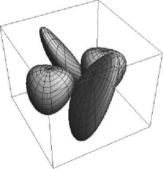
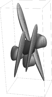
Figure 2: Some balls of the optimal ball arrangements for the square and hexagonal tilings with parameters $(p,q)=(4,4)$ and $(p,q)=(3,6)$.

The system of equations (4.4) in Lemma 4.2 can be solved by numerical methods and the corresponding ball arrangements are denoted by $\mathcal{B}_{p}(q)$. We obtain - using the formulas (4.1-3) - that in $\mathbf{Nil}$-space for the rotation group $\Gamma_{p}(q)=\mathbf{pq2_{1}}$ the metric data of the godesic ball arrangements $\mathcal{B}_{p}(q)$ are the following:

Theorem 4.3

If the system of equation (4.4) holds then the maximal radii and densities of the optimal ball packings are the following:

• If $(p,q)=(3,6)$, then $\delta_{p}(q)\approx 0.2593$, with $R_{opt}(p,q)\approx 0.7389$,

• If $(p,q)=(4,4)$, then $\delta_{p}(q)\approx 0.6512$, with $R_{opt}(p,q)\approx 1.2154$,

• If $(p,q)=(6,3)$, then $\delta_{p}(q)\approx 0.7272$, with $R_{opt}(p,q)\approx 1.9601$.

If we vary the parameter $x_{p}(q)$ in the above cases then the corresponding radius $R_{opt}(p,q)$ and the density $\delta_{p}(q)$ also change. The following table shows that probably the $\mathcal{B}_{p}(q)$ ball packings with maximal kissing numbers provide the optimal ball packing densities.

$(p,q)$	Radius	Prism volume	Density	Kissing number
(3,6)	0.5876	4.1446	0.2063	2
	0.6392	4.9032	0.2246	2
	0.6929	5.7616	0.2438	2
	0.7389	6.5517	0.2593	8
	0.7787	7.8111	0.2558	6
	0.8132	9.0201	0.2525	6
	0.8481	10.3641	0.2495	6
(4,4)	0.9927	7.8849	0.5283	2
	1.0644	9.0650	0.5678	2
	1.1386	10.3729	0.6090	2
	1.2154	11.8175	0.6512	10
	1.2594	13.4079	0.6404	8
	1.3036	15.1538	0.6295	8
	1.3480	17.0647	0.6194	8
(6,3)	1.6934	34.4141	0.6190	2
	1.7801	38.0287	0.6537	2
	1.8690	41.9209	0.6897	2
	1.9601	46.1044	0.7272	14
	2.0087	50.5935	0.7153	12
	2.0573	55.4028	0.7038	12
	2.1059	60.5470	0.6929	12

Therefore, we can formulate by the above results the following conjecture:

Conjecture 4.4

The ball arrangements $\mathcal{B}_{p}(q)$ provide the densest ball packing arrangements related to $\Gamma_{p}(q)=\mathbf{pq2_{1}}$ $\mathbf{Nil}$ isometry group with parameters $(p,q)=(4,4),(3,6),(6,3)$.

Remark 4.5

The optimal ball packing in the case of $(p,q)=(6,3)$ has a kissing number of $14$, which is greater than the maximal kissing number $12$ in the Euclidean $3$-dimensional space. In fact, this is the second ball packing arrangement in $\mathbf{Nil}$ that has this high of a kissing number (see [22]).

References

• [1] K. Brodaczewska: Elementargeometrie in Nil, Dissertation Dr. rer. nat., Fakultรคt Mathematik und Naturwissenschaften der Technischen Universitรคt Dresden (2014).
• [2] Bรถrรถczky,ย K. ย โ€“ย  Florian,ย A. รœber die dichteste Kugelpackung im hyperbolischen Raum, Acta Math. Hung., (1964) 15 , 237โ€“245.
• [3] Bรถrรถczky,ย K. Packing of spheres in spaces of constant curvature, Acta Math. Acad. Sci. Hungar., 32 (1978), 243โ€“261.
• [4] Fejesย Tรฏยฟยฝthย L.: Regular Figures, Pergamon Press (1964).
• [5] Halesย T.ย C.ย โ€“ย Ferguson,ย S.ย P.: The Kepler conjecture. Discrete and Computational Geometry 36(1), (2006) 1โ€“269.
• [6] Kozma,ย T.ย R.ย โ€“ย Szirmai,ย J. Optimally dense packings for fully asymptotic Coxeter tilings by horoballs of different types, Monatshefte fรผr Mathematik, 168, (2012), 27-47, DOI: 10.1007/s00605-012-0393-x.
• [7] Kozma,ย T.ย R.ย โ€“ย Szirmai,ย J. New Lower Bound for the Optimal Ball Packing Density of Hyperbolic 4-space, Discrete and Computational Geometry, 53, (2015), 182-198, DOI: 10.1007/s00454-014-9634-1.
• [8] Molnรกr,ย E.ย โ€“ย Lucic,ย Z. Fundamental domains for planar discontinuous groups and uniform tilings, Geometriae Dedicata, (1992) No.ย 40, 125โ€“143.
• [9] Molnรกr,ย E.ย -ย Szirmai,ย J.ย -ย Vesnin,ย A. The optimal packings by translation balls in $\widetilde{\mathbf{S}\mathbf{L}_{2}\mathbf{R}}$, J. Geometry,105 (2), (2014) 287โ€“306, DOI: 10.1007/s00022-013-0207-x.
• [10] Molnรกr,ย E. The projective interpretation of the eight 3-dimensional homogeneous geometries. Beitr. Algebra Geom., 38 (1997) No.ย 2, 261โ€“288.
• [11] Molnรกr,ย E. On projective models of Thurston geometries, some relevant notes on $\mathbf{Nil}$ orbifolds and manifolds. Siberian Electronic Mathematical Reports, 7 (2010), 491โ€“498, http://mi.mathnet.ru/semr267
• [12] Molnรกr,ย E.ย โ€“ย Szirmai,ย J. Symmetries in the 8 homogeneous 3-geometries. Symmetry Cult. Sci., 21/1-3 (2010), 87-117.
• [13] Molnรกr,ย E.ย โ€“ย Szirmai,ย J. Classification of $\mathbf{Sol}$ lattices. Geom. Dedicata, 161/1 (2012), 251-275, DOI: 10.1007/s10711-012-9705-5.
• [14] Molnรกr,ย E.ย โ€“ย Szirmai,ย J. On Nil crystallography, Symmetry: Culture and Science, 17/1-2 (2006), 55โ€“74.
• [15] Molnรกr,ย Eย โ€“ย Szirmai,ย J. Volumes and geodesic ball packings to the regular prism tilings in $\widetilde{\mathbf{S}\mathbf{L}_{2}\mathbf{R}}$ space Publ. Math. Debrecen, 84/1-2 (2014), 189โ€“203, DOI: 10.5486/PMD.2014.5832.
• [16] Pallagi,ย J.ย โ€“ย Schultzย B.ย โ€“ย Szirmai,ย J. On regular square prism tilings in $\widetilde{\mathbf{S}\mathbf{L}_{2}\mathbf{R}}$ space, KoG (Scientific and professional journal of Croatian Society for Geometry and Graphics) 16, (2012), 36-42.
• [17] Pallagi,ย J.ย โ€“ย Schultzย B.ย โ€“ย Szirmai,ย J. Equidistant surfaces in $\mathbf{Nil}$ space, Studies of the University of Zilina, Mathematical Series, 25 (2011), 31โ€“40.
• [18] Schultz,ย B.ย โ€“ย Szirmai,ย J. On parallelohedra of $\mathbf{Nil}$-space, Pollack Periodica (Mathematics in Architecture and Civil Engineering Design and Education), 7. Supplement 1 (2012): 129-136. ISBN 978-963-7298-44-8.
• [19] Schultz,ย B.ย โ€“ย Szirmai,ย J., Densest geodesic ball packings to $\mathbf{S}^{2}\!\times\!\mathbf{R}$ space groups generated by screw motions, Mediterr. J. Math, (2014), 1โ€“14, DOI: 10.1007/ s00009-014-0513-z.
• [20] Scott,ย P. The geometries of 3-manifolds. Bull. London Math. Soc., 15 (1983) 401โ€“487.
• [21] Szirmai,ย J. The densest translation ball packing by fundamental lattices in $\mathbf{Sol}$ space. Beitr. Algebra Geom. 51 No.ย 2, (2010), 353โ€“373.
• [22] Szirmai,ย J. The densest geodesic ball packing by a type of $\mathbf{Nil}$ lattices. Beitr. Algebra Geom., 48(2) (2007) 383โ€“398.
• [23] Szirmai,ย J. Geodesic ball packing in $\mathbf{S}^{2}\!\times\!\mathbf{R}$ space for generalized Coxeter space groups. Beitr. Algebra Geom., 52(2) (2011), 413โ€“430.
• [24] Szirmai,ย J. Geodesic ball packing in $\mathbf{H}^{2}\!\times\!\mathbf{R}$ space for generalized Coxeter space groups. Math. Commun., 17/1 (2012), 151-170.
• [25] Szirmaiย J. Lattice-like translation ball packings in $\mathbf{Nil}$ space. Publ. Math. Debrecen, 80/3-4 (2012), 427โ€“440 DOI: 10.5486/PMD.2012.5117.
• [26] Szirmai,ย J. Horoball packings and their densities by generalized simplicial density function in the hyperbolic space. Acta Math. Hung.. 136/1-2, (2012), 39โ€“55, DOI: 10.1007/s10474-012-0205-8.
• [27] Szirmai,ย J. Horoball packings to the totally asymptotic regular simplex in the hyperbolic $n$-space. Aequat. Math.. 85, (2013), 471โ€“482, DOI: 10.1007/s00010-012-0158-6.
• [28] Szirmai,ย J. On lattice coverings of the $\mathbf{Nil}$ space by congruent geodesic balls, Mediterr. J. Math. 10/2, (2013) 953โ€“970, DOI: 10.1007/s00009-012-0211-7.
• [29] Szirmai,ย J. A candidate for the densest packing with equal balls in Thurston geometries, Beitr. Algebra Geom. 55/2, (2014) 441โ€“452, DOI:10.1007/s13366-013-0158-2.
• [30] Szirmai,ย J. Regular prism tilings in $\widetilde{\mathbf{S}\mathbf{L}_{2}\mathbf{R}}$ space, Aequat. Math., (2014) 88/1-2, 67-79, DOI: 10.1007/s00010-013-0221-y.
• [31] Thurston,ย W.ย P. (and Levy,ย S. editor) Three-Dimensional Geometry and Topology. Princeton University Press, Princeton, New Jersey, Vol.1 (1997).