Abstract

We explore the possibility of the spontaneous symmetry breaking in 5D conformally invariant gravity, whose action consists of a scalar field nonminimally coupled to the curvature with its potential. Performing dimensional reduction via ADM decomposition, we find that the model allows an exact solution giving rise to the 4D Minkowski vacuum. Exploiting the conformal invariance with Gaussian warp factor, we show that it also admits a solution which implement the spontaneous breaking of conformal symmetry. We investigate its stability by performing the tensor perturbation and find the resulting system is described by the conformal quantum mechanics. Possible applications to the spontaneous symmetry breaking of time-translational symmetry along the dynamical fifth direction and the brane-world scenario are discussed.

PACS numbers: 04.20.-q, 04.20.Jb, 04.50.+h

Typeset Using LaTeX

1 Introduction

Conformal symmetry is an important idea which has appeared in diverse area of physics, and its application to gravity has started with the idea that conformally invariant gravity in four dimensions (4D) [1] might result in a unified description of gravity and electromagnetism. The Einstein-Hilbert action of general relativity is not conformally invariant. In realizing the conformal invariance of this, a conformal scalar field is necessary [2] in order to compensate the conformal transformation of the metric, and a quartic potential for the scalar field can be allowed. Its higher dimensional extensions are straightforward. In five dimensions (5D), conformal symmetry can be preserved with a fractional power potential [3] for the scalar field. So far, it seems that little attention has been paid to the 5D conformal gravity with its fractional power potential. Such a potential renders a perturbative approach inaccessible, but non-perturbative treatment may reveal novel aspects. One can also construct a conformally invariant gravity with the Weyl tensor via $R$-squared gravity, but we focus on the Einstein gravity with a conformal scalar.

If the scalar field spontaneously breaks the conformal invariance with a Planckian VEV, the theory reduces to the 4D Einstein gravity with a cosmological constant [4, 5]. On the other hand, the spontaneous symmetry breaking of Lorentz symmetry [6] or gauge symmetry [7] in 5D brane-world scenario [8] was studied, but little is known in the context of 5D conformal gravity. In this paper, we explore 5D conformal gravity with a conformal scalar and investigate possible consequences in view of the spontaneous symmetry breaking.

Let us consider 5D conformal scalar action of the form

$$S=\int d^{5}x\sqrt{-g}\left[\frac{1}{2}\xi\phi^{2}R-\frac{\omega}{2}g^{AB}D_{A}{\phi}D_{B}\phi-V(\phi)\right]+S_{m},$$ (1.1)

where $R$ is the five dimensional curvature scalar, $S_{m}$ is the action for some matter, and $A,B$ run over $0,1,2,3,4$. Here, $\xi$ is a dimensionless parameter describing the nonminimal coupling of the scalar field to the spacetime curvature. Also a parameter $\omega=\pm 1$ with $+(-)$ corresponds to canonical(ghost) scalar. For $\omega=\pm 1$, the conformal invariance of the action (1.1) without matter term forces $\xi$ to be

$$V(\phi)=V_{0}|\phi|^{\frac{10}{3}},~{}\xi=\mp\frac{3}{16},$$ (1.2)

where $V_{0}$ is a constant and the corresponding conformal transformation is given by

$$g_{AB}\rightarrow e^{2\sigma(x)}g_{AB},~{}\phi\rightarrow e^{-\frac{3}{2}\sigma(x)}\phi(x).$$ (1.3)

When $\omega=-1$, the conformal scalar has a negative kinetic energy term, but we regard it as a gauge artifact [14] which can be eliminated from the beginning through field redefinition. Even with no scalar field remaining after gauging away for both cases ($\omega=\pm 1$), the physical mass scale can be set since the corresponding vacuum solution requires introduction of a scale which characterizes the conformal symmetry breaking. In 4D conformal gravity, it is known that the conformal symmetry can be spontaneously broken at electroweak [15, 5] or Planck [4, 5] scale. In all cases, the action (1.1) becomes 5D Einstein action with a cosmological constant by redefinition of the metric, $\hat{g}_{AB}=\phi^{\frac{4}{3}}g_{AB}$, but we stick to the above conformal form (1.1) of the action to argue with the spontaneous breakdown of the conformal symmetry.

The paper is organized as follows. In Sec. 2, we perform the dimensional reduction from five to four dimension by using the ADM decomposition. In Sec. 3, we present exact solutions with four dimensional Minkowski vacuum ($R_{(4)}=0$) and check if they can give a spontaneous breaking of the conformal symmetry. In Sec. 4, the gravitational perturbation and their stability for the solutions are considered. In Sec. 5, we includes the summary and discussions.

2 Dimensional reduction ($5D$ to $4D$)

In order to derive the 4D action from the 5D conformal gravity (1.1), we make use of the following ADM decomposition where the metric in $5D$ can be written as

$$dS^{2}=g_{AB}dx^{A}dx^{B}=g_{\mu\nu}(x,y)(dx^{\mu}+N^{\mu}dy)(dx^{\nu}+N^{\nu}dy)+\epsilon N^{2}(x,y)dy^{2}.$$ (2.1)

To describe the background solution, we go to the “comoving” gauge and choose $N^{\mu}=0.$ In this case, we can recover our $4D$ spacetime by going onto a hypersurface $\Sigma_{y}:y=y_{0}=$ constant, which is orthogonal to the $5D$ unit vector

$${\hat{n}}^{A}=\frac{\delta^{A}_{4}}{N},\;\;\;n_{A}n^{A}=\epsilon,$$ (2.2)

along the extra dimension, and $g_{\mu\nu}$ can be interpreted as the metric of the 4D spacetime. Using the metric ansatz (2.1), one obtains

$$R^{(5)}=R^{(4)}-2\frac{\nabla^{2}N}{N}+\frac{\epsilon}{N^{2}}\left(\frac{\stackrel{{\scriptstyle\ast}}{{N}}g^{\alpha\beta}\stackrel{{\scriptstyle\ast}}{{g}}_{\alpha\beta}}{N}-g^{\alpha\beta}\stackrel{{\scriptstyle\ast\ast}}{{g}}_{\alpha\beta}-\frac{3\stackrel{{\scriptstyle\ast}}{{g}}^{\alpha\beta}\stackrel{{\scriptstyle\ast}}{{g}}_{\alpha\beta}}{4}-\frac{(g^{\alpha\beta}\stackrel{{\scriptstyle\ast}}{{g}}_{\alpha\beta})^{2}}{4}\right),$$ (2.3)

where the asterisk ^∗ denotes the differentiation with respect to $y$ and $\nabla^{2}=\nabla_{\mu}\nabla^{\mu}$ is the four dimensional Laplacian. Using this, we find the action (1.1) becomes

$$S = \int d^{5}x\sqrt{-g^{(4)}}N\Bigg{[}\frac{1}{2}\xi\phi^{2}R^{(4)}+\epsilon\frac{\xi\phi^{2}}{8N^{2}}\left(\stackrel{{\scriptstyle\ast}}{{g}}^{\alpha\beta}\stackrel{{\scriptstyle\ast}}{{g}}_{\alpha\beta}+(g^{\alpha\beta}\stackrel{{\scriptstyle\ast}}{{g}}_{\alpha\beta})^{2}+\frac{8\stackrel{{\scriptstyle\ast}}{{\phi}}}{\phi}g^{\alpha\beta}\stackrel{{\scriptstyle\ast}}{{g}}_{\alpha\beta}\right)$$ (2.4)

$$\hskip 60.00009pt-\xi\nabla^{2}\phi^{2}\ -\frac{\omega}{2}g^{\mu\nu}\nabla_{\mu}{\phi}\nabla_{\nu}\phi-\epsilon\frac{\omega}{2N^{2}}\stackrel{{\scriptstyle\ast}}{{\phi}}\stackrel{{\scriptstyle\ast}}{{\phi}}-V(\phi)\Bigg{]}+S_{m}.$$

One can check that the above action (2.4) is invariant with respect to four dimensional diffeomorphism $x^{\mu}\rightarrow x^{\prime\mu}\equiv x^{\prime\mu}(x)$ with $N^{\prime}(x^{\prime},y)=N(x,y).$ It is also invariant under $y\rightarrow y^{\prime}\equiv y^{\prime}(y)$ and $N\rightarrow N^{\prime}\equiv(dy^{\prime}/dy)^{-1}N$ apart from the matter action.

Before going further, we would like to comment on the homogeneous solution to the equations of motion given in 5D conformal gravity (1.1) without matter term. To this end, we first consider the Einstein equation for the action (1.1), whose form is given by

$$\hskip 50.00008ptR_{AB}-\frac{1}{2}g_{AB}R~{}=~{}T_{AB},$$ (2.5)

$$T_{AB} = \frac{1}{\xi\phi^{2}}\left(\partial_{A}\phi\partial_{B}\phi-\frac{1}{2}g_{AB}\partial^{C}\phi\partial_{C}\phi-Vg_{AB}\right)+\frac{1}{\phi^{2}}\left(D_{A}D_{B}\phi^{2}-g_{AB}\square^{(5)}\phi^{2}\right)$$ (2.6)

and the scalar equation can be written as

$$0=\omega\square^{(5)}\phi+\xi\phi R-V^{\prime}(\phi),$$ (2.7)

where $D_{A}$ is 5D covariant derivative, $\square^{(5)}\equiv D_{A}D^{A}$, and the prime ${}^{{}^{\prime}}$ denotes the differentiation with respect to $\phi$. One can easily check that the homogeneous solution to Eqs.(2.5) and (2.7) is given by

$$R_{AB}=\Lambda g_{AB},~{}~{}\phi=\phi_{0},~{}~{}\Lambda=\frac{2V_{0}}{3\xi}(\phi_{0})^{4/3}.$$ (2.8)

We note that this solution can be approached in diverse ways. Firstly, field redefinition $\tilde{g}_{MN}=(\phi/\phi_{0})^{4/3}g_{MN}$ necessitate introduction of scale, which leads to five dimensional Planck mass $M_{5}=\xi\phi_{0}^{2/3}$. Secondly, the solution (2.8) corresponds to a gauge fixed case ($\phi=\phi_{0}$) through the conformal transformation (1.3). In the last, it can be interpreted as a vacuum solution obtained when considering an effective potential $V_{\rm eff}=-\xi R\phi^{2}/2+V_{0}|\phi|^{10/3}$ (we shall study the effective potential $V_{\rm eff}$ for details at the end of the next section). In all cases, conformal symmetry is spontaneously broken with a symmetry breaking scale $\sim\phi_{0}\neq 0$. In addition, they yield the physically equivalent results: de Sitter $V_{0}/\xi>0$ or anti-de Sitter $V_{0}/\xi<0$. It is to be noticed that both cases are classically stable. Also there is a huge degeneracy of vacuum solutions due to conformal invariance such that if $\Big{(}g^{(0)}_{AB}(x,y),\phi^{(0)}(x,y)$) is a solution, then $\Big{(}\tilde{g}_{AB}=e^{2\sigma(x,y)}g^{(0)}_{AB},\tilde{\phi}=e^{-\frac{3}{2}\sigma(x,y)}\phi^{(0)}\Big{)}$ is also a solution for an arbitrary function $\sigma(x,y)$. In the next section, we will investigate the explicit solution form, starting from the reduced action (2.4) without matter term.

3 Exact solutions

From the action (2.4) without matter term, we find the equation of motion for $N$ as

$$0 = \frac{\xi\phi^{2}}{2}R^{(4)}-\frac{\epsilon\xi\phi^{2}}{8N^{2}}\left(\stackrel{{\scriptstyle\ast}}{{g}}^{\alpha\beta}\stackrel{{\scriptstyle\ast}}{{g}}_{\alpha\beta}+(g^{\mu\nu}\stackrel{{\scriptstyle\ast}}{{g}}_{\mu\nu})^{2}+\frac{8\stackrel{{\scriptstyle\ast}}{{\phi}}}{\phi}g^{\alpha\beta}\stackrel{{\scriptstyle\ast}}{{g}}_{\alpha\beta}\right)-\xi\nabla^{2}\phi^{2}\$$ (3.1)

$$\hskip 110.00017pt-\frac{\omega}{2}g^{\mu\nu}\nabla_{\mu}{\phi}\nabla_{\nu}\phi+\frac{\epsilon\omega}{2N^{2}}\stackrel{{\scriptstyle\ast}}{{\phi}}\stackrel{{\scriptstyle\ast}}{{\phi}}-V(\phi)$$

and the equation for four dimensional metric $g^{\mu\nu}$ is given by

$$\frac{1}{2}\xi\phi^{2}\Big{(}R_{\mu\nu}^{(4)}-\frac{1}{2}g_{\mu\nu}R^{(4)}\Big{)}=T_{\mu\nu}^{(1)}+T_{\mu\nu}^{(2)}+T_{\mu\nu}^{(3)}+T_{\mu\nu}^{(4)}+T_{\mu\nu}^{(5)},$$ (3.2)

$$T_{\mu\nu}^{(1)} = \frac{\xi}{2N}\left[\nabla_{\mu}\nabla_{\nu}(N\phi^{2})-g_{\mu\nu}\nabla^{2}(N\phi^{2})\right],$$

$$T_{\mu\nu}^{(2)} = \frac{\epsilon\xi\phi^{2}}{8N^{2}}\Bigg{[}\frac{1}{2}\stackrel{{\scriptstyle\ast}}{{g}}^{\alpha\beta}\stackrel{{\scriptstyle\ast}}{{g}}_{\alpha\beta}g_{\mu\nu}+2\frac{N}{\phi^{2}}\stackrel{{\scriptstyle\ast}}{{\left(\frac{\phi^{2}}{N}\right)}}\stackrel{{\scriptstyle\ast}}{{g}}_{\mu\nu}+2\stackrel{{\scriptstyle\ast\ast}}{{g}}_{\mu\nu}+g^{\alpha\beta}\stackrel{{\scriptstyle\ast}}{{g}}_{\alpha\beta}\stackrel{{\scriptstyle\ast}}{{g}}_{\mu\nu}+\stackrel{{\scriptstyle\ast}}{{g}}^{\alpha\beta}g_{\beta\mu}\stackrel{{\scriptstyle\ast}}{{g}}_{\nu\alpha}$$

$$+g^{\alpha\beta}\stackrel{{\scriptstyle\ast}}{{g}}_{\beta\nu}\stackrel{{\scriptstyle\ast}}{{g}}_{\mu\alpha}-\frac{1}{2}(g^{\alpha\beta}\stackrel{{\scriptstyle\ast}}{{g}}_{\alpha\beta})^{2}g_{\mu\nu}-2\stackrel{{\scriptstyle\ast}}{{\left(g^{\alpha\beta}\stackrel{{\scriptstyle\ast}}{{g}}_{\alpha\beta}\right)}}g_{\mu\nu}-2\frac{N}{\phi^{2}}\stackrel{{\scriptstyle\ast}}{{\left(\frac{\phi^{2}}{N}\right)}}g^{\alpha\beta}\stackrel{{\scriptstyle\ast}}{{g}}_{\alpha\beta}g_{\mu\nu}\Bigg{]},$$

$$T_{\mu\nu}^{(3)} = -\frac{\xi}{N}\left[\nabla_{(\mu}N\nabla_{\nu)}\phi^{2}-\frac{1}{2}g_{\mu\nu}\nabla_{\rho}N\nabla^{\rho}\phi^{2}\right],$$

$$T_{\mu\nu}^{(4)} = \left[\frac{\omega}{2}\nabla_{\mu}\phi\nabla_{\nu}\phi-\frac{\omega}{4}g_{\mu\nu}\nabla_{\rho}\phi\nabla^{\rho}\phi-\frac{1}{2}V(\phi)g_{\mu\nu}\right],$$

$$T_{\mu\nu}^{(5)} = -\frac{\epsilon}{N}\left[{\xi}\stackrel{{\scriptstyle\ast}}{{\left(\frac{\phi\stackrel{{\scriptstyle\ast}}{{\phi}}}{N}\right)}}g_{\mu\nu}+\frac{\omega}{4}\frac{\stackrel{{\scriptstyle\ast}}{{\phi}}\stackrel{{\scriptstyle\ast}}{{\phi}}}{N}g_{\mu\nu}\right].$$ (3.3)

Also the equation of motion for the scalar field can be written as

$$0 = \xi N\phi R^{(4)}-2\xi\phi\nabla^{2}N+\frac{\epsilon\xi\phi}{4N}\left(\stackrel{{\scriptstyle\ast}}{{g}}^{\alpha\beta}\stackrel{{\scriptstyle\ast}}{{g}}_{\alpha\beta}-(g^{\alpha\beta}\stackrel{{\scriptstyle\ast}}{{g}}_{\alpha\beta})^{2}-4\stackrel{{\scriptstyle\ast}}{{\left(g^{\alpha\beta}\stackrel{{\scriptstyle\ast}}{{g}}_{\alpha\beta}\right)}}+4\frac{\stackrel{{\scriptstyle\ast}}{{N}}}{N}g^{\alpha\beta}\stackrel{{\scriptstyle\ast}}{{g}}_{\alpha\beta}\right)$$ (3.4)

$$+N\left(\omega\nabla_{\mu}\nabla^{\mu}\phi+\frac{\omega}{N}\nabla_{\mu}N\nabla^{\mu}\phi-V^{\prime}(\phi)\right)+\frac{\epsilon\omega}{2N}\left(g^{\alpha\beta}\stackrel{{\scriptstyle\ast}}{{g}}_{\alpha\beta}\stackrel{{\scriptstyle\ast}}{{\phi}}-2\frac{\stackrel{{\scriptstyle\ast}}{{N}}\stackrel{{\scriptstyle\ast}}{{\phi}}}{N}+2\stackrel{{\scriptstyle\ast\ast}}{{\phi}}\right).$$

Now one can equate Eq. (3.1) and trace of (3.2), then obtain

$$V(\phi) = -\frac{\xi}{2}\nabla^{2}\phi^{2}-2\frac{\xi}{N}\nabla_{\mu}N\nabla^{\nu}\phi^{2}-\frac{3\xi\phi^{2}}{2N}\nabla^{2}N-\frac{\epsilon}{2N}\left[8{\xi}\stackrel{{\scriptstyle\ast}}{{\left(\frac{\phi\stackrel{{\scriptstyle\ast}}{{\phi}}}{N}\right)}}+3{\omega}\frac{\stackrel{{\scriptstyle\ast}}{{\phi}}\stackrel{{\scriptstyle\ast}}{{\phi}}}{N}\right]$$ (3.5)

$$~{}~{}~{}~{}~{}+\frac{\epsilon\xi\phi^{2}}{8N^{2}}\Bigg{[}-3\stackrel{{\scriptstyle\ast}}{{g}}^{\alpha\beta}\stackrel{{\scriptstyle\ast}}{{g}}_{\alpha\beta}-6g^{\alpha\beta}\stackrel{{\scriptstyle\ast\ast}}{{g}}_{\alpha\beta}-4\frac{\stackrel{{\scriptstyle\ast}}{{\phi}}}{\phi}g^{\alpha\beta}\stackrel{{\scriptstyle\ast}}{{g}}_{\alpha\beta}+6\frac{\stackrel{{\scriptstyle\ast}}{{N}}}{N}g^{\alpha\beta}\stackrel{{\scriptstyle\ast}}{{g}}_{\alpha\beta}\Bigg{]}.$$

Substituting the above equation back into Eq. (3.1), we arrive at

$$\frac{\xi\phi^{2}}{2}R^{(4)}=\frac{\xi}{2}\nabla^{2}\phi^{2}-2\frac{\xi}{N}\nabla_{\mu}N\nabla^{\nu}\phi^{2}-\frac{3\xi\phi^{2}}{2N}\nabla^{2}N+\frac{\omega}{2}g^{\mu\nu}\nabla_{\mu}{\phi}\nabla_{\nu}\phi-\frac{2\epsilon\omega}{N^{2}}\stackrel{{\scriptstyle\ast}}{{\phi}}\stackrel{{\scriptstyle\ast}}{{\phi}}-\frac{4\epsilon\xi}{N}\stackrel{{\scriptstyle\ast}}{{\left(\frac{\phi\stackrel{{\scriptstyle\ast}}{{\phi}}}{N}\right)}}$$

$$\hskip 20.00003pt+\frac{\epsilon\xi\phi^{2}}{8N^{2}}\left(-2\stackrel{{\scriptstyle\ast}}{{g}}^{\alpha\beta}\stackrel{{\scriptstyle\ast}}{{g}}_{\alpha\beta}+(g^{\alpha\beta}\stackrel{{\scriptstyle\ast}}{{g}}_{\alpha\beta})^{2}-6g^{\alpha\beta}\stackrel{{\scriptstyle\ast\ast}}{{g}}_{\alpha\beta}+\frac{4\stackrel{{\scriptstyle\ast}}{{\phi}}}{\phi}g^{\alpha\beta}\stackrel{{\scriptstyle\ast}}{{g}}_{\alpha\beta}+\frac{6\stackrel{{\scriptstyle\ast}}{{N}}}{N}g^{\alpha\beta}\stackrel{{\scriptstyle\ast}}{{g}}_{\alpha\beta}\right).$$ (3.6)

Let us focus on the conformally invariant case with $\omega=-16\xi/3$ and $V(\phi)=V_{0}|\phi|^{\frac{10}{3}}$. In order to find solutions for this case, we consider the following ansatz:

$$g_{\mu\nu}(x,y)=e^{-2\mu^{2}(y-y_{0})^{2}}\hat{g}_{\mu\nu}(x),~{}N(x,y)=N_{0}e^{-z_{1}{\mu^{2}}y^{2}},~{}\phi(x,y)=\phi_{0}e^{\frac{3}{2}z_{2}\mu^{2}y^{2}},$$ (3.7)

where $N_{0}$ and $\phi_{0}$ are constants. For this ansatz, the Eqs. (3.4)$\sim$(3.6) become

$$\frac{10}{3}V_{0}\phi_{0}^{\frac{7}{3}} = e^{2(z_{1}-z_{2})\mu^{2}y^{2}}\frac{\phi_{0}}{N_{0}^{2}}\epsilon\xi\Bigg{[}80\left(1-z_{2}\right)\left(z_{1}-1\right)\mu^{4}y^{2}+80zy_{0}y(2-z_{1}-z_{2})\mu^{4}$$ (3.8)

$$\hskip 160.00024pt+40(1-z_{2})\mu^{2}-80y_{0}^{2}\mu^{4}\Bigg{]},$$

$$V_{0}\phi_{0}^{\frac{10}{3}} = e^{2(z_{1}-z_{2})\mu^{2}y^{2}}\frac{\phi_{0}^{2}}{N_{0}^{2}}\epsilon\xi\Bigg{[}24\left(1-z_{2}\right)\left(z_{1}-1\right)\mu^{4}y^{2}+24y_{0}y(2-z_{1}-z_{2})\mu^{4}$$ (3.9)

$$\hskip 160.00024pt+12(1-z_{2})\mu^{2}-24y_{0}^{2}\mu^{4}\Bigg{]},$$

$$R^{(4)} = e^{2z_{1}\mu^{2}y^{2}}\frac{2\epsilon}{N_{0}^{2}}\Bigg{[}24\left(1-z_{2}\right)\left(z_{1}-z_{2}\right)\mu^{4}y^{2}-4y_{0}y(z_{1}-z_{2})\mu^{4}$$ (3.10)

$$\hskip 160.00024pt+12\left(1-z_{2}\right)\mu^{2}\Bigg{]}.$$

The above equation (3.10) determines $R^{(4)}$ as a function of $y,$ namely each hypersurface $y=\bar{y}$ has different values of $R^{(4)}$. But, we shall restrict our attention to four-dimensional Minkowski space. Then, we notice that the Eqs.(3.8)$\sim$(3.10) always allow trivial vacuum solution $\phi_{0}=0,~{}R^{(4)}=$ arbitrary, independent of $z_{1}$ and $z_{2},$ in general. The search for nontrivial vacuum with $\phi_{0}\neq 0$ is facilitated by the fact that the coefficients in Eqs. (3.8) and (3.9) come out right so that the two equations are identical. Finally, for the 4D Minkowski vacuum ($R^{(4)}=0$), we can obtain two solutions: $(i)$ the $r.h.s$ of Eqs. (3.8)-(3.10) vanishes when $y_{0}=0$ and $z_{2}=1$, which yields $V_{0}=0,~{}R^{(4)}=0$ and in this case, $z_{1}$ is arbitrary, $(ii)$ for $V_{0}\neq 0$ and $y_{0}\neq 0$, they allow the solution of $z_{1}=z_{2}=1$. We summarize the 4D Minkowski solutions as follows:

$$(i)~{}~{}~{}~{}~{}g_{\mu\nu}=e^{-2\mu^{2}y^{2}}\eta_{\mu\nu},~{}~{}N=N_{0}e^{-z_{1}{\mu^{2}}y^{2}},~{}\phi=\phi_{0}e^{\frac{3}{2}\mu^{2}y^{2}},~{}~{}V_{0}=0$$ (3.11)

$$(ii)~{}~{}~{}g_{\mu\nu}=e^{-2\mu^{2}(y-y_{0})^{2}}\eta_{\mu\nu},~{}N=N_{0}e^{-{\mu^{2}}y^{2}},~{}\phi=\phi_{0}e^{\frac{3}{2}\mu^{2}y^{2}},~{}~{}V_{0}=-24\epsilon\xi\frac{y_{0}^{2}\mu^{4}}{N_{0}^{2}\phi_{0}^{\frac{4}{3}}}$$ (3.12)

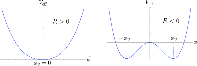
Figure 1: The effective potential $V_{\rm eff}=-\xi R\phi^{2}/2+V_{0}|\phi|^{\frac{10}{3}}$ with $\xi<0$ and $V_{0}>0$. The left panel [unbroken phase] corresponds to the effective potential with a positive value of the curvature scalar $R$, while the right one [broken phase] is a case of $R<0$.

Now we turn to an issue related to the spontaneous breaking of the conformal symmetry. We notice that the spontaneous symmetry breaking can be realized for a negative value of the curvature scalar with $R<0$ and $V_{0}>0$. To see this, we consider an effective potential $V_{\rm eff}$ for the canonical scalar field ($\omega=1$) and $V_{0}>0$ in the action (1.1) as

$$V_{\rm eff}=-\frac{1}{2}\xi\phi^{2}R+V_{0}|\phi|^{\frac{10}{3}}.$$ (3.13)

As was mentioned in Eq.(1.2), here $\xi$ is fixed as a negative value of $\xi=-3/16$ for the canonical scalar $\omega=1$, which preserves the conformal symmetry of the action (1.1). Since the solution $(i)$ ($V_{0}=0$) with a stable equilibrium $\phi_{v}=0$ does not provide a symmetry-broken phase, we focus on the case $(ii)$ with $\epsilon=1$ giving $V_{0}>0$ (hereafter we fix $\epsilon=1$).

It turns out that for $(ii)$ with the positive 5D curvature scalar $R>0$, we have only one vacuum solution of $\phi_{v}=0$, while for $R<0$, there exist two vacua of $\pm\phi_{v}$ with non-zero value:

$$\phi_{v}=e^{\frac{3}{2}\mu^{2}y_{*}^{2}}\phi_{0},$$ (3.14)

where $y_{*}$ is given by $y_{*}=4y_{0}/3\pm\sqrt{3/\mu^{2}+16y_{0}^{2}}/3$. In this case, the conformal symmetry is spontaneously broken with the symmetry breaking scale $\phi_{v}$ given by (3.14). This result is summarized in Fig.1 which shows that the effective potential with $R>0$ has only one minimum $\phi_{v}=0$ ($left$), while for $R<0$, it has two minima with $\pm\phi_{v}$ ($right$) which corresponds to the case of spontaneous breaking of the conformal symmetry.

4 Tensor perturbation

In this section, we explore the stability of the solution $(i),~{}(ii)$ by performing a tensor fluctuation around the solutions. Note that the impact of conformal invariance shows up in the perturbation theory. One can always go to the unitary gauge and choose $\varphi=0$ in the scalar perturbation with $\phi=\phi_{0}+\varphi$. On the other hand, when $\omega/\xi\neq-16/3,$ it is no longer possible to gauge away the fluctuation, and $\varphi$ is a dynamical field coupled to other fluctuations.

To investigate a tensor fluctuation around the solutions $(i),(ii),$ we need to consider the tensor perturbation of the metric as

$$ds^{2} = a^{2}(\eta_{\mu\nu}+h_{\mu\nu})dx^{\mu}dx^{\nu}+N^{2}dy^{2}$$ (4.1)

$$= a^{2}\Big{[}(\eta_{\mu\nu}+h_{\mu\nu})dx^{\mu}dx^{\nu}+dz^{2}\Big{]},$$ (4.2)

where a new variable $z$ given in a conformally flat metric (4.2) satisfies $Ndy=adz$. It is found the equation of motion for the tensor modes $h_{\mu\nu}$ is given by

$$\partial_{z}^{2}h_{\mu\nu}+A(z)\partial_{z}h_{\mu\nu}-\Box^{(4)}h_{\mu\nu}=0,$$ (4.3)

where $h_{\mu\nu}$ satisfy the transverse-traceless gauge conditions ($\partial^{\mu}h_{\mu\nu}=0$, $h=\eta^{\mu\nu}h_{\mu\nu}=0$) and $A(z)$ is given by

$$A(z)=\frac{3}{a}\frac{\partial a}{\partial z}+\frac{2}{\phi}\frac{\partial\phi}{\partial z}.$$ (4.4)

Consideration of a separation of variables $h_{\mu\nu}(x,z)=f(z)H_{\mu\nu}(x)$ splits the equation (4.3) into two parts:

$$[-\partial_{z}^{2}+V_{\rm QM}]f=m^{2}f,$$ (4.5)

$$\Box^{(4)}H_{\mu\nu}=m^{2}H_{\mu\nu}.$$ (4.6)

Here $m$ is the mass of four dimensional Kaluza-Klein modes and the corresponding quantum mechanical potential $V_{\rm QM}$ reads

$$V_{\rm QM}=\frac{1}{2}\frac{\partial A}{\partial z}+\frac{A^{2}}{4}.$$ (4.7)

One can check easily that $V_{\rm QM}$ vanishes for solution $(i)$, which yields just plane wave solution with constant zero mode. On the other hand, for solution $(ii)$, it gives an inverse square potential as

$$V_{\rm QM}=\frac{15}{4z^{2}},$$ (4.8)

where the corresponding Hamiltonian can be written as

$$H=\frac{1}{2}(p_{z}^{2}+gz^{-2})~{}~{}~{}{\rm with}~{}g=\frac{15}{4}.$$ (4.9)

It is known in [17, 18] that for the Schrödinger equation (4.5) with the inverse square potential ($V_{\rm QM}=g/z^{2}$), the stability of the mode $f$ is determined by the condition

$$g>-\frac{1}{4},$$ (4.10)

which guarantees that the graviton mode along the fifth dimension with $g=15/4$ is stable.

Before closing the section, we remark that the graviton mode along the fifth dimension preserves the residual conformal $SO(2,1)$ symmetry. It is well-known that the quantum mechanical system of the Hamiltonian (4.9) is conformally invariant [20], being reffered to as conformal quantum mechanics (CQM). To see this, we first construct the CQM action for $H$ (4.9) from the Lagrangian formalism:

$$S_{\rm CQM}=\frac{1}{2}\int dt\Big{(}\dot{z}^{2}-\frac{g}{z^{2}}\Big{)},$$ (4.11)

which is invariant under the non-relativistic conformal transformations:

$$t^{\prime}=\frac{\alpha t+\beta}{\gamma t+\delta},~{}~{}~{}z^{\prime}=\frac{z}{\gamma t+\delta}~{}~{}~{}~{}~{}{\rm with}~{}~{}~{}\alpha\delta-\beta\gamma=1.$$ (4.12)

In this case, it is known that three generators, i.e., $H$ (time translation), $D$ (dilatation), $K$ (special conformal) generators can act with the transformation rules:

$$H;~{}~{}~{}t^{\prime}=t+\tilde{t},~{}~{}~{}~{}~{}~{}~{}D;~{}~{}~{}t^{\prime}={\tilde{d}}^{2}t,~{}~{}~{}~{}~{}~{}~{}K;~{}~{}~{}t^{\prime}=\frac{t}{\tilde{k}t+1},$$ (4.13)

where $\tilde{t},~{}\tilde{d},~{}\tilde{k}$ are some constants and the generators $D$ and $K$ at $t=0$ in addition to $H$ (4.9) are given by

$$D=-\frac{1}{4}(zp_{z}+p_{z}z),~{}~{}~{}K=\frac{1}{2}z^{2}.$$ (4.14)

These generators obey $SO(2,1)$ commutations rules given by

$$[H,D]=iH,~{}~{}~{}~{}~{}[K,D]=iK,~{}~{}~{}~{}~{}[H,K]=2iD,$$ (4.15)

whose Casimir invariant ${\cal C}$ is given by ${\cal C}=(HK+KH)/2-D^{2}=3/4$.

5 Summary and discussion

In this paper, we considered the conformally invariant gravity in 5D, which consists of a scalar field nonminimally coupled to the curvature with its potential. We found two solutions $(i)$ and $(ii)$ giving 4D Minkowski vacuuum. By analyzing the dynamics of the metric perturbations around the solutions, we showed that two solutions are stable, since the former yields a plane wave solution with the constant zero mode, whereas the latter gives an inverse square potential. In particular, it was shown for the solution $(ii)$ that one has unbroken phase when $R>0$, $V_{0}>0$, while for $R<0$, $V_{0}>0$ the spontaneous breaking of the conformal symmetry can be realized with the scale $\phi_{v}$ given by (3.14).

We point out that the solution $(ii)$ may lead to a different mechanism which allows the possibility of a spontaneous breaking of translational invariance along the extra dimension. To this end, we consider a solution explicitly to Eq.(4.5) for $m^{2}=0$ as

$$f(z)_{m^{2}=0}=c_{1}z^{\frac{5}{2}}+c_{2}z^{-\frac{3}{2}}$$ (5.1)

with arbitrary constants $c_{1}$ and $c_{2}$. The first term of the $r.h.s$ in Eq.(5.1) is not normalizable since the function $f(z)$ diverges at infinity, while the second term can not lead to a normalizable solution due to its divergence at the origin. Thus, there is no normalizable zero mode solution. To resolve this problem, we define a new evolution operator ${\cal R}$ [20] given in terms of $K$ (4.14) and $H$ (4.9)

$${\cal R}\equiv\frac{1}{2}\Big{(}\frac{1}{a}K+aH\Big{)},$$ (5.2)

which yields the eigenvalues of ${\cal R}$ as follows

$$r_{n}=r_{0}+n,~{}~{}~{}~{}~{}~{}~{}r_{0}=\frac{3}{2}.$$ (5.3)

Here, $a$ is some constant with the length dimension. It turns out that the new evolution operator ${\cal R}$ (5.2) provides a normalizable ground state $f_{0}$:

$$f_{0}(z)=c_{0}z^{\frac{5}{2}}e^{-\frac{z^{2}}{2}},~{}~{}~{}~{}z\geq 0,$$ (5.4)

where a constant $c_{0}$ is given by $c_{0}=1$, being obtained from the normalization condition $\int_{0}^{\infty}|f_{0}(z)|^{2}dz=1$. Importantly, even if we have the normalizable ground state (5.4) by introducing the new evolution operator ${\cal R}$ (5.2), it implements the spontaneous breaking of the conformal symmetry in the sense that the fundamental length scale $a$ is not included in the Lagrangian but generated by the particular form of the vacuum. On the other hand, it should be pointed out that since the well-defined ground state described by the Hamiltonian $H$ which generates the time-translation is not present, it may lead a spontaneous symmetry breaking of time-translational invariance along the dynamical fifth direction[21, 22, 23, 24].

We conclude with the following remark. We see that both solutions $(i)$ and $(ii)$ can be characterized by Gaussian warp factor [25, 26, 27], where the maximum value is located at $y=0$ and $y=y_{0}$, respectively. But, the vacuum mode $\phi_{v}$ of Eq. (3.14) of the scalar field and the massless mode of gravity for the broken phase ($R<0$, $V_{0}>0$) are not localized on the Gaussian brane, because a value of $y_{*}$ in (3.14) can not be equivalent to $y_{0}$ and the zero mode (5.1) is written as $f(y)_{m^{2}=0}=\tilde{c}_{1}e^{-5\mu^{2}y_{0}y}+\tilde{c}_{2}e^{3\mu^{2}y_{0}y}$ in $y$-coordinate. Thus, it seems to be hard to describe the brane-world scenario with the current approach. One possible alternative to apply our result to the scenario would be to treat the conformal gravity discussed in this study (or its variation) as the conformal matter sector and introduce 5D Einstein-Hilbert action separately. Then, there could be a possibility of addressing some of the related issues, especially the brane stabilization as a consequence of the spontaneous symmetry breaking. The details will be reported elsewhere.

References

- [1] H. Weyl, Sitzungsber. Preuss. Akad. Wiss. Berlin (Math. Phys. ) 1918 (1918) 465; H. Weyl, Annalen Phys. 59 (1919) 101 [Surveys High Energ. Phys. 5 (1986) 237] [Annalen Phys. 364 (1919) 101]. doi:10.1002/andp.19193641002
- [2] P. A. M. Dirac, Proc. Roy. Soc. Lond. A 165 (1938) 199. doi:10.1098/rspa.1938.0053; P. A. M. Dirac, Proc. Roy. Soc. Lond. A 333 (1973) 403. doi:10.1098/rspa.1973.0070.
- [3] R. Jackiw and S.-Y. Pi, J. Phys. A 44 (2011) 223001. doi:10.1088/1751-8113/44/22/223001 [arXiv:1101.4886 [math-ph]]; See also T. Y. Moon, J. Lee and P. Oh, Mod. Phys. Lett. A 25, 3129 (2010). doi:10.1142/S0217732310034201 [arXiv:0912.0432 [gr-qc]] and references therein.
- [4] T. Padmanabhan, Class. Quant. Grav. 2 (1985) L105. doi:10.1088/0264-9381/2/5/002.
- [5] D. A. Demir, Phys. Lett. B 584 (2004) 133. doi:10.1016/j.physletb.2004.01.044 [hep-ph/0401163].
- [6] O. Bertolami and C. Carvalho, Phys. Rev. D 74, 084020 (2006). doi:10.1103/PhysRevD.74.084020 [gr-qc/0607043].
- [7] O. Bertolami and C. Carvalho, Phys. Rev. D 76, 104048 (2007). doi:10.1103/PhysRevD.76.104048 [arXiv:0705.1923 [hep-th]].
- [8] N. Arkani-Hamed, S. Dimopoulos and G. R. Dvali, Phys. Lett. B 429, 263 (1998). doi:10.1016/S0370-2693(98)00466-3 [hep-ph/9803315]; L. Randall and R. Sundrum, Phys. Rev. Lett. 83, 3370 (1999). doi:10.1103/PhysRevLett.83.3370 [hep-ph/9905221]; L. Randall and R. Sundrum, Phys. Rev. Lett. 83, 4690 (1999). doi:10.1103/PhysRevLett.83.4690 [hep-th/9906064]; P. D. Mannheim, “Brane-localized gravity,” Hackensack, USA: World Scientific (2005).
- [9] P. S. Wesson, “Space - time - matter: Modern Kaluza-Klein theory,” Hackensack, USA: World Scientific (2007).
- [10] J. Ponce De Leon, Mod. Phys. Lett. A 16 (2001) 2291. doi:10.1142/S0217732301005709 [gr-qc/0111011].
- [11] N. Doroud, S. M. M. Rasouli and S. Jalalzadeh, Gen. Rel. Grav. 41 (2009) 2637. doi:10.1007/s10714-009-0793-y.
- [12] S. M. M. Rasouli, M. Farhoudi and P. Vargas Moniz, Class. Quant. Grav. 31 (2014) 115002. doi:10.1088/0264-9381/31/11/115002 [arXiv:1405.0229 [gr-qc]].
- [13] S. M. M. Rasouli and P. V. Moniz, Class. Quant. Grav. 33 (2016) 035006. doi:10.1088/0264-9381/33/3/035006 [arXiv:1601.07828 [gr-qc]].
- [14] I. Bars, P. Steinhardt and N. Turok, Phys. Rev. D 89, 043515 (2014). doi:10.1103/PhysRevD.89.043515 [arXiv:1307.1848 [hep-th]].
- [15] H. Cheng, Phys. Rev. Lett. 61, 2182 (1988). doi:10.1103/PhysRevLett.61.2182.
- [16] K. M. Case, Phys. Rev. 80, 797 (1950). doi:10.1103/PhysRev.80.797.
- [17] F. Calogero, J. Math. Phys. 10 (1969) 2191. doi:10.1063/1.1664820.
- [18] S. Moroz, Phys. Rev. D 81, 066002 (2010). doi:10.1103/PhysRevD.81.066002 [arXiv:0911.4060 [hep-th]].
- [19] P. Breitenlohner and D. Z. Freedman, Phys. Lett. B 115 (1982) 197. doi:10.1016/0370-2693(82)90643-8.
- [20] V. de Alfaro, S. Fubini and G. Furlan, Nuovo Cim. A 34 (1976) 569. doi:10.1007/BF02785666.
- [21] S. Fubini, Nuovo Cim. A 34 (1976) 521. doi:10.1007/BF02785664.
- [22] E. D’Hoker and R. Jackiw, Phys. Rev. Lett. 50, 1719 (1983). doi:10.1103/PhysRevLett.50.1719.
- [23] C. W. Bernard, B. E. Lautrup and E. Rabinovici, Phys. Lett. B 134 (1984) 335. doi:10.1016/0370-2693(84)90011-X.
- [24] E. Rabinovici, Lect. Notes Phys. 737 (2008) 573 [arXiv:0708.1952 [hep-th]].
- [25] E. E. Flanagan, S. H. H. Tye and I. Wasserman, Phys. Lett. B 522 (2001) 155. doi:10.1016/S0370-2693(01)01261-8 [hep-th/0110070].
- [26] J. Alexandre and D. Yawitch, Phys. Lett. B 676 (2009) 184. doi:10.1016/j.physletb.2009.05.003 [arXiv:0812.1307 [gr-qc]].
- [27] I. Quiros and T. Matos, arXiv:1210.7553 [gr-qc].