Effects of Competition and Cooperation Interaction between Agents on Networks in Presence of a “Market Capacity”.

Abstract

A network effect is introduced taking into account competition, cooperation and mixed-type interaction amongst agents along a generalized Verhulst-Lotka-Volterra model. It is also argued that the presence of a “market capacity” enforces an indubious limit on the agent’s size growth. The state stability of triadic agents, i.e., the most basic network plaquette, is investigated analytically for possible scenarios, through a fixed point analysis. It is discovered that: (i) “market” demand is only satisfied for full competition when one agent monopolizes the market; (ii) growth of agent size is encouraged in full cooperation; (iii) collaboration amongst agents to compete against one single agent may result in the disappearance of this single agent out of the market, and (iv) cooperating with two “rivals” may become a growth strategy for an intelligent agent.

1 INTRODUCTION

Complex Networks and Multi-Agent Systems, are very active fields of research. They entail the study of networks of interacting agents whose structure is irregular, complex and dynamically evolving with time [2, 1, 3, 4]. Most real systems in biology, chemistry, engineering, socioeconomics, are made up of millions and millions of interacting agents (i.e atoms, electrons, people as the case may be) which account for fluctuations in the overall behaviour of the system. Over the years, it has also been discovered that non-linear mathematical models replicate the dynamics of real systems better than the linear ones [5, 6]. An example of such former models is the Lotka-Volterra model [7, 8], and its generalisation [9, 10, 12, 11, 13, 14, 15, 16, 18, 17, 19], which is also known as the prey-predator model [20].

The Lotka-Volterra model has been used in various ways to model complex systems[9, 10, 12, 11, 13, 14, 15, 16]. For instance, in [12], the model was used in e-commerce web sites in a competitive scenario to explore its effects and the characteristic of “rich gets richer” on Internet economy, and the “winner-takes-all” phenomenon. This was an improvement on [13, 14] where interacting agents where discovered to be “sharing the market”. The Verhulst-Lotka-Volterra model was generalized in [17] through the introduction of a non-linear, symmetric interaction function, used to investigate a competitive scenario. This resulted in a self-organising clustering of agents, which were either chaotic or/and non chaotic in nature as a result of their dependence on the agent’s size and their initial state conditions. Cooperative scenarios examined in [18] were modeled individually without imposing any “market condition”. This resulted in the growth of different clusters of interacting agents beyond their capacity in contrast to the competitive case. A complex network representation of the competitive and the cooperative scenarios was presented in [19], in order to give another description of some generalized Verhulst-Lotka-Volterra model.

This present paper offers new insights on the effects of competitive and/or cooperative interaction in a multi-agent system when $n$ agents have some common resources to share in the “market”.

The main contribution of our paper is two folds: firstly, we generalize the Verhulst-Lotka-Volterra model by introducing a network effect through an undirected but weighted graph. The weights suitably represent competition or cooperation. The elements of the resulting adjacency matrix replaces the strength parameter in the interaction function of the[17, 18] model in order to enable a mixed-type of interactions, i.e., having a system in which competitive and cooperative scenarios are considered to occur simultaneously amongst the various interacting agents.

Secondly, we introduce a market capacity in the model to replace individual agent’s capacity: this is a realistic constraint, i.e., the maximum level which all the agents may reach in the market, like in Verhulst model of limited population growth [22, 23]- thereby enforcing a natural (endogenous) limit on agent’s size growth.

Such competition, cooperation and mixed-type of interactions are analyzed below for triad interacting agents through the evaluation of the eigenvalues of the relevant Jacobian matrix computed at corresponding fixed points, in order to investigate the system stability. This triad system has been chosen as the most simple yet complex enough as representative of basic networks [21]. Notice that the model goes well away for the 2-player prisoner (dilemma) game.

Thus, a mixed-type of interactions between agents, made possible through the network effect in the generalized Verhulst-Lotka-Volterra model, markedly differs from previous works [17, 19, 18], and seems more realistic.

This paper is organized as follows: in Section 2, the generalized Verhulst-Lotka-Volterra model is discussed. Section 3 contains the outline of the mathematical model used in this paper. The fixed point analysis and state stability are investigated in Section 4. In Section 5, initial size conditions and convergence to a steady state of the triad interacting agents are further illustrated through simulations. We demonstrate the presence of growth and/or decay effects in various scenarios, - sometimes rather complex, but a posteriori understandable. The paper is concluded in Section 6. It appears that the model is suitable for describing not only an “economic market” but other agent based cases such as co-autorship, or more generally team working, or any other small or large network based complex systems.

2 THE GENERALIZED VERHULST-LOTKA-
VOLTERRA MODEL

A generalized Verhulst-Lotka-Volterra Model introduced in [17] is given by:

$$\dot{s_{i}}=\alpha_{i}s_{i}(\beta_{i}-s_{i})-\sum_{i\neq j}\gamma(s_{i},s_{j})s_{i}s_{j},\quad\quad\quad i=1,\ldots,n,$$ (2.1)

where $s_{i}$ is the size of agent $i$ such that $0\leq s_{i}\leq 1$; $\dot{s_{i}}$ is its time derivative; $\alpha_{i}$ is agent’s growth rate if no interaction is present, $\beta_{i}$ is the agent’s maximum capacity and $\gamma(s_{i},s_{j})$ is the interaction function. The first term is a Verhulst-like term [22, 23] and the others stem from the Lotka-Volterra model [7, 8].

The interaction function $\gamma(s_{i},s_{j})$ is defined by

$$\gamma(s_{i},s_{j})=K\exp\left[-\left(\frac{s_{i}-s_{j}}{\sigma}\right)^{2}\right];$$ (2.2)

it is a continuously differentiable function that allows a proper theoretical analysis of the system dynamics leading to conclusions which will appear to be likely model independent. The positive parameter $\sigma$ controls or scales the intensity of agent size similarity and the parameter $K$ determines the scenarios of agent’s interaction.

The model is used in [17] to analyze a system of $n$ agents in competition for some common resources with competition becoming more aggressive between agents with similar size. This is because as $|s_{i}-s_{j}|\rightarrow 0$, the interaction function $\gamma(s_{i},s_{j})\rightarrow K$ for a constant parameter $\sigma$, its maximum value. The competition weakens when agents have distinctly different sizes, thereby suggesting a peer-to-peer competition modelling.

For the peer-to-peer interaction system, presented in [17, 18], a strength parameter $K$ was introduced: $K>0$ was considered to show the presence of competition in the market, while $K<0$ implied cooperation. Under the cooperative scenario, the interaction function is defined in the interval $-K<\gamma(s_{i},s_{j})<0$. In order to avoid complexity and instability of the system, the value of $K$ was chosen carefully through fixed point analysis of agents with equal sizes[18], whose eigenvalues are

$$\lambda_{1,\ldots,n}=\frac{K-1}{1+(n-1)K},$$ (2.3)

so that, the $K$ range interval $-\frac{1}{n-1}<K<0$ ensures the stability of the system.

3 THE MODEL

This paper is a study of the Verhulst-Lotka-Volterra model when competition and cooperation can occur between linked agents. The market capacity $\beta$ becomes the amount of product/service sales that could be reached within a certain period of time by any agents in the “market” [24]. The relationship between the individual agent’s maximum capacity $\beta_{i}$ and $\beta$ is given by:

$$\beta_{i}=\beta-\sum_{i\neq j}s_{j},$$ (3.1)

so that the initial Verhulst-Lokta-Volterra model becomes:

$$\alpha_{i}s_{i}(\beta_{i}-s_{i})=\alpha_{i}s_{i}\left(\beta-\sum_{i=1}s_{i}\right).$$ (3.2)

In addition, interaction among agents is introduced and modeled by a matrix K with elements $k_{ij}=k_{ji}$, which are zero on the diagonal, and can be +1 or -1 off the diagonal. Thus, the interaction function becomes:

$$\gamma(s_{i},s_{j})=k_{ij}\exp\left[-\left(\frac{s_{i}-s_{j}}{\sigma}\right)^{2}\right]$$ (3.3)

with $0<\gamma(s_{i},s_{j})<|k_{ij}|$.

This matrix K is the adjacency matrix of a network represented by a weighted and undirected graph. The weights are $0,-1$ and $+1$ indicate no interaction, cooperation and competition respectively. Furthermore, we assume that there is no loop, that is, an agent cannot compete or cooperate with herself. For some special matrices K, we obtain the model in [18, 17]. For instance, when

$$\scriptstyle\textbf{K}\equiv\left[\begin{array}[]{ccccc}0&1&.&.&1\\ 1&0&&.&1\\ .&&.&&.\\ .&&&.&.\\ 1&1&.&.&0\end{array}\right]$$

we obtain the full competitive scenario as in [17]. For

$$\scriptstyle\textbf{K}\equiv\left[\begin{array}[]{ccccc}0&-1&.&.&-1\\ -1&0&&.&-1\\ .&&.&&.\\ .&&&.&.\\ -1&-1&.&.&0\end{array}\right],$$

this is the full cooperative scenario [18]. In addition the network matrix

$$\scriptstyle\textbf{K}\equiv\left[\begin{array}[]{ccccc}0&k_{12}&.&.&k_{1n}\\ k_{21}&0&&.&k_{2n}\\ .&&.&&.\\ .&&&.&.\\ k_{n1}&k_{n2}&.&.&0\\ \end{array}\right]$$

ensures a mixed-type of interaction amongst the agents in the model, when $k_{ij}(=k_{ji})$ takes the value +1 or -1. That is, when competition and cooperation occur simultaneously amongst interacting agents in the system. For example, for $n=3$, in our model, we can have two agents collaborating in order to compete effectively with the third agent. This can be compared with the case of two small companies collaborating to compete against a big company which had previously monopolized the market or when two political parties merge together for the purpose of winning over a ruling (or over a potentially ruling) party in an election or when scientific teams or authors cooperate on some research topics.

Thus suppose that there exist $n$ agents sharing some common resources. Let us assume that agents increase in size if they acquire some portion of the resources or have their size reduced if any market portion is lost. Our mathematical model is defined by an $n$-dimensional differential equation:

$$\dot{s}_{i}=\alpha_{i}s_{i}\left(\beta-\sum_{i=1}^{n}s_{i}\right)-\sum_{i\neq j}k_{ij}\exp\left[-\left(\frac{s_{i}-s_{j}}{\sigma}\right)^{2}\right]s_{i}s_{j},\quad\quad\quad\quad i=1,\ldots,n$$ (3.4)

where $s_{i}$ is the agent size such that $0<s_{i}\leq 1$; $\dot{s}$ is its time derivative; $\alpha_{i}$ is the growth rate of agent $i$ if no interaction is present; $\beta$ is the market capacity and $k_{ij}$ is the element of the network matrix K which determines the interaction between agent $i$ and $j$. The interaction function $\gamma(s_{i},s_{j})$ is composed of dynamic parameters that result from the difference between agents in relation; the parameter $\sigma$ is a positive parameter that regulates the difference in the agent’s size. Note that while K indicates what interaction is present, $\sigma$ determines the “range” of interaction of the agents. Indeed, in contrast to the “large” interaction between equal size agents, the intensity of interactions between “agents with bigger market share” and “those with small market share” occurs to be weak, since as $\mid s_{i}-s_{j}\mid\rightarrow\infty$, the interaction function $\gamma(s_{i},s_{j})\rightarrow 0$; on the contrary, indeed, as $\mid s_{i}-s_{j}\mid\rightarrow 0$, $\gamma(s_{i},s_{j})\rightarrow\pm 1$ depending on $k_{ij}$, which signifies a strong interaction between agents with similar sizes.

For the sake of simplicity, without much losing generality, it can be assumed that the agents have the same dynamic properties $\alpha_{i}=1$, while the market capacity can be $\beta=1$. Therefore, equation (3.4) becomes:

$$\dot{s}_{i}=s_{i}\left(1-\sum_{i=1}^{n}s_{i}\right)-\sum_{i\neq j}k_{ij}\exp\left[-\left(\frac{s_{i}-s_{j}}{\sigma}\right)^{2}\right]s_{i}s_{j},\quad\quad\quad\quad i=1,\ldots,n$$ (3.5)

where, as stated earlier, $k_{ij}$, $i,j=1,\ldots,n$ are elements of the interaction matrix K.

4 FIXED POINT ANALYSIS AND STABILITY

In this section, the fixed point analysis of the model is done in order to investigate the stability of the system for all scenarios. A triad system of agent (i.e. $n=3$) was chosen as a simple yet complex representative of a basic network, in order to illustrate some of the properties of the model analytically.

Suppose $A_{1},A_{2}$ and $A_{3}$ are triad interacting agents with market sizes ${s}_{1},{s}_{2}$ and ${s}_{3}$ respectively, from equations (3.3) the system of triads becomes:

$$\dot{s}_{1} = s_{1}(1-s_{1}-s_{2}-s_{3})-k_{12}\exp^{-\left(\frac{s_{1}-s_{2}}{\sigma}\right)^{2}}s_{1}s_{2}-k_{13}\exp^{-\left(\frac{s_{1}-s_{3}}{\sigma}\right)^{2}}s_{1}s_{3},$$ (4.1)

$$\dot{s}_{2} = s_{2}(1-s_{1}-s_{2}-s_{3})-k_{12}\exp^{-\left(\frac{s_{2}-s_{1}}{\sigma}\right)^{2}}s_{2}s_{1}-k_{23}\exp^{-\left(\frac{s_{2}-s_{3}}{\sigma}\right)^{2}}s_{2}s_{3},$$ (4.2)

$$\dot{s}_{3} = s_{3}(1-s_{1}-s_{2}-s_{3})-k_{13}\exp^{-\left(\frac{s_{3}-s_{1}}{\sigma}\right)^{2}}s_{3}s_{1}-k_{23}\exp^{-\left(\frac{s_{3}-s_{2}}{\sigma}\right)^{2}}s_{3}s_{2}.$$ (4.3)

The possible K-matrices for describing the different scenarios of interaction amongst the agents $A_{1},A_{2}$ and $A_{3}$ are:

$$\scriptstyle\textbf{K}_{1}=\left[\begin{array}[]{ccccc}0&1&1\\ 1&0&1\\ 1&1&0\\ \end{array}\right],\textbf{K}_{2}=\left[\begin{array}[]{ccccc}0&1&1\\ 1&0&-1\\ 1&-1&0\\ \end{array}\right],\textbf{K}_{3}=\left[\begin{array}[]{ccccc}0&-1&-1\\ -1&0&1\\ -1&1&0\\ \end{array}\right],\textbf{K}_{4}=\left[\begin{array}[]{ccccc}0&-1&-1\\ -1&0&-1\\ -1&-1&0\\ \end{array}\right]$$

where $\textbf{K}_{1}$ represents the matrix for a full competitive system with three interacting agents; $\textbf{K}_{2}$ is a matrix for mixed-type of interaction system, where one agent compete with two other agents in cooperation. In this case, agent $A_{1}$ competes with agent $A_{2}$ and agent $A_{3}$ which are in cooperation. $\textbf{K}_{3}$ is a matrix for mixed-type of interaction system, where one agent cooperates with two other agents in competition, in this case, agent $A_{1}$ cooperates with agent $A_{2}$ and agent $A_{3}$ which are in competition with each other. $\textbf{K}_{4}$ represents the matrix for a full cooperative system amongst the three interacting agents. It can be observed that other cases of the mixed-type of interaction are isomorphic to the ones here presented.

The fixed point analysis of the system entails the evaluation of the eigenvalues of the relevant Jacobian matrix computed at each corresponding fixed point, thus used to determine the stability of the system. When the real part of all the eigenvalues is negative, the system is said to be stable. If at least one eigenvalue has a positive real part, the system is unstable.

4.1 Fully Competitive and Fully Cooperative Scenario

In this paragraph, the stability of the system under either the fully competitive or fully cooperative scenarios is discussed, that is, the model with network matrix $\textbf{K}_{1}$ and $\textbf{K}_{4}$. By definition, a fixed point is a point in the phase space where all the time derivatives are zero, i.e., $\dot{s}_{i}=0$ for $i=1\ldots,n$. The following fixed points were detected analytically from equations (4.1)- (4.3):

1. $s_{i}=0$ for $i=1,2,3$. i.e. all agents with zero size.

2. $s_{i}=1$ and $s_{j}=0$ for every $i\neq j$ i.e. one agent monopolizes the market.

3. $s_{i}=b$ for $i=1,2,3$, $0<b\leq 1$. i.e. all agents own an equal share of the market.

Moreover it can be easily shown that the elements of the Jacobian matrix of the triads are:

$$[J]_{(i,k)}=\frac{\partial\dot{s_{i}}}{\partial s_{k}}=\left\{\begin{array}[]{ll}1-2s_{i}-\sum_{i\neq j}s_{j}\left(1+\gamma(s_{i},s_{j})\left[1-\frac{2}{\sigma^{2}}s_{i}(s_{i}-s_{j})\right]\right),&\hbox{ for $k=i$;}\\ \\ -s_{i}-s_{i}\gamma(s_{i},s_{k})\left[1-\frac{2}{\sigma^{2}}s_{k}(s_{i}-s_{k})\right],&\hbox{for $k\neq i$,}\end{array}\right.$$

from which the stability conditions are to be found at each fixed point.

Type (I) Fixed Point

The type (I) fixed point analysis is the case in which all agents have size zero, i.e., $s_{i}=0$ for $i=1,2,3$. The evaluated Jacobian matrix at the type (I) fixed point, is given by:

$$\textbf{J}=\left[\begin{array}[]{ccccc}1&0&0\\ 0&1&0\\ 0&0&1\\ \end{array}\right]$$

whose eigenvalues are all equal to 1 (i.e., $\lambda_{1}=\lambda_{2}=\lambda_{3}=1$). Therefore, it is an unstable fixed point. At this fixed point, competition or cooperation is not applicable since all agents are at level zero. In other words, these results do not depend on the network matrix $K$.

Type (II) Fixed Point

The type (II) fixed point analysis corresponds to the case in which one agent eventually monopolizes the market and satisfies the whole demand (i.e., $s_{1}=1$); all others have size zero (i.e., $s_{2}=s_{3}=0$). Evaluating the Jacobian matrix at the type (II) fixed point, we obtain:

$$\textbf{J}=\left[\begin{array}[]{ccccc}-1&-1-\phi_{12}&-1-\phi_{13}\\ 0&-\phi_{12}&0\\ 0&0&-\phi_{13}\\ \end{array}\right],$$

where $\phi_{ij}=k_{ij}\exp(-\sigma^{-2})$, for $i,j=1,2,3$ and $i\neq j$. The eigenvalues are obtained from

$$(-1-\lambda)(-\phi_{12}-\lambda)(-\phi_{13}-\lambda)=0$$

which implies that $\lambda_{1}=-1$, $\lambda_{2}=-\phi_{12}$ and $\lambda_{3}=-\phi_{13}$.

In the fully competitive scenario, all $k_{ij}=1$ for $i\neq j$, thereby resulting to an all negative eigenvalues of J. Indeed, this implies stability of the system at this fixed point. This is applicable in real systems: if an agent monopolises the competitive market, the agent will ensure that such a domination is not lost, whence keeping the market stable.

On the contrary, in the fully cooperative scenario, $\lambda_{2}$ and $\lambda_{3}$ are positive, since all $k_{ij}=-1,i\neq j$, thereby making the system unstable. This is also realistic, since in cooperation, the ultimate goal is the maximisation of all agents gain in the market. Therefore, it can be emphasized that monopoly and cooperation are not compatible terms. This accounts for systemic instability.

In conclusion, the type (II) fixed point is stable in a full competitive scenario because of the possibility of monopoly, but is unstable under full cooperation.

Type (III) Fixed Point

The type (III) fixed point analysis is the case in which all agents are eventually owning the same share of the market, i.e., $s_{i}=b$ for $i=1,2,3$, $0<b<1$. When evaluating the Jacobian matrix at this fixed point, the constant $b$ has first to be calculated by substituting $s_{i}=b$ and $\dot{s}_{i}=0$ into Equations (4.1)-(4.3). From (4.1), it can be deduced that:

$$0 = b(1-3b)-(k_{12}+k_{13})b^{2}$$ (4.4)

$$= 1-b(3+(k_{12}+k_{13}).$$ (4.5)

Therefore,

$$b=\frac{1}{(3+(k_{12}+k_{13}))}.$$ (4.6)

Similarly from (4.2) and (4.3) respectively, the following is obtained:

$$b=\frac{1}{(3+(k_{12}+k_{23}))}.$$ (4.7)

$$b=\frac{1}{(3+(k_{13}+k_{23}))}.$$ (4.8)

Therefore, from equations (4.6)-(4.8), it can be deduced that in a fully competitive system (i.e. $k_{12}=k_{13}=k_{23}=1$), the agent size is $b=\frac{1}{5}$. This implies that the aggregate size of the three agents does not reach the market maximum possible capacity, which may be the negative result of the competition amongst peers.

Thus, for a full competition of agents with the same size, the Jacobian matrix with $b=\frac{1}{5}$ is:

$$\textbf{J}=\frac{1}{5}\left[\begin{array}[]{ccccc}-1&-2&-2\\ -2&-1&-2\\ -2&-2&-1\\ \end{array}\right],$$

the eigenvalues are obtained from the characteristic polynomial

$$(-1-\lambda)^{3}-12(-1-\lambda)-16 = 0$$

The solution to the above cubic equation is $\lambda_{1}=\lambda_{2}=1$ and $\lambda_{3}=-5$. This shows that the system is unstable at this fixed point. When all the agents have an equal size in a competitive market, the system will be unstable; because the major goal of each agent is to $individually$ dominate the market. According to the model, agents with “similar” sizes are strongly interacting; this leads to a “survival of the fittest” scenario in such a competitive system, - thereby making the system unstable.

In contrast, for a cooperative system (i.e. $k_{12}=k_{13}=k_{23}=-1$), we have $b=1$, that is, collaboration makes all agents reach the market full capacity with agent sizes as a function of time possibly intersecting one another.

The corresponding Jacobian matrix for the cooperative system with $b=1$ is:

$$\textbf{J}=\left[\begin{array}[]{ccccc}-1&0&0\\ 0&-1&0\\ 0&0&-1\\ \end{array}\right];$$

the eigenvalues are obtained from the equation:

$$(-1-\lambda)^{3}=0$$

which implies that the system is stable, since $\lambda_{1,2,3}=-1.$ When all the agents with $quasi$ equal market share cooperate, with the collective goal of maximizing their profit (size) in the market, the system will definitely be stable; their goal will be achieved since the strongest possible interaction exists amongst agents with similar sizes.

It can be noted that when $b=\frac{1}{3}$, (i.e. $k_{12}=k_{13}=k_{23}=0$), there exists no interaction amongst the triads agents of equal sizes and this leads to the case whereby the agents “share the market” equally.

In conclusion to this section, a summary of the fixed point analysis of our model with the network matrix $\textbf{K}_{1}$ and $\textbf{K}_{4}$, i.e, under the fully competitive and fully cooperative scenarios is presented in Table 1. In this table, it is shown that systemic stability is observed under full competitive scenario only when one agent monopolizes the market, but under the fully cooperative scenario, stability occurs only when all the agents own an equal share of the market.

Fixed Point Analysis and Stability
Scenario	(I.) $s_{i}=0$ $\forall i$	(II.) $s_{i}=1$, $s_{j}=0$, $i\neq j$	(III.) $s_{i}=b$ $\forall i$
Full Competition	$\lambda_{1}=1$	$\lambda_{1}=-1$	$\lambda_{1}=1$
	$\lambda_{2}=1$	$\lambda_{2}=-\phi_{12}$	$\lambda_{2}=1$
	$\lambda_{3}=1$	$\lambda_{3}=-\phi_{13}$	$\lambda_{3}=-5$
	Unstable	Stable	Unstable
Full Cooperation	$\lambda_{1}=1$	$\lambda_{1}=-1$	$\lambda_{1}=-1$
	$\lambda_{2}=1$	$\lambda_{2}=-\phi_{12}$	$\lambda_{2}=-1$
	$\lambda_{3}=1$	$\lambda_{3}=-\phi_{13}$	$\lambda_{3}=-1$
	Unstable	Unstable	Stable

Table 1: Summary of analytical results under Full Competition and Full Cooperation with $\phi_{ij}=k_{ij}\exp(-\sigma^{-2})$ and $k_{ij}=\pm 1$ depending on interaction between agent $i$ and $j$.

4.2 Mixed Interaction Scenario

For the mixed interaction system of triads, two possible cases can be considered; according to the number of cooperation pairs the other cases can be easily found isomorphic to these, i.e.,

• $G_{2}$: Agent $A_{1}$ is competing both with agent $A_{2}$ and agent $A_{3}$, these two being in one cooperation scheme, i.e., the model with network matrix $\textbf{K}_{2}$. This implies that in equations (4.1)-(4.3), $k_{12}=1$, $k_{13}=1$ and $k_{23}=-1$.

• $G_{3}$: Agent $A_{1}$ cooperated with both agent $A_{2}$ and agent $A_{3}$, but these two are in competition, i.e., the model with network matrix $\textbf{K}_{3}$. Therefore, $k_{12}=-1$, $k_{13}=-1$ and $k_{23}=1$ for equations (4.1)-(4.3).

Analytically, only one fixed point was detected for the mixed interaction of triad agents which is a case of market duopoly. The coordinates of the fixed points are given by:
$s_{i}=1$, $s_{j}=1$, $s_{k}=0$, for some $i,j,k=1,2,3$, indeed, i.e. outlining the case of duopoly in a mixed interaction market.

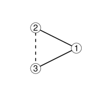
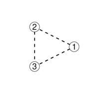
Figure 1: Graphical illustration of the four scenarios. An edge with solid line signifies a competitive interaction while an edge with dashed line signifies a cooperative interaction. Pictures respectively refers to: (a) $G_{1}$, (b) $G_{2}$, (c) $G_{3}$ and (d) $G_{4}$

Fixed point Analysis

For the fixed point analysis of the two possible mixed interaction scenarios, the Jacobian matrix is given by:

$$\textbf{J}=\left[\begin{array}[]{ccccc}-2-k_{12}&-1-k_{12}&-1-\phi_{13}\\ -1-k_{12}&-2-k_{12}&-1-\phi_{23}\\ 0&0&-1-\phi_{13}-\phi_{23}\\ \end{array}\right],$$ (4.9)

where $\phi_{ij}=k_{ij}\exp(-\sigma^{-2})$ and $i,j=1,2,3$ for $i\neq j$. Considering the two possible cases of the mixed interaction scenarios, two different Jacobian matrices emerge depending on the values of each $k_{ij}$. When one agent competes with two other agents, themselves in cooperation, $k_{12}=1$, $k_{13}=1$ and $k_{23}=-1$ which after substitution into (4.9) leads to the Jacobian matrix

$$\textbf{J}=\left[\begin{array}[]{ccccc}-3&-2&-1-\phi_{13}\\ -2&-3&-1-\phi_{23}\\ 0&0&-1-\phi_{13}-\phi_{23}\\ \end{array}\right].$$

Solving the characteristic equation

$$(-1-\phi_{13}-\phi_{23}-\lambda)[(-\lambda-3)^{2}-4]=0$$

the eigenvalues of the Jacobian matrix is obtained to be $\lambda_{1}=-5,\lambda_{2}=\lambda_{3}=-1$. This signifies systemic stability under the first case of mixed interaction scenarios with the network matrix $\textbf{K}_{2}$.

When one agent cooperates with two other agents themselves in competition with each other, $k_{12}=-1$, $k_{13}=-1$ and $k_{23}=1$; substitution into (4.9) implies that the Jacobian matrix is:

$$\textbf{J}=\left[\begin{array}[]{ccccc}-1&0&-1-\phi_{13}\\ 0&-1&-1-\phi_{23}\\ 0&0&-1-\phi_{13}-\phi_{23}\\ \end{array}\right].$$

The corresponding eigenvalues obtained from

$$(-1-\phi_{13}-\phi_{23}-\lambda)[(-1-\lambda)^{2}]=0.$$

is $\lambda_{1,2,3}=-1$. Hence, for the fixed point analysis under second possible case of mixed interaction scenario with a network matrix $\textbf{K}_{3}$ in our model, stability is observed in the system.

In conclusion of this section, for the two types of mixed interactions amongst triad agents, systemic stability is observed; this further shows the relevance of examining the co-existence of competition and cooperation amongst agents in the market.

5 SIMULATION RESULTS

In this section, we present results from numerical simulations emphasizing the initial conditions and the convertgence of triad agent sets for all interesting and possible scenarios, for each network matrix type $\textbf{K}=\{\textbf{K}_{1},\textbf{K}_{2},\textbf{K}_{3},\textbf{K}_{4}\}$.

For the sake of clarity, in Fig 1, the four possible scenarios are illustrated through undirected graphs with three vertices representing agents $A_{1},A_{2}$ and $A_{3}$ and three edges which signify the type of interaction amongst the agents. An edge with solid line signifies a competitive interaction while an edge with dashed lines signifies a cooperative interaction. Therefore, it can be deduced that in Fig 1, graph $\textbf{G}_{1}$ represents the full competitive scenario, $\textbf{G}_{2}$ represents the first case of the mixed-interactive scenario in which agent $A_{1}$ competes with $A_{2}$ and $A_{3}$, themselves in cooperation. Graph $\textbf{G}_{3}$ represents the second case of the mixed-interactive scenario in which agent $A_{1}$ cooperates with $A_{2}$ and $A_{3}$, themselves in competition and $\textbf{G}_{4}$ represents the full cooperative scenario.

We have tested different sets of initial conditions; see a few exemplary cases in Table 2. We have verified the coherence of results. This suggested to us to present only cases when the initial conditions of agents sizes are rather different or quite similar, assuming a constant parameter that controls the size similarity, $\sigma=1$. The dynamic change in agent’s size and relative behavior have been observed for each scenario. Finally, note that agent’s sizes initial conditions were chosen within a small interval in order to allow some “meaningful” interaction amongst the agents; since within our model, indeed, as $\mid s_{i}-s_{j}\mid\rightarrow\infty$, the interaction function $\gamma(s_{i},s_{j})\rightarrow 0$.

5.1 Fully Competitive Scenario ($G_{1}$)

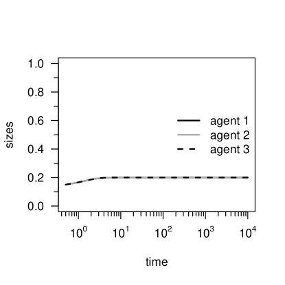
Figure 2: Fully Competitive Scenario ($G_{1}$) with different (lhs) and similar (rhs) agent’s initial sizes.

The fully competitive scenario with different initial conditions for the agent’s size is observed in Fig 2 with a consideration on dynamical change in the agent size; the market eventually ends in a monopoly. For all the permutations of the initial conditions, the agent that starts with the highest initial size, i.e $s_{0}=0.4$, eventually monopolizes the market by attaining the market capacity, while the other two agents fade out of the market. This is possible because the two agents with smaller sizes compete too weakly with the agent that eventually dominates the market.

On the contrary, when agents sizes are similar in Fig 2, the competition becomes very “fierce” and all agents are struggling for their survival in the market. After some time span, it is observed that the agents eventually have an equal share of the market; their total market share is however lower than the market capacity. Thus, strong competition among peers is shown to lead to a reduction in the aggregate output due to the selfish interest of the individual agents. Indeed, observe that the final state ($\sum s_{i}=0.6$). Convergence is generally slower in the competitive scenario when compared with the other scenarios due to the nature and effect of competition amongst the interacting agents.

5.2 Fully Cooperative Scenario ($G_{4}$)

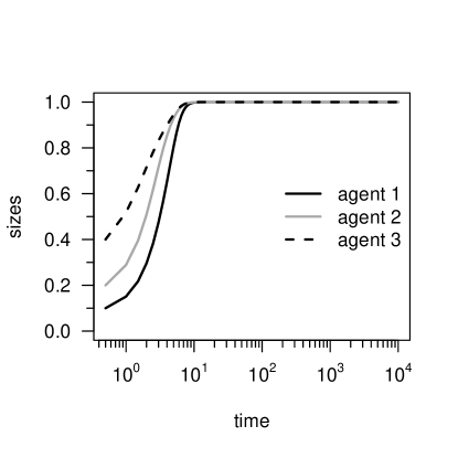
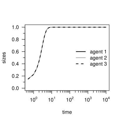
Figure 3: Fully Cooperative Scenario ($G_{4}$) with different (lhs) and similar (rhs) agent’s sizes.

The fully cooperative scenario ($G_{4}$) is analyzed for different initial sizes of the triads and illustrated in Fig 3. The cooperation amongst the agents enables all agents to grow in size up to this market capacity, thereby increasing the total market size, - which is the essence of cooperation $(\sum s_{i}>1.0)$. A simple analogy can be drawn with the case of publishing research in journals with a demand of just three papers in a journal edition (i.e. market capacity). For simplicity, let it be assumed that the three authors have the same quality standard (i.e. initial condition), under full competition, each author will have one article published making up three papers. However, the “best” situation occurs under full cooperation when each author cooperates in writing the articles; they eventually have three papers each published to their credit. Hence, the final result will be three papers for the editor and three papers for each author. One other example pertains to car owners who may own more than one car, e.g., three cars from three different manufacturers. These simple examples show that the agent’s sizes can intersect each other during full cooperation.

The simulation leads to the same effect, even if the initial conditions are permuted amongst the triads and when the agents have similar initial sizes as shown in Fig 3. Also, agents tend to ”quickly agree”, thereby converging within a short time lapse.

5.3 The single pair cooperation ($G_{2}$).

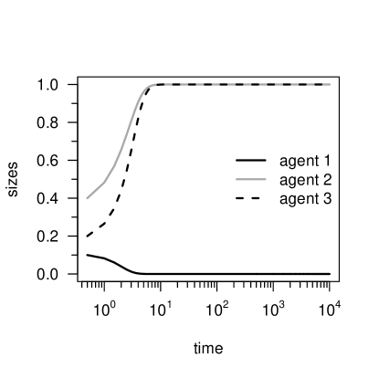
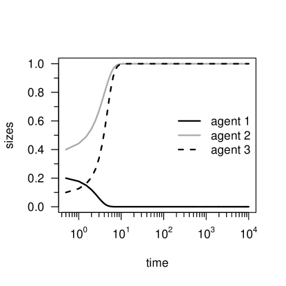
Figure 4: Mixed Interaction Scenario ($G_{2}$), $A_{1}$ competes with $A_{2}$ and $A_{3}$ in pair cooperation, for different initial sizes.

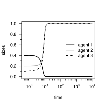
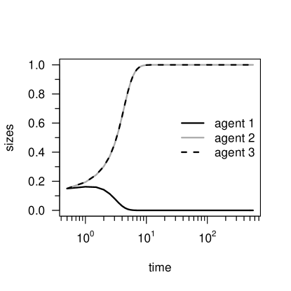
Figure 5: Mixed Interaction Scenario ($G_{2}$): $A_{1}$ competes with $A_{2}$ and $A_{3}$ in a pair cooperation, for different (lhs) or similar (rhs) initial sizes.

The mixed interaction scenario ($G_{2}$), when agent $A_{1}$ competes with agents $A_{2}$ and $A_{3}$ themselves in cooperation is shown in Fig 4 - Fig 5 for different permuted initial conditions of agent’s sizes. It can be observed that in all simulations, the sizes of agents $A_{2}$ and $A_{3}$ in cooperation grow dynamically with time up to the market capacity but agent $A_{1}$ decreases in size until it fades out of the market. The most interesting simulation is seen in Fig 5, with different initial conditions $s_{0}=\{0.4,0.2,0.1\}$ where agent $A_{1}$ initially possesses the biggest share of the market with $s_{1}=0.4$, competes with the two other agents $A_{2}$ and $A_{3}$ that alternate a smaller size $0.1$ and $0.2$. Note that the sum of the two initial shares of the cooperating agents is lower than the share of the competing agents. Interestingly, after some time, the collaboration between agents $A_{2}$ and $A_{3}$ knocks out agent $A_{1}$ from the market. An example of this scenario was experienced in 2015 in the Nigerian political history, where a political party that ruled the country for 16 years after democracy was restored, was defeated in a tight competition between the incumbent president and an aspirant that emerged from a strategic collaboration of three smaller political parties[25]. However, this is not possible if the intensity of interactions is very low amongst the agents; that is, when $A_{1}$ is “extremely bigger” in size when compared to agents $A_{2}$ and $A_{3}$.

When all the agents have similar initial conditions, the pattern is similar with agents $A_{2}$ and $A_{3}$ totally taking over the market by growing up to the market capacity as seen in Fig 5.

5.4 The double pair cooperation ($G_{3}$)

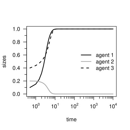
Figure 6: Mixed Interaction Scenario ($G_{3}$), $A_{1}$ cooperates with $A_{2}$ and $A_{3}$ in competition for different initial sizes.

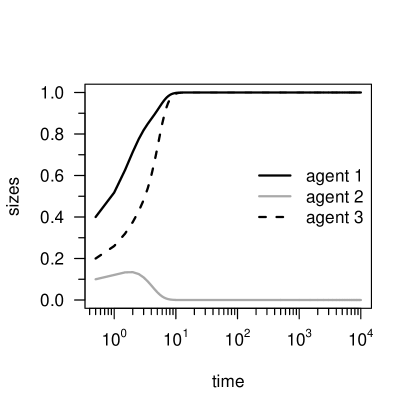
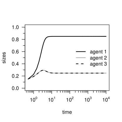
Figure 7: Mixed Interaction Scenario($G_{3}$), $A_{1}$ cooperates with $A_{2}$ and $A_{3}$ in competition for different (lhs) or similar (rhs) initial sizes.

Finally, the second possible case of mixed interaction scenario ($G_{3}$) is shown in Fig 6 - Fig 7; agent $A_{1}$ cooperates with agents $A_{2}$ and $A_{3}$ themselves in competition, for different permuted initial conditions of agent’s sizes.

Scenario	Initial Sizes $s_{i}(0)$			Growth (+) / Decay (-)
Full Competition $G_{1}$	0.1	0.2	0.4	-	-	+
	0.1	0.4	0.2	-	+	-
	0.4	0.1	0.2	+	-	-
	0.4	0.2	0.1	+	-	-
	0.2	0.4	0.1	-	+	-
	0.2	0.1	0.4	-	-	+
	0.15	0.15	0.15	+	+	+
	0.3	0.3	0.3	-	-	-
Mixed Interaction $G_{2}$	0.1	0.2	0.4	-	+	+
	0.1	0.4	0.2	-	+	+
	0.4	0.1	0.2	-	+	+
	0.4	0.2	0.1	-	+	+
	0.2	0.4	0.1	-	+	+
	0.2	0.1	0.4	-	+	+
	0.15	0.15	0.15	-	+	+
	0.3	0.3	0.3	-	+	+
Mixed Interaction $G_{3}$	0.1	0.2	0.4	+	-	+
	0.1	0.4	0.2	+	+	-
	0.4	0.1	0.2	+	-	+
	0.4	0.2	0.1	+	+	-
	0.2	0.4	0.1	+	+	-
	0.2	0.1	0.4	+	-	+
	0.15	0.15	0.15	+	+	+
	0.3	0.3	0.3	+	-	-
Full Cooperation $G_{4}$	0.1	0.2	0.4	+	+	+
	0.1	0.4	0.2	+	+	+
	0.4	0.1	0.2	+	+	+
	0.4	0.2	0.1	+	+	+
	0.2	0.4	0.1	+	+	+
	0.2	0.4	0.1	+	+	+
	0.15	0.15	0.15	+	+	+
	0.3	0.3	0.3	+	+	+

Table 2: Summary of the effect of initial size conditions for the various scenarios as obtained from simulations, i.e. changing the relative initial sizes of the agents

When agent $A_{1}$ cooperates strongly with the agent with a higher initial condition and cooperates weakly with the other one. The effect of cooperation makes agent $A_{1}$ (irrespective of its initial condition) and any one of the two agents that cooperates strongly with agent $A_{1}$ grows up to the market capacity, while the effect of weak cooperation and competition between agents $A_{2}$ and $A_{3}$ makes the agent with the lowest initial condition vanishing from the market.

Surprisingly, when the three agents have the same initial size, the simulation turns out interesting also, as seen in Fig 7, - unlike the first case of mixed interaction. When agent $A_{1}$ cooperates strongly with agents $A_{2}$ and $A_{3}$ which are in strong competition with each other, the effect of this strong and opposite interaction in the system results in a final state in which no agent is attaining the market capacity, but each agent nevertheless grows above its initial size; all three agents remained active in the market.

A summary of the simulations of the triad interaction agents is presented in Table 1. The characteristic values pertain to agent’s size initial conditions, final size and the time of convergence. It can be observed that convergence is slower during competition, due to the conflicting interests of interacting agents; in contrast, during cooperation, agents tend to “agree”, thereby converging within a shorter time lapse. For the mixed interaction cases, when agent $A_{1}$ competes with agents $A_{2}$ and $A_{3}$ in cooperation, a scenario with two collaborating agents in conflict with one, the time of convergence is seen to be faster than when agent $A_{1}$ cooperates with agents $A_{2}$ and $A_{3}$ in competition: this can be understood due to the collaborative effect of mixed interactions being higher in the first case than in the second case.

5.5 Emphasis on the Double pair Cooperation Scenario ($G_{3}$) with Non-smooth Evolutions

In conclusion of this simulation results section, we would like to further emphasize the two most interesting cases $G_{3}$ and $G_{4}$, from a qualitative point of view in this subsection, and for a practical point of view, considering a time scale reasoning, in the next subsection, 5.6.

It can be usually noticed that the size evolution is rather smooth, - in fact remembering the (positive or negative) logistic behavior found from Verhulst equation. However, it is worth emphasizing that the double pair cooperation ($G_{3}$) can lead to a non-smooth evolution; see Fig 7. Observe the figure with different initial sizes, in particular, the evolution of agent $A_{2}$ which starts with the lowest initial size. Its size first increases, but reaches a maximum; thereafter, due to the cooperation of agent $A_{1}$ and agent $A_{3}$, agent $A_{2}$ is removed from the market, - even though agent $A_{1}$ (which started with the biggest size) cooperates with agent $A_{2}$. In fine, $A_{1}$ “prefers to cooperate” with $A_{3}$, - and eliminate agent $A_{2}$, because $A_{1}$ and $A_{3}$, starting in the most advantageous positions.

This situation does not need to be explicitly illustrated with many practical cases; it occurs of course in economic markets, like when two top soda companies (Coca-Cola and Pepsi-Cola, sorry for such a publicity) wish to control a country market. The same occurs in scientific competition: a well known case of war between (USA) famous laboratories occurred after the discovery of the high $T_{c}$ superconducting ceramics [30]. In sport, cooperation (within theoretical competition) in order to win a race leads to temporary cooperation; see cyclism races [31, 32] or sumo wrestling [33] competitions. Competition AND cooperation between political parties in order to form a coalition have already been mentioned.

The other interesting case is found when all agents start with same sizes in Fig. 7. They all start to grow, but the two competing agents with each other, agent $A_{2}$ and agent $A_{3}$, loose their impetus to agent $A_{1}$ however cooperating with both of them. In this case, agent $A_{2}$ and agent $A_{3}$ are $not$ removed from the market, but only reach some level yet above their initial size. Of course, in so doing, agent $A_{1}$ does not reach the full market capacity.

This “bumpy behavior” is reminiscent of the behavior found when, in Verhulst equation, the growth rate and/or the capacity are/is time dependent [26]. Such a mapping into time dependent extensions of the parameters in Verhulst equation is of course outside the aim of the present paper and is left for further work.

5.6 Time scale effects

Even though qualitative aspects of cooperation/competition behavior seem well described, it seems of interest to discuss whether the control parameters of the size evolution are reasonable. First recall that $\alpha$ in Eq.(2.1) was chosen to be equal to 1. This growth rate parameter takes values of the order of 0.04 $yr^{-1}$ for steady populations, like in USA, e.g., in the last century. Indeed, one could estimate that the possible bearing time of a woman was about 25 years, and during that time she would bear one child who would be surviving. Therefore in a strict Verhulst model, the rise in (population) size, going roughly from 0 to 1 on the size axis, and from 1 to 10, on the simulation scale time axis, according to all the presented figures, proposes a growth rate $\simeq 1/10$, - thus roughly twice as large as in reality.

It is easy to observe that the time scale due to the competition parameter is rather measured through the ratio $\alpha/k_{ij}$; see Eq.(3.4). Since we have assumed for simplicity that $k_{ij}\sim K$, the previous reasoning holds, leading to a convincingly reasonable value of $K\simeq 1$ for most cooperation/competition scenarios in Òreal lifeÓ. It seems reasonable to consider that the simulation scale is measured in usual time spans: years to hours. From the various examples that we have pointed out as applications, it is obvious that the cooperation/competition mixed cases occur over different time horizons, - whence scaling the various $k_{ij}$ strengths.

6 CONCLUSION

In this paper, the Verhulst-Lotka-Volterra model for competition and cooperation was extended through the introduction of some notion hereby called “market capacity”, in place of the individual agent’s own capacity, thereby imposing a limit on agent’s size growth. This improves previous studies in which agent’s capacity are modeled individually, - studies which resulted in agents unrealistically growing above their capacity in a fully cooperative scenario.

Furthermore, a network effect is introduced through undirected and weighted graphs, which enable a mixed-type interactive scenario, i.e., competitive and cooperative scenarios, amongst the agents.

The present model has emphasized the basic plaquette of a network, a triad system; it was chosen as a simple yet complex representative of any network through which some properties of the model can be investigated analytically. In addition to this, through simulations, dynamic changes in the agent’s size and relative behavior are observed, for all (4 possible) scenarios.

We have emphasized that the initial relative sizes of agents is very relevant for the evolution of the system, leading to market sharing, or sometimes removal of agents form the “market”. Interesting scenarios occur even if the initial size of agents are similar. When the initial sizes are quite different, the steady is of course more quickly reached. We have emphasized that in some scenarios, a non smooth behavior can be found. The influence of initial conditions on the co-evolution of networks has been in this respect pointed out in [29].

We consider that the model allows to describe the evolution of various types of agents, and is a basis for investigating more complex networks. We have pointed practical cases of interest throughout the text; recall co-authorship behavior in scientific publications, political manipulations along democratic lines, the cases of sport in which individuals from different teams can cooperate against rivals and reach a better status, in so doing. As pointed out by Porter: “The presence of multiple rivals and strong incentives influences the intensity of competition among firms/agents; yet, competition and cooperation can coexist because they are on different dimensions or because cooperation at some levels is part of winning the competition at other levels”.

Other examples where the model can be useful may be found, beside general aspects [35], in econophysics, like when there is cooperation in financial or food price speculation [36], in auction collusions [37], or in practical economic life, e.g. when two companies decide to tie up over the introduction of autonomous driving taxi [38].

Notice that cooperation can also be corruption [33], but can also be used to resist speculation. The case of false, i.e. misleading cooperation could also be interestingly considered, but needs further work, data, and debate.

We have provided a discussion pertaining to the possible time scales and their measure in order to give some reasonable range for the parameters of the model.

A final warning: it must be noticed that the interactions are time independent and occur only amongst agents with size similarities.

Beside including time dependence of the interaction parameters, external field effects, memory [39] and learning [40] effects could be included in further studies. Moreover, the simultaneous up-dating might be challenged for a sequential up-dating in order to find more complex behaviors. In particular, we have pointed out that destruction of agents may occur; in contrast network growth can allow for creation of agents. This is relevant to observe our extension of the basic VLV modeling: the most interesting difference between agent-based herding model and Lotka-Volterra model is the possibility of investigating systems with a variable number of agents.

Finally, asymmetric interactions, e.g. removing the constraint due to the square of the exponential in Eq.(2.2) would be highly interesting. Can it be in fine pointed out that the above matrices could be asymmetric, thus sometimes, with complex eigenvalues [21], whence possibly cyclic behaviors. Indeed, so called alternating and cut-off ways of cooperation can be envisaged [41]. Many developments and much work are obviously ahead.

Acknowledgements

This work is part of activities in COST ACTION TD1210 and in COST Action TD1306, both being gratefully acknowledged for easing networking. In particular MA has benefited of the STSM-TD1306-33054. Comments by R. Grassi are appreciated.

References

- [1] R. Albert and A.-L. Barabási, Rev. Mod. Phys. 74, 47 (2002).
- [2] A.-L. Barabási, Linked: How Everything Is Connected to Everything Else and What It Means (Perseus, Cambridge, 2002).
- [3] S. Boccaletti, Phys. Rep. 424, 175 (2006).
- [4] J. Kwapień and S. Drożdż, Phys. Rep. 515, 115 (2012).
- [5] R. Hilborn, Chaos and Nonlinear Dynamics: An Introduction for Scientist and Engineers (Oxford University Press, Oxford, 2000).
- [6] S. Strogatz, Nonlinear Dynamics and Chaos: With Applications to Physics, Biology, Chemistry, and Engineering, Studies in Nonlinearity (Westview Press, Boulder, CO, 2014).
- [7] A. Lotka, Elements of Physical Biology (Williams and Wilkins, Baltimore, 1925).
- [8] V. Volterra, Mem. R. Accad. Naz. dei Lincei VI, 2, 31 (1926).
- [9] C. Comesa, Procedia Economics and Finance 3, 251 (2012).
- [10] J. C. Sprott, Phys. Lett. A 325, 329 (2004).
- [11] J. A. Vano, J. C. Wildenberg, M. B. Anderson, J. K. Noel, and J. C. Sprott, Nonlinearity 19, 2391 (2006).
- [12] L. Yanhui and Z. Siming, Appl. Math. Model. 31, 912 (2007).
- [13] S. M. Maurer and B. A. Huberman, J. Econ. Dyn. Contr. 27, 2195 (2003).
- [14] L. A. Adamic and B. A. Huberman, Quat. J. Electron. Comm. 1, 5 (2000).
- [15] N. K. Vitanov, Z. I. Dimitrova, M. Ausloos, Physica A 389, 4970 (2010).
- [16] N. K. Vitanov, M. Ausloos, and G. Rotundo, Adv. Compl. Syst., 15, Suppl.1 1250049 (2012).
- [17] L. Caram, C. Caiafa, A. N. Proto, and M. Ausloos, Physica A 389, 2628 (2010).
- [18] L. Caram, C. Caiafa, M. Ausloos, and A. N. Proto, Phys. Rev. E 92, 022805 (2015).
- [19] L. F. Caram, C. F. Caiafa, and A. N. Proto, Atti della Accademia Peloritana dei Pericolanti 92, S1, B2 (2014).
- [20] A. Pȩkalski, Comp. Sci. Eng. 6, 62 (2004).
- [21] G. Rotundo and M. Ausloos, Eur. Phys. J. B 86, 1 (2013).
- [22] P. F. Verhulst, Nouv. Mémoires de l’Académie Royale des Sci. et Belles-Lettres de Bruxelles 18, 14 (1845).
- [23] P. F. Verhulst, Mémoires de l’Académie Royale des Sci., des Lettres et des Beaux- Arts de Belgique 20, 1 (1847).
- [24] D. Grundey, I. Knyvienė, and S. Girdzijauskas, Technological and Economic Development of Economy 4, 690 (2010).
- [25] A. Durotoye, Eur. Scient. J., 11, 169 (2015).
- [26] M. Ausloos, Int. J. Comput. Anticip. Syst. 30, 15 (2014).
- [27] E.W. Montroll and W.W. Badger, Introduction to Quantitative Aspects of Social Phenomena (Gordon and Breach, New York, 1974).
- [28] W.H. Press and F.J. Dyson, PNAS 109, 10409 (2012).
- [29] R. Lambiotte and J. C. Gonzalves-Avela, Physica A 390, 392 (2011).
- [30] R. M. Hazen, The Breakthrough: The Race for the Superconductor (Summit Books, New York, 1988).
- [31] E. Albert, Sociology of Sport Journal 8, 341 (1991).
- [32] B. Hoenigman, E. Bradley, and A. Lim, Complexity 17, 39 (2011).
- [33] M. Duggan and S. D. Levitt, Nat. Bur. Econ. Res., working paper N° 7798.
- [34] M. E. Porter, Economy, Economic Development Quarterly 14, 15 (2000).
- [35] L.E. Mitchell, The Speculation Economy: How Finance Triumphed Over Industry (Berrett-Koehler Publ., San Francisco, 2007).
- [36] A. Chowdury, Economic and political weekly 46, (2011).
- [37] R.P. McAfee and J. McMillan, American Economic Review 92 , 579 (1992).
- [38]
- [39] M. Rosvall, A.V. Esquivel, A. Lancichinetti, J.D. West, and R. Lambiotte, Nature Communications 5, (2014).
- [40] A. Lipowski, K. Gontarek, and M. Ausloos, Physica A 388, 1849 (2009).
- [41] T.R. Kaplan and B.J. Ruffle, The Economic Journal 122, 1042 (2012).