The Finslerian wormhole models

Abstract

We present models of wormhole under the Finslerian structure of spacetime. This is a sequel of our previous work FR where we constructed a toy model for compact stars based on the Finslerian spacetime geometry. In the present investigation, a wide variety of solutions are obtained that explore wormhole geometry by considering different choices for the form function and energy density. The solutions, like the previous work FR , are revealed to be physically interesting and viable models for the explanation of wormholes as far as the background theory and literature are concerned.

1 INTRODUCTION

The traversable Lorentzian wormholes, a hypothetical narrow ‘bridges’ or ‘tunnels’ connecting two regions of the same universe or two separate universes, have become a subject of considerable interest in the last couple of years following the pioneer work by Morris and Thorne MT1988 . Such wormholes, which act as a kind of ‘shortcut’ in spacetime, are offspring of the Einstein field equations MT1988 ; Visser1995 in the hierarchy of the black holes and whiteholes. The most striking property of such a wormhole is the existence of inevitable amount of exotic matter around the throat. The existence of this static configuration requires violation of the null energy condition (NEC) Hochberg1997 ; Ida1999 ; Visser2003 ; Fewster2005 ; Kuhfittig2006 ; Rahaman2006 ; Jamil2010 . This implies that the matter supporting the wormholes is exotic. As the violation of the energy condition is particularly a problematic issue, Visser et al. Visser2003 have shown that wormhole spacetimes can be constructed with arbitrarily small violation of the averaged null energy condition. It is noted that most of the wormhole solutions have been devoted to study static configurations that must satisfy some specific properties in order to be traversable. However, one can study the wormhole configurations such as dynamical wormholes Hochberg1998 ; Hayward1999 , wormholes with cosmological constant $\Lambda$ Lemos2003 ; Rahaman2007 , rotating wormholes Teo1998 ; Kuhfittig2003 etc. to obtain a panoramic representation of different physical aspects of the wormhole structures.

Scientists have been trying to describe the wormhole structure in two ways: either modifying the Einstein theory or matter distribution part. In this paper, however we shall study the wormhole solution in the context of Finsler Bao2000 geometry, which is one of the alternatives of the general relativity. This involves with the Riemann geometry as its special case where the the four-velocity vector is treated as independent variable. As a historical anecdote we note that Cartan Car initiated the self-consistent Finsler geometry model in 1935. Thereafter, the Einstein-Finsler equations for the Cartan $d$-connection were introduced in 1950 hor . As a consequence of that various models of the Finsler geometry in certain applications of physics were studied vac1 ; vac2 ; Bao2015 . Though in some of the cases, the Finsler pseudo-Riemannian configurations were considered, however, investigators were unable to obtain any exact solution. In the beginning of 1996, Vacuru vac3 ; vac4 constructed relativistic models of the Finsler gravity in a self-consistent manner. He derived Finsler gravity and locally anisotropic spinors in the low energy limits of superstring/supergravity theories with $N$-connection structure the velocity type coordinates being treated as extra-dimensional ones. Vacaru and his group Vacaru2012 ; Stavrinos2013 ; Rajpoot2015 explained the so-called anholonomic frame deformation method (AFDM) by using the Finsler geometry methods, which allows to construct generic off-diagonal exact solutions in various modified gravity theories.

In this direction, numerous class of exact solutions for the Finsler modifications of black hole, black ellipsoid/torus/brane and string configurations, locally anisotropic cosmological solutions have been developed for the so-called canonical $d$-connection and Cartan $d$-connections. Therefore, it is seen that in recent years the Finsler geometry has drawn much attention due to its potentiality to explain various issues that can not be explained by the Einsteinian gravity. It has been argued that cosmic acceleration can be explained in the context of the Finsler geometry without invoking any dark matter Chang2008 or dark energy Chang2009 . Very recently Chang et al. Chang have studied the kinematics and causal structure in the Finsler spacetime and the study reveals the superluminal phenomena of neutrinos. Pfeifer and Wohlfarth Pfeifer have obtained an action for the Finsler gravity by including the description of matter fields which are coupled to the Finsler spacetime from the first principles. An exact vacuum solution for the Finsler spacetime have found by Li and Chang Li2014 . They showed that the Finslerian covariant derivative is conserved for the geometrical part of the gravitational field equation.

Inspired by our previous work FR on compact stars in the context of Finslerian spacetime geometry, we obtain exact wormhole solutions in this paper. We assume some definite forms of wormhole structures and try to find out matter distributions that reproduces it. We thus consider specific shape functions and impose restricted choices of redshift functions for the solutions. We study the sensitivity of our solutions with respect to the parameters defining the shape functions. Besides, we also consider specific energy density and dark energy equation of state, $p_{r}=\omega\rho$. The sensitivities of our results for $\omega<-1$ have also been studied. We find interesting results.

The paper is organized as follows: in Sect. 2 we discuss the basic equations based on the formalism of the Finslerian geometry. Sect. 3 provides several models of the wormhole. We have also analyzed the models in Sect. 3. The paper ends with a short discussion in Sect. 4.

2 Basic equations based on the Formalism of Finsler geometry

To search wormhole structure one needs to introduce the metric. Let us consider the Finsler structure is of the form Li2014

$$F^{2}=B(r)y^{t}y^{t}-A(r)y^{r}y^{r}-r^{2}\bar{F}^{2}(\theta,\varphi,y^{\theta},y^{\varphi}).$$ (1)

In this study, we consider $\bar{F^{2}}$ in the following form

$$\bar{F^{2}}=y^{\theta}y^{\theta}+f(\theta,\phi)y^{\phi}y^{\phi},$$ (2)

Thus

$$\bar{g}_{ij}=diag(1,f(\theta,\phi)),~{}~{}~{}~{}~{}~{}~{}and~{}~{}~{}~{}~{}\bar{g}^{ij}=diag(1,\frac{1}{f(\theta,\phi)});~{}~{}~{}~{}~{}[i,j=\theta,\phi].$$

It is easy to calculate the geodesic spray coefficients $\left[G^{\mu}=\frac{1}{4}g^{\mu\nu}\left(\frac{\partial^{2}F^{2}}{\partial x^{\lambda}\partial y^{\nu}}y^{\lambda}-\frac{\partial F^{2}}{\partial x^{\nu}}\right)\right]$ from $\bar{F^{2}}$ as

$$\bar{G}^{\theta}=-\frac{1}{4}\frac{\partial f}{\partial\theta}y^{\phi}y^{\phi},$$

$$\bar{G}^{\phi}=\frac{1}{4f}\left(2\frac{\partial f}{\partial\theta}y^{\phi}y^{\theta}+\frac{\partial f}{\partial\phi}y^{\phi}y^{\phi}\right).$$

These yield Ricci scalar $\left(Ric\equiv R^{\mu}_{\mu}=\frac{1}{F^{2}}\left(2\frac{\partial G^{\mu}}{\partial x^{\mu}}-y^{\lambda}\frac{\partial^{2}G^{\mu}}{\partial x^{\lambda}\partial y^{\mu}}+2G^{\lambda}\frac{\partial^{2}G^{\mu}}{\partial y^{\lambda}\partial y^{\mu}}-\frac{\partial G^{\mu}}{\partial y^{\lambda}}\frac{\partial G^{\lambda}}{\partial y^{\mu}}\right)\right)$ in Finsler geometry

$$\bar{F}^{2}\bar{Ric}=y^{\phi}y^{\phi}\left[-\frac{1}{2}\frac{\partial^{2}f}{\partial\theta^{2}}+\frac{1}{2f}\frac{\partial^{2}f}{\partial\phi^{2}}-\frac{1}{2}\frac{\partial}{\partial\phi}\left(\frac{1}{f}\frac{\partial f}{\partial\phi}\right)-\frac{1}{2f^{2}}\left(\frac{\partial f}{\partial\phi}\right)^{2}-\frac{1}{4f}\left(\frac{\partial f}{\partial\theta}\right)^{2}+\frac{1}{4f}\frac{\partial f}{\partial\phi}\frac{1}{f}\frac{\partial f}{\partial\phi}+\frac{\partial f}{\partial\theta}\frac{1}{2f}\frac{\partial f}{\partial\theta}-\frac{1}{4f^{2}}\left(\frac{\partial f}{\partial\phi}\right)^{2}\right]$$

$$+y^{\theta}y^{\theta}\left[-\frac{1}{2}\frac{\partial}{\partial\theta}\left(\frac{1}{f}\frac{\partial f}{\partial\theta}\right)-\frac{1}{4f^{2}}\left(\frac{\partial f}{\partial\theta}\right)^{2}\right]+y^{\phi}y^{\theta}\left[\frac{1}{f}\frac{\partial^{2}f}{\partial\theta\partial\phi}-\frac{1}{f^{2}}\left(\frac{\partial f}{\partial\theta}\right)\left(\frac{\partial f}{\partial\phi}\right)-\frac{1}{2}\frac{\partial}{\partial\theta}\left(\frac{1}{f}\frac{\partial f}{\partial\phi}\right)-\frac{1}{2}\frac{\partial}{\partial\phi}\left(\frac{1}{f}\frac{\partial f}{\partial\theta}\right)\right].$$ (3)

Note that the coefficient of $y^{\phi}y^{\theta}=0$ iff, $f$ is independent of $\phi$, i.e.

$$f(\theta,\phi)=f(\theta),$$ (4)

where the coefficient of $y^{\theta}y^{\theta}$ and $y^{\phi}y^{\phi}$ are non-zero.

Now, using Eq. (4) in Eq. (3), we get

$$\bar{F}^{2}\bar{Ric}=\left[-\frac{1}{2f}\frac{\partial^{2}f}{\partial\theta^{2}}+\frac{1}{4f^{2}}\left(\frac{\partial f}{\partial\theta}\right)^{2}\right](y^{\theta}y^{\theta}+fy^{\phi}y^{\phi}).$$

Thus we obtain $\bar{Ric}$ as

$$\bar{Ric}=-\frac{1}{2f}\frac{\partial^{2}f}{\partial\theta^{2}}+\frac{1}{4f^{2}}\left(\frac{\partial f}{\partial\theta}\right)^{2},$$ (5)

which may be a constant or a function of $\theta$.

For constant value, say $\lambda$, one can get the Finsler structure $\bar{F^{2}}$ as expressed in Eq. (2) in the following categories:

$$\bar{F}^{2}=y^{\theta}y^{\theta}+A\sin^{2}(\sqrt{\lambda}\theta)y^{\phi}y^{\phi},~{}(for~{}\lambda>0);$$

$$=y^{\theta}y^{\theta}+A\theta^{2}y^{\phi}y^{\phi},~{}(for~{}\lambda=0);$$

$$=y^{\theta}y^{\theta}+A\sinh^{2}(\sqrt{-\lambda}\theta)y^{\phi}y^{\phi},~{}(for~{}\lambda<0).$$ (6)

Without any loss of generality one can take $A$ as unity.

Now, the Finsler structure given in Eq. (1), assumes the following form

$${F}^{2}=B(r)y^{t}y^{t}-A(r)y^{r}y^{r}-r^{2}y^{\theta}y^{\theta}-r^{2}\sin^{2}\theta y^{\phi}y^{\phi}+r^{2}\sin^{2}\theta y^{\phi}y^{\phi}-r^{2}\sin^{2}(\sqrt{\lambda}\theta)y^{\phi}y^{\phi}.$$

That is

$${F}^{2}=\alpha^{2}+r^{2}\chi(\theta)y^{\phi}y^{\phi},~{}~{}~{}~{}~{}~{}~{}~{}~{}~{}~{}~{}~{}~{}~{}~{}~{}~{}~{}~{}~{}~{}~{}~{}~{}~{}~{}~{}~{}~{}~{}~{}~{}~{}~{}~{}~{}~{}~{}~{}~{}~{}~{}~{}~{}~{}~{}~{}~{}~{}~{}~{}~{}~{}~{}~{}~{}~{}~{}~{}~{}~{}~{}~{}~{}~{}~{}$$ (7)

where $\chi(\theta)=\sin^{2}\theta-\sin^{2}(\sqrt{\lambda}\theta)$ and $\alpha$ is a Riemannian metric.

Hence

$${F}=\alpha\sqrt{1+\frac{r^{2}\chi(\theta)y^{\phi}y^{\phi}}{\alpha^{2}}}.$$

For the choice $b_{\phi}=r\sqrt{\chi(\theta)}$, we get

$$F=\alpha\phi(s)~{}~{},~{}~{}\phi(s)=\sqrt{1+s^{2}},$$ (8)

where

$$s=\frac{(b_{\phi}y^{\phi})}{\alpha}=\frac{\beta}{\alpha},$$

$$b_{\mu}=(0,0,0,b_{\phi})~{},~{}~{}b_{\phi}y^{\phi}=b_{\mu}y^{\mu}=\beta~{},~{}(\beta~{}is~{}one~{}form).$$

This indicates that $F$ is the metric of $(\alpha,~{}\beta)$-Finsler space.

Isometric transformations of Finsler structure Li2014 yields the Killing equation $K_{V}(F)=0$ in the Finsler space as follows

$$\left(\phi(s)-s\frac{\partial\phi(s)}{\partial s}\right)K_{V}(\alpha)+\frac{\partial\phi(s)}{\partial s}K_{V}\beta)=0,$$ (9)

where

$$K_{V}(\alpha)=\frac{1}{2\alpha}\left(V_{\mu\mid\nu}+V_{\nu\mid\mu}\right)y^{\mu}y^{\nu},$$

$$K_{V}(\beta)=\left(V^{\mu}\frac{\partial b_{\nu}}{\partial x^{\mu}}+b_{\mu}\frac{\partial V^{\mu}}{\partial x^{\nu}}\right)y^{\nu}.$$

Here $``\mid"$ indicates the covariant derivative with respect to the Riemannian metric $\alpha$.

In the present consideration we have

$$K_{V}(\alpha)+sK_{V}(\beta)=0~{}~{}or~{}~{}\alpha K_{V}(\alpha)+\beta K_{V}(\beta)=0.$$

This yields

$$K_{V}(\alpha)=0~{}~{}and~{}~{}K_{V}(\beta)=0,$$ (10)

or

$$V_{\mu\mid\nu}+V_{\nu\mid\mu}=0,$$ (11)

and

$$V^{\mu}\frac{\partial b_{\nu}}{\partial x^{\mu}}+b_{\mu}\frac{\partial V^{\mu}}{\partial x^{\nu}}=0.$$ (12)

Interestingly, we note that the second Killing equation constrains the first one (Killing equation of the Riemannian space). Hence, it is responsible for breaking the isometric symmetry of the Riemannian space.

Actually, the present Finsler space (for the case $\bar{F^{2}}$ as quadric in $y^{\theta}~{}\&~{}y^{\phi}$) can be determined from a Riemannian manifold $(M,g_{\mu\nu}(x))$ as we have

$$F(x,y)=\sqrt{g_{\mu\nu}(x)y^{\mu}y^{\nu}}.$$

It is to be noted that this is a semi-definite Finsler space. As a result, we can use covariant derivative of the Riemannian space. The Bianchi identities coincide with those of the Riemannian space (being the covariant conservation of Einstein tensor). The present Finsler space reduces to the Riemannian space and consequently the gravitational field equations can be achieved. Again, following Li et al. LWC , we can find the gravitational field equations alternatively. They have also proved the covariantly conserved properties of the tensor $G^{\mu}_{\nu}$ in respect of covariant derivative in Finsler spacetime with the Chern-Rund connection.

It is also to be noted that the gravitational field equation in the Finsler space is controlled to the base manifold of the Finsler space Li2014 , and the fiber coordinates $y^{i}$ are set to be the velocities of the cosmic components (velocities in the energy momentum tensor). It is also shown by Li et al. Li2014 that the gravitational field equation could be derived from the approximation of the work done by Pfeifer et al. Pfeifer . The gravitational dynamics for the Finsler spacetime in terms of an action integral on the unit tangent bundle has been studied by Pfeifer et. al. Pfeifer . Again the gravitational field equation in the Finsler space is insensitive to the connection because $G_{\nu}^{\mu}$ are obtained from the Ricci scalar which is, in fact, insensitive to the connections and depend only on the Finsler structure.

Thus the gravitational field equation in the Finsler space could be derived from the Einstein field equation in the Riemannian spacetime with the metric (1) in which the metric $\bar{g}_{ij}$ is given by

$$\bar{g}_{ij}=diag~{}(~{}1~{},~{}~{}\sin^{2}\sqrt{\lambda}\theta~{}).$$

That is

$$g_{\mu\nu}=diag~{}(~{}B,~{}-A,~{}-r^{2}~{},~{}~{}-r^{2}\sin^{2}\sqrt{\lambda}\theta~{}).$$

Here the new parameter $\lambda$ plays a significant role in the resulting field equations in Finsler space and consequently affects the Finsler geometric consideration of the wormhole problem.

Finsler structure (1) yields geodesic spray coefficients as

$$G^{t}=\frac{B^{\prime}}{2B}y^{t}y^{r}$$ (13)

$$G^{r}=\frac{A^{\prime}}{4A}y^{r}y^{r}+\frac{B^{\prime}}{4A}y^{t}y^{t}-\frac{r}{2A}\bar{F^{2}}$$ (14)

$$G^{\theta}=\frac{1}{r}y^{\theta}y^{r}+\bar{G^{\theta}}$$ (15)

$$G^{\phi}=\frac{1}{r}y^{\phi}y^{r}+\bar{G^{\phi}}.$$ (16)

Here the prime indicates the derivative with respect to $r$, and $\bar{G}^{i}$ are calculated from $\bar{F}^{2}$. Following Akbar-Zadeh Akbar1988 , one can calculate Ricci tensor in Finsler geometry from $Ric$ as

$$Ric_{\mu\nu}=\frac{\partial^{2}(\frac{1}{2}F^{2}Ric)}{\partial y^{\mu}\partial y^{\nu}}.$$ (17)

Also one can define the scalar curvature in Finsler as $S=g^{\mu\nu}Ric_{\mu\nu}$ and as a consequence, the modified Einstein tensor in Finsler spacetime can be obtained as

$$G_{\mu\nu}\equiv Ric_{\mu\nu}-\frac{1}{2}g_{\mu\nu}S$$ (18)

Considering $\bar{F}$ as dimensional Finsler spacetime with constant flag curvature $\lambda$, one can find Einstein tensors in Finsler geometry as

$$G^{t}_{t}=\frac{A^{\prime}}{rA^{2}}-\frac{1}{r^{2}A}+\frac{\lambda}{r^{2}},$$ (19)

$$G^{r}_{r}=-\frac{B^{\prime}}{rAB}-\frac{1}{r^{2}A}+\frac{\lambda}{r^{2}},$$ (20)

$$G^{\theta}_{\theta}=G^{\phi}_{\phi}=-\frac{B^{\prime\prime}}{2AB}-\frac{B^{\prime}}{2rAB}+\frac{A^{\prime}}{2rA^{2}}+\frac{B^{\prime}}{4AB}\left(\frac{A^{\prime}}{A}+\frac{B^{\prime}}{B}\right).$$ (21)

As the matter distribution for constructing wormhole is still a challenging issue to the physicists, we assume therefore, the general anisotropic energy-momentum tensor Rahaman2010 in the form

$$T_{\nu}^{\mu}=(\rho+p_{r})u^{\mu}u_{\nu}+p_{r}g^{\mu}_{\nu}+(p_{r}-p_{t})\eta^{\mu}\eta_{\nu},$$ (22)

where $u^{\mu}u_{\mu}=-\eta^{\mu}\eta_{\mu}=1$, $p_{t}$ and $p_{r}$ are the transverse and radial pressures, respectively.

Using the above Finsler structure (1) and energy stress tensor (22), one can write the gravitational field equations in the Finsler geometry $(G^{\mu}_{\nu}=8\pi_{F}GT^{\mu}_{\nu})$ as

$$8\pi_{F}G\rho=\frac{A^{\prime}}{rA^{2}}-\frac{1}{r^{2}A}+\frac{\lambda}{r^{2}},$$ (23)

$$-8\pi_{F}Gp_{r}=-\frac{B^{\prime}}{rAB}-\frac{1}{r^{2}A}+\frac{\lambda}{r^{2}},$$ (24)

$$-8\pi_{F}Gp_{t}=-\frac{B^{\prime\prime}}{2AB}-\frac{B^{\prime}}{2rAB}+\frac{A^{\prime}}{2rA^{2}}+\frac{B^{\prime}}{4AB}\left(\frac{A^{\prime}}{A}+\frac{B^{\prime}}{B}\right).$$ (25)

Note that the $Ric$ from which the field equations are derived is not dependent on connections, i.e. it is insensitive to the connections. Secondly the field equations can be derived from a Lagrangian approach. One can notice also that $\lambda$ which is the beta part of the Finsler space fundamental function appears in the field equations gives the Finslerian contribution. It is important to take into account the Cartan’s connection approach which is the most convectional for studying gravitation field equations in the framework of general relativity and gravitation. The meaning is given in the fact of metrical connection ($g_{kl:m}$) which preserves the angle of two vectors moving along the geodesics and the norm Carroll . It is a basic point in the derivation of gravitation Einstein’s equations. The application of Cartan $d$-connection presents a difficulty to the solutions of gravitational field. We avoid this approach in this study, however, such an approach is possible.

To search for the wormhole solution we follow the convention given by Morris and Thorne MT1988 and hence write the above equations in terms of the redshift function ($f(r)$) and shape function ($b(r)$) by substituting $B(r)=e^{2f(r)}$ and $A(r)=\frac{1}{1-\frac{b(r)}{r}}$. Thus the field equations (23)-(25) take the following relationships

$$b^{\prime}+\lambda-1=8\pi_{F}r^{2}G\rho,$$ (26)

$$\left(1-\frac{b}{r}\right)\left(\frac{2f^{\prime}}{r}+\frac{1}{r^{2}}\right)-\frac{\lambda}{r^{2}}=8\pi_{F}Gp_{r},$$ (27)

$$\left\{1-\frac{b}{r}\right\}\left\{f^{\prime\prime}+\frac{f^{\prime}}{r}+{f^{\prime}}^{2}\right\}-\left\{\frac{b^{\prime}}{r}-\frac{b}{r^{2}}\right\}\left\{\frac{f^{\prime}}{2}+\frac{1}{2r}\right\}=8\pi_{F}Gp_{t}.$$ (28)

3 Some models for wormholes

Einstein’s general theory of relativity relates the matter distribution with the geometry of the spacetime produced by the matter contain under consideration. Thus if we know the geometry of the spacetime, then we can find the corresponding matter distribution and vice versa. Also it has an interesting feature that if one knows partly the geometry of the spacetime and some components of energy stress tensor, then one can determine the total structure of the spacetime as well as matter distribution through field equations. Therefore, in the following text we are discussing several models of the wormholes under different conditions.

3.1 Specific shape function and redshift function

In this subsection we assume some definite form of wormhole structures and try to find the matter distributions that produce it.

Case 1: For particular shape function, $b(r)=r_{0}(\frac{r}{r_{0}})^{n}$, where, $r_{0}$ is the throat radius and $n$ is an arbitrary constant, however, for satisfying flaring out, one has to take $n$ as less than unity Lobo2006 . Now, we shall consider two cases with different redshift functions: (i) $f(r)=constant$, and (ii) $f(r)=\frac{r_{0}}{r}$. These two choices are justified as the redshift function $f(r)$ must be finite for all values of $r$ to avoid an event horizon.

Subcase (1a): $f(r)=constant$
Using above field equations (26) - (28), we get the following stress-energy components:

$$\rho=\frac{n(\frac{r}{r_{0}})^{(n-1)}+(\lambda-1)}{8\pi_{F}r^{2}G},$$ (29)

$$p_{r}=\frac{-(\frac{r}{r_{0}})^{(n-1)}-(\lambda-1)}{8\pi_{F}r^{2}G},$$ (30)

$$p_{t}=-\frac{(n-1)(\frac{r_{0}}{r})^{(n-1)}}{16\pi_{F}r^{2}G},$$ (31)

$$\rho+p_{r}=\frac{(n-1)(\frac{r_{0}}{r})^{(n-1)}}{8\pi_{F}r^{2}G}.$$ (32)

Subcase (1b): $f(r)=\frac{r_{0}}{r}$
Similarly, here we find the following stress-energy components:

$$\rho=\frac{n(\frac{r}{r_{0}})^{(n-1)}+(\lambda-1)}{8\pi_{F}r^{2}G},$$ (33)

$$p_{r}=\frac{2(\frac{r}{r_{0}})^{(n-2)}-(\frac{r}{r_{0}})^{(n-1)}-\frac{2r_{0}}{r}+1-\lambda}{8\pi_{F}r^{2}G},$$ (34)

$$p_{t}=\frac{-\frac{n-1}{2}(\frac{r}{r_{0}})^{(n-1)}+\frac{r_{0}}{r}+(\frac{r_{0}}{r})^{2}-(\frac{r}{r_{0}})^{(n-3)}+\frac{n-3}{2}(\frac{r}{r_{0}})^{(n-2)}}{8\pi_{F}r^{2}G},$$ (35)

$$\rho+p_{r}=\frac{2(\frac{r}{r_{0}})^{(n-2)}+(n-1)(\frac{r}{r_{0}})^{(n-1)}-\frac{2r_{0}}{r}}{8\pi_{F}r^{2}G}.$$ (36)

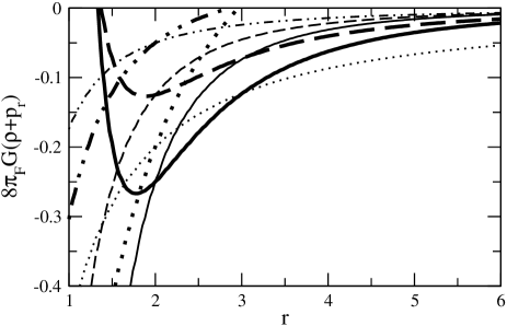
Figure 1: Plot showing $\rho+p_{r}<0$ for case 1. Here $n=0.0$, $0.2$, $0.5$ and $0.8$ represented by solid, dotted, dashed and chain curves, respectively. Thick curves represent $f(r)=r_{0}/r$ and thin curves represent f(r)=constant. We have assumed $r_{0}=2$ for the throat of the wormhole

Case 2: We choose the shape function, $b(r)=r_{0}+\rho_{0}r_{0}^{3}\ln(\frac{r_{0}}{r})$, where $r_{0}$ is the throat radius and $\rho_{0}$ is an arbitrary constant. However, for satisfying the flare out condition, one has to take $\rho_{0}$ as less than unity. We shall consider as above two cases with different redshift functions:

Subcase (2a): $f(r)=constant$
We find unknown parameters

$$\rho=\frac{(\lambda-1)r-\rho_{0}r_{0}^{3}}{8\pi_{F}r^{3}G},$$ (37)

$$p_{r}=\frac{(1-\lambda)r-[r_{0}+\rho_{0}r_{0}^{3}ln(\frac{r_{0}}{r})]}{8\pi_{F}r^{3}G},$$ (38)

$$p_{t}=\frac{r_{0}+\rho_{0}r_{0}^{3}[1+ln(\frac{r_{0}}{r})]}{16\pi_{F}r^{3}G},$$ (39)

$$\rho+p_{r}=-\frac{r_{0}+\rho_{0}r_{0}^{3}[1+ln(\frac{r_{0}}{r})]}{8\pi_{F}r^{3}G}.$$ (40)

Subcase (2b): $f(r)=\frac{r_{0}}{r}$
We obtain the unknown parameters as follows:

$$\rho=\frac{(\lambda-1)r-\rho_{0}r_{0}^{3}}{8\pi_{F}r^{3}G},$$ (41)

$$p_{r}=\frac{r(1-\lambda)-3r_{0}+\frac{2r_{0}^{2}}{r}+\rho_{0}r_{0}^{3}ln(\frac{r_{0}}{r})(\frac{2r_{0}}{r}-1)}{8\pi_{F}r^{3}G},$$ (42)

$$p_{t}=\frac{\frac{3r_{0}}{2}-\frac{r_{0}^{3}}{r^{2}}-\frac{r_{0}^{2}}{2r}+\rho_{0}r_{0}^{3}\left[\frac{1}{2}-\frac{r_{0}}{2r}+ln(\frac{r_{0}}{r})\left(\frac{1}{2}-\frac{3r_{0}}{2r}-\frac{r_{0}^{2}}{r^{2}}\right)\right]}{8\pi_{F}r^{3}G},$$ (43)

$$\rho+p_{r}=\frac{-3r_{0}+\frac{2r_{0}^{2}}{r}+\rho_{0}r_{0}^{3}[ln(\frac{r_{0}}{r})(\frac{2r_{0}}{r}-1)-1]}{8\pi_{F}r^{3}G}.$$ (44)

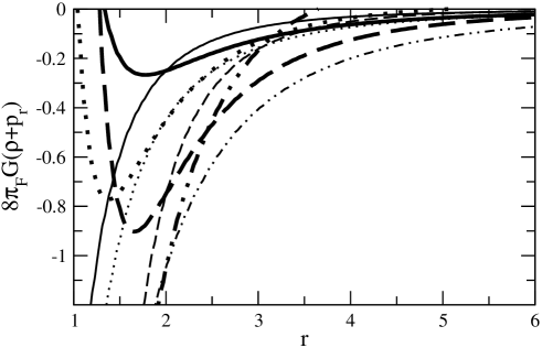
Figure 2: Plot showing $\rho+p_{r}<0$ for case 2. Here $\rho_{0}=0.0$, $0.2$, $0.5$ and $0.8$ represented by solid, dotted, dashed and chain curves, respectively. Thick curves represent $f(r)=r_{0}/r$ and thin curves represent f(r)=constant. We have assumed $r_{0}=2$ for the throat of the wormhole

Case 3: For the shape function, $b(r)=r_{0}+\gamma r_{0}(1-\frac{r_{0}}{r})$, where $r_{0}$ is the throat radius and $\gamma$ is an arbitrary constant, however, for satisfying the flare out condition, one has to take $\gamma$ as less than unity. We shall consider here also two cases with different redshift functions:

Subcase (3a): $f(r)=constant$
We obtain the unknown parameters

$$\rho=\frac{(\lambda-1)r+\gamma\frac{r_{0}^{2}}{r}}{8\pi_{F}r^{3}G},$$ (45)

$$p_{r}=\frac{(1-\lambda)r-r_{0}(1+\gamma)+\gamma\frac{r_{0}^{2}}{r}}{8\pi_{F}r^{3}G},$$ (46)

$$p_{t}=\frac{-2\gamma\frac{r_{0}^{2}}{r}+r_{0}(1+\gamma)}{16\pi_{F}r^{3}G},$$ (47)

$$\rho+p_{r}=\frac{2\gamma\frac{r_{0}^{2}}{r}-r_{0}(1+\gamma)}{8\pi_{F}r^{3}G}.$$ (48)

Subcase (3b): $f(r)=\frac{r_{0}}{r}$
We obtain the unknown parameters

$$\rho=\frac{(\lambda-1)r+\gamma\frac{r_{0}^{2}}{r}}{8\pi_{F}r^{3}G},$$ (49)

$$p_{r}=\frac{r(1-\lambda)-3r_{0}+\frac{2r_{0}^{2}}{r}+\gamma r_{0}(1-\frac{r_{0}}{r})(\frac{2r_{0}}{r}-1)}{8\pi_{F}r^{3}G},$$ (50)

$$p_{t}=\frac{\frac{3r_{0}}{2}-\frac{r_{0}^{3}}{r^{2}}-\frac{r_{0}^{2}}{2r}+\frac{\gamma r_{0}^{2}}{r}\left[\frac{r_{0}}{2r}-\frac{1}{2}\right]+\gamma r_{0}\left[1-\frac{r_{0}}{r}\right]\left[\frac{1}{2}-\frac{3r_{0}}{2r}-\frac{r_{0}^{2}}{r^{2}}\right]}{8\pi_{F}r^{3}G},$$ (51)

$$\rho+p_{r}=\frac{\gamma\frac{r_{0}^{2}}{r}-3r_{0}+\frac{2r_{0}^{2}}{r}+\gamma r_{0}(1-\frac{r_{0}}{r})(\frac{2r_{0}}{r}-1)}{8\pi_{F}r^{3}G}.$$ (52)

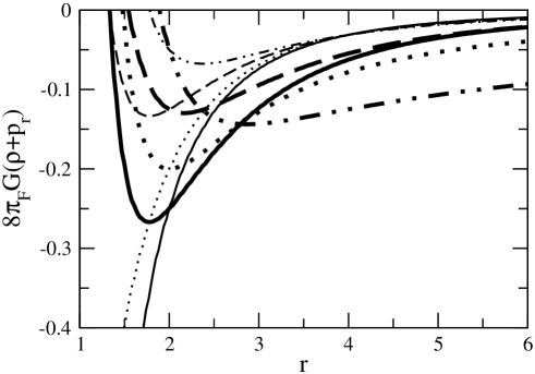
Figure 3: Plot showing $\rho+p_{r}<0$ for case 3. Here $\gamma=0.0$, $0.2$, $0.5$ and $0.8$ represented by solid, dotted, dashed and chain curves, respectively. Thick curves represent $f(r)=r_{0}/r$ and thin curves represent f(r)=constant. We have assumed $r_{0}=2$ for the throat of the wormhole

3.2 Specific energy density and redshift function

Case 4: For the specific energy density, $\rho=\rho_{0}(\frac{r_{0}}{r})^{\alpha}$, where $r_{0}$, $\rho_{0}$ and $\alpha$ are arbitrary constants, we shall consider two cases with different redshift functions:

Subcase (4a): $f(r)=constant$
Using the above choices of energy density and redshift function, we obtain the shape function $b(r)$ from field Eq. (26) as

$$b=c_{1}-\left[(\lambda-1)+\frac{8\pi_{F}r^{2}G\rho_{0}}{\alpha-3}\left(\frac{r_{0}}{r}\right)^{\alpha}\right]r,$$ (53)

where $c_{1}$ is an integration constant.

The radial and transverse pressures are obtained as

$$8\pi_{F}r^{2}Gp_{r}=\frac{8\pi_{F}r^{2}G\rho_{0}}{\alpha-3}\left(\frac{r_{0}}{r}\right)^{\alpha}-\frac{c_{1}}{r},$$ (54)

$$16\pi_{F}r^{2}Gp_{t}=\left[\frac{c_{1}}{r}-\left(\frac{\alpha-2}{\alpha-3}\right)8\pi_{F}r^{2}G\rho_{0}\left(\frac{r_{0}}{r}\right)^{\alpha}\right],$$ (55)

$$8\pi_{F}r^{2}G(\rho+p_{r})=\left(\frac{\alpha-2}{\alpha-3}\right)8\pi_{F}r^{2}G\rho_{0}\left(\frac{r_{0}}{r}\right)^{\alpha}-\frac{c_{1}}{r}.$$ (56)

Subcase (4b): $f(r)=\frac{r_{0}}{r}$
We obtain the unknown parameters

$$b=c_{1}-\left[(\lambda-1)+\frac{8\pi_{F}r^{2}G\rho_{0}}{\alpha-3}\left(\frac{r_{0}}{r}\right)^{\alpha}\right]r,$$ (57)

$$8\pi_{F}r^{2}Gp_{r}=\left[\frac{8\pi_{F}r^{2}G\rho_{0}}{\alpha-3}\left(\frac{r_{0}}{r}\right)^{\alpha}-\frac{c_{1}}{r}\right]\left[1-\frac{2r_{0}}{r}\right]-2\lambda\frac{r_{0}}{r},$$ (58)

$$8\pi_{F}r^{2}Gp_{t}=\left[\frac{8\pi_{F}r^{2}G\rho_{0}}{\alpha-3}\left(\frac{r_{0}}{r}\right)^{\alpha}-\frac{c_{1}}{r}\right]\left[\left(\frac{r_{0}}{r}\right)^{2}+\frac{r_{0}}{r}\right],$$ (59)

$$+\lambda\left[\left(\frac{r_{0}}{r}\right)^{2}+\frac{r_{0}}{r}\right]-\left[\frac{\alpha-2}{\alpha-3}8\pi_{F}r^{2}G\rho_{0}\left(\frac{r_{0}}{r}\right)^{\alpha}-\frac{c_{1}}{r}\right]\left[\frac{1}{2}-\frac{r_{0}}{2r}\right],$$ (60)

$$8\pi_{F}r^{2}G(\rho+p_{r})=\left[\frac{8\pi_{F}r^{2}G\rho_{0}}{\alpha-3}\left(\frac{r_{0}}{r}\right)^{\alpha}-\frac{c_{1}}{r}\right]\left[1-\frac{2r_{0}}{r}\right]-2\lambda\frac{r_{0}}{r}+8\pi r^{2}G\rho_{0}\left(\frac{r_{0}}{r}\right)^{\alpha}.$$ (61)

Note that $b(r)$ has the same form as the case $f=constant$. Therefore, we have same plots for $b(r)$, $b(r)-r$ and $b^{\prime}(r)$ when $f=constant$.

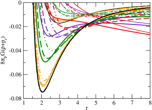
Figure 4: Plot showing $\rho+p_{r}<0$ for Case 4. Here, $\rho_{0}=0.001$, $0.01$, $0.05$, $0.10$ and $0.15$ are represented by black, orange, green, indigo and red colours, respectively. $\alpha$ is taken to be $0.0$, $1.0$ and $2.0$ are represented by solid, dashed and chain curves, respectively. Thick curves represent $f(r)=r_{0}/r$ and thin curves represent $f(r)=constant$. We have assumed $r_{0}=2$ and $c_{1}=1$

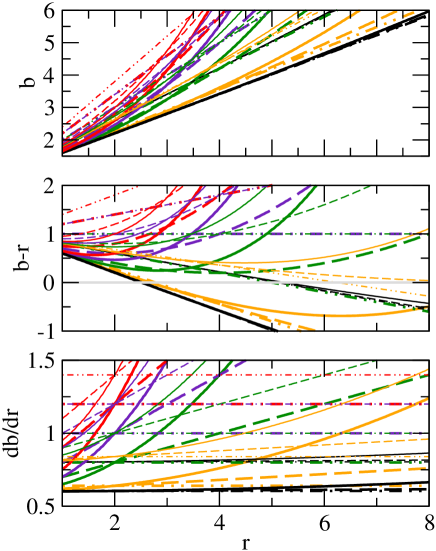
Figure 5: Plots (upper, middle and lower panels respectively) showing the behavior of the shape function, radii of the throat where $b-r$ cuts $r$ axis and nature of derivative of the shape function for Case 4. Here, $\rho_{0}=0.001$, $0.01$, $0.05$, $0.10$ and $0.15$ are represented by black, orange, green, indigo and red colours, respectively. $\alpha$ is taken to be $0.0$, $0.5$, $1.0$, $1.5$ and $2.0$, represented by solid, dotted, dashed, dot-dashed and chain curves, respectively. Thick curves represent $f(r)=r_{0}/r$ and thin curves represent $f(r)=constant$. We have assumed $r_{0}=2$ and $c_{1}=1$

Case 5: For the dark energy equation of state, $p_{r}=\omega\rho;~{}\omega<-1$, we shall consider as above two cases with different redshift functions:

Subcase (5a): $f(r)=$constant
Using the above choices of energy density and redshift function, we obtain the following parameters

$$b=(1-\lambda)r+r_{0}\left(\frac{r_{0}}{r}\right)^{(\frac{1}{\omega})},$$ (62)

$$8\pi_{F}r^{2}G\rho=-\frac{1}{\omega}\left(\frac{r_{0}}{r}\right)^{(\frac{1}{\omega}+1)},$$ (63)

$$8\pi_{F}r^{2}Gp_{r}=-\left(\frac{r_{0}}{r}\right)^{(\frac{1}{\omega}+1)},$$ (64)

$$8\pi_{F}r^{2}Gp_{t}=\frac{1}{2}\left(\frac{1}{\omega}+1\right)\left(\frac{r_{0}}{r}\right)^{(\frac{1}{\omega}+1)},$$ (65)

where $r_{0}^{(\frac{1}{\omega}+1)}$ is an integration constant.

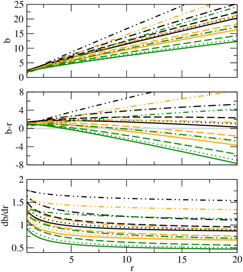
Figure 6: Plots showing the behavior of the shape function, radii of the throat where $b-r$ cuts $r$ axis and nature of derivative of the shape function for Case 5a. Here, $\lambda=0.2$, $0.4$ and $0.6$ represented by black, orange and green colors. Solid, dotted, dashed, dot-dashed and chain curves represent $\omega=-3.0$, $-2.5$, $-2.0$, $-1.5$, $-1.1$, respectively. We have assumed $r_{0}=2$ for the throat of the wormhole

Subcase (5b): $f(r)=\frac{r_{0}}{r}$
We obtain the unknown parameters as follows:

$$b=(1-\lambda)r+\left[\frac{4\lambda r_{0}^{2}}{\omega r}\right]\left[\left(-\frac{2r_{0}}{\omega r}\right)^{\left(\frac{1}{\omega}-1\right)}\exp\left(-\frac{2r_{0}}{\omega r}\right)\left\{\Gamma\left(1-\frac{1}{\omega}\right)-\Gamma\left(1-\frac{1}{\omega},-\frac{2r_{0}}{\omega r}\right)\right\}-\frac{\omega r}{2r_{0}}\right]+c_{3},$$ (66)

$$8\pi_{F}r^{2}G\omega\rho=(1-\lambda)+\left(\frac{2br_{0}}{r^{2}}-\frac{2r_{0}}{r}\right)-\frac{b}{r},$$ (67)

$$8\pi_{F}r^{2}Gp_{r}=(1-\lambda)+\left(\frac{2br_{0}}{r^{2}}-\frac{2r_{0}}{r}\right)-\frac{b}{r},$$ (68)

$$8\pi_{F}r^{2}Gp_{t}=\left[1-\frac{b}{r}\right]\left[\frac{r^{2}_{0}}{r^{2}}+\frac{r_{0}}{r}\right]-\left[(1-\lambda)\left(1+\frac{1}{\omega}\right)+\frac{1}{\omega}\left\{\frac{2br_{0}}{r^{2}}-\frac{2r_{0}}{r}\right\}-\left(1+\frac{1}{\omega}\right)\frac{b}{r}\right]$$

$$\times\left[\frac{1}{2}-\frac{r_{0}}{2r}\right],$$ (69)

where $c_{3}$ is an integration constant.

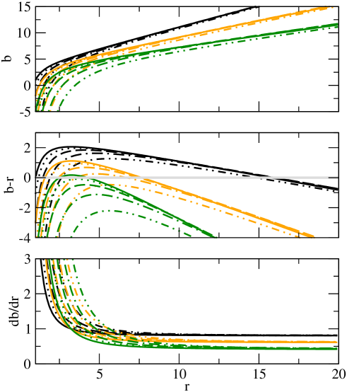
Figure 7: Plots showing the behavior of the shape function, radii of the throat where $b-r$ cuts $r$ axis and nature of derivative of the shape function for Case 5b. Here $\lambda=0.2$, $0.4$ and $0.6$, represented by black, orange and green colors. Solid, dotted, dashed, dot-dashed and chain curves represent $\omega=-3.0$, $-2.5$, $-2.0$, $-1.5$, $-1.1$, respectively. We have assumed $r_{0}=2$ and $c_{3}=3$

4 Discussion and Conclusion

Recent literature survey exhibits that the Finsler geometry has accumulated much attention due to its potentiality to explain various issues, specially as cosmic acceleration, which can be explained without invoking dark matter Chang2008 or dark energy Chang2009 . In the context of GR, the violation of NEC (often called exotic matter) is a basic ingredient of static traversable wormholes, although the violation of energy conditions is quite acceptable in certain quantum fields, among which the Casimir effect and Hawking evaporation are mentionable. The present work may be looked upon as a possible solutions to construct theoretically traversable wormholes in the context of Finsler geometry. In this context, we derived the Einstein gravitational field equations in the Riemannian spacetime with matter distribution as anisotropic in nature. We find out our solution in conventional way like the Morris-Thorne wormhole solution. We focus our attention mainly for discussing the violation of null energy condition (NEC) and the constraint on wormhole geometry, respectively.

In the present work we obtain exact solutions by imposing restricted choices of the redshift function, the shape function and/or specifying an equations of state. Some of the important features of the present investigation can be formulated as follows:

(i) In first three cases we consider the various choices for the form function, namely, $b(r)=r_{0}(\frac{r}{r_{0}})^{n}$, $b(r)=r_{0}+\rho_{0}r_{0}^{3}\ln(\frac{r_{0}}{r})$ and $b(r)=r_{0}+\gamma r_{0}(1-\frac{r_{0}}{r})$ and we have analyzed the solution by considering that the redshift function can either be constant, or have the functional relation of radial co-ordinate.

(ii) In the next two cases we have found out the shape functions for the specific form of energy density, namely, $\rho=\rho_{0}(\frac{r_{0}}{r})^{\alpha}$ and dark energy equation of state, $p_{r}=\omega\rho;~{}\omega<-1$.

After knowing all the metric potentials $f(r)$, $b(r)$ and stress-energy components $\rho$, $p_{r}$ and $p_{t}$, we examine whether the results indeed give wormhole structures. It is essentially required that to get a wormhole, the following properties must be satisfied:

1) The redshift function, $f(r)$, should remain finite everywhere to prevent an event horizon.

2) The shape function, $b(r)$, should obey the following flare-out conditions at the throat $r=r_{0}$ : $b(r_{0})=r_{0}$ and $b^{\prime}(r_{0})<1$, $r_{0}$ being the throat radius.

3) Another condition that needed to satisfy is $b(r)/r<1$ for $r>r_{0}$.

4) The NEC must be violated for traversable wormhole, i.e. $p_{r}+\rho<0$.

The first three conditions for the geometry of the spacetime and last one for the matter distribution that produces this spacetime.

We have, however, verified whether our models satisfy all the criteria to represent wormhole structure as follows:

In models 1-3, we have assumed that the spacetime produces wormholes and try to search for the matter distributions which produce these features. We have found out the components of the energy momentum tensors and Figs. 1-4 indicate the matter distributions violate the NEC. Note that violation of NEC is one of the important criteria to hold a wormhole open. Thus the first three models are physically valid. On the other hand, in models 4 and 5, we have found out the shape functions for the specific form of energy density and dark energy equation of state. For model 4, one can note that the shape function $b(r)$ assumes the same form for constant or specific redshift function. In Fig. 5, we have vividly depicted different characteristics of the shape function. We observe that existence of the throat depends on the choices of the parameters. The radius of the throat exists where $b(r)-r$ cuts $r$ axis. Also this figure indicates that flaring out condition is satisfied at the throat i.e. $b^{\prime}(r_{0})<1$. Thus in the model 4, the above four conditions are satisfied for development of wormholes structure.

We have also analyzed, in the model 5, different characteristics of the shape functions for different redshift functions in Figs. 6 and 7. These figures satisfy all the geometric criteria of the wormhole structure. In this case we have assumed dark energy equation of state, $p_{r}=\omega\rho;~{}\omega<-1$, and hence the NEC, $p_{r}+\rho<0$ is automatically satisfied. Thus, it is an overall observation that present models successfully describe the wormhole features under the background of the Finslerian spacetime.

Acknowledgments

FR, SR and AAU are thankful to IUCAA for providing Associateship under which a part the work was carried out. AB is also grateful to IUCAA for providing research facilities and hospitality. FR is thankful to DST, Govt. of India for providing financial support under PURSE programme. Finally we are grateful to the referee for several valuable comments and suggestions which have improved the manuscript substantially.

References

• (1) F. Rahaman, N. Paul, S.S. De, S. Ray, Md. A. Kayum Jafry, Eur. Phys. J. C 75, 564 (2015)
• (2) M.S. Morris, K.S. Thorne, Am. J. Phys. 56, 395 (1988)
• (3) M. Visser, Lorentzian Wormholes: From Einstein to Hawking (American Institute of Physics, New York, 1995)
• (4) D. Hochberg, M. Visser, Phys. Rev. D 56, 4745 (1997)
• (5) D. Ida, S.A. Hayward, Phys. Lett. A 260, 175 (1999)
• (6) M. Visser, S. Kar, N. Dadhich, Phys. Rev. Lett. 90, 201102 (2003)
• (7) C.J. Fewster, T.A. Roman, Phys. Rev. D 72, 044023 (2005)
• (8) P.K.F. Kuhfittig, Phys. Rev. D 73, 084014 (2006)
• (9) F. Rahaman et al., Phys. Lett. B 633, 161 (2006)
• (10) M. Jamil et al., Eur. Phys. J. C 67, 513 (2010)
• (11) D. Hochberg, M. Visser, Phys. Rev. D, 58, 044021 (1998)
• (12) S.A. Hayward, Int. J. Mod. Phys. D 8, 373 (1999)
• (13) J.P.S. Lemos, F.S.N. Lobo, S.Q. de Oliveira, Phys. Rev. D 68, 064004 (2003)
• (14) F. Rahaman, M. Kalam, M. Sarker, A. Ghosh, B. Raychaudhuri, Gen. Relativ. Gravit. 39, 145 (2007)
• (15) E. Teo, Phys. Rev. D, 58, 024014 (1998)
• (16) P.K.F. Kuhfittig, Phys. Rev. D 67, 064015 (2003)
• (17) D. Bao, S. S. Chern, Z. Shen, An Introduction to Riemann Finsler Geometry (Graduate Texts in Mathematics 200, Springer, New York, 2000)
• (18) E. Cartan, les Espaces de Finsler, Actualite Scientifiques et Industrielles, No. 79, Paris, Hermann (1934)
• (19) J.I. Horvath, Phys. Rev. 80, 901 (1950)
• (20) S. Vacaru, Phys. Lett. B 690, 224 (2010)
• (21) S. Vacaru, Int. J. Mod. Phys. D 21, 1250072 (2012)
• (22) M. Schreck, Eur. Phys. J. C 75, 187 (2015)
• (23) S. Vacaru, Nucl. Phys. B 434, 590 (1997)
• (24) S. Vacaru, J. Math. Phys. 37, 508 (1996)
• (25) S. Vacaru, Gen. Relativ. Gravit. 44, 1015 (2012)
• (26) P. Stavrinos, S. Vacaru, Class. Quant. Gravit. 30, 055012 (2013)
• (27) S. Rajpoot, S. Vacaru, Int. J. Geom. Meth. Mod. Phys. 12, 1550102 (2015)
• (28) Z. Chang, X. Li, Phys. Lett. B 668, 453 (2008)
• (29) Z. Chang, X. Li, Phys. Lett. B 676, 173 (2009)
• (30) Z. Chang et al., Mod. Phys. Lett. A 27, 1250058 (2012)
• (31) C. Pfeifer, M.N.R. Wohlfarth, Phys. Rev. D 85, 064009 (2012)
• (32) X. Li, Z. Chang, Phys. Rev. D 90, 064049 (2014)
• (33) X. Li, S. Wang, Z. Chang, Commun. Theor. Phys. 61, 781 (2014)
• (34) F.S.N. Lobo, Phys. Rev. D 73, 064028 (2006)
• (35) F. Rahaman, M. Jamil, R. Sharma, K. Chakraborty, Astrophys. Space Sci. 330, 249 (2010)
• (36) H. Akbar-Zadeh, Acad. Roy. Belg. Bull. Cl. Sci., 74, 281 (1988)
• (37) S. Carroll, “Space-time and Geometry”(monograph), Publ. Ad. Whes. (2014)