CP3-16-38

RM3-TH/16-8

Abstract

We propose a method to determine the trilinear Higgs self coupling that is alternative to the direct measurement of Higgs pair production total cross sections and differential distributions. The method relies on the effects that electroweak loops featuring an anomalous trilinear coupling would imprint on single Higgs production at the LHC. We first calculate these contributions to all the phenomenologically relevant Higgs production ($gg{\rm F}$, VBF, $WH$, $ZH$, $t\bar{t}H$) and decay ($\gamma\gamma$, $WW^{*}/ZZ^{*}\to 4f$, $b\bar{b}$, $\tau\tau$) modes at the LHC and then estimate the sensitivity to the trilinear coupling via a one-parameter fit to the single Higgs measurements at the LHC 8 TeV. We find that the bounds on the self coupling are already competitive with those from Higgs pair production and will be further improved in the current and next LHC runs.

1 Introduction

The discovery of a new scalar resonance with mass around 125 GeV at the Large Hadron Collider (LHC)Chatrchyan:2012xdj ; Aad:2012tfa opened a new era in high-energy particle physics. The study of the properties of this particle provides strong evidence that it is the Higgs boson of the Standard Model (SM), i.e., a scalar CP-even state whose couplings to the other known particles have a SM-like structure and strengths proportional to their masses. In particular, ATLAS and CMS performed both independent Khachatryan:2014jba ; Aad:2015gba and combined Khachatryan:2016vau studies on the Higgs couplings in the so-called $\kappa$-framework LHCHiggsCrossSectionWorkingGroup:2012nn ; Heinemeyer:2013tqa , where the predicted SM Higgs strengths $c_{i}$ are rescaled by overall factors $\kappa_{i}$. In the combined analysis based on 7 and 8 TeV data sets Khachatryan:2016vau the couplings with the vector bosons have been found to be compatible with those expected from the SM, i.e., $\kappa_{V}=1$ $(V=W,Z)$, within a $\sim 10\%$ uncertainty, while in the case of the heaviest SM fermions (the top, the bottom quarks and the $\tau$ lepton) the uncertainty is of order $\sim 15-20\%$. However, at this stage, additional relations among the different $\kappa_{i}$ that improve the sensitivity of experimental analyses are often assumed, yet lead to a loss of generality. The precision of the current measurements therefore still leaves room for Beyond-the-Standard-Model (BSM) scenarios involving modifications of the Higgs boson couplings to the vector bosons and fermions.

Besides the direct search of new particles, one of the main tasks of the second run of the LHC at $\sqrt{s}=13$ TeV centre-of-mass energy will be the precise determination of the properties and the interactions of the SM particles, in particular those of the Higgs boson, in order to constrain effects from New Physics (NP). The increase of the production cross sections together with a larger integrated luminosity, which is expected to reach 300 fb^-1 per experiment at the end of the Run II and up to 3000 fb^-1 in the case of the following High Luminosity (HL) option, will allow to probe the couplings of the Higgs boson with the other SM particles with much higher accuracy. In particular, present estimates CMS:2013xfa ; Peskin:2013xra , suggest that at the end of Run II the Higgs boson couplings to the vector bosons are expected to reach a $\sim 5\%$ precision with 300 fb^-1 luminosity, while the couplings to the heavy fermions could reach $\sim 10-15\%$ precision. Similar estimates for the end of the HL option indicate a reduction of these numbers by at least a factor $\sim 2$.

The study of the trilinear $(\lambda_{3})$ and quartic $(\lambda_{4})$ Higgs self couplings in the scalar potential

$$V(H)=\frac{m_{\scriptscriptstyle H}^{2}}{2}H^{2}+\lambda_{3}vH^{3}+\lambda_{4}H^{4}$$

is in a completely different situation. In the SM, the potential is fully determined by only two parameters, $v=(\sqrt{2}G_{\mu})^{-1/2}$ and the coefficient of the $(\Phi^{\dagger}\Phi)^{2}$ interaction $\lambda$, where $\Phi$ is the Higgs doublet field. Thus, the mass and the self couplings of the Higgs boson depend only on $\lambda$ and $v$ ($m_{\scriptscriptstyle H}^{2}=2\lambda v^{2},\lambda_{3}^{\rm SM}=\lambda,\lambda_{4}^{\rm SM}=\lambda/4$). On the contrary, in the case of extended scalar sectors or in presence of new dynamics at higher scales the trilinear and quartic couplings, $\lambda_{3}$ and $\lambda_{4}$, typically depend on additional parameters and their values can depart from the SM predictions Gupta:2013zza ; Efrati:2014uta .

At the Leading Order (LO) the Higgs decay widths and the cross sections of the main single Higgs production processes, i.e., gluon–gluon fusion ($gg{\rm F}$), vector-boson fusion (VBF), $W$ and $Z$ associated production ($WH$, $ZH$) and the production in association with a top-quark pair ($t\bar{t}H$), depend on the couplings of the Higgs boson to the other particles of the SM, yet they are insensitive to $\lambda_{3}$ and $\lambda_{4}$. Information on $\lambda_{3}$ can be directly obtained at LO only from final states featuring at least two Higgs bosons. However, the cross sections of these processes are much smaller than those of single Higgs production, due to the suppression induced by a heavier final state and an additional weak coupling. At $\sqrt{s}=13$ TeV the single Higgs gluon-gluon-fusion production cross section in the SM is around 50 pb Anastasiou:2016cez , while the double Higgs cross section is around 35 fb in the gluon-gluon-fusion channel deFlorian:2013jea ; Maltoni:2014eza ; Borowka:2016ehy and even smaller in other production mechanisms Baglio:2012np ; Frederix:2014hta .

A plethora of perspective studies performed at $\sqrt{s}=13$ TeV suggest that it should be possible to detect the production of a Higgs pair via $b\bar{b}\gamma\gamma$ Baur:2003gp ; Baglio:2012np ; Yao:2013ika ; Barger:2013jfa ; Azatov:2015oxa ; Lu:2015jza , $b\bar{b}\tau\tau$ Dolan:2012rv ; Baglio:2012np , $b\bar{b}W^{+}W^{-}$ Papaefstathiou:2012qe and $b\bar{b}b\bar{b}$ deLima:2014dta ; Wardrope:2014kya ; Behr:2015oqq final states, and also via signatures emerging from $t\bar{t}HH$ Englert:2014uqa ; Liu:2014rva and $HVV$ Cao:2015oxx production channels. However, the ultimate precision that could be achieved on the determination of $\lambda_{3}$ is much less clear. Even with an integrated luminosity of 3000 fb^-1, experimental analyses suggest that it will be possible to exclude at the LHC only values in the range $\lambda_{3}<-1.3~{}\lambda_{3}^{\rm SM}$ and $\lambda_{3}>8.7~{}\lambda_{3}^{\rm SM}$ via the $b\bar{b}\gamma\gamma$ signatures ATL-PHYS-PUB-2014-019 or $\lambda_{3}<-4~{}\lambda_{3}^{\rm SM}$ and $\lambda_{3}>12~{}\lambda_{3}^{\rm SM}$ even including also $b\bar{b}\tau\tau$ signatures ATL-PHYS-PUB-2015-046 , i.e., a much more pessimistic perspective than the results reported in the phenomenological explorations. The current experimental bounds on non-resonant Higgs pair production cross sections as obtained at 8 TeV are rather weak. ATLAS has been able to exclude only a signal up to 70 times larger than the SM one Aad:2015xja ; Aad:2015uka , which can be roughly translated to the $\lambda_{3}<-12~{}\lambda_{3}^{\rm SM}$ and $\lambda_{3}>17~{}\lambda_{3}^{\rm SM}$ exclusion limits, while CMS puts a 95$\%$ C.L.  exclusion limit on $\lambda_{3}<-17.5~{}\lambda_{3}^{\rm SM}$ and $\lambda_{3}>22.5~{}\lambda_{3}^{\rm SM}$ assuming changes only in the trilinear Higgs boson coupling, with all other parameters fixed to their SM values Khachatryan:2016sey . Thus, additional strategies in the determination of the trilinear Higgs self coupling $\lambda_{3}$ that are alternative and complementary to the constrains from Higgs pair production would be certainly helpful. Finally, the perspectives of determining the quartic Higgs self coupling $\lambda_{4}$ via measurements in triple Higgs production seems quite bleak at the LHCPlehn:2005nk ; Binoth:2006ym , due to the smallness of the corresponding cross section Maltoni:2014eza .

In this work we explore the possibility of constraining the trilinear Higgs self coupling with a different approach, namely, via precise measurements of processes featuring single Higgs production and decay at the LHC. Indeed, although single Higgs production does not depend on $\lambda_{3}$ at LO or at higher orders in QCD, it does depend on $\lambda_{3}$ via weak loops, namely at Next-to-Leading (NLO) in the electroweak (EW) interactions. We therefore extract the $\lambda_{3}$-dependent part from the NLO EW corrections to all phenomenologically relevant single Higgs production cross sections ($gg{\rm F}$, VBF, $WH$, $ZH$, $t\bar{t}H$) and branching ratios, ($H\rightarrow\gamma\gamma$, $H\rightarrow ZZ^{*},WW^{*}\rightarrow 4f$, $H\rightarrow f\bar{f}$, $H\rightarrow gg$). By varying the value of $\lambda_{3}$, we evaluate the impact of an anomalous trilinear Higgs self coupling on the predictions for the aforementioned cross sections and decay widths. We obtain a distinctive pattern of deformations of the SM predictions for the rates ($\sigma(i)\cdot{\rm BR}(f)$), which can be compared to the experimental data. A similar investigation, specific to $ZH$ production at an $e^{+}e^{-}$ collider, was presented in Ref.McCullough:2013rea .

Our approach builds on the assumption that NP couples to the SM via the Higgs potential and dominantly affects only the Higgs self couplings. In other words, the lowest-order Higgs couplings to the other fields of the SM (and in particular to the top quark and vector bosons) are still given by the SM prescriptions or, equivalently, modifications to these couplings are so small that do not swamp the NLO effects we are considering. While this assumption needs always to be kept in mind, we stress that all the current experimental limits or estimates of limits on $\lambda_{3}$ obtained from Higgs pair production implicitly rely on it, too. In particular, the top-quark-Higgs coupling is assumed to be the one of the SM. Perspectives on measurements of $\lambda_{3}$ via Higgs pair production relaxing this assumption have been studied at the phenomenological level, e.g., in Refs. Goertz:2014qta ; Azatov:2015oxa leading, in general, to much weaker bounds. Within the assumption that NP modifies only $\lambda_{3}$, we investigate the reach of our approach in the determination of $\lambda_{3}$ by considering the current 8 TeV Higgs data Khachatryan:2016vau and the expected performances of the forthcoming runs of the LHC CMS:2013xfa ; Peskin:2013xra . We demonstrate the potential of single Higgs production channels in setting bounds on $\lambda_{3}$ that are competitive and complementary to those achievable via the searches for double Higgs production.

The paper is organised as follows. In Section 2 we present the theoretical framework and discuss the $\lambda_{3}$-dependent part of the NLO EW corrections to the single Higgs processes. In the following section we present the calculation of such contributions to the various observables. Section 4 is devoted to study the impact of the $\lambda_{3}$-dependent contribution in the single Higgs production and decay modes at the LHC, while in the following section we discuss the constraints on $\lambda_{3}$ that can be obtained from the current data and also from future measurements. In the last section we summarise and draw our conclusions.

2 $\lambda_{3}$-dependent contributions in single Higgs processes

As basic assumption, we consider a BSM scenario where the only (or dominant) modification of the SM Lagrangian at low energy appears in the scalar potential. In other words, we assume that the only relevant effect induced at the weak scale by unknown NP at a high scale is a modification of the self couplings of the 125 GeV boson. In particular, we concentrate on the trilinear self-coupling of the Higgs boson, making the assumption that modifications of $\lambda_{4}$ and of possible other self-couplings in the potential lead to much smaller effects and that the strength of tree-level interactions of the Higgs field with the vector bosons and with the fermions is not (or very weakly) modified with respect to the SM case. We therefore simply parametrise the effect of NP at the weak scale via a single parameter $\kappa_{\lambda}$, i.e., the rescaling of the SM trilinear coupling, $\lambda_{3}^{\rm SM}$. Thereby, the $H^{3}$ interaction in the potential, where $H$ is the physical Higgs field, is given by

$$V_{H^{3}}=\lambda_{3}\,v\,H^{3}\equiv\kappa_{\lambda}\lambda_{3}^{\rm SM}\,v\,H^{3},\qquad\lambda_{3}^{\rm SM}=\frac{G_{\mu}}{\sqrt{2}}m_{\scriptscriptstyle H}^{2}\,,$$ (1)

with the vacuum expectation value, $v$, related to the Fermi constant at the tree-level by $v=(\sqrt{2}\,G_{\mu})^{-1/2}$.

As we will discuss and quantify in more detail in the following, the “deformation" of the Higgs trilinear coupling induces modifications of the Higgs couplings to fermions and to vector bosons at one loop. However, since such loop-induced $\lambda_{3}$-dependent contributions are energy- and observable-dependent, the resulting modifications cannot be parameterised via a rescaling of the tree-level couplings of the single Higgs production and decay processes considered. Thus, it is important to keep in mind that the effects discussed in this work cannot be correctly captured by the standard $\kappa$-framework LHCHiggsCrossSectionWorkingGroup:2012nn ; Heinemeyer:2013tqa .

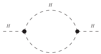
Figure 1: One-loop $\lambda_{3}$-dependent diagram in the Higgs self-energy.

Let us now start by classifying the $\lambda_{3}$-dependent contributions that come from the $\mathcal{O}(\alpha)$ corrections to single Higgs production and decay processes. These contributions can be divided into two categories: a universal part, i.e., common to all processes, quadratically dependent on $\lambda_{3}$ and a process-dependent part linearly proportional to $\lambda_{3}$.

The universal $\mathcal{O}({\lambda_{3}}^{2})$ corrections originate from the diagram in the wave function renormalisation constant of the external Higgs field, see Fig. 1. This contribution represents a renormalisation factor common to all the vertices where the Higgs couples to vector bosons or fermions. Thus, for on-shell Higgs boson production and decay, it induces the same effect for all processes, without any dependence on the kinematics. Denoting as $\mathcal{M}$ a generic amplitude for single Higgs production or a Higgs decay width, the correction to $\mathcal{M}$ induced by the $\lambda_{3}$-dependent diagram of Fig. 1 can be written as

$$\left(\delta\mathcal{M}\right)_{Z_{H}}=\left(\sqrt{Z_{H}}-1\right)\mathcal{M}^{0},~{}~{}~{}~{}~{}~{}~{}~{}Z_{H}=\frac{1}{1-\kappa_{\lambda}^{2}\,\delta Z_{H}}\,,$$ (2)

where $\mathcal{M}^{0}$ is the lowest-order amplitude and

$$\delta Z_{H}=-\frac{9}{16}\,\frac{G_{\mu}\,m_{\scriptscriptstyle H}^{2}}{\sqrt{2}\,\pi^{2}}\left(\frac{2\pi}{3\sqrt{3}}-1\right)\,.$$ (3)

In order to extend the range of convergence of the perturbative expansion to large values of $\kappa_{\lambda}$, the one-loop contribution in $Z_{H}$ has been resummed. In so doing, terms of $\mathcal{O}((\kappa_{\lambda}^{2}\alpha)^{n})$ which are expected to be the dominant higher-order corrections at large $\kappa_{\lambda}$ are correctly accounted for.

In addition to the ${\lambda_{3}}^{2}$ universal term above, amplitudes depend linearly on $\lambda_{3}$ differently for each process and kinematics. Let $\mathcal{M}^{0}$ be the Born amplitude corresponding to a given process (production or decay). At the level of cross section or decay width, the linear dependence on $\lambda_{3}$ originates from the interference of the Born amplitude $\mathcal{M}^{0}$ and the virtual EW amplitude $\mathcal{M}^{1}$, besides the wave function renormalisation constant. The amplitude $\mathcal{M}^{1}$ involves one-loop diagrams when the process at LO is described by tree-level diagrams, like, e.g., vector boson fusion production, while it involves two-loop diagrams when the LO contribution is given by one-loop diagrams, like, e.g., gluon-gluon-fusion production. The $\lambda_{3}$-linearly-dependent contributions in $\mathcal{M}^{1}$, which we denote as $\mathcal{M}^{1}_{\lambda_{3}}$, can be obtained for any process by evaluating in the SM the diagrams that contain one trilinear Higgs coupling ($\mathcal{M}^{1}_{\lambda_{3}^{\rm SM}}$) and then rescaling them by a factor $\kappa_{\lambda}$. In order to correctly identify $\mathcal{M}^{1}_{\lambda_{3}^{\rm SM}}$ (the contributions related to the $H^{3}$ interaction) in the $\mathcal{M}^{1}$ amplitude in the SM, it is convenient to choose a specific gauge, namely the unitary gauge. In a renormalisable $R_{\xi}$ gauge, $\lambda_{3}^{\rm SM}$-dependent diagrams are due not only to the interaction among three physical Higgs fields but also to the interaction among one physical Higgs and two unphysical scalars, making the identification less straightforward.

Once all the contributions from $\mathcal{M}^{1}_{\lambda_{3}}$ and $Z_{H}$ are taken into account, denoting as $\Sigma$ a generic cross section for single Higgs production or a Higgs decay width, the corrections induced by an anomalous trilinear coupling modify the LO prediction ($\Sigma_{\rm{LO}}$) according to

$$\Sigma_{\rm{NLO}}=Z_{H}\,\Sigma_{\rm{LO}}\left(1+\kappa_{\lambda}C_{1}\right)\,,$$ (4)

where the coefficient $C_{1}$, which originates from $\mathcal{M}^{1}_{\lambda_{3}^{\rm SM}}$, depends on the process and the kinematical observable considered, while $Z_{H}$ is universal, see Eq. (2). Here and in the following the LO contribution is understood as including QCD corrections so that the labels LO and NLO refer to EW corrections. We remind that among all terms contributing to the complete EW corrections we consider only the part relevant for our discussion, i.e., the one related to the Higgs trilinear interaction. The $\Sigma_{\rm{NLO}}$ in the SM can be obtained from Eq. (4) setting $\kappa_{\lambda}=1$ and expanding the $Z_{H}$ factor, or

$$\Sigma^{\rm SM}_{\rm{NLO}}=\Sigma_{\rm{LO}}\left(1+C_{1}+\delta Z_{H}\right)\,.$$ (5)

Thus, the relative corrections induced by an anomalous trilinear Higgs self-coupling can be expressed as

$$\delta\Sigma_{\lambda_{3}}\equiv\frac{\Sigma_{\rm{NLO}}-\Sigma^{\rm SM}_{\rm{NLO}}}{\Sigma_{\rm{LO}}}=Z_{H}-(1+\delta Z_{H})+(Z_{H}\kappa_{\lambda}-1)C_{1}\,,$$ (6)

which, neglecting $\mathcal{O}(\kappa_{\lambda}^{3}\,\alpha^{2})$ terms in the r.h.s, can be compactly written as

$$\delta\Sigma_{\lambda_{3}}=(\kappa_{\lambda}-1)C_{1}+(\kappa_{\lambda}^{2}-1)C_{2}\,,$$ (7)

with

$$C_{2}=\frac{\delta Z_{H}}{(1-\kappa_{\lambda}^{2}\delta Z_{H})}~{}.$$ (8)

Before describing the method and results of the calculation of the $C_{1}$ coefficients, we scrutinise the theoretical robustness of Eq. $\eqref{corr}$ and its range of validity. Our aim is to employ Eq. $\eqref{corr}$ to evaluate the LHC sensitivity on $\lambda_{3}$ without making “a priori” any assumptions on the value of the parameter $\kappa_{\lambda}$. We will, however, demand as a consistency constraint that, for large values of $\kappa_{\lambda}$, $\lambda_{3}$-dependent terms from $\mathcal{O}(\alpha^{j})$ corrections with $j>1$ do not overwhelm the effects from the $C_{i}$ coefficients. In order to take into account all the $\mathcal{O}((\kappa_{\lambda}^{2}\alpha)^{n})$ contributions and perform a resummation of the $\kappa_{\lambda}^{2}\,\delta Z_{H}$ terms in $Z_{H}$ we need to impose that $\kappa_{\lambda}^{2}\,\delta Z_{H}\lesssim 1$, i.e., $|\kappa_{\lambda}|\lesssim 25$. The corresponding parametric uncertainty in $\Sigma_{\rm{NLO}}$ is therefore given by $\mathcal{O}((\kappa_{\lambda}^{3}\alpha^{2}))$ terms that can be sizeable for large values of $\kappa_{\lambda}$. The size of such missing terms can be estimated by calculating the difference between $\delta\Sigma_{\lambda_{3}}$ computed using Eq. (6) and Eq. (7), or equivalently $\delta(\Sigma_{\rm{NLO}}/\Sigma_{\rm{LO}})\simeq\kappa_{\lambda}^{3}C_{1}\delta Z_{H}$. Requiring this uncertainty to be $\lesssim 10\%$ and assuming as an order of magnitude of the two-loop contribution $C_{1}\delta Z_{H}\sim 10^{-5}$, we find $|\kappa_{\lambda}|\lesssim 20$, which we take as the range of validity of our perturbative calculation.

At variance with the SM, where the Higgs self coupling and the Higgs mass are related, in our setup they are two independent parameters. This in general spoils the renormalisability of the model and makes its parameters sensitive to the UV scales. However, one knows a priori that the $\lambda_{3}$–dependent $\mathcal{O}(\alpha)$ corrections to $\Sigma$ in Eq. (6) are finite. The reason is twofold:

i) the LO result does not depend on $\lambda_{3}$ and therefore no renormalisation of $\lambda_{3}$ at NLO is either needed nor possible.

ii) All the counterterms needed at NLO do not contain divergent contributions proportional to the trilinear coupling.

This last point can be understood as follows: the only counterterm that contains divergent contributions proportional to $\lambda_{3}$ is the Higgs mass counterterm. However, the $m_{\scriptscriptstyle H}$ dependence in $\Sigma_{\rm LO}$ is all of kinematical origin. Therefore, when the NLO corrections are calculated, no renormalisation of $m_{\scriptscriptstyle H}$ is needed.

The arguments above are sufficient for all the processes except for $H\to\gamma\gamma$, which deserves a dedicated discussion. In a $R_{\xi}$ gauge the LO dependence of $\Gamma(H\to\gamma\gamma)$ upon $m_{\scriptscriptstyle H}$ is not purely kinematical, but it also comes from diagrams containing unphysical charged scalars. Therefore one expects that in these gauges at NLO there is no clear way to disentangle the contributions that can be assigned as due to a trilinear coupling from the ones related to the kinematical parameter $m_{\scriptscriptstyle H}$. In order to overcome this difficulty, as we already said, we employed the unitary gauge. In this gauge all the LO $m_{\scriptscriptstyle H}$ dependence of $\Gamma(H\to\gamma\gamma)$ is kinematical, similarly to all the other observables we considered, and the argument discussed above about the finiteness of the NLO $\lambda_{3}$–dependent corrections applies.

In general, an anomalous coupling $c_{i}$ is a free parameter that does not satisfy the SM relations that can be crucial for the renormalisability of the model. In the calculation of radiative corrections, the substitution of an electroweak coupling with an anomalous one, $c_{i}^{\rm SM}\rightarrow c_{i}\equiv\kappa_{i}c_{i}^{\rm SM}$ gives a finite result in two cases. First, when the renormalisation of $c_{i}$ does not involve EW corrections. Second, when the renormalisation of the other regular couplings $c_{j}$ involves $c_{i}$ via EW corrections, but $c_{i}$ itself is not renormalised. The first case corresponds to what happens in the context of the $\kappa-$formalism where couplings are rescaled by overall factors. It also applies to many phenomenological and experimental studies on the dependence of double Higgs production cross sections on $\lambda_{3}$ as done, e.g, in Baglio:2012np or in the experimental studies ATL-PHYS-PUB-2014-019 ; ATL-PHYS-PUB-2015-046 . In this case only QCD higher-order corrections can be consistently included. The second case corresponds to the study presented here: $\Sigma$ at LO does not depend on $\lambda_{3}$ and the NLO EW corrections, which do depend on $\lambda_{3}$, are finite because do not involve the renormalisation of $\lambda_{3}$. At this point, it is worth stressing that studies analogous in spirit and philosophy to ours have been performed for the case of the top-Higgs Yukawa coupling $y_{t}$, where, by looking at the dependence of NLO EW corrections, bounds on anomalous $y_{t}\equiv\kappa_{t}y_{t}^{\rm SM}$ can be set via the analysis of top-quark pair production measurements Kuhn:2013zoa ; Beneke:2015lwa .

It should be said that, while the $\mathcal{O}(\alpha_{s}^{i}\alpha)$ corrections to the physical observables $\Sigma$ due to an anomalous trilinear Higgs coupling are finite, and therefore they do not provide us with direct information about the scale $\Lambda$ of NP, one expects that the $\mathcal{O}(\alpha_{s}^{i}\alpha^{j})$ corrections with $j>1$ will instead show at least a logarithmic sensitivity to $\Lambda$. For our analysis to be trustworthy, one has to therefore make the further assumption that the scale $\Lambda$ is not too far from the EW scale, such that potentially large logarithmic corrections that would spoil the perturbativity of our analysis are not there.

In summary, we have argued that loop-induced dependence of single Higgs processes on $\lambda_{3}$ can be seen in the same spirit as, for example, the dependence of Higgs pair production cross sections on $\lambda_{3}$ or the general fits of the anomalous Higgs couplings at the LHC in the $\kappa$-framework. The variable $\kappa_{\lambda}$ in Eq. (6) is a parameter that can be directly probed at the experimental level, looking for discrepancies from SM predictions. The value of $\kappa_{\lambda}$ is a priori unconstrained, besides the limits imposed by perturbativity; constraints on its value can be set via experimental data. Clearly, if an UV-completed BSM model is specified or an EFT approach is used then different range of validity should be set on the parameter $\kappa_{\lambda}$.

Finally, let us stress that our investigation probes a larger range of $\kappa_{\lambda}$ with respect to an Effective-Field-Theory approach based on the addition of the dimension six operator $(\Phi^{\dagger}\Phi)^{3}$, as proposed for instance in Ref. Gorbahn:2016uoy . In this case the requirement that the potential is bounded from below and $v$ being the absolute minimum sets the constraints $1<\kappa_{\lambda}<3$ as shown in Appendix A.

3 Computation of the $C_{1}$ coefficients

At variance with the $C_{2}$ coefficient, which is universal, the $C_{1}$ coefficients are process- and kinematic-dependent and therefore need separate calculations. In this work we focus on the main production and decay channels:

• $\sigma_{gg{\rm F}}$, the gluon-gluon-fusion cross section;

• $\sigma_{\text{VBF}}$, the VBF cross section;

• $\sigma_{WH}$, $\sigma_{ZH}$, the cross section for associate production with $W$ and $Z$ bosons;

• $\sigma_{t\bar{t}H}$, the cross section for $t\bar{t}H$ production;

• $\Gamma_{\gamma\gamma}$, the decay width into photons;

• $\Gamma_{ZZ}$ and $\Gamma_{WW}$, the decay widths into $ZZ^{*}$ and $WW^{*}$ subsequently decaying into fermions;

• $\Gamma_{f\bar{f}}$, the decay width into fermions;

• $\Gamma_{gg}$, the decay width into gluons.

For each observable, the corresponding $C_{1}$ coefficient is identified as the contribution linearly proportional to $\lambda_{3}^{\rm SM}$ in the NLO EW corrections and normalised to the LO result as evaluated in the SM.

For any given single Higgs process, in principle $C_{1}$ could be evaluated directly at the level of matrix element in a fully differential way, i.e., point by point in phase space

$$C_{1}(\{p_{n}\})=\frac{2\Re(\mathcal{M}^{0*}\mathcal{M}^{1}_{\lambda_{3}^{\rm SM}})}{|\mathcal{M}^{0}|^{2}}\,,$$ (9)

where we have explicitly shown in parentheses the dependence on the external momenta $\{p_{n}\}$ in the Born configuration and understood the sum/average over helicities and colour states. By integrating over the phase space the differential ratio in Eq. (9) one would achieve the maximal discriminating power between the $\kappa_{\lambda}=1$ hypothesis and the $\kappa_{\lambda}\neq 1$ ones. However, as first step, it is both useful and convenient to work at the more inclusive level and directly compute $C_{1}$ for cross sections or decay rates integrated over the entire phase space or a portion of it.

For example, in the case of the decays, in this work we limit the discussion to total rates and define $C_{1}^{\Gamma}$ as

$$C_{1}^{\Gamma}=\frac{\int d\Phi~{}2\Re\left(\mathcal{M}^{0*}\mathcal{M}^{1}_{\lambda_{3}^{\rm SM}}\right)}{\int d\Phi~{}|\mathcal{M}^{0}|^{2}}\,,$$ (10)

where the integration in $d\Phi$ is over the phase space of the final-state particles.

The computation of (total or differential) hadronic cross sections is more involved than that of the decay widths, because hadronic cross sections receive contributions from different partonic process, which have to be convoluted with the corresponding parton luminosities and in principle can have different $C_{1}$ terms at the level of matrix elements. For production cross section, $C_{1}^{\sigma}$ reads

$$C_{1}^{\sigma}=\frac{\sum_{i,j}\int dx_{1}dx_{2}f_{i}(x_{1})f_{j}(x_{2})\,2\Re\left(\mathcal{M}_{ij}^{0*}\mathcal{M}^{1}_{\lambda_{3}^{\rm SM},ij}\right)d\Phi}{\sum_{i,j}\int dx_{1}dx_{2}f_{i}(x_{1})f_{j}(x_{2})\,|\mathcal{M}_{ij}^{0}|^{2}d\Phi}\,,$$ (11)

where the sum is over all the possible $i,j$ partonic initial states of the process, which are convoluted with the corresponding parton distribution functions.

A few comments on the $C_{1}$ for the various observables considered here are in order before showing the results. Assuming that all the fermions but the top quark are massless, the $C_{1}^{\Gamma}$ for $H\rightarrow ZZ^{*}\rightarrow 4f$ does not depend on the fermions in the final state. The same applies to $H\rightarrow WW^{*}\rightarrow 4f$. In the case of hadronic production, different partonic processes can have different $C_{1}$’s at the level of matrix elements. One example is $t\bar{t}H$ production, which receives contributions from $q\bar{q}\rightarrow t\bar{t}H$ and $gg\rightarrow t\bar{t}H$. Another is VBF, where both $W$-boson-fusion and $Z$-boson-fusion contribute. Moreover, each subprocess contributes in proportion to the parton distribution weights.

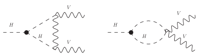
Figure 2: Structure of the $\lambda_{3}^{\rm SM}$-dependent part in $\mathcal{M}^{1}_{\lambda_{3}^{\rm SM}}$ for processes involving massive vector bosons in the final or in the intermediate states (VBF, $HV$ and $H\rightarrow VV^{*}\rightarrow 4f$).

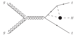
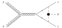
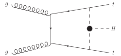
Figure 3: Sample of $\lambda_{3}^{\rm SM}$-dependent diagrams in $t\bar{t}H$ production.

In order to evaluate the $C_{1}$ coefficients of the various processes, we generated the relevant amplitudes using the Mathematica package FeynArts Hahn:2000kx . For all the cases involving only one-loop amplitudes, we computed the cross sections and decay rates with the help of FormCalc interfaced to LoopTools Hahn:1998yk and we checked the partonic cross sections at specific points in the phase space with FeynCalc Mertig:1990an ; Shtabovenko:2016sxi . In processes involving massive vector bosons in the final or in the intermediate states (VBF, $HV$ and $H\rightarrow VV^{*}\rightarrow 4f$), the $\lambda_{3}$-dependent parts in $\mathcal{M}^{1}_{\lambda_{3}^{\rm SM}}$ have a common structure, see Fig. 2. In the case of the $t\bar{t}H$ production the sensitivity to $\lambda_{3}$ comes from the one-loop corrections to the $t\bar{t}H$ vertex and from one-loop box and pentagon diagrams. A sample of diagrams containing these $\lambda_{3}$-dependent contributions is shown in Fig. 3.

The presence of not only triangles but also boxes and pentagons in the case of $t\bar{t}H$ production provides an intuitive explanation of why the $\lambda_{3}$ contributions cannot be captured by a local rescaling of the type that a standard $\kappa$-framework would assume for the top-Higgs coupling. Similarly, not all the contributions given by the corrections to the $HVV$ vertex can be described by a scalar modification of its SM value via a $\kappa_{V}$ factor, due to the different Lorentz structure at one loop and at the tree level.

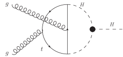
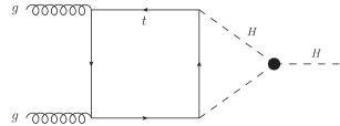
Figure 4: Diagrams contributing to the $C_{1}$ coefficient in the gluon-gluon-fusion Higgs production. The one on the right has a multiplicity factor 2.

The computation of $\sigma(gg\rightarrow H)$, the related $\Gamma(H\to gg)$, and of $\Gamma(H\rightarrow\gamma\gamma)$ is much more challenging and deserves a more detailed discussion. These observables receive the first non-zero contributions from one-loop diagrams, which do not feature $\lambda_{3}$, so that the computation of $C_{1}$ requires the evaluation of two-loop diagrams.

The two-loop EW corrections to $\sigma(gg\rightarrow H)$ in the SM were obtained in Refs.Aglietti:2004nj ; Degrassi:2004mx ; Actis:2008ug . In our computation of the $C_{1}$ coefficient we followed the approach of Ref. Degrassi:2004mx where the corrections have been computed via a Taylor expansion in the parameters $q^{2}/(4m_{t}^{2}),\>q^{2}/(4m_{\scriptscriptstyle H}^{2})$ where $q^{2}$ is the virtuality of the external Higgs momentum, to be set to $m_{\scriptscriptstyle H}^{2}$ at the end of the computation. However, at variance with Ref.Degrassi:2004mx , we computed the diagrams contributing to $C_{1}$, see Fig. 4, via an asymptotic expansion in the large top mass up to and including ${\cal O}(m_{\scriptscriptstyle H}^{6}/m_{t}^{6})$ terms. The two expansions are equivalent up to the first threshold encountered in the diagrams that defines the range of validity of the Taylor expansion. In our case, the first threshold in the diagrams of Fig. 4 occurs at $q^{2}=4\,m_{\scriptscriptstyle H}^{2}$ and both expansions are valid for $m_{\scriptscriptstyle H}\simeq 125$ GeV. The asymptotic expansion was performed following the strategy described in Ref.Degrassi:2010eu and the result for $C_{1}$ is presented in Appendix B. We checked our asymptotic expansion against the corresponding expression obtained by the Taylor expansion finding, as expected, very good numerical agreement.

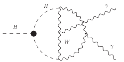
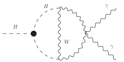
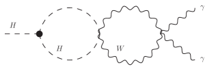
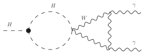
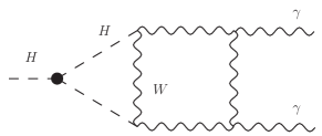
Figure 5: Diagrams contributing to the $C_{1}$ coefficient in $\Gamma(H\to\gamma\gamma)$. The diagrams in the second row have multiplicity 2.

The computation of the EW corrections to the partial decay width of a Higgs boson into two photons in the SM was performed in a $R_{\xi}$ gauge in Refs.Degrassi:2005mc ; Actis:2008ts . As mentioned above, the identification of the contributions to the $C_{1}$ coefficient is straightforward in the unitary gauge. In this gauge, neither unphysical scalars nor ghosts are present and the propagator of the massive vector bosons is $i(-g_{\mu\nu}+k_{\mu}k_{\nu}/M_{V}^{2})/(k^{2}-M_{V}^{2}+i\epsilon)$. The unitary gauge is a very special gauge. It can be defined as the limit when the gauge parameter $\xi$ is sent to infinity of a $R_{\xi}$ gauge. When a calculation is performed in the unitary gauge, one is actually interchanging the order of the operations limit $\xi\to\infty$ with the integration, i.e., the limit $\xi\to\infty$ is performed first and then one does the integration while the correct order is the opposite. Because some of the vertices that arise from the gauge-fixing function contain a $\xi$ factor, this exchange is not always an allowed operation and in order to check the correctness of our approach we recomputed the full two-loop EW corrections to $\Gamma(H\to\gamma\gamma)$ in the unitary gauge. The corrections were computed as in Ref.Degrassi:2005mc via a Taylor expansion in the parameters $q^{2}/(4m_{t}^{2}),\>q^{2}/(4m_{\scriptscriptstyle W}^{2}),\>q^{2}/(4m_{\scriptscriptstyle H}^{2})$ up to and including ${\cal O}(q^{6}/m^{6})$ terms finding perfect agreement with the result of Ref.Degrassi:2005mc .

Once we verified that in the SM the calculation in the unitary gauge is equivalent to the one in a $R_{\xi}$ gauge, the coefficient $C_{1}$ is obtained evaluating the diagrams in the unitary gauge that contain one trilinear Higgs interaction. The latter amounts to add to the contribution of the diagrams in Fig. 4, with the gluons replaced by photons, the contribution of the diagrams in Fig. 5. The result is presented in Appendix B. We would like to remark that the sum of the diagrams in Fig. 5 is finite in the unitary gauge but it is not finite in a generic $R_{\xi}$ gauge.

4 Results

In this section we discuss the numerical impact of the $\lambda_{3}$-dependent contributions on the most important observables in single Higgs production and decay at the LHC. We begin by listing and commenting the size of the $C_{1}$ and $C_{2}$ factors in Eq. (7), which parametrise the $\lambda_{3}$-dependent contributions.

The input parameters of our calculation are MelladoGarcia:2150771

$$G_{\mu}=1.1663787\cdot 10^{-5}~{}\,\textrm{GeV}^{-2}\,,\;m_{\scriptscriptstyle W}=80.385~{}\,\textrm{GeV}\,,\;m_{\scriptscriptstyle Z}=91.1876~{}\,\textrm{GeV}\,,$$ (12)

with the Higgs boson and the top-quark masses set to

$$m_{H}=125~{}\,\textrm{GeV}\,,\;m_{t}=172.5~{}\,\textrm{GeV}\,.$$ (13)

All the other fermions are treated as massless. In the production cross sections, the renormalisation and factorisation scales are both set equal to

$$\mu\equiv\frac{1}{2}\sum_{i}m_{i}\,,$$ (14)

where $m_{i}$ are the masses of the particle in the final state. As PDF set, we use the PDF4LHC2015 set Butterworth:2015oua ; Dulat:2015mca ; Harland-Lang:2014zoa ; Ball:2014uwa .

The process-independent factor $C_{2}$ defined in Eq. (8) depends upon $\delta Z_{H}$, as defined in Eq. (3), and also $\kappa_{\lambda}$. With the parameter inputs used, $\delta Z_{H}=-1.536\cdot 10^{-3}$, thus $C_{2}$ can range from $C_{2}=-1.536\cdot 10^{-3}$ for $\kappa_{\lambda}=1$ up to $C_{2}=-9.514\cdot 10^{-4}$ for $\kappa_{\lambda}=\pm 20$.

$C_{1}^{\Gamma}[\%]$	${\gamma\gamma}$	${ZZ}$	${WW}$	${f\bar{f}}$	${gg}$
on-shell $H$	0.49	0.83	0.73	0	0.66

Table 1: Values of the $C_{1}$ factor in units $10^{-2}$ for the most relevant decay modes of the Higgs boson.

$C_{1}^{\sigma}[\%]$	${gg{\rm F}}$	VBF	${WH}$	${ZH}$	${t\bar{t}H}$
7 TeV	0.66	0.65	1.06	1.23	3.87
8 TeV	0.66	0.65	1.05	1.22	3.78
13 TeV	0.66	0.64	1.03	1.19	3.51
14 TeV	0.66	0.64	1.03	1.18	3.47

Table 2: Same as Tab. 1 for the production modes for $pp$ collisions at centre-of-mass energies relevant for the LHC.

In Tab. 1 we report the values of the $C_{1}^{\Gamma}$ term for the most relevant Higgs decay modes at the LHC, namely, $WW$, $ZZ$, $\gamma\gamma$, $f\bar{f}$ and also $gg$, which yields a non-negligible fraction of the total decay width. In the analyses of section 5, $C_{1}^{\Gamma}(f\bar{f})=0$ is used for the $b\bar{b}$ and $\tau\tau$ decays. The $C_{1}^{\sigma}$ factors for the different single Higgs production modes are presented in Tab. 2 for different centre-of-mass energies of Run-I and Run-II at the LHC. For all the processes, the scale uncertainty obtained by scaling $\mu$ with a factor of 2 and 1/2 amounts to 1% of the value displayed in Tab. 2. The dependence on the factorisation scale largely cancels in the ratio of Eq. 11 and the dependence on the renormalisation scale is either not present ($VH$, VBF) or also cancels exactly in the ratio.

Few comments can be given about the results in Tabs. 1 and 2. The term $C_{1}^{\Gamma}(f\bar{f})$ is proportional to $m_{f}$ for a generic $H\rightarrow f\bar{f}$ fermionic decay. We have verified that in the case of $H\rightarrow b\bar{b}$, setting $m_{b}=5~{}\,\textrm{GeV}$, $C_{1}^{\Gamma}(b\bar{b})=2.5\times 10^{-5}$. Thus it is safe to set $C^{\Gamma}_{1}(f\bar{f})$ for any $H\rightarrow f\bar{f}$ (and in particular for $C^{\Gamma}_{1}(b\bar{b})$) decay to zero. The smallest non-vanishing $C_{1}$ corresponds to the $H\rightarrow\gamma\gamma$ channel. It is interesting to note that, besides subleading kinematical effects, the main difference in the determination of $C_{1}^{\Gamma}(ZZ)$ and $C_{1}^{\Gamma}(WW)$ is the different coupling of the Higgs boson with the gauge bosons in Fig. 2. For this reason, $C_{1}^{\Gamma}(ZZ)/C_{1}^{\Gamma}(WW)\sim m_{Z}/m_{W}$ and similarly $C_{1}^{\sigma}(ZH)/C_{1}^{\sigma}(WH)\sim m_{Z}/m_{W}$. On the other hand, $C_{1}^{\Gamma}(ZZ)$ is different form $C_{1}^{\sigma}(ZH)$, although the vertex corrections involved are the same (see Fig. 2). In this case the kinematic configurations are not the same, leading to different values for $C_{1}^{\Gamma}(ZZ)$ and $C_{1}^{\sigma}(ZH)$. A similar argument applies to $C_{1}^{\Gamma}(WW)$ and $C_{1}^{\sigma}(WH)$ and for a comparison with $C_{1}^{\sigma}({\rm VBF})$.

Another interesting observation that can be drawn from Table 2 regards the dependence of $C_{1}^{\sigma}$ from the hadronic centre-of-mass energy, which, although it is very mild for all processes, points to the fact that the effects become smaller at higher energies. Furthermore, we note that the $t\bar{t}H$ production receives much larger corrections with respect to the other processes, while Higgs-strahlung processes, $ZH$ and $WH$, receive larger corrections than VBF and gluon-gluon-fusion. The behaviour with energy and the hierarchy can be nicely understood by considering the Yukawa-type potential induced by the Higgs interaction in the non-relativistic regime. In $t\bar{t}H$, $WH$ and $ZH$ production the Higgs can interact with another final-state particle via an Higgs propagator, thus in the non-relativistic regime the process receives a Sommerfeld enhancement. On the contrary, this is not possible in gluon-gluon-fusion, VBF and in the decays into $\gamma\gamma$ and $ZZ(WW)$, where the $\mathcal{M}^{1}_{\lambda_{3}^{\rm SM}}$ involves always a Higgs propagator connecting the external Higgs with an internal line. This explains why, although the interactions are the same, $C_{1}^{\sigma}(t\bar{t}H)>C_{1}^{\sigma}(gg{\rm F})$ and also $C_{1}^{\sigma}(HV)>C_{1}^{\sigma}(\rm{VBF}),C_{1}^{\Gamma}(VV)$.

In order to support the arguments outlined above, the kinematical dependence of the $C_{1}$ coefficients can be studied. To this purpose, we evaluate $C_{1}^{\sigma}$ for these processes imposing an upper cut on the transverse momentum of the Higgs or on the total invariant mass of the final state. The results obtained for 13-TeV collisions are shown in Tabs. 3 and 4, for the cases $p_{T}(H)<p_{T,{\rm cut}}$ and $m_{\rm tot}<K\cdot m_{\rm thr}$, being $m_{\rm thr}$ the threshold of the specific process. $C_{1}^{\sigma}$ is strongly enhanced when energetic configurations are vetoed. In this respect, boosted configurations, which feature a smaller cross section and a milder dependence on $\kappa_{\lambda}$, are certainly not optimal to detect deviations in the Higgs trilinear coupling. On the other hand, the selection of threshold regions may improve the sensitivity on $\kappa_{\lambda}$. Results for VBF have not been included in the table because the dependence on the cuts turns out to be very mild (very few percentages with respect to the value in table 2), as expected from the fact that the $\lambda_{3}$ dependence involves $HVV$ vertex corrections, which are not connected with the quark lines.

$C_{1}^{\sigma}[\%]$	$25~{}\,\textrm{GeV}$	$50~{}\,\textrm{GeV}$	$100~{}\,\textrm{GeV}$	$200~{}\,\textrm{GeV}$	$500~{}\,\textrm{GeV}$
$WH$	1.71 (0.11)	1.56 (0.34)	1.29 (0.72)	1.09 (0.94)	1.03 (0.99)
$ZH$	2.00 (0.10)	1.83 (0.33)	1.50 (0.71)	1.26 (0.94)	1.19 (0.99)
$t\bar{t}H$	5.44 (0.04)	5.14 (0.17)	4.66 (0.48)	3.95 (0.84)	3.54 (0.99)

Table 3: $C_{1}^{\sigma}$ at 13 TeV obtained by imposing the cut $p_{T}(H)<p_{T,{\rm cut}}$, for several values of $p_{T,{\rm cut}}$. In parentheses the fraction of events left after the quoted cut is applied.

$C_{1}^{\sigma}[\%]$	$~{}~{}~{}~{}~{}1.1$	$~{}~{}~{}~{}~{}1.2$	$~{}~{}~{}~{}~{}1.5$	$~{}~{}~{}~{}~{}2$	$~{}~{}~{}~{}~{}3$
$WH$	1.78 (0.17)	1.60 (0.36)	1.32 (0.70)	1.15 (0.89)	1.06 (0.97)
$ZH$	2.08 (0.19)	1.86 (0.38)	1.51 (0.72)	1.31 (0.90)	1.22 (0.98)
$t\bar{t}H$	8.57 (0.02)	7.02 (0.10)	5.11 (0.43)	4.12 (0.76)	3.64 (0.94)

Table 4: $C_{1}^{\sigma}$ at 13 TeV obtained by imposing the cut $m_{\rm tot}<K\cdot m_{\rm thr}$, for several values of $K$. In parentheses the fraction of events left after the quoted cut is applied.

We turn now to the presentation and discussion of the results for production and decay. We first consider the corrections $\delta\sigma_{\lambda_{3}}$ to the various channels as defined in Eq. (6).

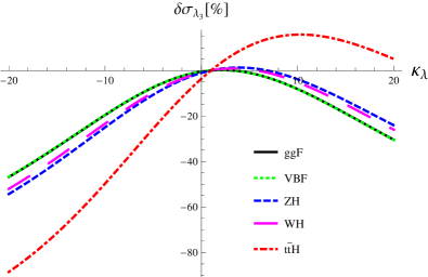
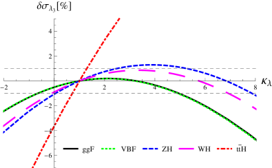
Figure 6: Dependence of $\delta\sigma_{\lambda_{3}}$ for the relevant production processes at the LHC as a function of $\kappa_{\lambda}$ in the range $|\kappa_{\lambda}|\leq 20$ (left) and zoomed in the region $-2<\kappa_{\lambda}<8$ (right). The style and colour conventions of the lines are: $gg{\rm F}$ = solid black, $t\bar{t}H$ = dash-dotted red, VBF = dotted green, $ZH$ = dashed blue, $WH$ = long-dashed magenta. The black dashed horizontal lines in the right plot correspond to $\pm 1\%$.

In Fig. 6 we plot $\delta\sigma_{\lambda_{3}}$ as a function of $\kappa_{\lambda}$ for the relevant production processes at the LHC, namely, gluon–gluon fusion, vector-boson-fusion, Higgs-strahlung ($WH$ and $ZH$) and $t\bar{t}H$ production. In the plot on left we display the $\delta\sigma_{\lambda_{3}}$ corrections for the various processes in the full range of validity of our calculation, $-20\lesssim\kappa_{\lambda}\lesssim 20$, while in the plot on the right we zoom the region $-2<\kappa_{\lambda}<8$, where corrections are within $5\%$ in absolute value for all processes but $t\bar{t}H$.

As can be seen, $t\bar{t}H$ receives positive sizeable corrections ($\sim 20\%$ at $\kappa_{\lambda}\sim 10$), thanks to the large value of $C_{1}^{\sigma}(t\bar{t}H)$. For all the other production processes large corrections can only be negative and only for large value of $|\kappa_{\lambda}|$. The plots on the right of Fig. 6 shows that $\delta\sigma_{\lambda_{3}}$ remains at the percent level for a quite extended range for the $gg{\rm F}$, VBF and $VH$ production modes. Moreover, for these processes, $\delta\sigma_{\lambda_{3}}$ can be zero for values of $\kappa_{\lambda}\neq 1$, i.e., different from the SM prediction. In particular, in the case of gluon-gluon fusion and VBF, the SM is degenerate with $\kappa_{\lambda}\sim 3$, while in the case of $VH$ production the SM is degenerate with $\kappa_{\lambda}\sim 6$. The fact that the degeneracy appears at different values $\kappa_{\lambda}$ for different processes is important in order to be able to lift it.

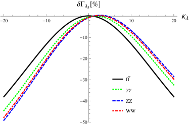
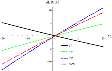
Figure 7: Dependence of $\delta\Gamma_{\lambda_{3}}$ for the relevant decay widths (right) and corresponding $\delta{\rm BR}_{\lambda_{3}}$ as defined in Eq. (15) (left). The solid black line represents $\Gamma_{f\bar{f}}$, the long-dashed red line $\Gamma_{\scriptscriptstyle WW}$, the dashed blue line $\Gamma_{\scriptscriptstyle ZZ}$ and the dotted green line $\Gamma_{\gamma\gamma}$.

The results for the decay widths and branching ratios are shown Fig. 7. We plot (left) $\delta\Sigma_{\lambda_{3}}$ as a function of $\kappa_{\lambda}$ for the decay widths of the relevant modes at the LHC, which we denote as $\delta\Gamma_{\lambda_{3}}$, and we show (right) the analogous quantity ($\delta{\rm BR}_{\lambda_{3}}$) for the Branching Ratios (BRs). The quantity $\delta{\rm BR}_{\lambda_{3}}(i)$ for the Higgs decay into the final-state $i$ can be conveniently written as

$$\delta{\rm BR}_{\lambda_{3}}(i)=\frac{(\kappa_{\lambda}-1)(C^{\Gamma}_{1}(i)-C_{1}^{\Gamma_{\rm tot}})}{1+(\kappa_{\lambda}-1)C_{1}^{\Gamma_{\rm tot}}}\,,$$ (15)

where we have defined $C_{1}^{\Gamma_{\rm tot}}\equiv\,\sum_{j}{\rm BR}^{\rm SM}(j)C^{\Gamma}_{1}(j)$ and with our input parameters $C_{1}^{\Gamma_{\rm tot}}=2.3\cdot 10^{-3}$. The quantity $C_{1}^{\Gamma_{\rm tot}}$, which actually is the $C_{1}$ term for the total decay width, is very small since $C^{\Gamma}_{1}(b\bar{b})=0$ and $b\bar{b}$ is the dominant decay channel. Note that, although the $H\rightarrow gg$ decay is not phenomenologically relevant, the total decay width does depend on $\delta\Gamma_{\lambda_{3}}(gg)$, since $\Gamma_{gg}$ yields a non-negligible fraction (8.5 %) of $\Gamma_{\rm tot}$.

Figure 7 shows that the corrections to the partial widths can reach up to $-40\%$ or $-50\%$ for $\kappa_{\lambda}\sim-20$, while for $\kappa_{\lambda}>0$ the corrections are smaller due to the different sign of the contributions depending on $C^{\Gamma}_{1}$ and $C_{2}$. The only exception is $\delta\Gamma_{\lambda_{3}}({f\bar{f}})$, which is symmetric since $C^{\Gamma}_{1}(f\bar{f})$=0. On the other hand, the corrections to the branching ratios $\delta{\rm BR}_{\lambda_{3}}$, which are more important than $\delta\Gamma_{\lambda_{3}}$ from a phenomenological point of view, are much smaller, reaching up to $\sim 10\%$ for ${\rm BR}(ZZ)$. The reasons behind the smallness of the $\delta{\rm BR}_{\lambda_{3}}$ are two. First, as explicitly shown in Eq. (15) $\delta{\rm BR}_{\lambda_{3}}$ depends only linearly upon $\kappa_{\lambda}$, since the contribution of the wave function renormalisation constant cancels in the ratio. Second, the $C_{1}$ coefficients have the same sign and therefore there is a partial cancellation in the ratio. In any case, it is interesting to note that in the range of $\kappa_{\lambda}$ shown in the right-hand plot of Fig. 6, apart from $t\bar{t}H$, the terms $\delta{\rm BR}_{\lambda_{3}}$ are of the same size or larger than $\delta\sigma_{\lambda_{3}}$. In other words, in the range close to the SM predictions, the decays modes are more sensitive to $\kappa_{\lambda}$ than the production processes.

5 Constrains on $\lambda_{3}$: present and future

In this section we describe the method and the results of a simplified fit we have performed in order to estimate the limits that can be set on $\kappa_{\lambda}$ with our approach. Our analysis is based on the experimental results presented in Tab. 8 of Ref. Khachatryan:2016vau . We also estimate the expected limits that could be obtained at LHC Run-II at 300 fb^-1 and 3000 fb^-1 of luminosity.

The key aspect of our approach is that the predictions for all the available production and decay channels depend on a single parameter ($\kappa_{\lambda}$) and therefore a global fit can be in principle very powerful in constraining the Higgs trilinear coupling. As our aim is mostly illustrative, we want to assess the competitiveness of our method rather than trying to obtain the best and most robust bounds. To this purpose, we make a series of simplifying approximations. For example, being usually quite small (see Fig. 7 of Ref. Khachatryan:2016vau ), we ignore correlations between the different uncertainties of a single measurement or between the measurements of the different observables.

The basic inputs of our analysis are the signal strength parameters $\mu_{i}^{f}$, which are defined for any specific combination of production and decay channel $i\to H\to f$ as

$$\mu_{i}^{f}\equiv\mu_{i}\times\mu^{f}=\frac{\sigma(i)}{\sigma(i)^{\rm SM}}\times\frac{{\rm BR}(f)}{{\rm BR}^{\rm SM}(f)}~{}.$$ (16)

The quantities $\mu_{i}$ and $\mu^{f}$ are the production cross section $\sigma(i)$ ($i=$ $gg{\rm F}$, VBF, $WH$, $ZH$, $t\bar{t}H$) and the ${\rm BR}(f)$ $(f=\gamma\gamma,ZZ,WW,b\bar{b},\tau\tau)$ normalised to their SM values, respectively. Assuming on-shell production, the product $\mu_{i}\times\mu^{f}$ is therefore the rate for the $i\to H\to f$ process normalised to the corresponding SM prediction.

Using Eq. (6) and Eq. (15), $\mu_{i}$ and $\mu^{f}$, which enter the definition of $\mu_{i}^{f}$ in Eq. (16), can be expressed as

$$\mu_{i} = 1+\delta\sigma_{\lambda_{3}}(i)\,,$$

$$\mu^{f} = 1+\delta{\rm BR}_{\lambda_{3}}(f)\,.$$ (17)

By definition, $\mu_{i}^{f}=\mu_{i}=\mu^{f}=1$ in the SM.

In the following we denote the measured signal strengths as $\bar{\mu}_{i}^{f}$. Given a collection of $\bar{\mu}_{i}^{f}$ measurements $\{\bar{\mu}_{i}^{f}\}$, we define as best value of $\kappa_{\lambda}$ the one that minimises the $\chi^{2}(\kappa_{\lambda})$ function defined as

$$\chi^{2}(\kappa_{\lambda})\equiv\sum_{\bar{\mu}_{i}^{f}\in\{\bar{\mu}_{i}^{f}\}}\frac{(\mu_{i}^{f}(\kappa_{\lambda})-\bar{\mu}_{i}^{f})^{2}}{(\Delta_{i}^{f}(\kappa_{\lambda}))^{2}}\,,$$ (18)

where $\mu_{i}^{f}(\kappa_{\lambda})$ is obtained using Eqs. (16) and (17), and $\Delta_{i}^{f}(\kappa_{\lambda})$ is the total uncertainty of $\mu_{i}^{f}$. Different sources of uncertainties enter in the determination of $\Delta_{i}^{f}(\kappa_{\lambda})$, namely, the experimental uncertainty in the measurement of $\mu_{i}^{f}$, the SM theory uncertainties associated to the particular channel $\mu_{i}\times\mu^{f}$ (scale, PDFs and $\alpha_{s}$), and the $\kappa_{\lambda}$-dependent uncertainty associated to missing higher orders, the $\mathcal{O}(\kappa_{\lambda}^{3}\alpha^{2})$ terms discussed in Sec. 2. The first two types of uncertainty are reported already combined in Ref. Khachatryan:2016vau , and divided in experimental and theoretical errors in Ref. Peskin:2013xra . For the third type of uncertainty, we adopt the parametrization $\frac{1}{\sqrt{3}}\kappa_{\lambda}^{3}C_{1}\delta Z_{H}$, where the $C_{1}$ depends on the observable and $\delta Z_{H}$ is defined in Eq. (3). It has to be kept in mind, however, that the results of our analysis show a very mild dependence on this uncertainty. 

	$H\rightarrow\gamma\gamma$	$H\rightarrow ZZ$	$H\rightarrow WW$	$H\rightarrow\tau\tau$	$H\rightarrow b\bar{b}$
$gg{\rm F}$	P1,2,3,4; F1,2	P1,2,3,4; F1,2	P1,2,3,4; F1,2	P1,2,3,4; F1	—
VBF	P2,3,4; F1,2	P2,3,4; F1,2	P2,3,4; F1,2	P2,3,4; F1,2	—
$WH$	P3,4	—	P3,4	P3,4	P3,4;F1,2
$ZH$	P3,4	—	P3,4	P3,4	P3,4
$t\bar{t}H$	P4; F1,2	—	P4	P4	P3,4;F1,2

Table 5: Combinations of production and decay modes used in the different analyses. Each P_n identifies one of our four different sets of present data taken from Ref. Khachatryan:2016vau . F₁ and F₂ respectively correspond to the future scenarios “CMS-II” (300 fb^-1) and “CMS-HL-II” (3000 fb^-1) as presented in Tab. 1 of Ref. Peskin:2013xra .

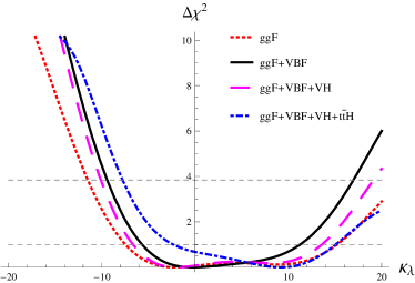
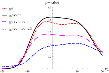
Figure 8: Left: $\chi^{2}$ for the different sets of observables presented in Tab. 5: the dotted red line represents P₁, the solid black line P₂, the dashed magenta line P₃, and the blue dash-dotted line P₄. The two horizontal lines represent $\Delta\chi^{2}=1$ and $\Delta\chi^{2}=3.84$. Right: corresponding $p$-value. The various P_n data sets are colour-coded in the same way. The horizontal line is $p=0.05$.

In order to evaluate the impact of the different production channels on the fit to the present data, we consider four different sets (P_n), with an increasing number of included production channels:

• P₁: $gg{\rm F}$,

• P₂: $gg{\rm F}$+VBF,

• P₃: $gg{\rm F}$+VBF+$VH$,

• P₄: $gg{\rm F}$+VBF+$VH$+${t\bar{t}H}$.

For the future scenarios (F_n), we consider

• F₁: “CMS-II” (300 fb^-1),

• F₂: “CMS-HL-II” (3000 fb^-1),

as presented in Tab. 1 of Ref. Peskin:2013xra . A summary of the sets of data used in each fit is presented in Tab. 5.

As shown in Fig. 8, we identify the $1\sigma$ and $2\sigma$ intervals assuming a $\chi^{2}$ distribution. Following this procedure and using the gluon-gluon-fusion and VBF data from Tab. 8 of Ref. Khachatryan:2016vau (scenario P₂ in Tab. 5) we obtain

$$\kappa_{\lambda}^{\rm best}=-0.24\,,~{}~{}~{}~{}~{}~{}\kappa_{\lambda}^{1\sigma}=[-5.6,11.2]\,,~{}~{}~{}~{}~{}~{}\kappa_{\lambda}^{2\sigma}=[-9.4,17.0]\,,$$ (19)

where the $\kappa_{\lambda}^{\rm best}$ is the best value and $\kappa_{\lambda}^{1\sigma}$, $\kappa_{\lambda}^{2\sigma}$ are respectively the $1\sigma$ and $2\sigma$ intervals. The choice of P₂ as reference set is motivated by the measured significance for the different production processes, which in the 8 TeV analyses is above $5\sigma$ only for $gg{\rm F}$ and VBF (see Tab. 14 in Ref. Khachatryan:2016vau ). Moreover, P₂ returns the most stringent values for $\kappa_{\lambda}^{1\sigma}$ and $\kappa_{\lambda}^{2\sigma}$. The other data sets presented in Tab. 5 are reported in Fig. 8. Notice how the minimum of the distribution in the figure jumps to $\sim$ 10 when the $t\bar{t}H$ production channel is included. This effect originates from the anomalous values presented in Ref. Khachatryan:2016vau for $\bar{\mu}_{t\bar{t}H}^{f}$, especially with $f=WW$. Similarly, the low compatibility of $\bar{\mu}_{VH}^{f}$ with SM predictions is the reason behind larger $\kappa_{\lambda}^{1\sigma}$ and $\kappa_{\lambda}^{2\sigma}$ intervals in P₃.

In order to ascertain the goodness of our fit, we computed the $p$-value as a function of $\kappa_{\lambda}$:

$$\text{$p$-value}(\kappa_{\lambda})=1-F_{\chi^{2}_{(n)}}(\chi^{2}(\kappa_{\lambda}))\,,$$ (20)

where $F_{\chi^{2}_{(n)}}(\chi^{2}(\kappa_{\lambda}))$ is the cumulative distribution function for a $\chi^{2}$ distribution with $n$ degrees of freedom, computed at $\chi^{2}(\kappa_{\lambda})$. In the right-hand side of Fig. 8 we report the $p$-value$(\kappa_{\lambda})$ corresponding to different data sets. Requiring that $p>0.05$, we are able to exclude, at more than $2\sigma$, that a model with an anomalous coupling $\kappa_{\lambda}<-14.3$ can explain the data in P₂.

We repeat the same procedure for ATLAS and CMS at 300 fb^-1 and 3000 fb^-1, using the uncertainties reported in Tab. 1 of Peskin:2013xra and, as a first step, assuming that the central value of the measurements in every channel coincides with the predictions of the SM. In Fig. 9 we report the two cases “CMS-II” (300 fb^-1) and “CMS-HL-II” (3000 fb^-1).

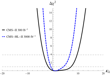
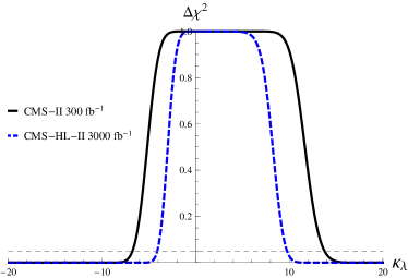
Figure 9: In the left and right plots, respectively $\chi^{2}(\kappa_{\lambda})$ and $p$-value$(\kappa_{\lambda})$ for “CMS-II” (solid black line) and “CMS-HL-II” (blue dashed line)

Within this approach, best values are by definition: $\kappa_{\lambda}^{\rm best}=1$. For the $1\sigma$ and $2\sigma$ intervals, and for the region where the $p$-value is larger than $0.05$, we find that the “CMS-II” (300 fb^-1) case gives

$$\kappa_{\lambda}^{1\sigma}=[-1.8,7.3]\,,~{}~{}~{}~{}\kappa_{\lambda}^{2\sigma}=[-3.5,9.6]\,,~{}~{}~{}~{}\kappa_{\lambda}^{p>0.05}=[-6.7,13.8]\,,$$ (21)

while for the “CMS-HL-II” (3000 fb^-1) we obtain

$$\kappa_{\lambda}^{1\sigma}=[-0.7,4.2]\,,~{}~{}~{}~{}\kappa_{\lambda}^{2\sigma}=[-2.0,6.8]\,,~{}~{}~{}~{}\kappa_{\lambda}^{p>0.05}=[-4.1,9.8]\,.$$ (22)

This simplified approach provides a first (rough) idea of the typical intervals that can be expected. A more reliable approach consists of considering, still within the SM assumption, all the possible central values that could be measured. To this aim, we produce a collection of pseudo-measurements $\{\bar{\mu}_{i}^{f}\}$, where each $\bar{\mu}_{i}^{f}$ is randomly generated with a gaussian distribution around the SM with a standard deviation equal to the experimental uncertainty cited in Tab. 1 of Peskin:2013xra . For each pseudo-experiment we perform a fit and we determine $\kappa_{\lambda}^{\rm best}$ and the $\kappa_{\lambda}^{1\sigma}$, $\kappa_{\lambda}^{2\sigma}$ and $\kappa_{\lambda}^{p>0.05}$ intervals. In Figs. 10 and 11 we report the results out of a collection of $n=10000$ pseudo-experiment. Frequency histograms together with corresponding mean and median values are provided for $\kappa_{\lambda}^{\rm best}$ and all the extremes and widths of the $\kappa_{\lambda}^{1\sigma}$, $\kappa_{\lambda}^{2\sigma}$ and $\kappa_{\lambda}^{p>0.05}$ intervals. From these plots it is clear that most likely the limits written in Eq. (21) and (22) are pessimistic, and the LHC should be able to put even stronger bounds.

Figure 10: Histograms for “CMS-II” (300 fb^-1). The distributions represented are, from left to right and from top to bottom: 1) best values, 2) $1\sigma$ region lower limit, 3) $1\sigma$ region upper limit, 4) $2\sigma$ region lower limit, 5) $2\sigma$ region upper limit, 6) $p>0.05$ region lower limit, 7) $p>0.05$ region upper limit, 8) $1\sigma$ region width, 9) $2\sigma$ region width, 10) $p>0.05$ region width.

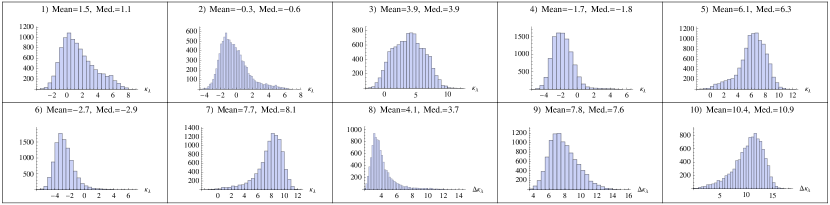
Figure 11: As Fig. 10 for “CMS-HL-II” (3000 fb^-1).

As a last exercise, we consider an optimistic scenario where the quadratic sum of the experimental and theoretical uncertainties amounts to one percent in total. To this aim we employ the observables included in the data sets P_1,2,3,4, and assume, as first step, that the measured signal strength is the one of the SM with an associated $0.01$ relative uncertainty. In Fig. 12 we report the obtained $\chi^{2}(\kappa_{\lambda})$ and $p$-value$(\kappa_{\lambda})$. As expected, a precise measurement of the $t\bar{t}H$ would lead to a sizeable improvement in the fit. For example, we find that for the scenario P₄

$$\kappa_{\lambda}^{1\sigma}=[0.86,1.14]\,,~{}~{}~{}~{}\kappa_{\lambda}^{2\sigma}=[0.74,1.28]\,,~{}~{}~{}~{}\kappa_{\lambda}^{p>0.05}=[0.28,1.80]\,.$$ (23)

Considering as before $n=10000$ pseudo-measurements, the histograms analogous to those in Fig. 10 and 11 are shown in Fig. 13. Again, we find the indication that, most-likely, in this optimistic scenario stronger bounds than those reported in Eq. (23) could be set.

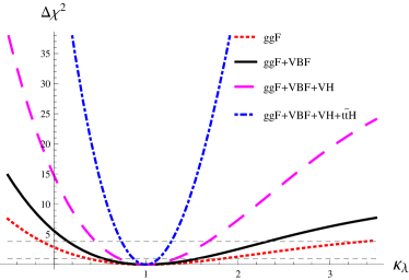
Figure 12: In the left and right plots, respectively $\chi^{2}(\kappa_{\lambda})$ and $p$-value$(\kappa_{\lambda})$ for the P_1,2,3,4 scenarios with relative uncertainties set at $0.01$.

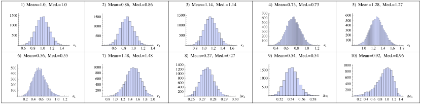
Figure 13: As Fig. 10 for the P₄ scenario with relative uncertainties set to 0.01.

6 Conclusions

The structure and properties of the scalar sector encompassing the observed Higgs boson are largely unexplored and their determination is one of the major goals of the LHC and future colliders. In the standard model the Higgs self couplings, trilinear and quartic, are fixed by the Higgs mass, yet they could be different in scenarios featuring extended scalar sectors or new strong dynamics. The most-beaten path to determine the trilinear coupling is via the direct measurement of Higgs pair production total cross sections and differential distributions. However, the small expected rates, the mild dependence of the cross section on the trilinear coupling and the difficulty of selecting signal from backgrounds make this path very arduous.

In this work we have put forward an alternative method, which relies on the effects that loops featuring an anomalous trilinear coupling would imprint on single Higgs production channels at the LHC. We have calculated the contributions arising at NLO on all the phenomenologically relevant single Higgs production ($gg{\rm F}$, VBF, $WH$, $ZH$, $t\bar{t}H$) and decay ($\gamma\gamma$, $WW^{*}/ZZ^{*}\to 4f$, $b\bar{b}$, $\tau\tau$) modes at the LHC. Remarkably, we have found that the $\lambda_{3}$ dependence is different for each channel (production times decay) and is also affected by the final state kinematic configurations. We have then estimated the sensitivity to the trilinear coupling via a one-parameter fit to the complete set of single Higgs inclusive measurements at the LHC 8 TeV. The bounds obtained are found to be competitive with the current ones obtained from Higgs pair production. We have also estimated the constraints that can be obtained at the end of the current Run II and also in the HL phase with an integrated luminosity of 3000 fb^-1 expected. In all cases, the determination of the Higgs self coupling via loop effects is competitive with the direct determination and will provide complementary information.

We remark that when an analysis based on a single observable is made, the effects induced by a modification of the trilinear coupling cannot be distinguished from those induced by an overall rescaling factor of the relevant Higgs coupling, like a $\kappa_{f}$ or $\kappa_{V}$ factor. Instead, the simultaneous analysis of several observables allows the identification of the different sources of the various effects. We also note that, even though not exploited in this first study, differential information from single Higgs production and/or decays could also be used to improve the sensitivity.

The indirect approach outlined in this work relies on the assumption that the leading effects from physics beyond the Standard Model affect the Higgs potential only, i.e., the couplings to fermions and vector bosons are not (or just mildly) affected by new physics at the tree level. Admittedly, this might be a limitation for studying some specific new physics scenarios. However, this assumption is not a requirement for our method to be applied. As information on the Higgs couplings to vector boson and the top quark will become more accurate, one could think of progressively lift the condition on the other Higgs couplings to be SM and allow for tree-level deviations in the global fit. A first straightforward step will be the extension to a three-parameter ($\kappa_{V},\kappa_{f},\kappa_{\lambda}$) fit, being $\kappa_{V}$, $\kappa_{f}$ the universal rescaling factors of the fermion/boson Higgs couplings. A further step will be the study of the additional sensitivity given by the inclusion of collider energy and differential observable dependences in the fit. Work in this direction is in progress.

In this work we have chosen to present the results in the context of the $\kappa$-framework, because with the current sensitivities only rather large deviations from the SM can be probed. Moreover, in this way our results can be straightforwardly implemented in the experimental global analyses Khachatryan:2016vau , which are also currently based on the $\kappa$-framework. The next step will be the interpretation of our loop calculations in the context of an effective field theory including at least dimension-6 operators. In this context, issues such as how many independent observables are needed to lift all possible degeneracies in the effects induced by different operators (at tree- and one-loop level), need further investigation.

Appendix A Comparison with the EFT approach

The SM potential for the Higgs doublet field reads

$$V^{\rm SM}(\Phi)=-\mu^{2}(\Phi^{\dagger}\Phi)+\lambda(\Phi^{\dagger}\Phi)^{2}\,,\qquad\Phi=\frac{1}{\sqrt{2}}\begin{pmatrix}\phi^{+}\cr v+H+i\phi^{0}\,\end{pmatrix}\ ,$$ (A.1)

and can be modified by adding the dimension-6 operators $(\Phi^{\dagger}\Phi)^{3}$,

$$V^{\rm dim-6}(\Phi)=V^{\rm SM}(\Phi)+\frac{c_{6}}{v^{2}}(\Phi^{\dagger}\Phi)^{3}\,,$$ (A.2)

where the normalization of the operator $(\Phi^{\dagger}\Phi)^{3}$ is $v=(\sqrt{2}G_{\mu})^{-1/2}=246~{}\,\textrm{GeV}$. The relations among $m_{\scriptscriptstyle H}$, $v$, $\mu$ and $\lambda$ are different in $V^{\rm SM}(\Phi)$ and $V^{\rm dim-6}(\Phi)$. We determine $\lambda$ and $\mu$ as function of the measured quantities, $m_{\scriptscriptstyle H}$ and $v$, and of the new parameter $c_{6}$. Once all the dependences are expressed as function of $m_{\scriptscriptstyle H}$, $v$ and $c_{6}$, we can derive the value of the coefficient in front of $H^{3}$ which in the paper is called $\lambda_{3}$, as well as the coefficient in front of the quartic term $H^{4}$, which is denoted as $\lambda_{4}$. The SM relations are recovered by setting $c_{6}=0$.

With the condition $\frac{dV^{\rm dim-6}(\Phi)}{d\Phi}\Big{|}_{|\Phi|=v/\sqrt{2}}=0$ , one obtains

$$v=\frac{2\mu}{\sqrt{4\lambda+3c_{6}}}~{}\rightarrow~{}\mu=\frac{1}{2}v\sqrt{4\lambda+3c_{6}}\,,$$ (A.3)

which after Electroweak Symmetry Breaking implies

$$m_{\scriptscriptstyle H}^{2}=v^{2}(2\lambda+3c_{6})\,\rightarrow\lambda=\frac{m_{\scriptscriptstyle H}^{2}}{2v^{2}}-\frac{3c_{6}}{2}\,,$$ (A.4)

and

$$c_{H^{3}}\equiv v\lambda_{3}=v\left(\lambda+\frac{5}{2}c_{6}\right)=\frac{m_{\scriptscriptstyle H}^{2}}{2v}+c_{6}v\rightarrow\kappa_{\lambda}=1+\frac{2c_{6}v^{2}}{m_{\scriptscriptstyle H}^{2}}\,.$$ (A.5)

At a first sight, the linear relation in Eq. (A.5) seems to imply that with the potential $V^{\rm dim-6}(\Phi)$ any value of $\lambda_{3}$ can be obtained. However, one can require that the potential is bounded from below ($c_{6}>0$) and that $v$ is the global minimum. The latter condition had been already discussed in Ref. Grojean:2004xa and can be easily derived substituting in the potential of Eq. (A.2) $\mu$ and $\lambda$ with $m_{\scriptscriptstyle H}$ and $v$ via Eqs. (A.3) and (A.4):

$$V^{\rm dim-6}(\Phi)=\left(-\frac{m_{\scriptscriptstyle H}^{2}}{2}+\frac{3}{4}c_{6}v^{2}\right)\Phi^{\dagger}\Phi\ +\left(\frac{m_{\scriptscriptstyle H}^{2}}{2v^{2}}-\frac{3}{2}c_{6}\right)(\Phi^{\dagger}\Phi)^{2}+\frac{c_{6}}{v^{2}}(\Phi^{\dagger}\Phi)^{3}\,.$$ (A.6)

Since $\Phi=0$ can be a local minimum, the condition that $v$ is a global minimum requires

$$V^{\rm dim-6}(v/\sqrt{2})=\frac{c_{6}v^{4}-m_{\scriptscriptstyle H}^{2}v^{2}}{8}<0=V^{\rm dim-6}(0)\,.$$ (A.7)

or $c_{6}<m_{\scriptscriptstyle H}^{2}/v^{2}$. Thus, with the inclusion of only the $(\Phi^{\dagger}\Phi)^{3}$ operator in the SM Lagrangian $\kappa_{\lambda}$ is constrained to be in the range

$$1<\kappa_{\lambda}<3\,.$$ (A.8)

It is worth to notice that this bound has been derived without any assumption on the size $c_{6}$, which in an EFT approach would be subject to further constraints depending on the scale of new physics $\Lambda$.

In a general EFT approach in principle the value of $\lambda_{3}$ can be affected also by another dimension-6 operator, namely, $\frac{c_{\Phi}}{2v^{2}}\partial^{\mu}(\Phi^{\dagger}\Phi)\partial_{\mu}(\Phi^{\dagger}\Phi)$. However, other couplings of the Higgs boson would also be affected by this operator, such as the coupling with the $Z$ boson and with the fermions. Thus, these effects would be already present at LO in single-Higgs production and would be in general much larger than the effects induced by an anomalous $\lambda_{3}$ coupling. Only for values $1<\kappa_{\lambda}<3$ and assuming $c_{\Phi}=0$ the results obtained in this paper can be converted to values of $c_{6}$ via eq. (A.5). Moreover, in the EFT approach, Wilson coefficients at the scale $\Lambda$ are typically expected to be smaller in absolute value than $4\pi$. This requirement would additionally set the constraint

$$c_{6}<4\pi\frac{v^{2}}{\Lambda^{2}}\rightarrow 1<\kappa_{\lambda}<\min\left(3\,,1+8\pi\frac{v^{4}}{m_{\scriptscriptstyle H}^{2}\Lambda^{2}}\right)\,.$$ (A.9)

Analogously to what has been done for the trilinear coupling, we can define $\lambda_{4}\equiv\kappa_{\lambda_{4}}\lambda_{4}^{\rm SM}$ finding

$$\kappa_{\lambda_{4}}=1+\frac{12c_{6}v^{2}}{m_{\scriptscriptstyle H}^{2}}\,,$$ (A.10)

which implies

$$\kappa_{\lambda_{4}}=6\kappa_{\lambda}-5\rightarrow 1<\kappa_{\lambda_{4}}<\min\left(13\,,1+48\pi\frac{v^{4}}{m_{\scriptscriptstyle H}^{2}\Lambda^{2}}\right)\,\,,$$ (A.11)

since, with the $V^{\rm dim-6}(\Phi)$ potential, $\lambda_{4}$ is a prediction fixed by $m_{\scriptscriptstyle H},v$ and $\lambda_{3}$.

As last comments concerning the potential in Eq. (A.2), we want to stress that the constraints in Eqs. (A.8)-(A.9), the relation between $\lambda_{3}$ and $\lambda_{4}$ and thus also the constraints on $\lambda_{4}$ in Eq. (A.11) are parametrisation independent, i.e., they are not altered by the choice of normalisation of the $(\Phi^{\dagger}\Phi)^{3}$ operator. Using for instance, the normalisation $\bar{c}_{6}\frac{\lambda}{v^{2}}$ of Ref. Gorbahn:2016uoy , Eqs. (A.3)-(A.5) and Eq. (A.10) would change, namely:

$$m_{\scriptscriptstyle H}^{2}=v^{2}\lambda(2+3c_{6})\rightarrow\lambda=\frac{m_{\scriptscriptstyle H}^{2}}{v^{2}(2+3\bar{c}_{6})}\,$$ (A.12)

$$\kappa_{\lambda}=\frac{2+5\bar{c}_{6}}{2+3\bar{c}_{6}}\,,$$ (A.13)

$$\kappa_{\lambda_{4}}=\frac{2+15\bar{c}_{6}}{2+3\bar{c}_{6}}\,.$$ (A.14)

Equations (A.13) and (A.14) can be easily related to (A.5) and (A.10) in the limit $c_{6}$ or $\bar{c}_{6}\rightarrow 0$, i.e., $\kappa_{\lambda},~{}\kappa_{\lambda_{4}}\sim 1$. On the other hand, with this parametrisation, it is less obvious how to determine the maximal and minimal possible values for $\kappa_{\lambda}$. In any case, imposing the conditions that the potential is bounded from below and that $v$ is the global minimum, it is possible to recover the bound $1<\kappa_{\lambda}<3$, confirming its independence on the choice of normalisation of the $(\Phi^{\dagger}\Phi)^{3}$ term.

As a final exercise, we consider the extension of the SM potential $V^{\rm SM}$

$$V^{\rm dim-8}(\Phi)=V^{\rm SM}(\Phi)+\frac{c_{6}}{v^{2}}(\Phi^{\dagger}\Phi)^{3}+\frac{c_{8}}{v^{4}}(\Phi^{\dagger}\Phi)^{4}\,,$$ (A.15)

where besides the $(\Phi^{\dagger}\Phi)^{3}$ term also the $(\Phi^{\dagger}\Phi)^{4}$ is included. Relations corresponding to those in Eqs. (A.3)-(A.5) and (A.10) can be derived in a completely analogous way. We write them directly as function of $m_{\scriptscriptstyle H},\lambda,c_{6}$ and $c_{8}$, where by setting $c_{8}=0$ one recovers the analogous ones for the potential in Eq. A.2:

$$\mu^{2}=\frac{m_{\scriptscriptstyle H}^{2}}{2}-\frac{3c_{6}}{4}v^{2}-c_{8}v^{2}\,,$$ (A.16)

$$\lambda=\frac{m_{\scriptscriptstyle H}^{2}}{2v^{2}}-\frac{3c_{6}}{2}-\frac{3c_{8}}{2}\,,$$ (A.17)

$$\kappa_{\lambda}=1+\frac{(2c_{6}+4c_{8})v^{2}}{m_{\scriptscriptstyle H}^{2}}\,,$$ (A.18)

$$\kappa_{\lambda_{4}}=1+\frac{(12c_{6}+32c_{8})v^{2}}{m_{\scriptscriptstyle H}^{2}}\,.$$ (A.19)

At variance with the case of $V^{\rm dim-6}(\Phi)$, with the inclusion of the $\frac{c_{8}}{v^{4}}(\Phi^{\dagger}\Phi)^{4}$ term the quantity $\kappa_{\lambda_{4}}$ is independent of $\kappa_{\lambda}$, i.e., $c_{6}$ and $c_{8}$ can be traded off with $\kappa_{\lambda}$ and $\kappa_{\lambda_{4}}$. The requirement that the potential is bounded from below implies $c_{8}>0$, which in conjunction with the requirement that the global minimum is located at $\Phi=v/\sqrt{2}$ implies

$$-4+4\kappa_{\lambda}+\kappa_{\lambda}^{2}<\kappa_{\lambda_{4}}<\frac{-31+30\kappa_{\lambda}+9\kappa_{\lambda}^{2}}{8}\,.$$ (A.20)

Thus, without any constraint on the size of $c_{6}$ and $c_{8}$, such as those coming from an EFT, $\kappa_{\lambda}$ is not bounded and $\kappa_{\lambda_{4}}$ is constrained by Eq. (A.20).

Appendix B $C_{1}$ terms for $\sigma(gg\rightarrow H)$ and $\Gamma(H\rightarrow\gamma\gamma)$

In this appendix we present the results for the $C_{1}$ factor in the gluon-gluon-fusion Higgs production and in the Higgs partial decay into two photons.

B.1 $\sigma(gg\rightarrow H)$

We write the SM gluon-gluon-fusion Higgs production partonic cross-section as

$$\sigma=\frac{G_{\mu}\alpha_{s}^{2}}{512\sqrt{2}\pi}|{\cal G}|^{2},$$ (B.1)

where ${\cal G}={\cal G}^{1l}+{\cal G}^{2l}+...$ with the lowest order contribution given by

$${\cal G}^{1l}=-\frac{4}{h_{t}}\left(2-\frac{1-4/h_{t}}{2}\log^{2}\left[\frac{\sqrt{1-4/h_{t}}-1}{\sqrt{1-4/h_{t}}+1}\right]\right),~{}~{}~{}~{}h_{t}\equiv\frac{m_{\scriptscriptstyle H}^{2}}{m_{t}^{2}}~{}.$$ (B.2)

The two-loop contribution can be written as: ${\cal G}^{2l}=K_{r}\,{\cal G}^{1l}+{\cal G}^{2l}_{1{\rm PI}}$ with ${\cal G}^{2l}_{1{\rm PI}}$ the contribution of the one-particle irreducible (1PI) vertex diagrams and

$$K_{r}\equiv\left[\frac{A_{\scriptscriptstyle WW}}{m_{\scriptscriptstyle W}^{2}}-V-B+(\delta Z_{H})_{\scriptscriptstyle{\rm SM}}\right]\,,$$ (B.3)

where $A_{\scriptscriptstyle WW}$ is the transverse part of the $W$ self-energy at zero momentum transverse, the quantities $V$ and $B$ represent the vertex and box corrections in the $\mu$-decay amplitude and $(\delta Z_{H})_{\scriptscriptstyle{\rm SM}}$ is the Higgs field wave function renormalisation constant in the SM.

In our scenario the modification of the Higgs wave function, represented by the $C_{2}$ coefficient, will affect the $K_{r}$ term while $C_{1}$ is extracted from the diagrams in Fig. 4 that contribute to ${\cal G}^{2l}_{1{\rm PI}}$.

Under the standard approximation of the factorisation of the EW corrections in $\sigma(gg\rightarrow H)$ we have for $C_{1}$

$$C_{1}^{\sigma}(gg{\rm F})=2\frac{{\cal G}^{2l}_{1{\rm PI},\,{\lambda_{3}^{\rm SM}}}}{{\cal G}^{1l}}\,,$$ (B.4)

where

$${\cal G}^{2l}_{1{\rm PI},\,{\lambda_{3}^{\rm SM}}} = \frac{G_{\mu}m_{\scriptscriptstyle H}^{2}}{2\,\sqrt{2}\pi^{2}}\left[\frac{-23+4\sqrt{3}\pi}{24}+\frac{1}{2}\log(h_{t})\right.$$ (B.5)

$$~{}~{}~{}~{}~{}+h_{t}\left(\frac{7}{480}(-37+4\sqrt{3}\pi)+\frac{7}{20}\log(h_{t})\right)$$

$$~{}~{}~{}~{}~{}+h_{t}^{2}\left(\frac{-464419+33810\sqrt{3}\pi}{2116800}+\frac{349}{2016}\log(h_{t})\right)$$

$$~{}~{}~{}~{}+\left.h_{t}^{3}\left(-\frac{31795373}{381024000}+\frac{13\pi}{1050\sqrt{3}}+\frac{1741}{21600}\log(h_{t})\right)\right]~{}.$$

B.2 $\Gamma(H\rightarrow\gamma\gamma)$

For $\Gamma(H\rightarrow\gamma\gamma)$ we have

$$\Gamma=\frac{G_{\mu}\alpha^{2}M_{h}^{3}}{128\sqrt{2}\pi^{3}}|F|^{2},$$ (B.6)

with ${\cal F}={\cal F}^{1l}+{\cal F}^{2l}+...$. The lowest order contribution is given by

$${\cal F}^{1l}=N_{c}Q^{2}{\cal G}^{1l}+2(1+\frac{6}{h_{\scriptscriptstyle W}})-\frac{6}{h_{\scriptscriptstyle W}}(1-\frac{2}{h_{\scriptscriptstyle W}})\log^{2}\left[\frac{\sqrt{1-4/h_{\scriptscriptstyle W}}-1}{\sqrt{1-4/h_{\scriptscriptstyle W}}+1}\right]\,,$$ (B.7)

with $Q=2/3,\>N_{c}=3$ and $h_{\scriptscriptstyle W}=m_{\scriptscriptstyle H}^{2}/m_{\scriptscriptstyle W}^{2}$.

The two-loop form factor ${\cal F}^{2l}$ can be decomposed in the same way as ${\cal G}^{2l}$ so that $C_{1}$ can be extracted from the 1PI diagrams in Figs.4 and 5) evaluated in the unitary gauge. We find

$$C_{1}^{\Gamma}(\gamma\gamma)=2\frac{{\cal F}^{2l}_{1{\rm PI},\,\lambda_{3}^{\rm SM}}}{{\cal F}^{1l}}\,.$$ (B.8)

where

$${\cal F}^{2l}_{1{\rm PI},\,\lambda_{3}^{\rm SM}} = N_{c}Q^{2}{\cal G}^{2l}_{\lambda_{3}^{\rm SM}}+\frac{G_{\mu}m_{\scriptscriptstyle W}^{2}}{2\,\sqrt{2}\pi^{2}}\Bigg{\{}p_{w}^{2}\bigg{[}-36+12h_{\scriptscriptstyle W}-15h_{\scriptscriptstyle W}^{2}+\frac{9}{2}h_{\scriptscriptstyle W}^{3}$$

$$- 12(6-46h_{\scriptscriptstyle W}+13h_{\scriptscriptstyle W}^{2})L_{w}+9(-8-12h_{\scriptscriptstyle W}-6h_{\scriptscriptstyle W}^{2}+3h_{\scriptscriptstyle W}^{3})\phi_{w}\bigg{]}$$

$$+ p_{w}^{4}\bigg{[}\frac{1}{30}(-38880+98640h_{\scriptscriptstyle W}-68384h_{\scriptscriptstyle W}^{2}+15204h_{\scriptscriptstyle W}^{3}+142h_{\scriptscriptstyle W}^{4}-308h_{\scriptscriptstyle W}^{5}+33h_{\scriptscriptstyle W}^{6})$$

$$- \frac{2}{15}(19440-26760h_{\scriptscriptstyle W}+15028h_{\scriptscriptstyle W}^{2}-7262h_{\scriptscriptstyle W}^{3}+1522h_{\scriptscriptstyle W}^{4}+57h_{\scriptscriptstyle W}^{5})L_{w}$$

$$+ 8(-324+500h_{\scriptscriptstyle W}-323h_{\scriptscriptstyle W}^{2}+102h_{\scriptscriptstyle W}^{3}-31h_{\scriptscriptstyle W}^{4}+7h_{\scriptscriptstyle W}^{5})\phi_{w}\bigg{]}$$

$$+ p_{w}^{6}\bigg{[}\frac{1}{945}(-38283840+84825216h_{\scriptscriptstyle W}-70055664h_{\scriptscriptstyle W}^{2}+18977592h_{\scriptscriptstyle W}^{3}-2081216h_{\scriptscriptstyle W}^{4}$$

$$+ 252530h_{\scriptscriptstyle W}^{5}-56436h_{\scriptscriptstyle W}^{6}+54710h_{\scriptscriptstyle W}^{7}-9158h_{\scriptscriptstyle W}^{8}+513h_{\scriptscriptstyle W}^{9})$$

$$- \frac{2}{105}(4253760-9166080h_{\scriptscriptstyle W}+8167712h_{\scriptscriptstyle W}^{2}-5453632h_{\scriptscriptstyle W}^{3}$$

$$+ 1553124h_{\scriptscriptstyle W}^{4}-298912h_{\scriptscriptstyle W}^{5}+78152h_{\scriptscriptstyle W}^{6}-3992h_{\scriptscriptstyle W}^{7}+171h_{\scriptscriptstyle W}^{8})L_{w}$$

$$+ \frac{8}{3}(-30384+70536h_{\scriptscriptstyle W}-69084h_{\scriptscriptstyle W}^{2}+34642h_{\scriptscriptstyle W}^{3}$$

$$- 13138h_{\scriptscriptstyle W}^{4}+2337h_{\scriptscriptstyle W}^{5}-82h_{\scriptscriptstyle W}^{6}+43h_{\scriptscriptstyle W}^{7})\phi_{w}\bigg{]}$$

$$+ p_{w}^{8}\bigg{[}\frac{1}{4725}(-6078844800+15433978560h_{\scriptscriptstyle W}$$

$$- 16158069376h_{\scriptscriptstyle W}^{2}+9535767472h_{\scriptscriptstyle W}^{3}$$

$$- 3860103960h_{\scriptscriptstyle W}^{4}+933792696h_{\scriptscriptstyle W}^{5}-198236360h_{\scriptscriptstyle W}^{6}+49562148h_{\scriptscriptstyle W}^{7}$$

$$+ 370584h_{\scriptscriptstyle W}^{8}-1829312h_{\scriptscriptstyle W}^{9}+410373h_{\scriptscriptstyle W}^{10}-40412h_{\scriptscriptstyle W}^{11}+1566h_{\scriptscriptstyle W}^{12})$$

$$- \frac{4}{1575}(1013140800-2714896800h_{\scriptscriptstyle W}$$

$$+ 3103464560h_{\scriptscriptstyle W}^{2}-1987417480h_{\scriptscriptstyle W}^{3}+754138872h_{\scriptscriptstyle W}^{4}$$

$$- 219727216h_{\scriptscriptstyle W}^{5}+5585768h_{\scriptscriptstyle W}^{6}+15961770h_{\scriptscriptstyle W}^{7}$$

$$- 1982560h_{\scriptscriptstyle W}^{8}+349052h_{\scriptscriptstyle W}^{9}-25056h_{\scriptscriptstyle W}^{10}+783h_{\scriptscriptstyle W}^{11})L_{w}$$

$$+ \frac{32}{15}(-1206120+3433040h_{\scriptscriptstyle W}-4226570h_{\scriptscriptstyle W}^{2}+2964582h_{\scriptscriptstyle W}^{3}-1314797h_{\scriptscriptstyle W}^{4}$$

$$+ 372126h_{\scriptscriptstyle W}^{5}-99064h_{\scriptscriptstyle W}^{6}+16782h_{\scriptscriptstyle W}^{7}+662h_{\scriptscriptstyle W}^{8}+121h_{\scriptscriptstyle W}^{9})\phi_{w}\bigg{]}\Bigg{\}}\,,$$

where $p_{w}^{2}=\frac{q^{2}}{4m_{\scriptscriptstyle W}^{2}}\frac{1}{h_{\scriptscriptstyle W}(h_{\scriptscriptstyle W}-4)^{2}}$, with $q^{2}$ the squared external momentum of the Higgs field that is put on the mass-shell at the end of the calculation, $q^{2}=m_{\scriptscriptstyle H}^{2}$, and $L_{w}=\frac{\log(h_{w})}{(h_{\scriptscriptstyle W}-4)}$, $\phi_{w}=\phi(\frac{h_{w}}{4})\frac{1}{h_{\scriptscriptstyle W}(h_{\scriptscriptstyle W}-4)}$, with

$$\phi(z)=4\sqrt{\frac{z}{1-z}}\ \text{Im}(\text{Li}_{2}(e^{i2\arcsin(\sqrt{z})}))~{}.$$ (B.9)

References

- (1) CMS collaboration, S. Chatrchyan et al., Observation of a new boson at a mass of 125 GeV with the CMS experiment at the LHC, Phys. Lett. B716 (2012) 30–61, [1207.7235].
- (2) ATLAS collaboration, G. Aad et al., Observation of a new particle in the search for the Standard Model Higgs boson with the ATLAS detector at the LHC, Phys.Lett. B716 (2012) 1–29, [1207.7214].
- (3) CMS collaboration, V. Khachatryan et al., Precise determination of the mass of the Higgs boson and tests of compatibility of its couplings with the standard model predictions using proton collisions at 7 and 8 TeV, Eur. Phys. J. C75 (2015) 212, [1412.8662].
- (4) ATLAS collaboration, G. Aad et al., Measurements of the Higgs boson production and decay rates and coupling strengths using pp collision data at and 8 TeV in the ATLAS experiment, Eur. Phys. J. C76 (2016) 6, [1507.04548].
- (5) ATLAS, CMS collaboration, G. Aad et al., Measurements of the Higgs boson production and decay rates and constraints on its couplings from a combined ATLAS and CMS analysis of the LHC collision data at 7 and 8 TeV, 1606.02266.
- (6) LHC Higgs Cross Section Working Group collaboration, A. David, A. Denner, M. Duehrssen, M. Grazzini, C. Grojean, G. Passarino et al., LHC HXSWG interim recommendations to explore the coupling structure of a Higgs-like particle, 1209.0040.
- (7) LHC Higgs Cross Section Working Group collaboration, J. R. Andersen et al., Handbook of LHC Higgs Cross Sections: 3. Higgs Properties, 1307.1347.
- (8) CMS collaboration, Projected Performance of an Upgraded CMS Detector at the LHC and HL-LHC: Contribution to the Snowmass Process, in Community Summer Study 2013: Snowmass on the Mississippi (CSS2013) Minneapolis, MN, USA, July 29-August 6, 2013, 2013. 1307.7135.
- (9) M. E. Peskin, Estimation of LHC and ILC Capabilities for Precision Higgs Boson Coupling Measurements, in Community Summer Study 2013: Snowmass on the Mississippi (CSS2013) Minneapolis, MN, USA, July 29-August 6, 2013, 2013. 1312.4974.
- (10) R. S. Gupta, H. Rzehak and J. D. Wells, How well do we need to measure the Higgs boson mass and self-coupling?, Phys. Rev. D88 (2013) 055024, [1305.6397].
- (11) A. Efrati and Y. Nir, What if , 1401.0935.
- (12) C. Anastasiou, C. Duhr, F. Dulat, E. Furlan, T. Gehrmann, F. Herzog et al., High precision determination of the gluon fusion Higgs boson cross-section at the LHC, 1602.00695.
- (13) D. de Florian and J. Mazzitelli, Higgs Boson Pair Production at Next-to-Next-to-Leading Order in QCD, Phys. Rev. Lett. 111 (2013) 201801, [1309.6594].
- (14) F. Maltoni, E. Vryonidou and M. Zaro, Top-quark mass effects in double and triple Higgs production in gluon-gluon fusion at NLO, JHEP 11 (2014) 079, [1408.6542].
- (15) S. Borowka, N. Greiner, G. Heinrich, S. Jones, M. Kerner, J. Schlenk et al., Higgs Boson Pair Production in Gluon Fusion at Next-to-Leading Order with Full Top-Quark Mass Dependence, Phys. Rev. Lett. 117 (2016) 012001, [1604.06447].
- (16) J. Baglio, A. Djouadi, R. Gröber, M. M. Mühlleitner, J. Quevillon and M. Spira, The measurement of the Higgs self-coupling at the LHC: theoretical status, JHEP 04 (2013) 151, [1212.5581].
- (17) R. Frederix, S. Frixione, V. Hirschi, F. Maltoni, O. Mattelaer, P. Torrielli et al., Higgs pair production at the LHC with NLO and parton-shower effects, Phys. Lett. B732 (2014) 142–149, [1401.7340].
- (18) U. Baur, T. Plehn and D. L. Rainwater, Probing the Higgs selfcoupling at hadron colliders using rare decays, Phys. Rev. D69 (2004) 053004, [hep-ph/0310056].
- (19) W. Yao, Studies of measuring Higgs self-coupling with at the future hadron colliders, in Community Summer Study 2013: Snowmass on the Mississippi (CSS2013) Minneapolis, MN, USA, July 29-August 6, 2013, 2013. 1308.6302.
- (20) V. Barger, L. L. Everett, C. B. Jackson and G. Shaughnessy, Higgs-Pair Production and Measurement of the Triscalar Coupling at LHC(8,14), Phys. Lett. B728 (2014) 433–436, [1311.2931].
- (21) A. Azatov, R. Contino, G. Panico and M. Son, Effective field theory analysis of double Higgs boson production via gluon fusion, Phys. Rev. D92 (2015) 035001, [1502.00539].
- (22) C.-T. Lu, J. Chang, K. Cheung and J. S. Lee, An exploratory study of Higgs-boson pair production, JHEP 08 (2015) 133, [1505.00957].
- (23) M. J. Dolan, C. Englert and M. Spannowsky, Higgs self-coupling measurements at the LHC, JHEP 10 (2012) 112, [1206.5001].
- (24) A. Papaefstathiou, L. L. Yang and J. Zurita, Higgs boson pair production at the LHC in the channel, Phys. Rev. D87 (2013) 011301, [1209.1489].
- (25) D. E. Ferreira de Lima, A. Papaefstathiou and M. Spannowsky, Standard model Higgs boson pair production in the ( )( ) final state, JHEP 08 (2014) 030, [1404.7139].
- (26) D. Wardrope, E. Jansen, N. Konstantinidis, B. Cooper, R. Falla and N. Norjoharuddeen, Non-resonant Higgs-pair production in the final state at the LHC, Eur. Phys. J. C75 (2015) 219, [1410.2794].
- (27) J. K. Behr, D. Bortoletto, J. A. Frost, N. P. Hartland, C. Issever and J. Rojo, Boosting Higgs pair production in the final state with multivariate techniques, 1512.08928.
- (28) C. Englert, F. Krauss, M. Spannowsky and J. Thompson, Di-Higgs phenomenology in : The forgotten channel, Phys. Lett. B743 (2015) 93–97, [1409.8074].
- (29) T. Liu and H. Zhang, Measuring Di-Higgs Physics via the Channel, 1410.1855.
- (30) Q.-H. Cao, Y. Liu and B. Yan, Measuring Trilinear Higgs Coupling in and Productions at the HL-LHC, 1511.03311.
- (31) Prospects for measuring Higgs pair production in the channel using the ATLAS detector at the HL-LHC, Tech. Rep. ATL-PHYS-PUB-2014-019, CERN, Geneva, Oct, 2014.
- (32) Higgs Pair Production in the channel at the High-Luminosity LHC, Tech. Rep. ATL-PHYS-PUB-2015-046, CERN, Geneva, Nov, 2015.
- (33) ATLAS collaboration, G. Aad et al., Searches for Higgs boson pair production in the channels with the ATLAS detector, Phys. Rev. D92 (2015) 092004, [1509.04670].
- (34) ATLAS collaboration, G. Aad et al., Search for Higgs boson pair production in the final state from pp collisions at TeVwith the ATLAS detector, Eur. Phys. J. C75 (2015) 412, [1506.00285].
- (35) CMS collaboration, V. Khachatryan et al., Search for two Higgs bosons in final states containing two photons and two bottom quarks, 1603.06896.
- (36) T. Plehn and M. Rauch, The quartic higgs coupling at hadron colliders, Phys. Rev. D72 (2005) 053008, [hep-ph/0507321].
- (37) T. Binoth, S. Karg, N. Kauer and R. Ruckl, Multi-Higgs boson production in the Standard Model and beyond, Phys. Rev. D74 (2006) 113008, [hep-ph/0608057].
- (38) M. McCullough, An Indirect Model-Dependent Probe of the Higgs Self-Coupling, Phys. Rev. D90 (2014) 015001, [1312.3322].
- (39) F. Goertz, A. Papaefstathiou, L. L. Yang and J. Zurita, Higgs boson pair production in the D=6 extension of the SM, JHEP 04 (2015) 167, [1410.3471].
- (40) J. H. Kühn, A. Scharf and P. Uwer, Weak Interactions in Top-Quark Pair Production at Hadron Colliders: An Update, Phys. Rev. D91 (2015) 014020, [1305.5773].
- (41) M. Beneke, A. Maier, J. Piclum and T. Rauh, Higgs effects in top anti-top production near threshold in annihilation, Nucl. Phys. B899 (2015) 180–193, [1506.06865].
- (42) M. Gorbahn and U. Haisch, Indirect probes of the trilinear Higgs coupling: and , 1607.03773.
- (43) T. Hahn, Generating Feynman diagrams and amplitudes with FeynArts 3, Comput. Phys. Commun. 140 (2001) 418–431, [hep-ph/0012260].
- (44) T. Hahn and M. Perez-Victoria, Automatized one loop calculations in four-dimensions and D-dimensions, Comput. Phys. Commun. 118 (1999) 153–165, [hep-ph/9807565].
- (45) R. Mertig, M. Bohm and A. Denner, FEYN CALC: Computer algebraic calculation of Feynman amplitudes, Comput. Phys. Commun. 64 (1991) 345–359.
- (46) V. Shtabovenko, R. Mertig and F. Orellana, New Developments in FeynCalc 9.0, 1601.01167.
- (47) U. Aglietti, R. Bonciani, G. Degrassi and A. Vicini, Two loop light fermion contribution to Higgs production and decays, Phys. Lett. B595 (2004) 432–441, [hep-ph/0404071].
- (48) G. Degrassi and F. Maltoni, Two-loop electroweak corrections to Higgs production at hadron colliders, Phys. Lett. B600 (2004) 255–260, [hep-ph/0407249].
- (49) S. Actis, G. Passarino, C. Sturm and S. Uccirati, NLO Electroweak Corrections to Higgs Boson Production at Hadron Colliders, Phys. Lett. B670 (2008) 12–17, [0809.1301].
- (50) G. Degrassi and P. Slavich, NLO QCD bottom corrections to Higgs boson production in the MSSM, JHEP 11 (2010) 044, [1007.3465].
- (51) G. Degrassi and F. Maltoni, Two-loop electroweak corrections to the Higgs-boson decay , Nucl. Phys. B724 (2005) 183–196, [hep-ph/0504137].
- (52) S. Actis, G. Passarino, C. Sturm and S. Uccirati, NNLO Computational Techniques: The Cases and , Nucl. Phys. B811 (2009) 182–273, [0809.3667].
- (53) B. Mellado Garcia, P. Musella, M. Grazzini and R. Harlander, CERN Report 4: Part I Standard Model Predictions, .
- (54) J. Butterworth et al., PDF4LHC recommendations for LHC Run II, J. Phys. G43 (2016) 023001, [1510.03865].
- (55) S. Dulat, T.-J. Hou, J. Gao, M. Guzzi, J. Huston, P. Nadolsky et al., New parton distribution functions from a global analysis of quantum chromodynamics, Phys. Rev. D93 (2016) 033006, [1506.07443].
- (56) L. A. Harland-Lang, A. D. Martin, P. Motylinski and R. S. Thorne, Parton distributions in the LHC era: MMHT 2014 PDFs, Eur. Phys. J. C75 (2015) 204, [1412.3989].
- (57) NNPDF collaboration, R. D. Ball et al., Parton distributions for the LHC Run II, JHEP 04 (2015) 040, [1410.8849].
- (58) C. Grojean, G. Servant and J. D. Wells, First-order electroweak phase transition in the standard model with a low cutoff, Phys. Rev. D71 (2005) 036001, [hep-ph/0407019].