Thermoelectricity in a junction between interacting cold atomic Fermi gases

Abstract

A gas of interacting ultracold fermions can be tuned into a strongly interacting regime using a Feshbach resonance. Here we theoretically study quasiparticle transport in a system of two reservoirs of interacting ultracold fermions on the BCS side of the BCS-BEC crossover coupled weakly via a tunnel junction. Using the generalized BCS theory we calculate the time evolution of the system that is assumed to be initially prepared in a non-equilibrium state characterized by a particle number imbalance or a temperature imbalance. A number of characteristic features like sharp peaks in quasiparticle currents, or transitions between the normal and superconducting states are found. We discuss signatures of the Seebeck and the Peltier effect and the resulting temperature difference of the two reservoirs as a function of the interaction parameter $(k_{F}a)^{-1}$. The Peltier effect may lead to an additional cooling mechanism for ultracold fermionic atoms.

I Introduction

Thermal transport is an important tool to investigate many-body systems. There is a variety of transport coefficients describing the heat carried by thermal currents as well as the voltages (in the case of charged particles) or chemical potential differences (in the case of neutral particles) induced by a thermal gradient (Seebeck effect). The inverse effect, the build-up of a thermal gradient by a particle current is of great practical importance (Peltier effect). These thermoelectric effects depend in sensitive ways on the excitation spectrum of the system close to the Fermi surface Staring1993 ; Guttman1995 . If the spectrum is particle-hole symmetric (as it is to a good approximation in the bulk of a metallic superconductor), the Seebeck effect vanishes. Breaking this symmetry in superconducting tunnel junctions allows for refrigeration PekolaRMP2006 and/or giant thermoelectric effects Machon2013 ; Heikkilae2014 ; Beckmann2016 .

In recent years, transport in ultracold atomic gases has been investigated both theoretically Holland2007 ; Holland2009 ; Holland2010 ; Bruderer2012 ; Wimberger2013 and in a number of experiments Brantut2012 ; Stadler2012 ; Brantut2013 ; Krinner2015 ; Husmann2015 . Optical potentials were used to realize a narrow channel connecting two macroscopic reservoirs of neutral fermionic atoms to form an atomic analogue of a quantum mesoscopic device. Ohmic conduction in such a setup was observed Brantut2012 as well as conductance plateaus at integer multiples of the conductance quantum $1/h$ for a ballistic channel Krinner2015 . Tuning the interaction between the atoms by a magnetic field via a Feshbach resonance allowed to drive the system into the superfluid regime. The resulting drop of the resistance was observed experimentally Stadler2012 . Moreover, a quantum point contact between two superfluid reservoirs was realized Husmann2015 . Signatures of thermoelectric effects were observed in the normal state of these systems Brantut2013 . Several theoretical studies also examined mesoscopic transport Bruderer2012 , thermoelectric effects Grenier2012 , and Peltier cooling in ultracold fermionic quantum gases Grenier2014 ; Grenier2016 .

In this paper, we investigate the coupling of thermal and particle currents in a junction of two superfluids. The goal is to explore the possibility to realize dynamical heating and refrigeration phenomena around the phase transition. To this end, we consider two reservoirs of interacting ultracold atoms connected by a weak link that we model as a tunnel junction. The generalized BCS theory Leggett2006 provides self-consistency equations for the gap parameter and the chemical potential as a function of the dimensionless interaction parameter $(k_{F}a)^{-1}$. We use the tunneling approach to describe quasiparticle transport in a system with a fixed number of particles and specify the initial particle and/or temperature imbalance of the two reservoirs. The resulting time evolution of the system shows a number of characteristic features: we find transitions between superfluid and normal states as well as signatures of the Peltier and Seebeck effects. In addition, there are peaks in the transport current that can be related to a resonant condition in the expression for the tunneling current.

The paper is organized as follows: In Sec. II we introduce a model Hamiltonian for the system consisting of two tunnel-coupled reservoirs as well as the self-consistency equations for the superconducting gap and the chemical potential in the generalized BCS theory. We also give expressions for the particle and the heat current. In Sec. III we calculate the time evolution of the system with a fixed total number of particles initially prepared with an imbalance in particle number and/or temperature. Finally, we conclude in Sec. IV.

II Model

Our system, depicted in Fig. 1, consists of two reservoirs of interacting neutral fermionic atoms connected by a weak link that is modeled by a tunnel junction. Experimentally, the junction can be realized as a constriction in space using trapping lasers. We denote the number of particles and temperature in the left (right) reservoir as $N_{L(R)}$ and $T_{L(R)}$, respectively.

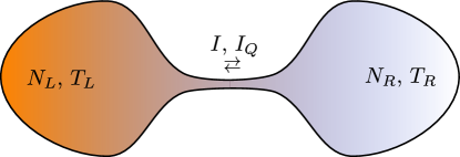
Figure 1: Two reservoirs of ultracold fermions connected via a tunnel junction allowing particle and heat transport. Each reservoir is characterized by the particle number $N$ and temperature $T$.

The Hamiltonian describing this system is assumed to be

$$H=H_{L}+H_{R}+H_{t}\>,$$ (1)

where $H_{L}$ and $H_{R}$ are the BCS Hamiltonians for the two reservoirs

$$H_{L} =\sum_{p\sigma}\xi_{p}c^{\dagger}_{p\sigma}c_{p\sigma}+\frac{1}{2}\sum_{pp^{\prime}\sigma}V_{pp^{\prime}}c^{\dagger}_{p\sigma}c^{\dagger}_{-p-\sigma}c_{-p^{\prime}-\sigma}c_{p^{\prime}\sigma}\>,$$ (2)

$$H_{R} =\sum_{k\sigma}\xi_{k}a^{\dagger}_{k\sigma}a_{k\sigma}+\frac{1}{2}\sum_{kk^{\prime}\sigma}V_{kk^{\prime}}a^{\dagger}_{k\sigma}a^{\dagger}_{-k-\sigma}a_{-k^{\prime}-\sigma}a_{k^{\prime}\sigma}\>.$$

Here, $c_{p\sigma}$ and $c^{\dagger}_{p\sigma}$ ($a_{p\sigma}$ and $a^{\dagger}_{p\sigma}$) are the annihilation (creation) operators of a fermion with momentum $p$ and spin $\sigma$ in the left (right) reservoir, $\xi_{p}=\varepsilon_{p}-\mu$ is the single-particle energy with respect to the chemical potential, and $V_{pp^{\prime}}$ is the (singlet) pairing interaction. In the context of neutral fermionic atoms the spin degree of freedom is represented by the two hyperfine states of the atom in consideration. The tunneling Hamiltonian is

$$H_{t}=\sum_{kp\sigma}\eta_{kp}a^{\dagger}_{k\sigma}c_{p\sigma}+h.c.\>,$$ (3)

where $\eta_{kp}$ is the tunneling matrix element, which in the following we assume to be energy independent, $|\eta_{kp}|^{2}=|\eta|^{2}$.

In the next step, we restrict ourselves to the mean-field approximation for the Hamiltonians in Eq. (2) introducing the mean-field parameter $\Delta_{L}$ for the left reservoir

$$\Delta_{p\sigma-\sigma}=-\sum_{p^{\prime}}V_{pp^{\prime}}\left<c_{-p^{\prime}-\sigma}c_{p^{\prime}\sigma}\right>\approx\Delta_{L}$$ (4)

and analogously for the right reservoir.

In a dilute gas of neutral fermionic atoms it is a good approximation to describe the interaction $V_{pp^{\prime}}$ between two atoms using a single parameter, the s-wave scattering length $a$. Consequently, the dimensionless interaction parameter $(k_{F}a)^{-1}$ can be included in the BCS gap equation using a standard renormalization procedure (see, e.g. Appendix 8A of Ref. Leggett2006, ). The gap equation then takes the form

$$\frac{\pi}{k_{F}a}\sqrt{\varepsilon_{F}}=\int_{0}^{\infty}\mathrm{d}\varepsilon\sqrt{\varepsilon}\left[\frac{1}{\varepsilon}-\frac{1}{E}\tanh\left(\frac{E}{2T}\right)\right],$$ (5)

where $E=\sqrt{(\varepsilon-\mu)^{2}+|\Delta|^{2}}$ and $\varepsilon_{F}$ is the Fermi energy. In Eq. (5), there are two unknown variables $\mu$ and $\Delta$. To solve it, the second equation is obtained by fixing the number of particles

$$\frac{4}{3}\varepsilon_{F}^{3/2}=\int_{0}^{\infty}\mathrm{d}\varepsilon\sqrt{\varepsilon}\left[1-\frac{\varepsilon-\mu}{E}\tanh\left(\frac{E}{2T}\right)\right].$$ (6)

For the density of states (DOS) of a 3D Fermi gas in the normal state $\mathcal{N}^{0}(\varepsilon)\propto\sqrt{\varepsilon}$ (neglecting the confining potential) which we used above, the integrals in Eqs. (5) and (6) converge and no cut-off energy needs to be introduced. The solution to these equations is shown in Fig. 2 as a function of temperature $T$ and interaction parameter $(k_{F}a)^{-1}$. As the interaction parameter approaches the BCS limit, $(k_{F}a)^{-1}\ll-1$, the superconducting gap $\Delta$ and critical temperature $T_{c}$ are proportional to $e^{-\pi/(2k_{F}a)}$ and $\mu/\varepsilon_{F}\to 1$ at $T=0$ Leggett2006 . On the other hand, towards unitarity, where $(k_{F}a)^{-1}\to 0^{-}$, $\Delta$ and $T_{c}$ increase and $\mu$ decreases.

Note that this mean-field critical temperature $T_{c}$ is in fact the pairing temperature below which a significant number of fermions are bound in pairs. In the BCS limit the real critical temperature and mean-field $T_{c}$ coincide, however, closer to the unitary regime, this approximation starts to fail.

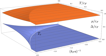
Figure 2: Solution for $\Delta$ (blue) and $\mu$ (orange) following from Eqs. (5) and (6) as a function of $(k_{F}a)^{-1}$ and $T$. The mean-field critical temperature $T_{c}$ is shown as a white curve. In the BCS limit $(k_{F}a)^{-1}\to-\infty$, the chemical potential $\mu/\varepsilon_{F}\to 1$ and $\Delta$ as well as $T_{c}$ approach zero.

An initial state with particle number imbalance or temperature imbalance between the left and right reservoirs will give rise to particle and heat transport. The particle current $I$ and energy current $I_{\mathcal{E}}$ are defined as

$$I =-\frac{\partial\langle\hat{N}_{L}\rangle}{\partial t}=i\langle[\hat{N}_{L},H]\rangle$$ (7)

$$I_{\mathcal{E}} =-\frac{\partial\langle H_{L}\rangle}{\partial t}=i\langle[H_{L},H]\rangle\>,$$

where the angular brackets represent the thermodynamic average in the grandcanonical ensemble and $\hat{N}_{L}=\sum_{p\sigma}c^{\dagger}_{p\sigma}c_{p\sigma}$ is the fermion number operator in the left reservoir. All the operators are in the Heisenberg picture.

If we restrict ourselves to quasiparticle transport (ignoring Cooper pairs and interference terms between Cooper pairs and quasiparticles), the expressions for the particle and heat current in the tunneling limit read

$$I =I_{L\to R}-I_{R\to L}$$ (8)

$$=\frac{2\pi|\eta|^{2}}{\hbar}\mathcal{V}_{L}\mathcal{V}_{R}\int_{-\infty}^{\infty}\mathrm{d}E\mathcal{N}_{L}(E)\mathcal{N}_{R}(E)\left[f_{L}(E)-f_{R}(E)\right]$$

and

$$I_{Q} =I_{Q,L\to R}-I_{Q,R\to L}$$

$$=\frac{2\pi|\eta|^{2}}{\hbar}\mathcal{V}_{L}\mathcal{V}_{R}\int_{-\infty}^{\infty}\mathrm{d}E\mathcal{N}_{L}(E)\mathcal{N}_{R}(E)$$

$$\times\left[(E-\mu_{L})f_{L}(E)(1-f_{R}(E))\right.$$

$$\left.-(E-\mu_{R})f_{R}(E)(1-f_{L}(E))\right]\>.$$ (9)

Here, $\mathcal{V}_{L(R)}$ is the volume and $f_{L(R)}(E)$ the Fermi function describing the left (right) reservoir. The superconducting density of states

$$\mathcal{N}_{L(R)}(E)=\text{Re}\,\{\mathcal{N}^{0}_{L(R)}(\varepsilon)\}\text{Re}\,\{\frac{|E-\mu_{L(R)}|}{\sqrt{(E-\mu_{L(R)})^{2}-\Delta^{2}_{L(R)}}}\}$$

contains the energy-dependent density of states $\mathcal{N}^{0}_{L(R)}$ of a normal 3-dimensional Fermi gas that can be expressed as

$$\mathcal{N}^{0}_{L(R)}(\varepsilon)=\frac{1}{2\pi^{2}}(\frac{2m}{\hbar^{2}})^{3/2}\sqrt{\varepsilon}=\frac{1}{2\pi^{2}}(\frac{2m}{\hbar^{2}})^{3/2}$$

$$\times\sqrt{\mu_{L(R)}+\text{sign}(E-\mu_{L(R)})\text{Re}\sqrt{(E-\mu_{L(R)})^{2}-\Delta^{2}_{L(R)}}}\>.$$

III Time evolution of the system

For finite reservoirs, which is the case we are studying here, a non-equilibrium initial state (like a temperature or particle number imbalance between the left and right reservoir) will induce time-dependent transport Bruderer2012 ; Grenier2012 ; Grenier2014 . To model this phenomenon we consider the balance equations for the particle number $N_{L(R)}$ and energy $\mathcal{E}_{L(R)}$ in each reservoir that lead to

$$\frac{\partial N_{L(R)}}{\partial t} =\mp I$$ (10)

$$\frac{\partial T_{L(R)}}{\partial t} =\mp\frac{1}{C_{\mathcal{V}_{L(R)}}}(I_{Q}+\mu_{L}I_{L\to R}-\mu_{R}I_{R\to L})\>.$$

Here, we used the relation between the energy of the left (right) reservoir and temperature change of the system at constant volume $C_{\mathcal{V}}=\partial\mathcal{E}/\partial T$. The heat capacity in the BCS theory is given by

$$C_{\mathcal{V}}(T) =\frac{2}{T}\int_{-\infty}^{\infty}\mathrm{d}E\mathcal{N}(E)\left(-\frac{\partial f(E)}{\partial E}\right)$$ (11)

$$\times\left(E^{2}-\frac{T}{2}\frac{\partial\Delta^{2}}{\partial T}+T\text{sign($E$)}\sqrt{E^{2}-\Delta^{2}}\frac{\partial\mu}{\partial T}\right)\>.$$

In writing Eqs. (10) and (11), we have neglected number and energy fluctuations in the reservoirs which were shown to be small in the regime considered here Schroll2007 .

To calculate the time evolution of the system, we proceed as follows: starting with $N_{L(R)}(t)=N\pm\delta N/2$ and $T_{L(R)}(t)=T\pm\delta T/2$ at time $t$, we calculate the corresponding values of $\mu_{L(R)}(t)$ and $\Delta_{L(R)}(t)$ using Eqs. (5) and (6). Then, using the discretized form of Eq. (10), we obtain $N_{L(R)}(t+\delta t)$ and $T_{L(R)}(t+\delta t)$ at time $t+\delta t$, and the procedure is iterated. The time evolution is hence uniquely determined by setting initial values of $N^{0}_{L(R)}$, $T^{0}_{L(R)}$ and $(k^{0}_{F,L}a)^{-1}$, where quantities with superscript $0$ denote the values at time $t=0$. The interaction parameter on the right side follows from $(k^{0}_{F,L}a)^{-1}$ and $N^{0}_{R}$. Note that in linear response in $\delta N$ and $\delta T$, assuming $\Delta_{L}=\Delta_{R}=0$ and $C_{\mathcal{V}}=$ constant, Eqs. (10) can be solved analytically using simple exponential functionsGrenier2012 . For example, an initial particle number imbalance will decay exponentially with time.

Typically, starting with an initial particle number (temperature) imbalance $\delta N_{0}$ ($\delta T_{0}$) will lead to a time-dependent temperature (particle number) imbalance due to the coupling between particle and heat transport. As a consequence, the chemical potential imbalance $\delta\mu=\mu_{L}-\mu_{R}$ and $\delta\Delta=\Delta_{L}-\Delta_{R}$ will also depend on time. Eventually, as $t\to\infty$, the system reaches an equilibrium state.

In the following we show and discuss three examples of such a time evolution displaying various quantities characterizing the system as a function of time. The time scale in Figs. 3–5 is fixed as follows: time can be expressed in units of $\varepsilon_{b}\hbar/|\eta|^{2}$, where $\varepsilon_{b}=\hbar^{2}/(2ma^{2})$ and $|\eta|^{2}=|\eta_{kp}|^{2}$ is the modulus squared of the tunneling matrix element introduced after Eq. (3). As mentioned earlier, the time evolution of a system in the normal state within linear response corresponds to an exponential decay of the initial particle number imbalance. To get an order-of-magnitude estimate for the absolute time scale in seconds, we compare our results for the dimensionless linear response coefficient $1/\tilde{\tau}$ in $\tilde{I}=\delta N/\tilde{\tau}$, where the tilde denotes dimensionless quantities, with the experimental value $1/\tau_{0}=2.9\,\mathrm{s}^{-1}$ taken from Ref. Brantut2012, . This leads to relation

$$\frac{\varepsilon_{b}\hbar}{|\eta|^{2}}=\tau_{0}/\tilde{\tau}.$$

The time scale $\tau_{0}$ represents a characteristic particle transport time scale and is analogous to the $RC$-time of a capacitor circuit.

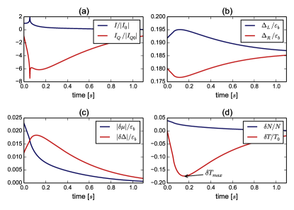
Figure 3: Time evolution of various quantities: (a) particle and heat current. (b) superconducting gap in the left and right reservoir. (c) chemical potential difference and difference between gaps in the left and right reservoir. (d) particle number difference and temperature difference. The sharp peak in the currents occurs for the time $t$ at which $|\delta\mu|=|\Delta_{L}-\Delta_{R}|$, i.e., when thermally excited quasiparticles are allowed to tunnel between the peaks in the DOS of the two reservoirs. The initial conditions chosen are $N=2\times 10^{4}$, $\delta N_{0}/N=0.04$, $T^{0}_{L}=T^{0}_{R}=T_{0}=0.07\varepsilon_{b}$, and $(k^{0}_{F,L}a)^{-1}=-1$.

Figure 3 demonstrates a case in which a sharp peak in the current as a function of time appears. This can be understood in the semiconductor picture of the tunneling process: the BCS DOS at the edges of the gap, $E=\pm\Delta$, in both reservoirs is divergent, provided that both reservoirs are in the superfluid regime. Hence, if the condition $|\delta\mu(t)|=|\Delta_{L}(t)-\Delta_{R}(t)|$ is satisfied, electrons from a peak in the DOS of one reservoir are allowed to tunnel into the peak in the DOS of the other reservoir. This condition creates a logarithmic singularity in the integrals in Eqs. (8), (II) (in the absence of gap anisotropy and level broadening) Tinkham2004 . Moreover, a time-dependent temperature imbalance $\delta T(t)$ develops that exhibits a non-monotonic behavior and reaches its maximum value $\delta T_{\text{max}}$ at a certain time, see Fig. 3(d). The build-up of this temperature imbalance is a signature of the Peltier effect. For the case shown in Fig. 3 the initial conditions are chosen such that both reservoirs are in the superfluid regime throughout the time evolution: $N=2\times 10^{4}$, $\delta N_{0}/N=0.04$, $T^{0}_{L}=T^{0}_{R}=T_{0}=0.07\,\varepsilon_{b}$, $(k^{0}_{F,L}a)^{-1}=-1$. The corresponding initial values of $T_{c}^{0}$ are $T_{c,L}^{0}=0.125\,\varepsilon_{b}$ and $T_{c,R}^{0}=0.119\,\varepsilon_{b}$.

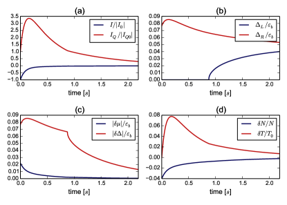
Figure 4: Time evolution of the same quantities as in Fig. 3. A negative initial particle number imbalance and an initial temperature between the transition temperatures of the two reservoirs leads to a transition of the left reservoir from an initially normal to a superfluid state at intermediate times. The initial conditions are $N=2\times 10^{4}$, $\delta N_{0}/N=-0.04$, $T^{0}_{L}=T^{0}_{R}=T_{0}=0.1248\,\varepsilon_{b}$, and $(k^{0}_{F,L}a)^{-1}=-1$.

In Fig. 4 we choose a negative initial particle number imbalance $\delta N_{0}/N=-0.04$ (while keeping $(k^{0}_{F,L}a)^{-1}=-1$) and an initial temperature $T^{0}_{L}=T^{0}_{R}=T_{0}=0.1248\,\varepsilon_{b}$ that lies between the initial transition temperatures of the two reservoirs. Since $T_{c,L}^{0}=0.119\,\varepsilon_{b}$ and $T_{c,R}^{0}=0.125\,\varepsilon_{b}$ in this case, the left reservoir is initially normal and the right one superfluid. During the time evolution, the left reservoir undergoes a transition to a superfluid state as shown in Fig. 4(b). Interestingly, this is not caused by lowering the temperature in the left reservoir. On the contrary, the temperature in the left reservoir actually temporarily rises. But the particle number (and hence the density) in the left reservoir rises which causes the transition from $\Delta_{L}=0$ to $\Delta_{L}\neq 0$. As before, the calculation was done for $N=2\times 10^{4}$.

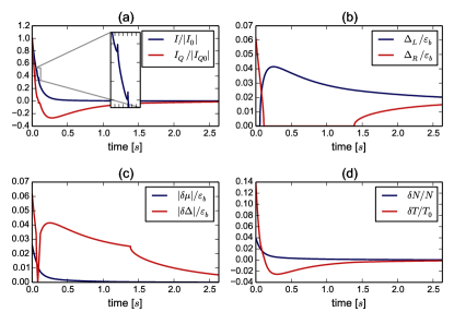
Figure 5: Time evolution of the same quantities as in Fig. 3. The system exhibits several transitions. The peaks in the particle and heat current are present for the same reason as in Fig. 3. In this case the condition $|\delta\mu|=\left|\Delta_{L}-\Delta_{R}\right|$ is satisfied twice during the time evolution. The initial conditions are $N=2\times 10^{4}$, $\delta N_{0}/N=0.04$, $T^{0}_{L}=0.132\,\varepsilon_{b}$, $T^{0}_{R}=0.115\,\varepsilon_{b}$, $T_{0}=(T^{0}_{L}+T^{0}_{R})/2$, and $(k^{0}_{F,L}a)^{-1}=-1$.

Figure 5 shows a more complex time evolution. The peaks in the current as a function of time appear for the same reason as in Fig. 3(a), but now the condition $|\delta\mu|=|\Delta_{L}(t)-\Delta_{R}(t)|$ is satisfied twice during the time-evolution, see Fig. 5(c). The system also undergoes several superfluid transitions similar to Fig. 4(b). Finally, when the system equilibrates for $t\to\infty$, both reservoirs end up in the superfluid state. The initial conditions were chosen as $N=2\times 10^{4}$, $\delta N_{0}/N=0.04$, $T^{0}_{L}=0.132\,\varepsilon_{b}$, $T^{0}_{R}=0.115\,\varepsilon_{b}$, $T_{0}=(T^{0}_{L}+T^{0}_{R})/2$, and $(k^{0}_{F,L}a)^{-1}=-1$.

As mentioned earlier, the induced temperature imbalance $\delta T$ due to an initial particle number imbalance $\delta N_{0}$ is a signature of the Peltier effect. It shows a non-monotonous behavior as a function of time with a maximum $\delta T_{\text{max}}$ at intermediate times, see Figs. 3(d) and 4(d). In Fig. 6 we show $|\delta T_{\text{max}}|$ as a function of $(k^{0}_{F,L}a)^{-1}$ for different values of the initial particle number imbalance $\delta N_{0}$ and initial temperature $T^{0}_{L}=T^{0}_{R}=T_{0}$. Each of the functions is divided into two sections monotonically increasing with increasing $(k^{0}_{F,L}a)^{-1}$. The left section represents data from a system which is in the normal state, $\Delta_{L(R)}(t)=0$, during the whole time evolution, whereas for the right section $\Delta_{L(R)}(t)\neq 0$, as in Fig. 3. Between the two sections, there is a “transient” regime, where superfluid transitions occur, similar to the ones in Figs. 4 and 5. The increase of $|\delta T_{\text{max}}|$ towards unitarity cannot be explained by particle-hole asymmetry alone but is due to a delicate interplay of the various factors in the integrands of Eqs. (8) and (II).

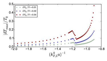
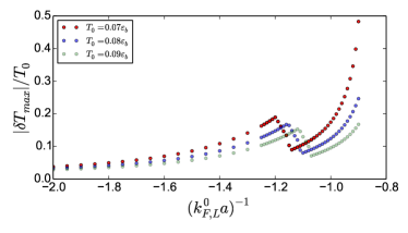
Figure 6: Maximal induced temperature imbalance $|\delta T_{\text{max}}|$ as a function of $(k_{F,L}^{0}a)^{-1}$ for different values of the initial particle number imbalance $\delta N_{0}$ and initial temperature $T^{0}_{L}=T^{0}_{R}=T_{0}$. Upper panel: $N=2\times 10^{4}$, $T_{0}=0.07\,\varepsilon_{b}$, and three different values of $\delta N_{0}/N$. Lower panel: $N=2\times 10^{4}$, $\delta N_{0}/N=0.04$, and three different values of $T_{0}$. The Peltier effect gets more significant approaching the unitary point.

IV Conclusion

To summarize, we have investigated particle and heat transport on the BCS side of the BCS-BEC crossover in a two-terminal setup with two reservoirs of interacting ultracold atoms. We have shown that a system initially out of equilibrium will show particle and/or thermal currents whose existence leads to characteristic time-dependent signatures, such as transitions between normal and superconducting states and resonant features in the currents as a function of time. An initial temperature imbalance can lead to a difference in chemical potentials at intermediate times. This is a signature of the Seebeck effect. Conversely, an initial particle number imbalance for two reservoirs at equal temperatures can lead to the build-up of a temperature difference at intermediate times, which is a signature of the Peltier effect. The maximal induced temperature imbalance increases if $(k_{F}a)^{-1}$ moves closer to the unitarity limit.

In conclusion, our paper points out a variety of dynamical features visible in the equilibration process that can be used to pin-point the parameters of the system. An experimental confirmation of the Peltier effect discussed here is important since an additional cooling mechanism for ultracold fermionic atoms will be a valuable resource. Furthermore, transport experiments in systems of ultracold atoms provide a fascinating laboratory in which the combination of particle and thermal currents can be explored in a regime that is not accessible to experiments with metallic superconductors.

- (1) A.A.M. Staring, L.W. Molenkamp, B.W. Alphenaar, H. van Houten, O.J.A. Buyk, M.A.A. Mabesoone, C.W.J. Beenakker, and C.T. Foxon, Europhys. Lett. 22, 57 (1993).
- (2) G.D. Guttman, E. Ben-Jacob, and D.J. Bergman, Phys. Rev. B 51, 17758 (1995).
- (3) F. Giazotto, T.T. Heikkilä, A. Luukanen, A.M. Savin, and J.P. Pekola, Rev. Mod. Phys. 78, 217 (2006).
- (4) P. Machon, M. Eschrig, and W. Belzig, Phys. Rev. Lett. 110, 047002 (2013).
- (5) A. Ozaeta, P. Virtanen, F.S. Bergeret, and T.T. Heikkilä, Phys. Rev. Lett. 112, 057001 (2014).
- (6) S. Kolenda, M.J. Wolf, and D. Beckmann, Phys. Rev. Lett. 116, 097001 (2016).
- (7) B.T. Seaman, M. Krämer, D.Z. Anderson, and M.J. Holland, Phys. Rev. A 75, 023615 (2007).
- (8) R.A. Pepino, J. Cooper, D.Z. Anderson, and M.J. Holland, Phys. Rev. Lett. 103, 140405 (2009).
- (9) R.A. Pepino, J. Cooper, D. Meiser, D.Z. Anderson, and M.J. Holland, Phys. Rev. A 82, 013640 (2010).
- (10) A. Ivanov, G. Kordas, A. Komnik, and S. Wimberger, Eur. Phys. J. B 86, 345 (2013).
- (11) J.-P. Brantut, J. Meineke, D. Stadler, S. Krinner, and T. Esslinger, Science 337, 1069 (2012).
- (12) D. Stadler, S. Krinner, J. Meineke, J.-P. Brantut, and T. Esslinger, Nature 491, 736 (2012).
- (13) J.-P. Brantut, C. Grenier, J. Meineke, D. Stadler, S. Krinner, C. Kollath, T. Esslinger, and A. Georges, Science 342, 713 (2013).
- (14) S. Krinner, D. Stadler, D. Husmann, J.-P. Brantut, and T. Esslinger, Nature 517, 64 (2015).
- (15) D. Husmann, S. Uchino, S. Krinner, M. Lebrat, T. Giamarchi, T. Esslinger, and J.-P. Brantut, Science 350, 1498 (2015).
- (16) M. Bruderer and W. Belzig, Phys. Rev. A 85, 013623 (2012).
- (17) C. Grenier, C. Kollath, and A. Georges, Probing thermoelectric transport with cold atoms, arXiv:1209.3942
- (18) C. Grenier, A. Georges, and C. Kollath, Phys. Rev. Lett. 113, 200601 (2014).
- (19) C. Grenier, C. Kollath, and A. Georges, Thermoelectric transport and Peltier cooling of cold atomic gases, arXiv:1607.03641
- (20) A.J. Leggett, Quantum Liquids (Oxford University Press, Oxford, 2006).
- (21) W. Belzig, C. Schroll, and C. Bruder, Phys. Rev. A 75, 063611 (2007).
- (22) M. Tinkham, Introduction to Superconductivity (Dover Publications, New York, 2004).