Multi-Modal Dictionary Learning for Image Separation With Application In Art Investigation

Abstract

In support of art investigation, we propose a new source separation method that unmixes a single X-ray scan acquired from double-sided paintings. In this problem, the X-ray signals to be separated have similar morphological characteristics, which brings previous source separation methods to their limits. Our solution is to use photographs taken from the front- and back-side of the panel to drive the separation process. The crux of our approach relies on the coupling of the two imaging modalities (photographs and X-rays) using a novel coupled dictionary learning framework able to capture both common and disparate features across the modalities using parsimonious representations; the common component models features shared by the multi-modal images, whereas the innovation component captures modality-specific information. As such, our model enables the formulation of appropriately regularized convex optimization procedures that lead to the accurate separation of the X-rays. Our dictionary learning framework can be tailored both to a single- and a multi-scale framework, with the latter leading to a significant performance improvement. Moreover, to improve further on the visual quality of the separated images, we propose to train coupled dictionaries that ignore certain parts of the painting corresponding to craquelure. Experimentation on synthetic and real data—taken from digital acquisition of the Ghent Altarpiece (1432)—confirms the superiority of our method against the state-of-the-art morphological component analysis technique that uses either fixed or trained dictionaries to perform image separation.

I Introduction

Big data sets—produced by scientific experiments or projects—often contain heterogeneous data obtained by capturing a physical process or object using diverse sensing modalities [2]. The result is a rich set of signals, heterogeneous in nature but strongly correlated due to their being generated by a common underlying phenomenon. Multi-modal signal processing and analysis is thus gaining momentum in various research disciplines ranging from medical diagnosis [3] to remote sensing and computer vision [4]. In particular, the analysis of high-resolution multi-modal digital acquisitions of paintings in support of art scholarship has proved a challenging field of research. Examples include the numerical characterization of brushstrokes [5, 6] for the authentication or dating of paintings, canvas thread counting [7, 8, 9] with applications in art forensics, and the (semi-) automatic detection and digital inpainting of cracks [10, 11, 12].

The Lasting Support project has focused on the investigation of the Ghent Altarpiece (1432), also known as The Adoration of the Mystic Lamb, a polyptych on wood panel painted by Jan and Hubert van Eyck. One of the most admired and influential masterpieces in the history of art, it has given rise to many puzzling questions for art historians. Currently, the Ghent Altarpiece is undergoing a major conservation and restoration campaign that is planned to end in 2017. The panels of the masterpiece were documented with various imaging modalities, amongst which visual macrophotography, infrared macrophotography, infrared reflectography and X-radiography [12]. A massive visual data set (comprising over 2TB of data) has been compiled by capturing small areas of the polyptych separately and stitching the resulting image blocks into one image per panel [13].

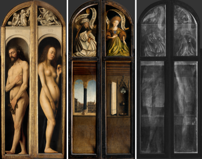
Figure 1: Panels from the Ghent Altarpiece: (left) panels of Adam and Eve, (centre) the respective paintings on the back, (right) corresponding X-ray images containing a mixture of components. ©KIK-IRPA

X-ray images are common tools in painting investigation, since they reveal information about the composition of the materials, the variations in paint thickness, the support as well as the cracks and losses in the ground and paint layers. The problem we address in this paper relates to the outer side panels, namely, the panels showing near life-sized depictions of Adam and Eve, shown in Fig. 1. Due to X-ray penetration, the scans of these panels are a mixture of the paintings from each side of the panel as well as the wood panel itself. The presence of all these components makes the reading of the X-ray image difficult for art experts, who would welcome an effective approach to separate the components.

The task of separating a mixture of signals into its constituent components is a popular field of research. Most work addresses the blind source separation (BSS) problem, where the goal is to retrieve the different sources from a given linear mixture. Several methods attempt to solve the BSS problem by imposing constraints on the sources’ structure. Independent component analysis (ICA) [14] commonly assumes that the components are independent non-Gaussian and attempts to separate them by minimizing the mutual information [15]. Nonnegative matrix factorization is another approach to solve the problem, where it is assumed that the sources are nonnegative (or they are transformed to a nonnegative representation) [16]. In an alternative path, the problem has been cast into a Bayesian framework, where either the sources are viewed as latent variables [17], or the problem is solved by maximizing the joint posterior density of the sources [18]. Under the Bayesian methodology, spatial smoothing priors (via, for example, Markov random fields) have been used to regularize blind image separation problems [19]. These assumptions do not fit our particular problem as both components have similar statistical properties and they are certainly not statistically independent.

Sparsity is another source prior heavily exploited in BSS [20, 21], as well as in various other inverse problems, such as, compressed sensing [22, 23], image inpainting [24, 25], denoising [26], and deconvolution [27]. Morphological component analysis (MCA), in particular, is a state-of-the-art sparsity-based regularization method, initially designed for the single-mixture problem [28, 20] and then extended to the multi-mixture case [29]. The crux of the method is the basic assumption that each component has its own characteristic morphology; namely, each has a highly sparse representation over a set of bases (or, dictionaries), while being highly non-sparse for the dictionaries of the other components. Prior work in digital painting analysis has employed MCA to remove cradling artifacts within X-ray images of paintings on a panel [30]. The cradling and painting components have very different morphologies, captured by different predefined dictionaries. Namely, complex wavelets [31] provide a sparse representation for the smooth X-ray image and shearlets [32] were used to represent the texture of the wood grain. Alternatively, dictionaries can be learned from a set of training signals; several algorithms have been proposed to construct dictionaries including the method of optimal directions (MOD) [33] and the K-SVD algorithm [34]. Both utilize the orthogonal matching pursuit (OMP) [35] method for sparse decomposition but they differ in the way they update the dictionary elements while learning. Recently, multi-mixture MCA has been combined with K-SVD, resulting in a method where dictionaries are learned adaptively while separating [36].

However, in our particular separation problem we have a simple mixture of two X-ray components that are morphologically very similar [see Fig. 1]. Hence, as we will show in the experimental section, simply using fixed or learned dictionaries is insufficient to discriminate one component from the other. Unlike prior work, in our setup we have access to high-quality photographic material from each side of the panel that can be used to assist the X-ray image separation process.

In this work, we elaborate on a novel method to perform separation of X-ray images from a single mixture by using images of another modality as side information. Our contributions are as follows:

• We present a new model based on parsimonious representations, which captures both the inherent similarities and the discrepancies among heterogeneous correlated data. The model decomposes the data into a sparse component that is common to the different modalities and a sparse component that uniquely describes each data type. Our model enables the formulation of appropriately regularized convex optimization procedures that address the separation problem at hand.

• We propose a novel dictionary learning approach that trains dictionaries coupling the images from the different modalities. Our approach introduces a new modified OMP algorithm that is tailored to our data model.

• We devise a novel method that ignores craquelure pixels—namely, pixels that visualize cracks in the surface of paintings—when learning coupled dictionaries. Paying no heed to these pixels avoids contaminating the dictionaries with high frequency noise, thereby leading to higher separation performance. Our approach bears similarities with inpainting approaches, e.g., [25]; it is, however, different in the way the dictionary learning problem is posed and solved.

• We devise a novel multi-scale image separation strategy that is based on a recursive decomposition of the mixed X-ray and visual images into low- and high-pass bands. As such, the method enables the accurate separation of high-resolution images even when a local sparsity prior is assumed. Our approach differs from existing multi-scale dictionary learning methods [37, 38, 25] not only by considering imaging data gleaned from diverse modalities but also in the way the multi-scale decomposition is constructed.

• We conduct experiments using synthetic and real data proving that the use of side information is crucial in the separation of X-ray images from double-sided paintings.

In the remainder of the paper: Section II reviews related work and Section III poses our source separation with side information problem. Section IV describes the proposed coupled dictionary learning algorithm. Section V presents our method that ignores cracks when learning dictionaries and, Section VI elaborates on our single- and multi-scale approaches to X-ray image separation. Section VII presents the evaluation of our algorithms while, Section VIII draws our conclusions.

II Related Work

II-A Source Separation

Adhering to a formal definition, MCA [28, 20] decomposes a source or image mixture $x=\sum_{i=1}^{\kappa}x_{i}$, with $x,x_{i}\in\mathbb{R}^{n\times 1}$, into its constituents, with the assumption that each $x_{i}$ admits a sparse decomposition in a different overcomplete dictionary $\Phi_{i}\in\mathbb{R}^{n\times d_{i}}$, $(n\ll\ d_{i})$. Namely, each component can be expressed as $x_{i}=\Phi_{i}z_{i}$, where $z_{i}\in\mathbb{R}^{d_{i}\times 1}$ is a sparse vector comprising a few non-zero coefficients: $\|z_{i}\|_{0}=\#\{\xi:z_{i_{\xi}}\neq 0,\xi=1,\dots,d_{i}\}=s_{i}\ll d_{i}$, with $\|\cdot\|_{0}$ denoting the $\ell_{0}$ pseudo-norm. The BSS problem is thus addressed as [28, 20]

$$(\hat{z}_{1},\dots,\hat{z}_{\kappa})=\arg\min_{z_{1},\dots,z_{\kappa}}\sum_{i=1}^{\kappa}\|z_{i}\|_{0}\;\;\text{s.t.}\;\;x=\sum_{i=1}^{\kappa}\Phi_{i}z_{i}.$$ (1)

Unlike the BSS problem, informed source separation (ISS) methods utilise some form of prior information to aid the task at hand. ISS methods are tailored to the application they address (to the best of our knowledge they are applied only for audio mixtures [39, 40]). For instance, an encoding/decoding framework is proposed in [39], where the sources are mixed at the encoder and the mixtures are sent to the decoder together with side information that is embedded by means of quantization index modulation (QIM) [41]. Unlike these methods, we propose a generic source separation framework that incorporates side information gleaned from a correlated heterogeneous source by means of a new dictionary learning method that couples the heterogenous sources.

II-B Dictionary Learning

Dictionary learning factorizes a matrix composed of training signals $X=[x_{1},\dots,x_{k}]\in\mathbb{R}^{n\times k}$ into the product $\Phi Z$ as

$$\Big{(}\Phi,Z\Big{)}=\arg\min_{\Phi^{\prime},Z^{\prime}}\|X-\Phi^{\prime}Z^{\prime}\|_{F}^{2}\;\;\text{s.t.}\;\|z_{i}\|_{0}\leq s,\;i=1,\dots,k,$$ (2)

where $Z=[z_{1},\dots,z_{k}]\in R^{d\times k}$ contains the sparse vectors corresponding to the signals $X=[x_{1},\dots,x_{k}]$ and $\|\cdot\|_{F}$ is the Frobenius norm of a matrix. The columns of the dictionary $\Phi$ are typically constrained to have unit norm so as to improve the identifiability of the dictionary. To solve Problem (2), which is non-convex, Olshausen and Field [42] proposed to iterate through a step that learns the sparse codes and a step that updates the dictionary elements. The same strategy is followed in subsequent studies [43, 33, 34, 44, 45]. Alternatively, polynomial-time algorithms that are guaranteed to reach a globally optimal solution appear in [46, 47].

In order to capture multi-scale traits in natural signals, a method to construct multi-scale dictionaries was presented in [25]. The multi-scale representation was obtained by using a quadtree decomposition of the learned dictionary. Alternatively, the work in [38, 37] applied dictionary learning in the domain of a fixed multi-scale operator (wavelets). In our approach we follow a different multi-scale strategy, based on a pyramid decomposition, similar to the Laplacian pyramid [48].

There exist dictionary learning approaches designed to couple multi-modal data. Monaci et al. [49] proposed an approach to learn basis functions representing audio-visual structures. The approach, however, enforces synchrony between the different modalities. Alternatively, Yang et al. [50, 51] considered the problem of learning two dictionaries $D_{x}$ and $D_{y}$ for two families of signals $x,y$, coupled by a mapping function $\mathcal{F}$ [with $y=\mathcal{F}(x)$]. The constraint was that the sparse representation of $x$ in $D_{x}$ is the same as that of $y$ in $D_{y}$. The application targeted was image super-resolution, where $x$ (resp. $y$) is the low (resp. high) resolution image. The study in [4] followed a similar approach with the difference that the mapping function was applied to the sparse codes, i.e., $z_{y}=\mathcal{F}(z_{x})$, rather than the signals. Jia et al. [52] proposed dictionary learning via the concept of group sparsity so as to couple the different views in human pose estimation. Our coupled dictionary learning method is designed to address the challenges of the targeted source separation application and as such, the model we consider to represent the correlated sources is fundamentally different from previous work. Moreover, we extend coupled dictionary learning to the multi-scale case and we provide a way to ignore certain noisy parts of the training signals (corresponding to cracks in our case).

III Image Separation with Side Information

We denote by $x^{\text{ray}}_{1}$ and $x^{\text{ray}}_{2}$ two vectorized X-ray image patches that we wish to separate from each other given a mixture patch $m$, where $m=x^{\text{ray}}_{1}+x^{\text{ray}}_{2}$. Let $y_{1}$ and $y_{2}$ be the co-located (visual) image patches of the front and back of the painting. These patches play the role of side information that aids the separation. The use of side information has proven beneficial in various inverse problems [53, 54, 55, 56, 57, 58, 59]. In this work, we consider the signals $x^{\text{ray}}_{1},x^{\text{ray}}_{2},y_{1},y_{2}\in\mathbb{R}^{n}$ to obey (superpositions of) sparse representations in some dictionaries:

$$y_{1} =\Psi^{c}z_{1c}$$

$$y_{2} =\Psi^{c}z_{2c},$$ (3)

and

$$x^{\text{ray}}_{1} =\Phi^{c}z_{1c}+\Phi v_{1}$$

$$x^{\text{ray}}_{2} =\Phi^{c}z_{2c}+\Phi v_{2},$$ (4)

where $z_{ic}\in\mathbb{R}^{\gamma\times 1}$, with $\|z_{ic}\|_{0}=s_{z}\ll\gamma$ and $i=1,2$, denotes the sparse component that is common to the images in the visible and the X-ray domain with respect to dictionaries $\Psi^{c},\Phi^{c}\in\mathbb{R}^{n\times\gamma}$, respectively. The parameter $s_{z}$ denotes the sparsity of the vector $z_{ic}$. Moreover, $v_{i}\in\mathbb{R}^{d\times 1}$, with $\|v_{i}\|_{0}=s_{v}\ll d$ denotes the sparse innovation component of the X-ray image, obtained with respect to the dictionary $\Phi\in\mathbb{R}^{n\times d}$. The common components express global features and structural characteristics that underlie both modalities. The innovation components capture parts of the signal specific to the X-ray modality, that is, traces of the wooden panel or even footprints of the vertical and horizontal wooden slats attached to the back the painting. We acknowledge the relation of our model with the sparse common component and innovations model that captures intra- and inter-signal correlation of physical signals in wireless sensor networks [56, 60]. Our approach is however more generic, since we decompose the signals in learnt dictionaries rather than fixed canonical bases, as in [60].

Given the proposed model and provided that the dictionaries $\Psi^{c}$, $\Phi$, and $\Phi^{c}$ are known, the corresponding X-ray separation problem can be formulated as

$$\begin{array}[]{ll}\underset{z_{1c},z_{2c},v_{1},v_{2}}{\text{minimize}}&\|z_{1c}\|_{1}+\|z_{2c}\|_{1}+\|v_{1}\|_{1}+\|v_{2}\|_{1}\\ \>\>\quad\text{s.t.}&m=\Phi^{c}z_{1c}+\Phi^{c}z_{2c}+\Phi v_{1}+\Phi v_{2}\\ &y_{1}=\Psi^{c}z_{1c}\\ &y_{2}=\Psi^{c}z_{2c}\end{array}$$ (9)

where we applied convex relaxation by replacing the $\ell_{0}$-pseudo norm with the $\ell_{1}$-norm, denoted as $\|\cdot\|_{1}$. Problem (9) is under-determined, namely, $v_{1}$ and $v_{2}$ cannot be distinguished due to the symmetry in the constraints. A solution to the unmixing problem can be obtained when $v_{1}=v_{2}=v$, which is formally written as

$$\begin{array}[]{ll}\underset{z_{1c},z_{2c},v}{\text{minimize}}&\|z_{1c}\|_{1}+\|z_{2c}\|_{1}+2\|v\|_{1}\\ \>\quad\text{s.t.}&m=\Phi^{c}z_{1c}+\Phi^{c}z_{2c}+2\Phi v\\ &y_{1}=\Psi^{c}z_{1c}\\ &y_{2}=\Psi^{c}z_{2c}\end{array}$$ (14)

Problem (14) boils down to basis pursuit, which is solved by convex optimization tools, e.g., [61]. The assumption $v_{1}=v_{2}$ is not only practical but is also motivated by the actual problem. Since the paintings are mounted on the same wooden panel, the sparse components that decompose the X-ray images via the dictionary $\Phi$ are expected to be the same.

IV Coupled Dictionary Learning Algorithm

In order to address the source separation with side information problem, we learn coupled dictionaries, $\Psi^{c}$, $\Phi^{c}$, $\Phi$, by using image patches sampled from visual and X-ray images of single-sided panels, which do not suffer from superposition phenomena. The images were registered using the algorithm described in [62]. Let $Y=[y_{1},\dots,y_{t}],X=[x_{1},\dots,x_{t}]\in\mathbb{R}^{n\times t}$ represent a set of $t$ co-located vectorized visual and X-ray patches, each containing $\sqrt{n}\times\sqrt{n}$ pixels. As per our model in (III) and (III), the columns of $X$ and $Y$ are decomposed as

$$Y =\Psi^{c}Z$$ (15a)

$$X =\Phi^{c}Z+\Phi V\,,$$ (15b)

where we collect their common components into the columns of the matrix $Z=[z_{1},\dots,z_{t}]\in\mathbb{R}^{\gamma\times t}$ and their innovation components into the columns of $V=[v_{1},\dots,v_{t}]\in\mathbb{R}^{d\times{t}}$. We formulate the coupled dictionary learning problem as

$$\begin{array}[t]{cl}\underset{\begin{subarray}{\hfil\lx@intercol{\\ }}\Psi^{c},Z\\ \Phi^{c},\Phi,V\end{subarray}}{\text{minimize}}&\frac{1}{2}\big{\|}Y-\Psi^{c}Z\big{\|}_{F}^{2}+\frac{1}{2}\big{\|}X-\Phi^{c}Z-\Phi V\big{\|}_{F}^{2},\\ \text{s.t.}&\big{\|}z_{\tau}\big{\|}_{0}\leq s_{z},\vspace{0.2cm}\par\\ &\big{\|}v_{\tau}\big{\|}_{0}\leq s_{v},\quad\forall\tau=1,2,\dots,t.\end{array}$$ (16)

Similar to related work [34, 25, 38], we solve Problem (16) by alternating between a sparse-coding step and a dictionary update step. Particularly, given initial estimates for dictionaries $\Psi^{c}$, $\Phi$, and $\Phi^{c}$—in line with prior work [34] we use the overcomplete discrete cosine transform (DCT) for initialization—we iterate on $k$ between a sparse-coding step:

$$(Z^{k+1},V^{k+1}) =\begin{array}[t]{cl}\underset{Z,V}{\text{arg\;min}}&\frac{1}{2}\Bigg{\|}\begin{bmatrix}Y\\ X\end{bmatrix}-\begin{bmatrix}{\Psi^{c}}^{k}&0\\ {\Phi^{c}}^{k}&\Phi^{k}\end{bmatrix}\begin{bmatrix}Z\\ V\end{bmatrix}\vspace{0.2cm}\Bigg{\|}_{F}^{2},\\ \text{s.t.}&\big{\|}z_{\tau}\big{\|}_{0}\leq s_{z},\vspace{0.2cm}\\ &\big{\|}v_{\tau}\big{\|}_{0}\leq s_{v},\quad\forall\tau=1,2,\dots,t,\end{array}$$ (20)

which is performed to learn the sparse codes $Z,V$ having the dictionaries fixed, and a dictionary update step

$$({\Psi^{c}}^{k+1},{\Phi^{c}}^{k+1}, \Phi^{k+1})=$$

$$\arg\min_{\Psi^{c},\Phi^{c},\Phi}\frac{1}{2}\Bigg{\|}\begin{bmatrix}Y\\ X\end{bmatrix}-\begin{bmatrix}{\Psi^{c}}&0\\ {\Phi^{c}}&\Phi\end{bmatrix}\begin{bmatrix}Z^{k+1}\\ V^{k+1}\end{bmatrix}\vspace{0.2cm}\Bigg{\|}_{F}^{2}.$$ (21)

which updates the dictionaries given the calculated sparse codes. The algorithm iterates between these steps until no additional iteration reduces the value of the cost function below a chosen threshold, or until a predetermined number of iterations is reached. In what follows, we provide details regarding the solution of the problem at each stage.

Sparse-coding step. Problem (20) decomposes into $t$ problems, each of which can be solved in parallel:

$$(z_{\tau}^{k+1},v_{\tau}^{k+1}) =\begin{array}[t]{cl}\underset{z_{\tau},v_{\tau}}{\text{arg\;min}}&\frac{1}{2}\Bigg{\|}\begin{bmatrix}y_{\tau}\\ x_{\tau}\end{bmatrix}-\begin{bmatrix}{\Psi^{c}}^{k}&0\\ {\Phi^{c}}^{k}&\Phi^{k}\end{bmatrix}\begin{bmatrix}z_{\tau}\\ v_{\tau}\end{bmatrix}\vspace{0.2cm}\Bigg{\|}_{F}^{2},\\ \text{s.t.}&\big{\|}z_{\tau}\big{\|}_{0}\leq s_{z},\vspace{0.2cm}\\ &\big{\|}v_{\tau}\big{\|}_{0}\leq s_{v}.\end{array}$$ (25)

To address each of the $t$ problems in (25), we propose a greedy algorithm that constitutes a modification of the OMP method [see Algorithm 1]. Our method adapts OMP [35] to solve:

$$\begin{array}[]{cc}\underset{w}{\text{minimize}}&\|b-\Theta w\|_{2}^{2}\\ \text{s.t.}&\|w(\mathcal{I})\|_{0}\leq s_{z},\\ &\|w(\mathcal{J})\|_{0}\leq s_{v},\end{array}$$ (29)

where $w(\mathcal{I})$ [resp., $w(\mathcal{J})$] denotes the components of vector $w\in\mathbb{R}^{(\gamma+d)\times 1}$ indexed by the index set $\mathcal{I}$ (resp., $\mathcal{J}$), with $\mathcal{I}\cup\mathcal{J}=\{1,2,\dots,\gamma+d\}$, $\mathcal{I}\cap\mathcal{J}=\{\emptyset\}$. Each sub-problem in (25) translates to (29) by replacing: $b=\begin{bmatrix}y_{\tau}\\ x_{\tau}\end{bmatrix}$, $\Theta=\begin{bmatrix}{\Psi^{c}}^{k}&0\\ {\Phi^{c}}^{k}&\Phi^{k}\end{bmatrix}$, and $w=\begin{bmatrix}z_{\tau}\\ v_{\tau}\end{bmatrix}$.

Algorithm 1 Modified Orthogonal Matching Pursuit (mOMP)

1:

2:A vector $b\in\mathbb{R}^{(2n)\times 1}$

3:A matrix $\Theta\in\mathbb{R}^{(2n)\times{(\gamma+d)}}$,

4:The indices $\mathcal{I}$, $\mathcal{J}$, with $\mathcal{I}\cup\mathcal{J}=\{1,2,\dots,\gamma+d\}$, $\mathcal{I}\cap\mathcal{J}=\{\emptyset\}$

5:The sparsity levels $s_{z}$, $s_{v}$ of vectors $z$ and $v$, respectively.

6:

7:$w$ (approximate) solution of (29).

8:

9:

10:Initialize the residual $r_{0}=b$.

11:Set the total sparsity of vector $w$ as $s_{w}=s_{z}+s_{v}$.

12:Set the counters for the sparsity of $z$ and $v$ to $\ell_{z}=0$, $\ell_{v}=0$.

13:Initialize the set of non-zero elements of $w$ to $\Omega=\emptyset$.

14:

15:

16:for $i=1,2,\dots,s_{w}$ do

17:    Sort the indices $\zeta=\{1,2,\dots,\gamma+d\}$, corresponding to the $\theta_{\zeta}$ columns of $\Theta$, such that $|\langle r_{i-1},\theta_{\zeta}\rangle|$ are in descending order (where $\langle\alpha,\beta\rangle$ denotes the inner product of the vectors $\alpha,\beta$). Then, put the ordered indices in the vector $q_{i}$.

18:    Set $\mathcal{G}=\emptyset$ and auxiliary iterator $\texttt{iter}=0$.

19:    while $\mathcal{G}=\emptyset$ do

20:         iter=iter+1

21:         Find the index of the $\Theta$ matrix that corresponds to the value of iter: $\kappa=q_{i}[\texttt{iter}]$.

22:         if $\kappa\in\mathcal{I}$ AND $\ell_{z}<s_{z}$ then

23:             Set $\mathcal{G}=\kappa$ and increase: $\ell_{z}=\ell_{z}+1$.

24:         else

25:             if $\kappa\in\mathcal{J}$ AND $\ell_{v}<s_{v}$ then

26:                 Set $\mathcal{G}=\kappa$ and increase: $\ell_{v}=\ell_{v}+1$.

27:             end if

28:         end if

29:    end while

30:    Update the set of non-zero elements of $w$, i.e., $\Omega_{i}=\Omega_{i-1}\cup\leavevmode\nobreak\ \{\kappa\}$, and the matrix of chosen atoms: $\Theta_{i}=[\Theta_{i-1}\quad\theta_{\kappa}]$.

31:    Solve: $w_{i}=\arg\min_{w}\|b-\Theta_{i}w\|_{2}$.

32:    Calculate the new residual: $r_{i}=b-\Theta_{i}w_{i}$.

33:end for

Dictionary update step. Problem (21) can be written as

$$\begin{array}[t]{ll}\underset{\Psi^{c},\overline{\Phi}}{\text{minimize}}&\frac{1}{2}\Big{\|}Y-\Psi^{c}Z^{k+1}\Big{\|}_{F}^{2}+\frac{1}{2}\Big{\|}X-\overline{\Phi}\>\overline{V}^{k+1}\Big{\|}_{F}^{2},\end{array}$$ (30)

where $\overline{\Phi}=\begin{bmatrix}\Phi^{c}&\Phi\end{bmatrix}$ and $\overline{V}^{k+1}=\begin{bmatrix}Z^{k+1}\\ V^{k+1}\end{bmatrix}$. Problem (30) decouples into two (independent) problems, that is,

$$\begin{array}[t]{ll}\underset{\Psi^{c}}{\text{minimize}}&\frac{1}{2}\Big{\|}Y-\Psi^{c}Z^{k+1}\Big{\|}_{F}^{2}\end{array}$$ (31)

and

$$\begin{array}[t]{ll}\underset{\overline{\Phi}}{\text{minimize}}&\frac{1}{2}\Big{\|}X-\overline{\Phi}\>\overline{V}^{k+1}\Big{\|}_{F}^{2}.\end{array}$$ (32)

Provided that $Z^{k+1}$ and $\overline{V}^{k+1}$ are full row-rank, each of these problems has a closed-form solution, namely,

$${\Psi^{c}}^{k+1}=Y{Z^{k+1}}^{T}\Big{(}{Z^{k+1}}{Z^{k+1}}^{T}\Big{)}^{-1}$$

and

$$\overline{\Phi}^{k+1}=X{\overline{V}^{k+1}}^{T}\Big{(}{\overline{V}^{k+1}}{\overline{V}^{k+1}}^{T}\Big{)}^{-1}.$$

When $Z^{k+1}$ and $\overline{V}^{k+1}$ are rank-deficient, (31) and (32) have multiple solutions, from which we select the one with minimal Frobenius norm. This is done by taking a thin singular value decomposition of $Z^{k+1}=G_{z^{k+1}}\Sigma_{z^{k+1}}U_{z^{k+1}}^{T}$ and $\overline{V}^{k+1}=G_{\overline{v}^{k+1}}\Sigma_{\overline{v}^{k+1}}U_{\overline{v}^{k+1}}^{T}$, and calculating

$${\Psi^{c}}^{k+1}=YU_{z^{k+1}}\Sigma_{z^{k+1}}^{-1}G_{z^{k+1}}^{T}$$

and

$$\overline{\Phi}^{k+1}=XU_{\overline{v}^{k+1}}\Sigma_{\overline{v}^{k+1}}^{-1}G_{\overline{v}^{k+1}}^{T}.$$

V Weighted Coupled Dictionary Learning

Visual and X-ray images of paintings contain a high number of pixels that depict cracks. These are fine patterns of dense cracking formed within the materials. When taking into account these pixels, the learned dictionaries comprise atoms that correspond to high frequency components. As a consequence, the reconstructed images are contaminated by high frequency noise. In order to improve the separation performance, our objective is to obtain dictionaries that ignore pixels representing cracks. To identify such pixels, we generate binary masks identifying the location of cracks by applying our method in [10]. Each sampled image patch may contain a variable number of crack pixels, meaning that each column of the data matrix contains a different number of meaningful entries. To address this issue, we introduce a weighting scheme that adds a weight of 0 or 1 to the pixels that do or do not correspond to cracks, respectively. These crack-induced weights are included using a Hadamard product, namely, our model in (15) is modified to

$$Y\odot\Lambda =(\Psi^{c}Z)\odot\Lambda$$ (33a)

$$X\odot\Lambda =(\Phi^{c}Z+\Phi V)\odot\Lambda.$$ (33b)

where the matrix $\Lambda$ has exactly the same dimensions as $X$ and $Y$ and its entries are 0 or 1 depending on whether a pixel is part of a crack or not, respectively. We now formulate the weighted coupled dictionary learning problem as

$$\begin{array}[t]{cl}\underset{\begin{subarray}{\hfil\lx@intercol{\\ }}\Psi^{c},Z\\ \Phi^{c},\Phi,V\end{subarray}}{\text{minimize}}&\frac{1}{2}\big{\|}(Y-\Psi^{c}Z)\odot\Lambda\big{\|}_{F}^{2}\\ &\qquad\qquad\qquad+\frac{1}{2}\big{\|}(X-\Phi^{c}Z-\Phi V)\odot\Lambda\big{\|}_{F}^{2},\\ \text{s.t.}&\big{\|}z_{\tau}\big{\|}_{0}\leq s_{z},\vspace{0.2cm}\par\\ &\big{\|}v_{\tau}\big{\|}_{0}\leq s_{v},\quad\forall\tau=1,2,\dots t.\end{array}$$ (34)

Similar to (16), the solution for (34) is obtained by alternating between a sparse-coding and a dictionary update step.

Sparse-coding step. Similar to (25), the sparse-coding problem decomposes into $t$ problems that can be solved in parallel:

$$(z_{\tau}^{k+1},v_{\tau}^{k+1})= \underset{z_{\tau},v_{\tau}}{\text{arg\;min}}\,\,\,\frac{1}{2}\Bigg{\|}\begin{bmatrix}y_{\tau}\\ x_{\tau}\end{bmatrix}\odot\begin{bmatrix}\lambda_{\tau}\\ \lambda_{\tau}\end{bmatrix}$$

$$\qquad-\Big{(}\begin{bmatrix}{\Psi^{c}}^{k}&0\\ {\Phi^{c}}^{k}&\Phi^{k}\end{bmatrix}\odot\Big{(}\begin{bmatrix}\lambda_{\tau}\\ \lambda_{\tau}\end{bmatrix}\boldsymbol{1}^{T}\Big{)}\Big{)}\begin{bmatrix}z_{\tau}\\ v_{\tau}\end{bmatrix}\Bigg{\|}_{2}^{2}$$

$$\quad\text{s.t.}\ \>\|z_{\tau}\|_{0}\leq s_{z},$$

$$\qquad\>\>\>\|v_{\tau}\|_{0}\leq s_{v},\quad\forall\tau=1,2,\dots t,$$ (35)

where we used $\lambda_{\tau}$ to represent column $\tau$ of $\Lambda$ and $\boldsymbol{1}^{T}$ to denote a row-vector of ones with dimension equal to $\gamma+d$. To address each of the $t$ sub-problems in (V), we use the mOMP algorithm described in Algorithm 1, as each sub-problem in (V) reduces to (29) by replacing: $b=\begin{bmatrix}y_{\tau}\\ x_{\tau}\end{bmatrix}\odot\begin{bmatrix}\lambda_{\tau}\\ \lambda_{\tau}\end{bmatrix}$, $\Theta=\begin{bmatrix}{\Psi^{c}}^{k}&0\\ {\Phi^{c}}^{k}&\Phi^{k}\end{bmatrix}\odot\Big{(}\begin{bmatrix}\lambda_{\tau}\\ \lambda_{\tau}\end{bmatrix}\boldsymbol{1}^{T}\Big{)}$, and $w=\begin{bmatrix}z_{\tau}\\ v_{\tau}\end{bmatrix}$.

Dictionary update step. The dictionary update problem is now written as

$$\begin{array}[t]{ll}\underset{\Psi^{c},\overline{\Phi}}{\text{minimize}}&\frac{1}{2}\Big{\|}Y\odot\Lambda-(\Psi^{c}Z^{k+1})\odot\Lambda\Big{\|}_{F}^{2}\\ &\qquad\quad+\frac{1}{2}\Big{\|}X\odot\Lambda-(\overline{\Phi}\>\overline{V}^{k+1})\odot\Lambda\Big{\|}_{F}^{2},\end{array}$$ (36)

and it decouples into:

$$\underset{\Psi^{c}}{\text{minimize}}\frac{1}{2}\Big{\|}Y\odot\Lambda-(\Psi^{c}Z^{k+1})\odot\Lambda\Big{\|}_{F}^{2}$$ (37a)

$$\underset{\overline{\Phi}}{\text{minimize}}\frac{1}{2}\Big{\|}X\odot\Lambda-(\overline{\Phi}\>\overline{V}^{k+1})\odot\Lambda\Big{\|}_{F}^{2}.$$ (37b)

We present only the solution of the first problem since the solution of the other follows the same logic. Specifically, we express the Frobenius norm in (37a) as the sum of $t$ $\ell_{2}$-norm terms, each corresponding to a vectorized training patch

$$\sum_{\tau=1}^{t}\|y_{\tau}\odot\lambda_{\tau}-({\Psi^{c}}z_{\tau})\odot\lambda_{\tau}\|_{2}^{2}.$$ (38)

By replacing the Hadamard product with multiplication with a diagonal matrix $\Delta_{\tau}=\text{diag}(\lambda_{\tau})$, (38) can be written as

$$\sum_{\tau=1}^{t}\|\Delta_{\tau}y_{\tau}-\Delta_{\tau}{\Psi^{c}}z_{\tau}\|_{2}^{2}.$$ (39)

To minimize the expression in (39), we take the derivative with respect to the dictionary ${\Psi^{c}}$ and set it to zero:

$$\frac{\partial}{\partial\Psi^{c}}\sum_{\tau=1}^{t}\|\Delta_{\tau}y_{\tau}-\Delta_{\tau}{\Psi^{c}}z_{\tau}\|_{2}^{2}=0$$

$$\Longrightarrow \sum_{\tau=1}^{t}\frac{\partial}{\partial\Psi^{c}}\Big{[}(\Delta_{\tau}y_{\tau}-\Delta_{\tau}{\Psi^{c}}z_{\tau})^{T}(\Delta_{\tau}y_{\tau}-\Delta_{\tau}{\Psi^{c}}z_{\tau})\Big{]}=0$$

$$\Longrightarrow 2\sum_{\tau=1}^{t}\frac{\partial}{\partial\Psi^{c}}y_{\tau}^{T}\Delta_{\tau}^{T}\Delta_{\tau}{\Psi^{c}}z_{\tau}=\sum_{\tau=1}^{t}\frac{\partial}{\partial\Psi^{c}}z_{\tau}^{T}{{\Psi^{c}}}^{T}\Delta_{\tau}^{T}\Delta_{\tau}{\Psi^{c}}z_{\tau}$$

$$\Longrightarrow \sum_{\tau=1}^{t}\Big{(}\Delta_{\tau}^{T}\Delta_{\tau}y_{\tau}\boldsymbol{1}^{T}\Big{)}\odot(\boldsymbol{1}z_{\tau}^{T})$$

$$\qquad=\sum_{\tau=1}^{t}\Big{(}{{\Psi^{c}}}z_{\tau}z_{\tau}^{T}\Big{)}\odot((\lambda_{\tau}\odot\lambda_{\tau})\boldsymbol{1}^{T}).$$ (40)

Before proceeding with the method to solve (40), we recall that the entries of $\lambda_{\tau}$ are either 0 or 1. To avoid dividing by zero when solving (40), we have to update the rows of the dictionary matrix one-by-one. Specifically, for each row $i$ of ${\Psi^{c}}$, we consider the matrix $A_{i}=\sum_{\tau\in S_{i}}z_{\tau}z_{\tau}^{T}$, where $S_{i}$ is the support of the $i$-th row of $\Lambda$, and $z_{\tau}$ is the $\tau$-th column of $Z$. We also create a vector $c_{i}=\sum_{\tau\in S_{i}}Y(i,\tau)z_{\tau}$, where $Y(i,\tau)$ is the $(i,\tau)$-th entry of $Y$. Provided that $A_{i}$ is invertible, the $i$-th row of ${\Psi^{c}}$ (which we denote by the row-vector ${\psi^{c}_{i}}$) will be given by

$${\psi^{c}_{i}}=c_{i}A_{i}^{-1}.$$ (41)

If each $z_{\tau}$ is drawn randomly, $A_{i}$ is invertible with probability 1 whenever the cardinality of $S_{i}$ is at least equal to the number of columns of $\Psi_{c}$. Although in practice each $z_{\tau}$ is not randomly drawn, we still obtain an invertible $A_{i}$ by guaranteeing that the number of training samples is large enough.

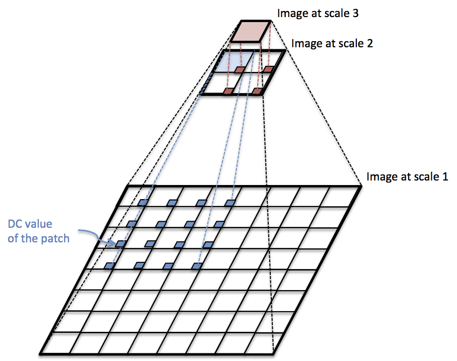
Figure 2: Schema of a 3-scale pyramid decomposition in the proposed multi-scale dictionary learning and source separation approaches.

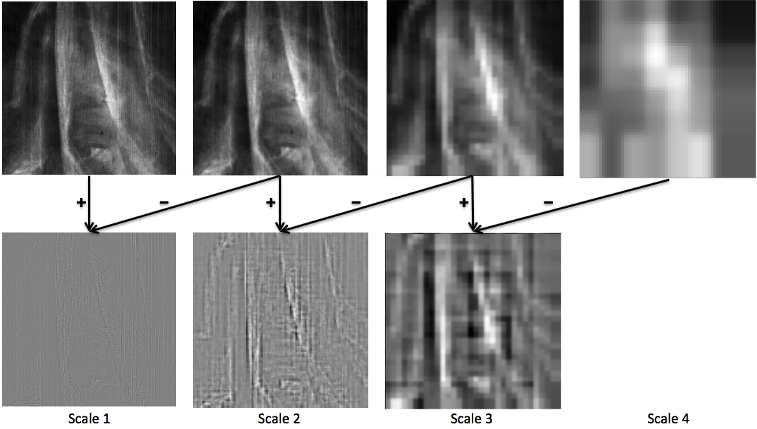
Figure 3: Example of a 4-scale pyramid decomposition of a mixed X-ray image. The original image resolution is $1024\times 1024$ pixels. At scale 1, the image is split into non-overlapping patches of $8\times 8$ pixels and the DC value of every patch is extracted, thereby generating the high-pass component. The aggregated DC values compose the low-pass component at scale 2, the resolution of which is $128\times 128$ pixels. Dividing this component into non-overlapping patches of $4\times 4$ pixels and extracting the DC value from every patch yields the high-pass band in scale 2. The procedure is repeated until finally the low-pass band at scale 4 has a resolution of $8\times 8$ pixels.

VI Single- And Multi-Scale Separation Methods

VI-A Single-Scale Approach

Given the trained coupled dictionaries, the source separation method described in Section III is applied locally, per overlapping patch of the X-ray image. Let the corresponding patches from the mixed X-ray and the two corresponding visual images be denoted as $m^{\boldsymbol{u}}$, $y_{1}^{\boldsymbol{u}}$, and $y_{2}^{\boldsymbol{u}}$, respectively. Each patch contains $\sqrt{n}\times\sqrt{n}$ pixels and has top-left coordinates

$$\boldsymbol{u}=(\epsilon\cdot u_{1},\epsilon\cdot u_{2}),\quad 0\leq u_{1}<\left\lfloor\frac{H}{\epsilon}\right\rfloor,\quad 1\leq u_{2}<\left\lfloor\frac{W}{\epsilon}\right\rfloor,$$

where $\epsilon\in\mathbb{Z}_{+}$, $1\leq\epsilon<\sqrt{n}$ is the overlap step-size, $\left\lfloor\bullet\right\rfloor$ is the floor function, and $H,W$ are the image height and width, respectively. Prior to separation, the DC value is removed from the pixels in each overlapping patch and the residual values are vectorized. The solution of Problem (14) yields the sparse components $z_{1c}^{\boldsymbol{u}},z_{2c}^{\boldsymbol{u}},\text{and}\ v^{\boldsymbol{u}}$ corresponding to the patch with coordinates $\boldsymbol{u}$. The texture of each separated patch is then reconstructed following the model in (III), that is, $x_{1}^{\boldsymbol{u}}=\Phi^{c}z_{1c}^{\boldsymbol{u}}+\Phi v^{\boldsymbol{u}}$ and $x_{2}^{\boldsymbol{u}}=\Phi^{c}z_{2c}^{\boldsymbol{u}}+\Phi v^{\boldsymbol{u}}$. In certain cases, the $v$ component may capture parts of the actual content; for example, vertical brush strokes can be misinterpreted as the wood texture of the panel. In this case, we can choose to skip the $v$ component; namely, we can reconstruct the texture of the X-ray patches as $x_{1}^{\boldsymbol{u}}=\Phi^{c}z_{1c}^{\boldsymbol{u}}$ and $x_{2}^{\boldsymbol{u}}=\Phi^{c}z_{2c}^{\boldsymbol{u}}$. The DC values are weighted according to the DC values of the co-located patches in the visual images and then added back to the corresponding separated X-ray patches. Finally, the pixels in each separated X-ray are recovered as the average of the co-located pixels in each overlapping patch.

VI-B Multi-Scale Approach

Due to the restricted patch size in comparison to the high resolution of the X-ray image, the DC values of all patches carry a considerable amount of the total image energy. In the single-scale approach, these DC values are common to the two separated X-rays, thereby leading to poor separation. To address this issue, we devise a multi-scale image separation approach. In contrast with the techniques in [37, 38, 25], the proposed multi-scale approach performs a pyramid decomposition of the mixed X-ray and visual images, that is, the images are recursively decomposed into low-pass and high-pass bands. The decompositions at scale $l=\{1,2,\dots,L\}$ are constructed as follows. The images at scale $l$—where we use the notation $M_{l},Y_{1,l},Y_{2,l}$, to refer to the mixed X-ray and the two visuals, respectively—are divided into overlapping patches $m_{l}^{\boldsymbol{u}_{l}},y_{1,l}^{\boldsymbol{u}_{l}},\>\text{and}\>y_{2,l}^{\boldsymbol{u}_{l}}$, each of size $\sqrt{n_{l}}\times\sqrt{n_{l}}$ pixels. Each patch has top-left coordinates

$$\boldsymbol{u}_{l}=(\epsilon_{l}\cdot u_{1,l},\epsilon_{l}\cdot u_{2,l}),\>0\leq u_{1,l}<\left\lfloor\frac{H_{l}}{\epsilon_{l}}\right\rfloor,\>0\leq u_{2,l}<\left\lfloor\frac{W_{l}}{\epsilon_{l}}\right\rfloor,$$

where $\epsilon_{l}\in\mathbb{Z}_{+},\>1\leq\epsilon_{l}<\sqrt{n_{l}}$ is the overlap step-size, and $H_{l},W_{l}$ are the height and width of the image decomposition at scale $l$. The DC value is extracted from each patch, thereby constructing the high frequency band of the image at scale $l$. The aggregated DC values comprise the low-pass component of the image, the resolution of which is $\left\lfloor\frac{H_{l}}{\epsilon_{l}}\right\rfloor\times\left\lfloor\frac{W_{l}}{\epsilon_{l}}\right\rfloor$ pixels. The low-pass component is then decomposed further at the subsequent scale ($l+1$). The pyramid decomposition is schematically sketched in Fig. 2 and exemplified in Fig. 3.

The texture of the mixed X-ray image at scale $l$ is separated patch-by-patch by solving Problem (14). The texture of each separated patch is then reconstructed as, $x_{1,l}^{\boldsymbol{u}_{l}}=\Phi^{c}_{l}z_{1c,l}^{\boldsymbol{u}_{l}}+\Phi_{l}v_{l}^{\boldsymbol{u}_{l}}$ and $x_{2,l}^{\boldsymbol{u}_{l}}=\Phi^{c}_{l}z_{2c,l}^{\boldsymbol{u}_{l}}+\Phi_{l}v_{l}^{\boldsymbol{u}_{l}}$; or alternatively, as $x_{1,l}^{\boldsymbol{u}_{l}}=\Phi^{c}_{l}z_{1c,l}^{\boldsymbol{u}_{l}}$ and $x_{2,l}^{\boldsymbol{u}_{l}}=\Phi_{l}^{c}z_{2c,l}^{\boldsymbol{u}_{l}}$. Note that the dictionary learning process can be applied per scale, yielding a triple of coupled dictionaries $(\Psi^{c}_{l},\Phi^{c}_{l},\Phi_{l})$ per scale $l$. In practice, due to lack of training data in the higher scales, dictionaries are learned only from the low-scale decompositions and then copied to the higher scales.

The separated X-ray images are finally reconstructed by following the reverse operation: descending the pyramid, the separated component at the coarser scale is up-sampled and added to the separated component of the finer scales.

VII Experiments

VII-A Experiments with Synthetic Data

As in [33, 34], we first evaluate the performance of our coupled dictionary learning algorithm—described in Section IV—and our source separation with side information method (see Section III) using synthetic data. Firstly, we generate synthetic signals, $x$, $y$, according to model (III), (III), using random dictionaries and then, given the data, we assess whether the algorithm recovers the original dictionaries. The random dictionaries $\Psi^{c}$, $\Phi$, and $\Phi^{c}$ of size $40\times{60}$ contain entries drawn from the standard normal distribution and their columns are normalized to have unit $\ell_{2}$-norm. Given the dictionaries, $t=1500$ sparse vectors $Z$ and $V$ were produced, each with dimension $\gamma=d=60$. The column-vectors $z_{\tau}$ and $v_{\tau}$, $\tau=1,2,\dots,t$, comprised of respectively $s_{z}=2$ and $s_{v}=3$ non-zero coefficients distributed uniformly and placed in random and independent locations. Combining the dictionaries and the sparse vectors according to the model in (15) yields the correlated data signals $X$ and $Y$, to which white Gaussian noise with a varying signal-to-noise ratio (SNR) has been added.

Table I: Dictionary Identifiability of the Proposed Algorithm Based on Synthetic Data, Expressed in Terms of the Percentage of Retrieved Atoms for the Dictionaries in Model (15).

SNR [dB]	$\infty$	40	35	30	25	20	15
$\Psi^{c}$	96%	95.18%	95.38%	95.65%	95.20%	90.42%	12.53%
$\Phi^{c}$	96.78%	95.97%	96.53%	96.50%	95.48%	74.35%	0.27%
​​$\Phi$	92.95%	91.90%	91.73%	91.27%	91.50%	88.25%	3.07%

Table II: Reconstruction error of the proposed Source Separation With Side Information Method based on Synthetic Data.

SNR [dB]	$\infty$	40	35	30	25	20	15
$x_{1}$	$1.66\times 10^{-5}$	0.0094	0.0307	0.0734	0.1215	0.2125	0.5854
$x_{2}$	$1.43\times 10^{-5}$	0.0097	0.0222	0.0818	0.0857	0.2516	0.2781

(a) Visual

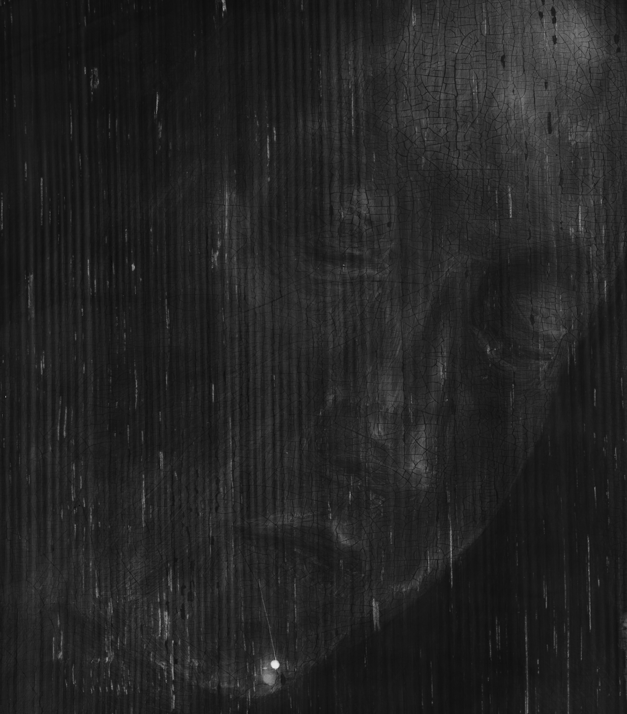
(b) X-ray ©KIK-IRPA

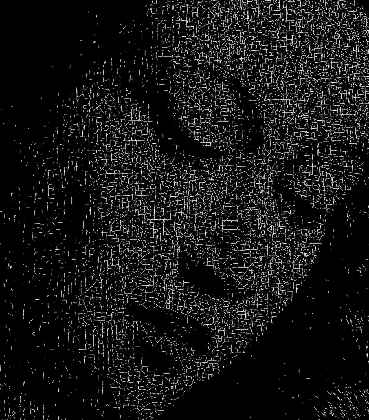
(c) Crack mask

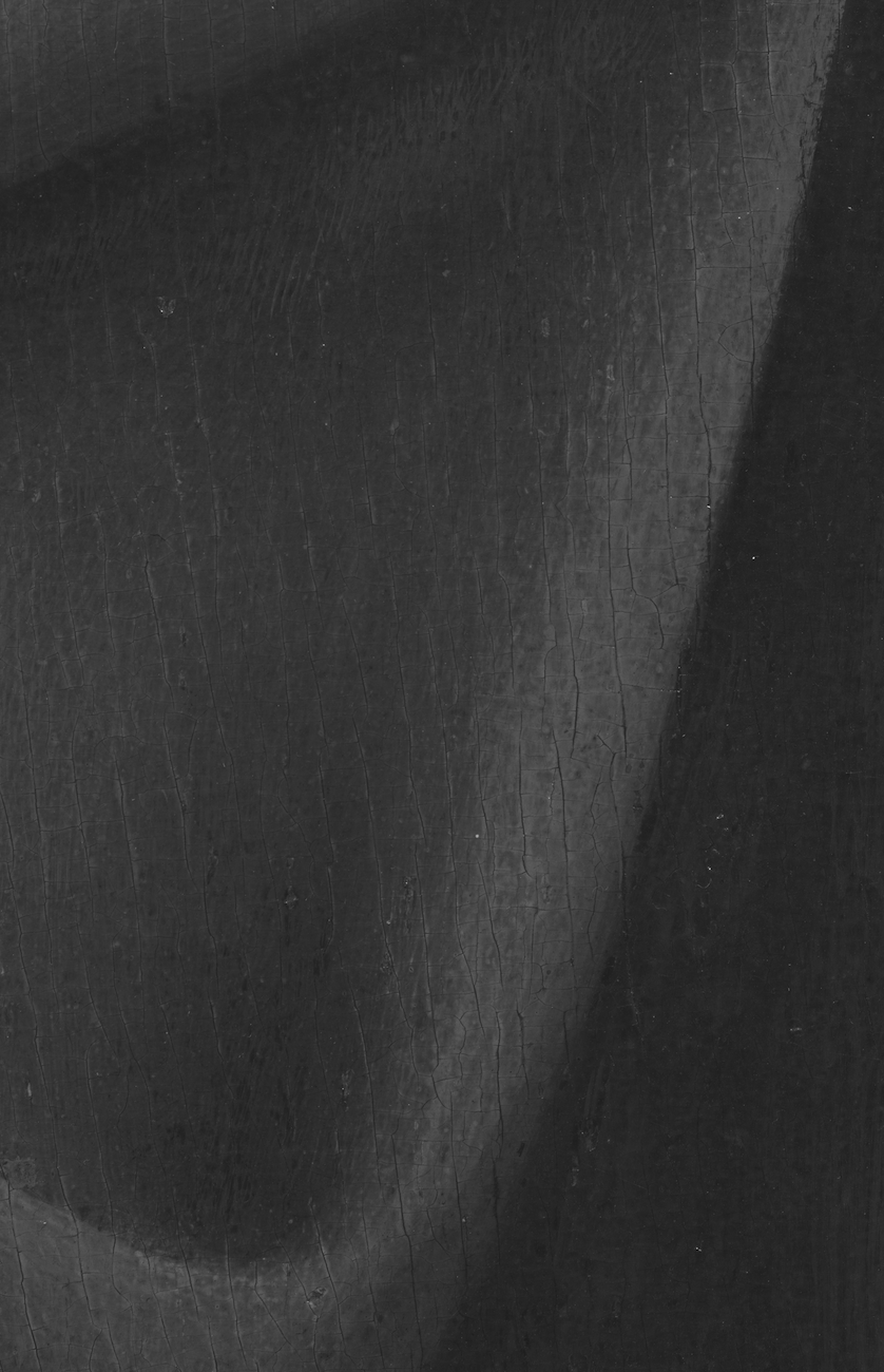
(d) Visual

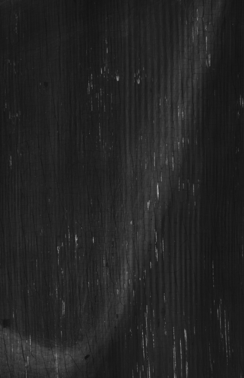
(e) X-ray ©KIK-IRPA

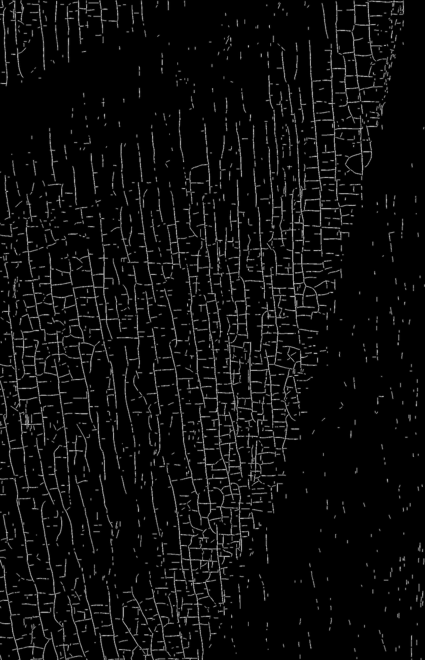
(f) Crack mask

Figure 4: Examples of images from single-sided panels of the Ghent Altarpiece and the corresponding crack masks.

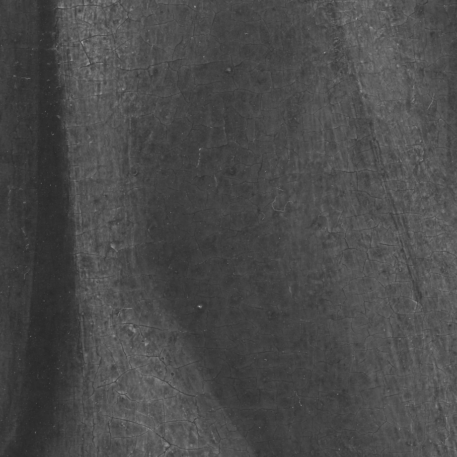
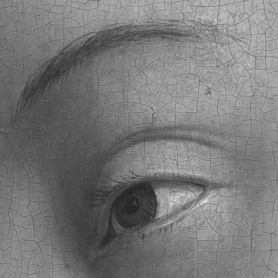
(a) ©KIK-IRPA

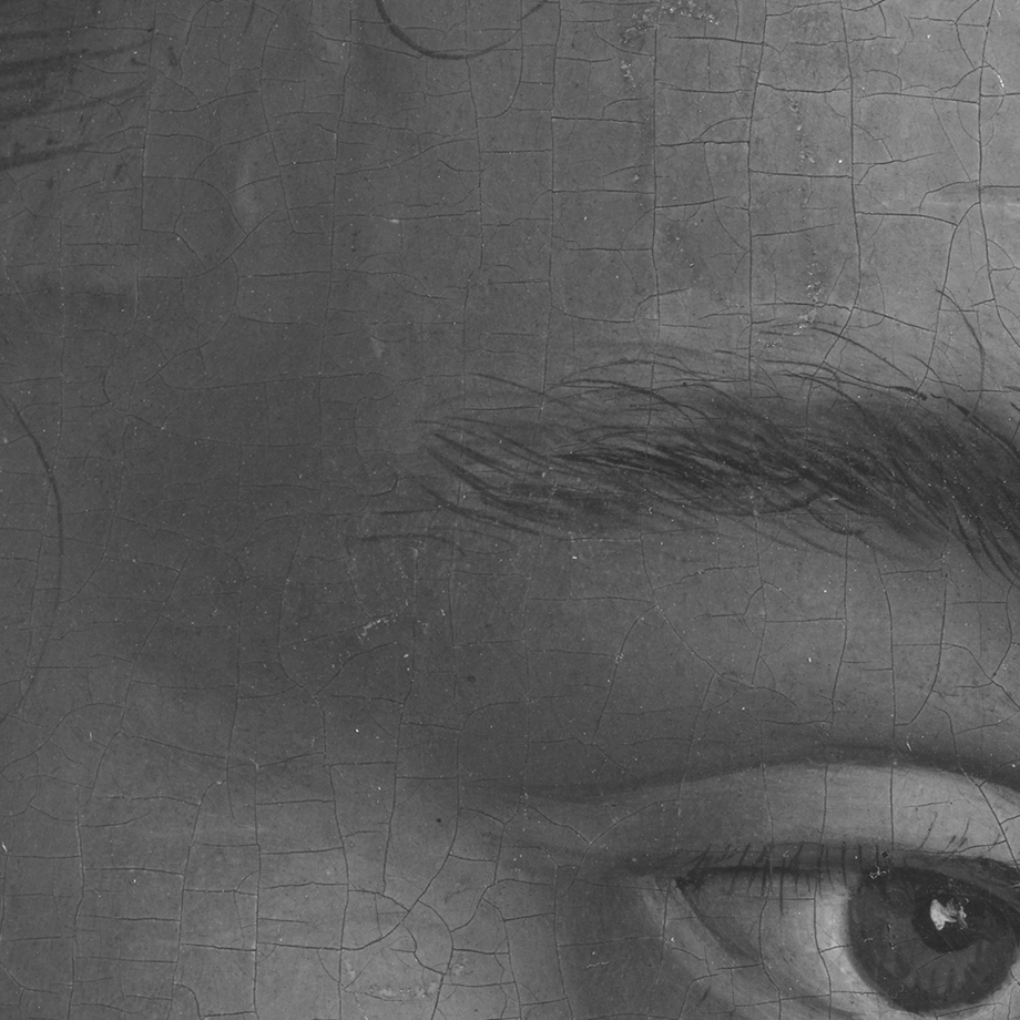
(b) ©KIK-IRPA

Figure 5: Image set cropped from a double-sided panel of the altarpiece, on which we assess the proposed method; (a) and (d) photograph of side 1, (b) and (e) photograph of side 2; (c) and (f) corresponding X-ray image. The resolution is $1024\times{1024}$ pixels.

To retrieve the initial dictionaries, we apply the proposed method in Section IV with the dictionaries initialised randomly and the maximum number of iterations set to 100—experimental evidence has shown that this value strikes a good balance between complexity and dictionary identifiability. To compare the retrieved dictionaries with the original ones, we adhere to the approach in [34]: per generating dictionary, we sweep through its columns and identify the closest column in the retrieved dictionary. The distance between the two columns is measured as $1-|\delta_{i}\tilde{\delta}^{T}_{j}|$, where $\delta_{i}$ is the $i$-th column in the original dictionary $\Psi^{c}$, $\Phi^{c}$, or $\Phi$, and $\tilde{\delta}_{j}$ is the $j$-th column in the corresponding recovered dictionary. Similar to [34], a distance less than 0.01 signifies a success. The percentage of successes per dictionary and for various SNR values is reported in Table I. The results, which are averaged over $100$ trials, show that for very noisy data (that is, $\text{SNR}\leq 15$) the dictionary identifiability performance is low. However, for SNR values higher than 20 dB, the percentage of recovered dictionary atoms is up to 96.78%. The obtained performance is systematic for different dictionary and signal sizes as well as for different sparsity levels.

In a second stage, given the learned dictionaries, we separate signal pairs $(x_{1},x_{2})$ from mixtures $m=x_{1}+x_{2}$ by solving Problem (14) using the corresponding pair $(y_{1},y_{2})$ as side information. The pairs are taken from the correlated data signals $X$ and $Y$, to which white Gaussian noise with a varying SNR has been added. Table II reports the normalized mean-squared error between the reconstructed—defined by $\tilde{x_{i}}$—and the original signals, that is, $\frac{\|x_{i}-\tilde{x_{i}}\|_{2}^{2}}{\|x_{i}\|_{2}^{2}}$, $i=\{1,2\}$. The results show that at low and moderate noise SNRs the reconstruction error is very low. When the noise increases, the recovery performance drops; this is to be expected as the noise affects both the dictionary leaning and the generation of the mixtures.

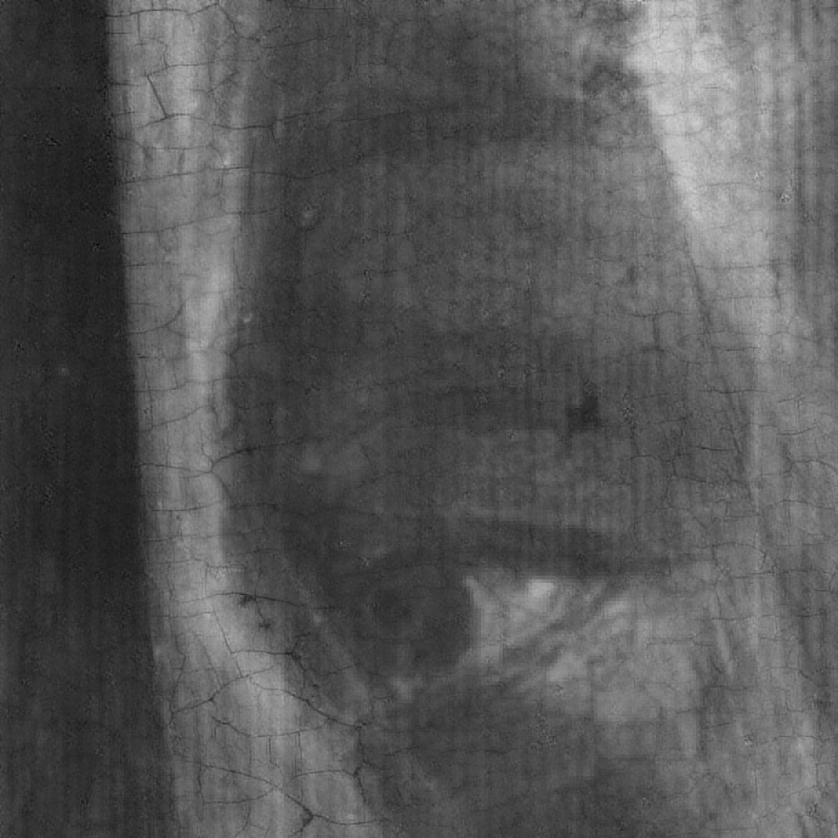
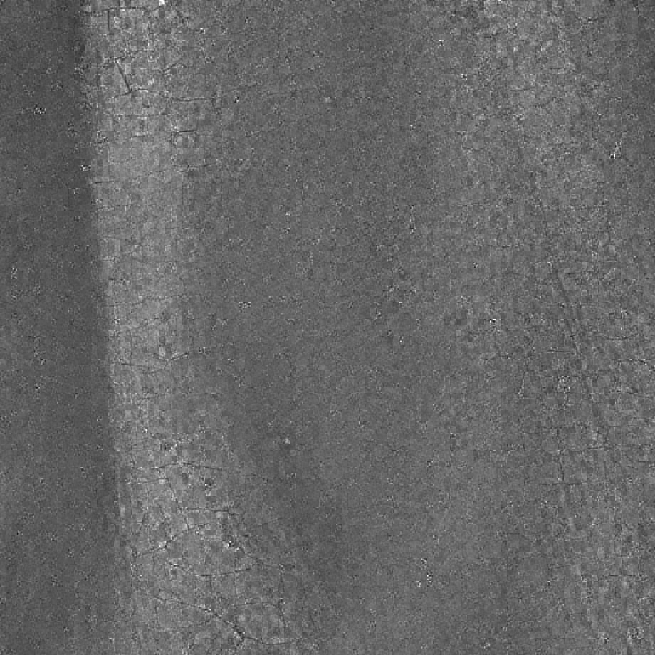
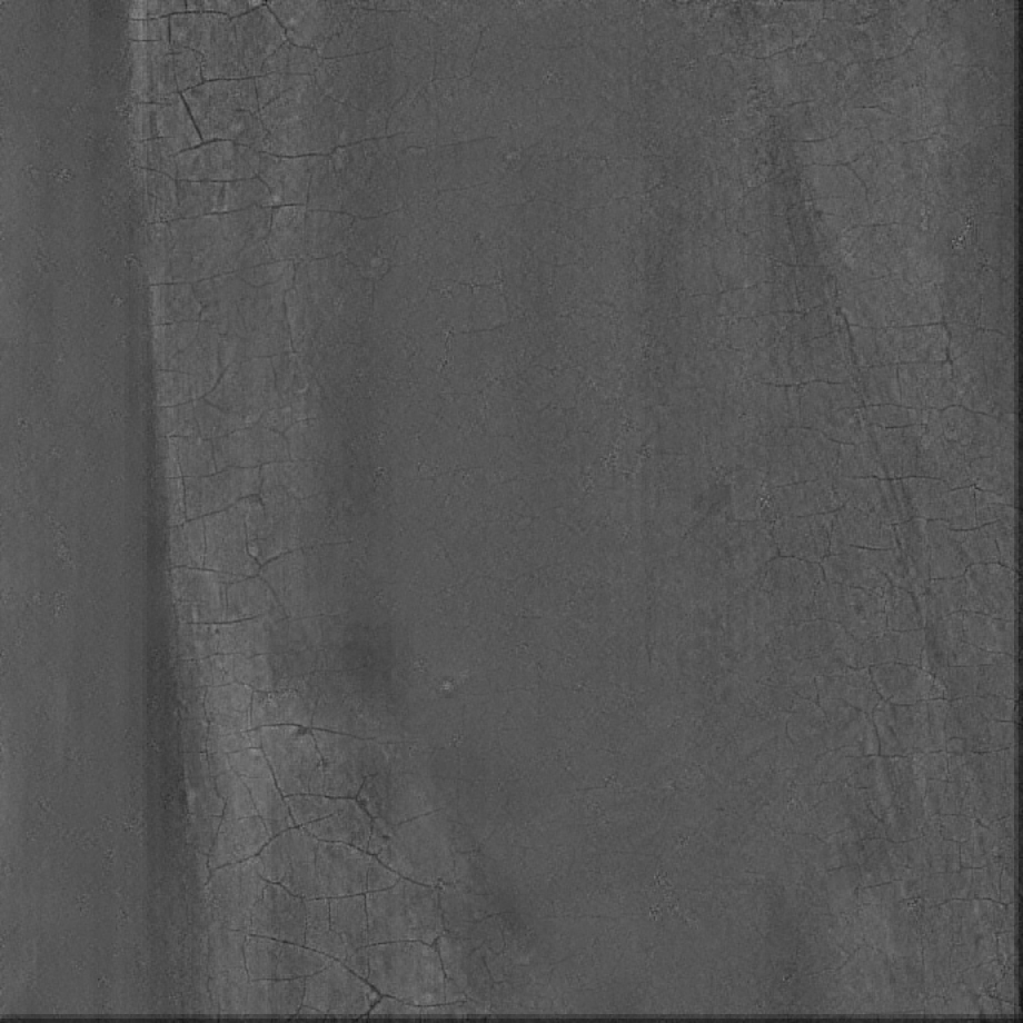
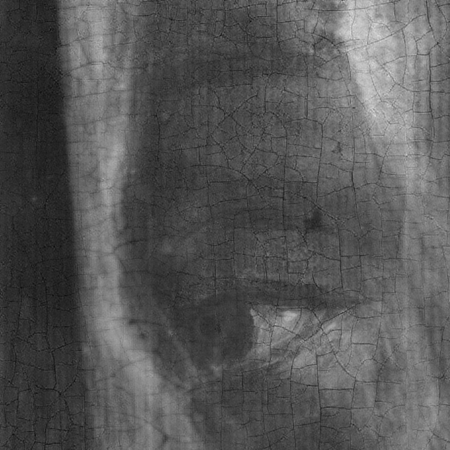
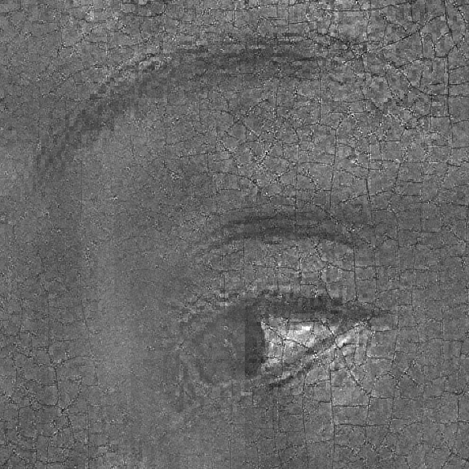
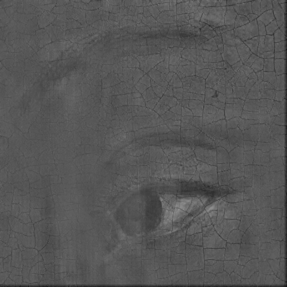
Figure 6: Visual evaluation of the different configurations of the proposed method in the separation of the X-ray image in Fig. 5(c); (first row) separated side 1, (second row) separated side 2. The configurations are: (first column) single-scale method (Section VI-A) with the coupled dictionary learning algorithm described in Section IV, (second column) multi-scale method (Section VI-B) with the coupled dictionary learning method from Section IV, (third column) multi-scale method (Section VI-B) with the weighted coupled dictionary learning method from Section V and without including the $v$ component.

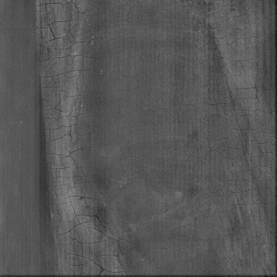
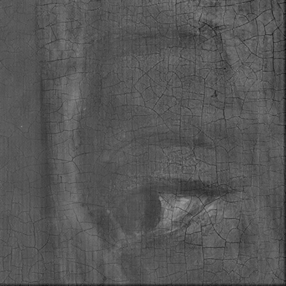
Figure 7: Visual evaluation of the proposed multi-scale method in the separation of the X-ray image in Fig. 5(c); (a) separated side 1, (b) separated side 2. The reconstructions include the X-ray specific $v$ component.

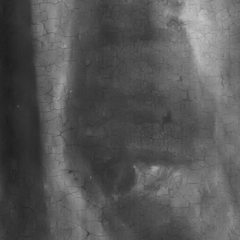
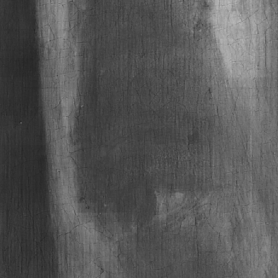
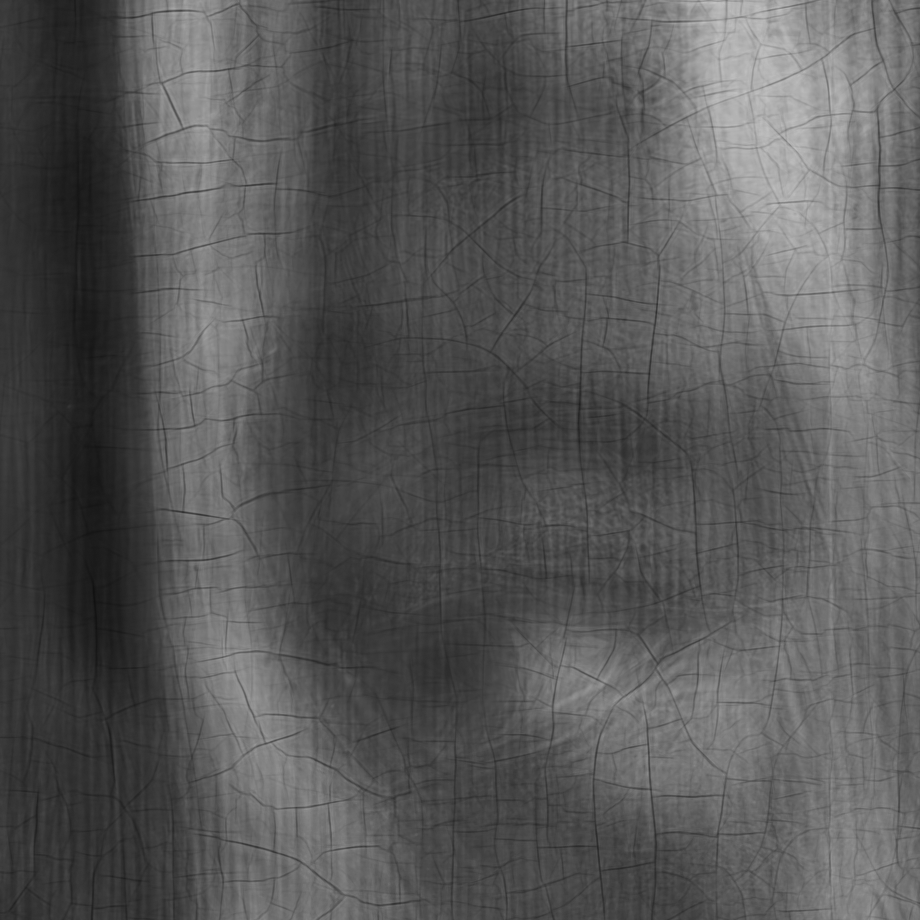
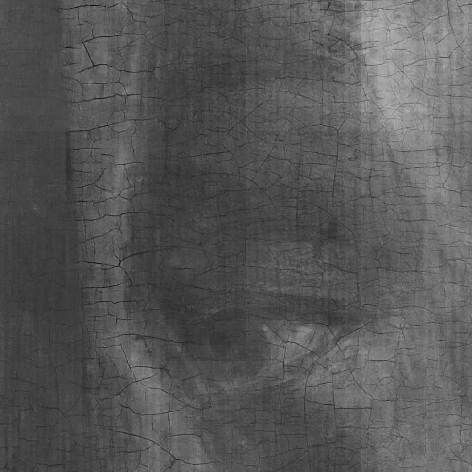
Figure 8: Visual evaluation of the proposed multi-scale method in the separation of the X-ray image in Fig. 5(c); (first row) separated side 1, (second row) separated side 2. The competing methods are: (first column) MCA with fixed dictionaries [30], (second column) multi-scale MCA with K-SVD, (third column) Proposed without including the $v$ component.

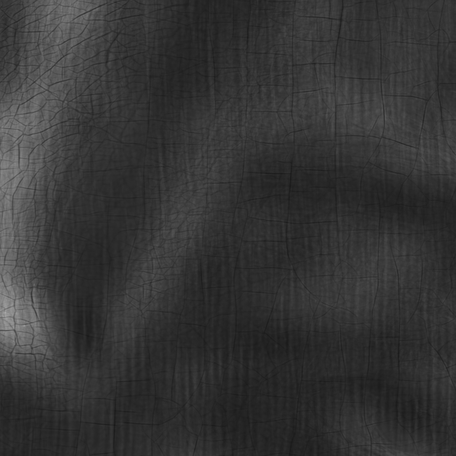
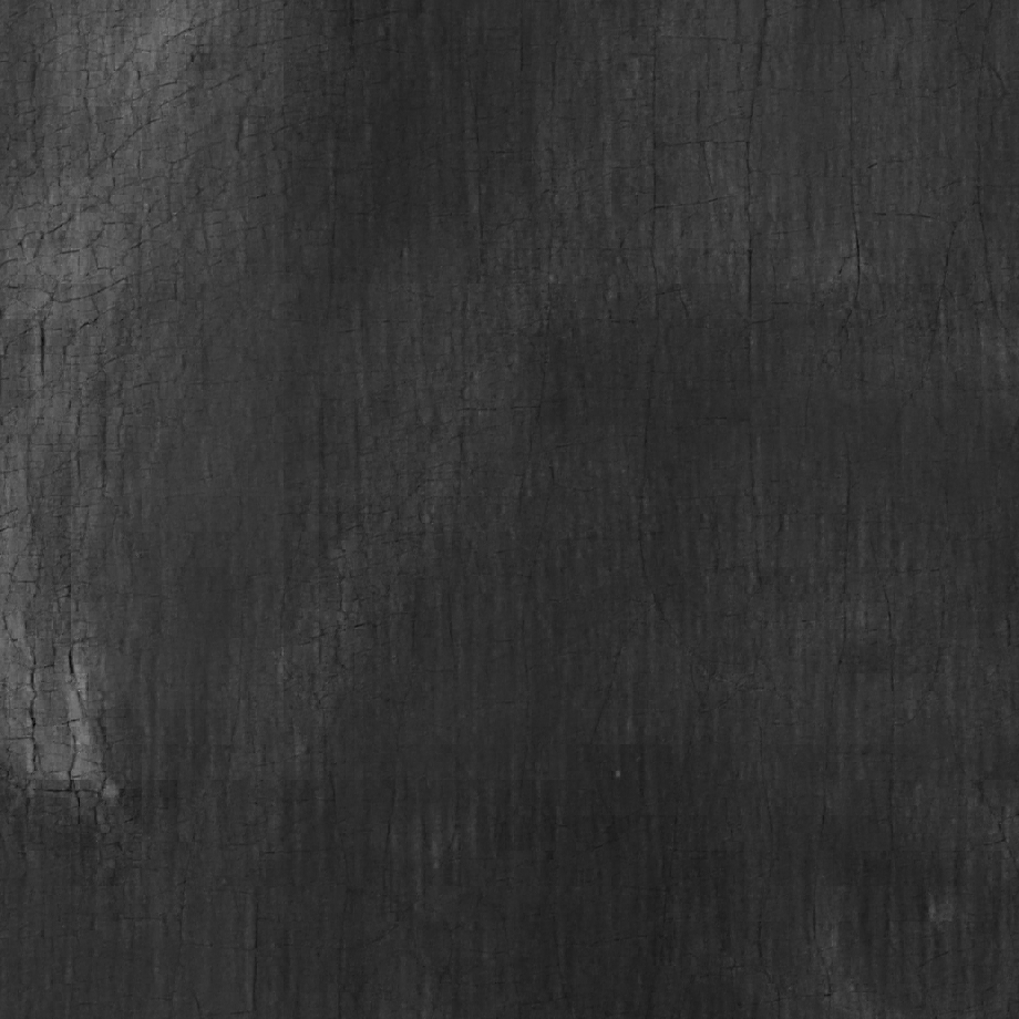
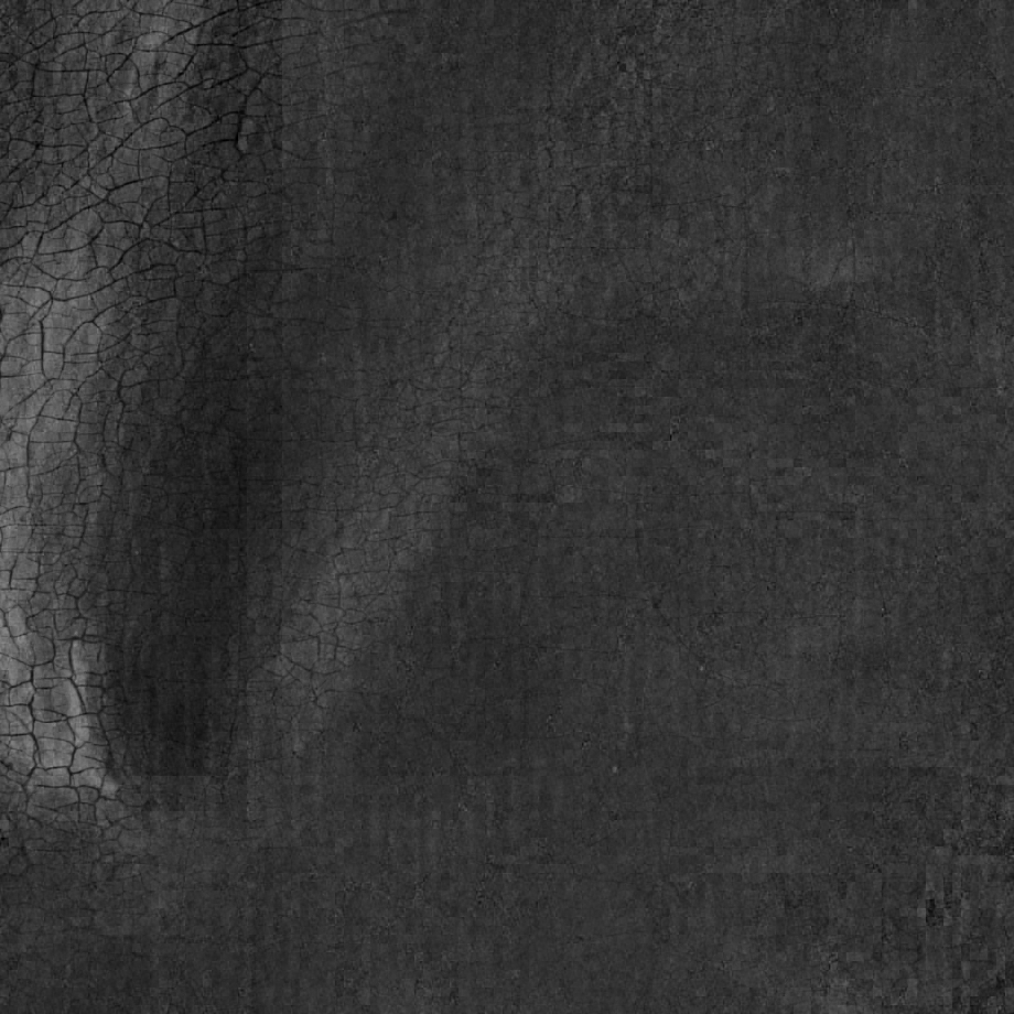
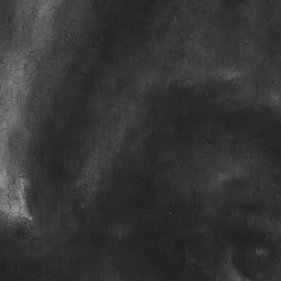
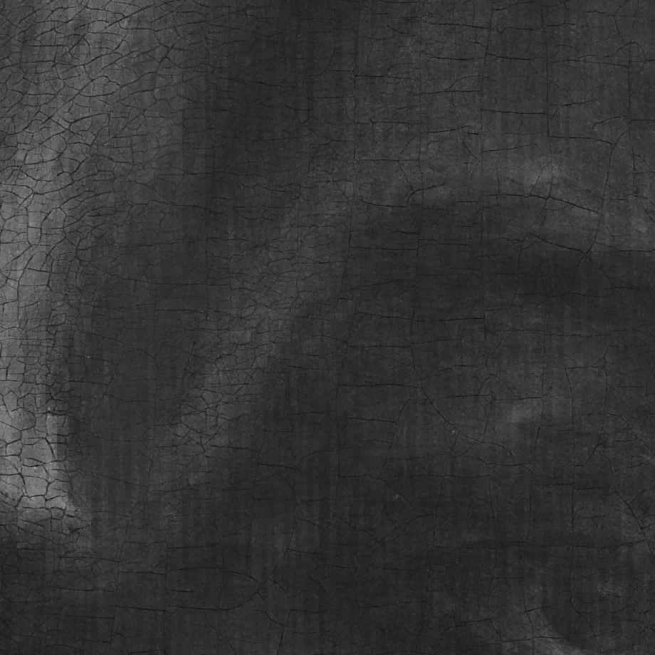
Figure 9: Visual evaluation of the proposed multi-scale method in the separation of the X-ray image in Fig. 5(f); (first row) separated side 1, (second row) separated side 2. The competing methods are: (first column) MCA with fixed dictionaries [30], (second column) multi-scale MCA with K-SVD, (third column) Proposed including the $v$ component.

VII-B Experiments with Real Data

We consider eight image pairs—each consisting of an X-ray scan and the corresponding photograph—taken from digital acquisitions [12] of single-sided panels of the Ghent Altarpiece (1432). Furthermore, we are given access to eight crack masks (one per visual/X-ray image pair) that indicate the pixel positions referring to cracks (these masks were obtained using our method in [10]). Fig. 4 depicts two such pairs with the crack masks, one visualizing a face and the other a piece of fabric. An example X-ray mixture (of size $1024\times 1024$ pixels) together with its two registered visual images corresponding to the two sides of the painting are depicted in Fig. 5.

Firstly, adhering to the single-scale approach, described in Section VI-A, we train a dictionary triplet, $(\Psi^{c},\Phi^{c},\Phi)$, using our method in Section IV. We use $t=46400$ patches, each containing $8\times{8}$ pixels, the dictionaries, $\Psi^{c}$, $\Phi^{c}$, $\Phi$, have a dimension of $64\times{256}$, and we set $s_{z}=10$ and $s_{v}=8$. The separated X-rays that correspond to the mixture in Fig. 5 are depicted in the first column of Fig. 6. We observe that our single-scale approach separates the texture of the X-rays; this is demonstrated by the accurate separation of the cracks. Still, however, the low-pass band content is not properly split over the images; namely, part of the cloth and the face are present in both separated images. Next, we apply the multi-scale framework, where we use $L=4$ scales with parameters $\sqrt{n_{l}}=8,\>l=\{1,2,3,4\}$, $\epsilon_{1}=4$, $\epsilon_{2}=4$, $\epsilon_{3}=7$, and $\epsilon_{4}=8$. Dictionary triplets $(\Psi^{c}_{\ell},\Phi^{c}_{\ell},\Phi_{\ell})$, each with dimension of $64\times{256}$, are trained for the first three scales and the dictionaries of the third scale are used for the forth. We use $t_{1}=46400$, $t_{2}=46400$ and $t_{3}=35500$ patches for scale 1, 2 and 3, respectively. The visualizations in the second column of Fig. 6 show that, compared to the single scale approach, the multi-scale method properly discriminates the low-pass frequency content of the two images (most part of the cloth is allocated to “Separated Side 1” while the face is only visible in “Separated Side 2”), thereby leading to a higher separation performance. Finally, we also construct dictionary triplets according to our weighted dictionary learning method in Section V. The remaining dictionary learning parameters are as before. It is worth mentioning that, in order to obtain a solution in (41), the number of training samples $t$ needs to be higher that the total dimension of the dictionary. Namely, to update the columns of dictionary $\Psi^{c}$ we need at least $16384$ samples. Correspondingly, to update the rows of dictionary $\overline{\Phi}$ we need more than $32768$ samples. The visual results in the third column of Fig. 6 corroborate that the quality of the separation is improved when the dictionaries are learned from only non-crack pixels. Indeed, with this configuration, the separated images are not only smoother but also the separation is more prominent.

It is worth mentioning that the results of our method, depicted in Fig. 6, are obtained without including the $v$ component during the reconstruction; namely, we reconstructed each X-ray patch as $x_{1}=\Phi^{c}z_{1c}$ and $x_{2}=\Phi^{c}z_{2c}$. The visual results of our method when including the $v$ component during the reconstruction are depicted in Fig. 7. These results are obtained with the same dictionaries that yield the result in the third column of Fig. 6. By comparing the two reconstructions, we can make the following observations. First, the $v$ component successfully expresses the X-ray specific features, such as the wood grain, visualized by the periodic vertical stripes in the X-ray scan. The reconstruction of these stripes is much more evident in Fig. 7. Secondly, in this case, the $v$ component also captures parts of the actual content that we wish to separate. For example, we can discern a faint outline of the eye in Fig. 7(a) as well as a fold of fabric appearing in Fig. 7(b).

We compare our best performing multi-scale approach (namely, the one that omits cracks when learning dictionaries) with the state-of-the-art MCA method [28, 20]. Two configurations of the latter are considered. Based on prior work [30], in one configuration we use fixed dictionaries, namely, the discrete wavelet and curvelet transforms are applied on blocks of $512\times 512$ pixels. Inherently, the low-frequency content cannot be split by MCA and it is equally divided between both retrieved components. In the other configuration, we learn dictionaries with K-SVD using the same training X-ray images as in the previous experiment. One dictionary is trained on the X-ray images depicting fabric and the other on the images of faces. The K-SVD parameters are the same as the ones used in our method. Furthermore, the same multi-scale strategy is applied to the configuration of MCA with K-SVD trained dictionaries. The results are depicted in Fig. 8 and Fig. 9. Note that the third column in Fig. 8 and Fig. 9 are without and with taking the $v$ component into account, respectively. It is clear that MCA with fixed dictionaries can only separate based on morphological properties; for example, the wood grain of the panel is captured entirely by curvelets and not by the wavelets. It is, however, unsuitable to separate painted content—it is evident that part of the cloth and face appear in both separated components. Furthermore, MCA with K-SVD dictionaries is also unable to separate the X-ray content. Nevertheless, we do observe that most cracks are captured by the face dictionary, as more cracks are present in that type of content. Unlike both state-of-the-art configurations of MCA, the proposed method separates the X-ray content accurately (the cloth is always depicted on “Separated Side 1” while the face is only visible in “Separated Side 2”), leading to better visual performance. These results corroborate the benefit of using side information by means of photographs to separate mixtures of X-ray images.

VII-C Experiments on Simulated Mixtures

Due to the lack of proper ground truth data, we generate simulated X-ray image mixtures in an attempt to assess our method in an objective manner. To this end, we utilised the X-ray images from single-sided panels, depicting content similar to the mixture in Fig. 5(c) and (f). We generated mixtures by summing these independent X-ray images and then we assessed the separation performance of the proposed method vis-à-vis MCA  either with fixed or K-SVD trained dictionaries. For this set of experiments, patches of size $256\times 256$ pixels were considered and the parameters of the different methods were kept the same as in the previous section. Table III reports the quality of the reconstructed X-ray components by means of the peak-signal-to-noise-ratio (PSNR) and structural similarity index metric (SSIM) [63]. It is clear that the proposed method outperforms the alternative state-of-the-art methods both in terms of PSNR and SSIM performance. Compared to MCA with fixed dictionaries, the proposed method brings an improvement in the quality of the separation by up to $1.26$dB in PSNR and $0.0741$ in SSIM for “Mixture 3”. The maximum gains against MCA with K-SVD trained dictionaries are $1.41$dB and $0.0953$ for “Mixture 3” again. While we realize that PSNR and SSIM are not necessarily the right image quality metrics in this scenario, they do demonstrate objectively the improvements that our method brings over the state of the art.

Table III: Objective Quality Assessment of the X-Ray Separation Performance of Different Methods on Simulated Mixtures.

		Mixture 1		Mixture 2		Mixture 3		Mixture 4		Mixture 5
	Image	PSNR [dB]	SSIM	PSNR [dB]	SSIM	PSNR [dB]	SSIM	PSNR [dB]	SSIM	PSNR [dB]	SSIM
MCA fixed	X-ray 1	25.69	0.7941	30.87	0.9003	27.28	0.7915	27.99	0.7972	26.96	0.8473
	X-ray 2	25.50	0.8134	30.73	0.8818	27.15	0.8198	27.86	0.8628	26.78	0.8068
MCA trained	X-ray 1	26.04	0.8245	31.07	0.8381	28.13	0.7703	27.56	0.7783	27.24	0.8258
	X-ray 2	25.83	0.8485	31.15	0.8189	27.23	0.6966	27.41	0.8464	27.05	0.7927
Proposed	X-ray 1	26.21	0.8583	31.91	0.9072	28.54	0.8656	28.31	0.8266	27.34	0.8592
	X-ray 2	26.00	0.8759	31.75	0.8892	28.36	0.8859	28.16	0.8921	27.14	0.8329

VIII Conclusion

We have proposed a novel sparsity-based regularization method for source separation guided by side information. Our method learns dictionaries, coupling registered acquisitions from diverse modalities, and comes both in a single- and multi-scale framework. The proposed method is applied in the separation of X-ray images of paintings on wooden panels that are painted on both sides, using the photographs of each side as side information. Experiments on real data, consisting of digital acquisitions of the Ghent Altarpiece (1432), verify that the use of side information can be highly beneficial in this application. Furthermore, due to the high resolution of the data relative to the restricted patch size, the multi-scale version of the proposed algorithm improves the quality of the results significantly. We also observed experimentally that omitting the high frequency crack pixels in the dictionary learning process results in smoother and visually more pleasant separation results. Finally, the superiority of our method, compared to the state-of-the-art MCA technique [20, 21, 36], was validated visually using real data and objectively using simulated X-ray image mixtures.

References

- [1] N. Deligiannis, J. F. C. Mota, B. Cornelis, M. R. D. Rodrigues, and I. Daubechies, “X-ray image separation via coupled dictionary learning,” in IEEE Int. Conf. Image Process. (ICIP). [Available: arXiv:1605.06474], 2016, pp. 1––5.
- [2] M. Chen, S. Mao, and Y. Liu, “Big data: A survey,” Mobile Networks and Applications, vol. 19, no. 2, pp. 171–209, 2014.
- [3] D. Zhang and D. Shen, “Multi-modal multi-task learning for joint prediction of multiple regression and classification variables in Alzheimer’s disease,” NeuroImage, vol. 59, no. 2, pp. 895–907, 2012.
- [4] S. Wang, L. Zhang, Y. Liang, and Q. Pan, “Semi-coupled dictionary learning with applications to image super-resolution and photo-sketch synthesis,” in IEEE Conference on Computer Vision and Pattern Recognition (CVPR), 2012, pp. 2216–2223.
- [5] C. R. Johnson, E. Hendriks, I. J. Berezhnoy, E. Brevdo, S. M. Hughes, I. Daubechies, J. Li, E. Postma, and J. Z. Wang, “Image processing for artist identification,” IEEE Signal Process. Mag., vol. 25, no. 4, pp. 37–48, 2008.
- [6] N. van Noord, E. Hendriks, and E. Postma, “Toward discovery of the artist’s style: Learning to recognize artists by their artworks,” IEEE Signal Process. Mag., vol. 32, no. 4, pp. 46–54, July 2015.
- [7] D. Johnson, C. Johnson Jr., A. Klein, W. Sethares, H. Lee, and E. Hendriks, “A thread counting algorithm for art forensics,” in IEEE Digital Signal Processing Workshop and IEEE Signal Processing Education Workshop (DSP/SPE), Jan 2009, pp. 679–684.
- [8] H. Yang, J. Lu, W. Brown, I. Daubechies, and L. Ying, “Quantitative canvas weave analysis using 2-D synchrosqueezed transforms: Application of time-frequency analysis to art investigation,” IEEE Signal Process. Mag., vol. 32, no. 4, pp. 55–63, July 2015.
- [9] L. van der Maaten and R. Erdmann, “Automatic thread-level canvas analysis: A machine-learning approach to analyzing the canvas of paintings,” IEEE Signal Process. Mag., vol. 32, no. 4, pp. 38–45, July 2015.
- [10] B. Cornelis, T. Ružić, E. Gezels, A. Dooms, A. Pižurica, L. Platiša, J. Cornelis, M. Martens, M. De Mey, and I. Daubechies, “Crack detection and inpainting for virtual restoration of paintings: The case of the Ghent Altarpiece,” Signal Process., 2012.
- [11] B. Cornelis, Y. Yang, J. Vogelstein, A. Dooms, I. Daubechies, and D. Dunson, “Bayesian crack detection in ultra high resolution multimodal images of paintings,” arXiv preprint, ArXiv:1304.5894, 2013.
- [12] A. Pizurica, L. Platisa, T. Ruzic, B. Cornelis, A. Dooms, M. Martens, H. Dubois, B. Devolder, M. De Mey, and I. Daubechies, “Digital image processing of the Ghent Altarpiece: Supporting the painting’s study and conservation treatment,” IEEE Signal Process. Mag., vol. 32, no. 4, pp. 112–122, 2015.
- [13] B. Cornelis, A. Dooms, J. Cornelis, F. Leen, and P. Schelkens, “Digital painting analysis, at the cross section of engineering, mathematics and culture,” in Eur. Signal Process. Conf. (EUSIPCO), 2011, pp. 1254–1258.
- [14] A. Hyvärinen, J. Karhunen, and E. Oja, Independent component analysis. John Wiley & Sons, 2004, vol. 46.
- [15] A. Hyvärinen, “Gaussian moments for noisy independent component analysis,” IEEE Signal Process. Lett., vol. 6, no. 6, pp. 145–147, 1999.
- [16] P. Smaragdis, C. Févotte, G. Mysore, N. Mohammadiha, and M. Hoffman, “Static and dynamic source separation using nonnegative factorizations: A unified view,” IEEE Signal Process. Mag., vol. 31, no. 3, pp. 66–75, 2014.
- [17] J. W. Miskin, “Ensemble learning for independent component analysis,” in Advances in Independent Component Analysis, 2000.
- [18] D. B. Rowe, “A Bayesian approach to blind source separation,” Journal of Interdisciplinary Mathematics, vol. 5, no. 1, pp. 49–76, 2002.
- [19] K. Kayabol, E. Kuruoğlu, and B. Sankur, “Bayesian separation of images modeled with MRFs using MCMC,” IEEE Trans. Image Process., vol. 18, no. 5, pp. 982–994, 2009.
- [20] J. Bobin, J.-L. Starck, J. Fadili, and Y. Moudden, “Sparsity and morphological diversity in blind source separation,” IEEE Trans. Image Process., vol. 16, no. 11, pp. 2662–2674, 2007.
- [21] M. Zibulevsky and B. Pearlmutter, “Blind source separation by sparse decomposition in a signal dictionary,” Neural Computation, vol. 13, no. 4, pp. 863–882, 2001.
- [22] E. Candès, J. Romberg, and T. Tao, “Robust uncertainty principles: Exact signal reconstruction from highly incomplete frequency information,” IEEE Trans. Inf. Theory, vol. 52, no. 2, pp. 489–509, 2006.
- [23] D. Donoho, “Compressed sensing,” IEEE Trans. Inf. Theory, vol. 52, no. 4, pp. 1289–1306, 2006.
- [24] C. Guillemot and O. Le Meur, “Image inpainting: Overview and recent advances,” IEEE Signal Process. Mag., vol. 31, no. 1, pp. 127–144, 2014.
- [25] J. Mairal, G. Sapiro, and M. Elad, “Learning multiscale sparse representations for image and video restoration,” Multiscale Modeling & Simulation, vol. 7, no. 1, pp. 214–241, 2008.
- [26] M. Elad and M. Aharon, “Image denoising via sparse and redundant representations over learned dictionaries,” IEEE Trans. Image Process., vol. 15, no. 12, pp. 3736–3745, 2006.
- [27] I. Daubechies, M. Defrise, and C. De Mol, “An iterative thresholding algorithm for linear inverse problems with a sparsity constraint,” Comm. Pure Appl. Math, vol. 57, p. 1413–1541, 2004.
- [28] J.-L. Starck, M. Elad, and D. Donoho, “Redundant multiscale transforms and their application for morphological component separation,” Advances in Imaging and Electron Physics, vol. 132, pp. 287–348, 2004.
- [29] J. Bobin, Y. Moudden, J.-L. Starck, and M. Elad, “Morphological diversity and source separation,” IEEE Signal Process. Lett., vol. 13, no. 7, pp. 409–412, 2006.
- [30] R. Yin, D. Dunson, B. Cornelis, B. Brown, N. Ocon, and I. Daubechies, “Digital cradle removal in X-ray images of art paintings,” in IEEE Int. Conf. Image Process. (ICIP), Oct 2014, pp. 4299–4303.
- [31] N. G. Kingsbury, “The dual-tree complex wavelet transform: a new technique for shift invariance and directional filters,” in Proc. 8th IEEE DSP Workshop, vol. 8, 1998, p. 86.
- [32] K. Guo and D. Labate, “Optimally sparse multidimensional representation using shearlets,” SIAM journal on Mathematical Analysis, vol. 39, no. 1, pp. 298–318, 2007.
- [33] K. Engan, S. O. Aase, and J. Hakon-Husoy, “Method of optimal directions for frame design,” in IEEE Int. Conf. Acoustics, Speech, Signal Process. (ICASSP), 1999, pp. 2443–2446.
- [34] M. Aharon, M. Elad, and A. Bruckstein, “K-SVD: An algorithm for designing overcomplete dictionaries for sparse representation,” IEEE Trans. Signal Process., vol. 54, no. 11, pp. 4311–4322, Nov. 2006.
- [35] J. A. Tropp and A. C. Gilbert, “Signal recovery from random measurements via orthogonal matching pursuit,” IEEE Trans. Inf. Theory, vol. 53, no. 12, pp. 4655–4666, 2007.
- [36] V. Abolghasemi, S. Ferdowsi, and S. Sanei, “Blind separation of image sources via adaptive dictionary learning,” IEEE Trans. Image Process., vol. 21, no. 6, pp. 2921–2930, 2012.
- [37] R. Yan, L. Shao, and Y. Liu, “Nonlocal hierarchical dictionary learning using wavelets for image denoising,” IEEE Trans. Image Process., vol. 22, no. 12, pp. 4689–4698, 2013.
- [38] B. Ophir, M. Lustig, and M. Elad, “Multi-scale dictionary learning using wavelets,” IEEE J. Sel. Topics Signal Process., vol. 5, no. 5, pp. 1014–1024, 2011.
- [39] A. Liutkus, J. Pinel, R. Badeau, L. Girin, and G. Richard, “Informed source separation through spectrogram coding and data embedding.” Signal Process., vol. 92, no. 8, pp. 1937–1949, 2012.
- [40] S. Gorlow and S. Marchand, “Informed separation of spatial images of stereo music recordings using second-order statistics,” in Machine Learning for Signal Processing (MLSP), 2013 IEEE International Workshop on. IEEE, 2013, pp. 1–6.
- [41] B. Chen and G. W. Wornell, “Quantization index modulation: A class of provably good methods for digital watermarking and information embedding,” IEEE Trans. Inf. Theory, vol. 47, no. 4, pp. 1423–1443, 1999.
- [42] B. A. Olshausen and D. J. Field, “Emergence of simple-cell receptive field properties by learning a sparse code for natural images,” Nature, vol. 381, no. 6583, pp. 607–609, 1996.
- [43] K. Kreutz-Delgado, J. F. Murray, B. D. Rao, K. Engan, T.-W. Lee, and T. J. Sejnowski, “Dictionary learning algorithms for sparse representation,” Neural Computation, vol. 15, no. 2, pp. 349–396, 2003.
- [44] W. Chen, I. Wassell, and M. R. Rodrigues, “Dictionary design for distributed compressive sensing,” IEEE Signal Process. Lett., vol. 22, no. 1, pp. 95–99, 2015.
- [45] H. Zayyani, M. Korki, and F. Marvasti, “Dictionary learning for blind one bit compressed sensing,” IEEE Signal Process. Lett., vol. 23, no. 2, p. 187–191, 2016.
- [46] D. A. Spielman, H. Wang, and J. Wright, “Exact recovery of sparsely-used dictionaries,” in Conference on Learning Theory (COLT), 2012.
- [47] S. Arora, R. Ge, and A. Moitra, “New algorithms for learning incoherent and overcomplete dictionaries,” arXiv preprint arXiv:1308.6273, 2013.
- [48] P. J. Burt and E. H. Adelson, “The Laplacian pyramid as a compact image code,” IEEE Trans. Commun., vol. 31, no. 4, pp. 532–540, 1983.
- [49] G. Monaci, P. Jost, P. Vandergheynst, B. Mailhe, S. Lesage, and R. Gribonval, “Learning multimodal dictionaries,” IEEE Trans. Image Process., vol. 16, no. 9, pp. 2272–2283, 2007.
- [50] J. Yang, J. Wright, T. S. Huang, and Y. Ma, “Image super-resolution via sparse representation,” IEEE Trans. Image Process., vol. 19, no. 11, pp. 2861–2873, 2010.
- [51] J. Yang, Z. Wang, Z. Lin, S. Cohen, and T. Huang, “Coupled dictionary training for image super-resolution,” IEEE Trans. Image Process., vol. 21, no. 8, pp. 3467–3478, 2012.
- [52] Y. Jia, M. Salzmann, and T. Darrell, “Factorized latent spaces with structured sparsity,” in Advances in Neural Information Processing Systems, 2010, pp. 982–990.
- [53] N. Vaswani and W. Lu, “Modified-cs: Modifying compressive sensing for problems with partially known support,” IEEE Trans. Signal Process., vol. 58, no. 9, pp. 4595–4607, 2010.
- [54] J. F. C. Mota, N. Deligiannis, and M. R. D. Rodrigues, “Compressed sensing with prior information: Optimal strategies, geometry, and bounds,” arXiv preprint arXiv:1408.5250, 2014.
- [55] ——, “Compressed sensing with side information: Geometrical interpretation and performance bounds,” in IEEE Global Conference on Signal and Information Processing (GlobalSIP). IEEE, 2014, pp. 512–516.
- [56] F. Renna, L. Wang, X. Yuan, J. Yang, G. Reeves, R. Calderbank, L. Carin, and M. R. Rodrigues, “Classification and reconstruction of high-dimensional signals from low-dimensional noisy features in the presence of side information,” arXiv preprint arXiv:1412.0614, 2014.
- [57] J. Scarlett, J. S. Evans, and S. Dey, “Compressed sensing with prior information: Information-theoretic limits and practical decoders,” IEEE Trans. Signal Process., vol. 61, no. 2, pp. 427–439, 2013.
- [58] E. Zimos, J. F. C. Mota, M. R. D. Rodrigues, and N. Deligiannis, “Bayesian compressed sensing with heterogeneous side information,” in IEEE Data Compression Conf. (DCC), 2016.
- [59] M. A. Khajehnejad, W. Xu, A. S. Avestimehr, and B. Hassibi, “Weighted ℓ 1 minimization for sparse recovery with prior information,” in IEEE Int. Symp. Inf. Theory (ISIT). IEEE, 2009, pp. 483–487.
- [60] M. B. Wakin, M. F. Duarte, S. Sarvotham, D. Baron, and R. G. Baraniuk, “Recovery of jointly sparse signals from few random projections,” in Proc. Neural Inform. Process. Syst., (NIPS), 2005.
- [61] E. van den Berg and M. P. Friedlander, “Probing the Pareto frontier for basis pursuit solutions,” SIAM Journal on Scientific Computing, vol. 31, no. 2, pp. 890–912, 2008.
- [62] I. Arganda-Carreras, C. O. S. Sorzano, R. Marabini, J. M. Carazo, C. O. de Solorzano, and J. Kybic, “Consistent and elastic registration of histological sections using vector-spline regularization,” in Computer Vision Approaches to Medical Image Analysis, May 2006, pp. 85–95.
- [63] Z. Wang, A. C. Bovik, H. R. Sheikh, and E. P. Simoncelli, “Image quality assessment: from error visibility to structural similarity,” IEEE Trans. Image Process., vol. 13, no. 4, pp. 600–612, 2004.