Secular bipolar growth rate of the real US GDP per capita:
implications for understanding past and future economic growth

Abstract

We present a quantitative characterisation of the fluctuations of the annualized growth rate of the real US GDP per capita growth at many scales, using a wavelet transform analysis of two data sets, quarterly data from 1947 to 2015 and annual data from 1800 to 2010. Our main finding is that the distribution of GDP growth rates can be well approximated by a bimodal function associated to a series of switches between regimes of strong growth rate $\rho_{\text{high}}$ and regimes of low growth rate $\rho_{\text{low}}$. The succession of such two regimes compounds to produce a remarkably stable long term average real annualized growth rate of 1.6% from 1800 to 2010 and $\approx 2.0\%$ since 1950, which is the result of a subtle compensation between the high and low growth regimes that alternate continuously. Thus, the overall growth dynamics of the US economy is punctuated, with phases of strong growth that are intrinsically unsustainable, followed by corrections or consolidation until the next boom starts. We interpret these findings within the theory of “social bubbles” and argue as a consequence that estimations of the cost of the 2008 crisis may be misleading. We also interpret the absence of strong recovery since 2008 as a protracted low growth regime $\rho_{\text{low}}$ associated with the exceptional nature of the preceding large growth regime.

1 Introduction

The dynamics of the growth of GDP (gross domestic product), where GDP is defined as the market value of all final goods and services produced within a country in a given period of time [1], is arguably the most scrutinised metric quantifying the overall economic development of an economy. A weak annual growth rate of GDP, as has been characterising the US and Europe in the years following the financial crisis of 2008, is interpreted as underperformance, which has called for unorthodox monetary policies [2] to attempt to fix it. In contrast, a strong growth of GDP is usually lauded, because it usually reflects a rise of living standards and is generally accompanied by decreasing unemployment. But what is meant by “weak” or “strong” growth? Is there a “natural” growth rate? Does past growth rates of GDP imply future growth rates? This last question is particularly relevant in the present context of small growth compared with previous decades in developed countries and the argument by many that we may have shifted to a “new normal” of slower intrinsic growth [3].

A number of authors, e.g. [4, 5], have noted that a plot of the logarithm of the US GDP as a function of (linear) time over the last one hundred years looks remarkably linear, as shown by the continuous line and its dashed linear fitted line in figure 1: the inflation adjusted GDP per capita exhibits a long term average growth of 1.9-2% per year [5]. The occurrence of such a near trend-stationary long run growth covering a period with two world wars, the cold war and its associated proxy wars, the collapse of the Bretton Woods System in 1973, several large bubbles, crashes and recessions and strong changes in interest rate policies, is truly remarkable. It entices one to entertain the possibility of an equilibrium or natural growth rate, which then could be extrapolated in the future. Gordon [6] questions this extrapolation on the basis of the drags that are bound to impact growth, including demography, education, inequality, globalization, energy/environment, and the overhang of consumer and government debts. Fernald and Jones [5] point out the large uncertainties associated with new technologies, inequality, climate change and the increasing shift of the economy towards health care. Holden [4] observes that there are large medium frequency fluctuations around this linear trend of 1.9-2% per year and presents a model in which standard business cycle shocks [7, 8, 9] lead to highly persistent movements around the long-term trend without significantly altering the trend itself, due to a quasi-cancellation between the changes of new products and of new firms as a function of time.

Because of the wide spread effects that business cycles have both in society and in fiscal policy making [10], researchers have been urged to develop a more solid understanding of this stylized fact. In recent years, the existence of out of equilibrium business cycles has been gaining more acceptance in economic theory. It is now understood that (out of equilibrium) business cycles, i.e. (excessive) periodic fluctuations in productivity, have significant effects on the cost of external finance [11], on inflation [12], on employment and on many other macroeconomic key indicators [13]. Business cycle-related market volatility has been shown to have predictive power on expected market returns [14], which, in turn, play a central role in the capital asset pricing model at the heart of finance. Noted professionals [15] view GDP growth as a long term trend, overlaid with both short and long term debt cycles, suggesting that fluctuations associated with business cycles could occur at all scales.

Here, we present a quantitative characterisation of the fluctuations of US GDP growth at all scales, using the natural tool for this, namely the wavelet transform. Adapting the analysing tool to the quantification of local growth rates, our main finding is that the distribution of GDP growths can be well approximated by a bimodal function. One can thus represent the growth of the US economy per capita as an alternation between regimes of strong growth rate $\rho_{\text{high}}$, associated with booms (or bubbles), and regimes of low growth rate $\rho_{\text{low}}$ that include plateaus (and recessions). These two types of regimes alternate, thus quantifying the business cycle and giving an effective long-term growth rate $\rho_{\text{lt}}$ that is between $\rho_{\text{low}}$ and $\rho_{\text{high}}$. While the existence of fluctuations around the long-term growth trend has been noted by many others as mentioned above, to the best of our knowledge, this is the first time that it is shown that these fluctuations can be classified in two broad families, suggesting two well-defined economic regimes that completely exhaust the possible phases.

The existence of a well-characterised strong growth regime with average growth rate $\rho_{\text{high}}$ often leads to the misleading expectations that it is the normal that reflects a well-functioning economy, while the other mode of low growth $\rho_{\text{low}}$ is considered abnormal, often interpreted as due to a surprising shock, bringing considerable dismay and pain, and leading to policy interventions. Our finding of a robust bimodal distribution of GDP growth rates over the whole history of the US suggests that this interpretation is incorrect. Rather than accepting the existence of the long-term growth rate as given, and interpreting the deviations from it as perturbations, the bimodal view of the GDP growth suggests a completely different picture. In this representation, the long-term growth rate is the result of a subtle compensation between the high and low growth regimes that alternate continuously. The overall growth dynamics that emerges is that the US economy is growing in a punctuated way [16], following phases of strong growth that are intrinsically unsustainable, followed by corrections or consolidation until the next boom starts. In other words, the approximately long-term growth rate reflects an economy that oscillates between booms and consolidation regimes. Because of the remarkable recurrence of the strong regime and in view of its short-term beneficial effects, economists and policy makers are tempted (and actually incentivised) to form their expectations based on it, possibly catalysing or even creating it in a self-fulfilling prophecy fashion even when the real productivity gains are no more present, as occurred in the three decades before the 2008 crisis [17].

We suggest that the transient strong growth regimes can be rationalised within the framework of the “social bubble hypothesis” [18, 19, 20, 21], in the sense that they result from collective enthusiasm that are similar to those developing during financial bubbles, which foster collective attitude towards more risk taking, The social bubble hypothesis claims that strong social interactions between enthusiastic supporters weave a network of reinforcing feedbacks that lead to widespread endorsement and extraordinary commitment by those involved, beyond what would be rationalised by a standard cost-benefit analysis. For a time, the economy grows faster than its long-term trend, due to a number of factors that reinforce each other, leading to a phase of creative innovation (e.g. the internet dotcom bubble) or credit based expansion (e.g. the house boom and financialisation of the decade before 2008). These regimes then unavoidably metamorphose into a “hangover”, the recovery and strengthening episode until the next upsurge.

Performing a careful analysis at multiple scales and over different window sizes up to the largest one going back to 1800, we also find that the long-term growth rate of real GDP per capita has actually not been perfectly constant, being lower at about 1.6% from 1800 till the end of WWII and growing to 1.9-2% from 1950 until 2007 and then slowing down to approximately 1.1% over the last 8 years. Informed by the above proposition that the high growth regime has no reason to be the norm, the slower growth since 2008 suggests for a different interpretation. Having exhausted the measures that (somewhat artificially [17]) boosted economic growth in the previous three decades before the 2008 crisis and notwithstanding the introduction of exceptional measures, broadly referred to as “quantitative easing”, the innovations and productivity gains seem unable to return to those during “thirty glorious years” of 1950-1980, preventing the recurrence of the strong boom regimes with $\rho_{\text{high}}$, but rather remain in a protracted low growth regime $\rho_{\text{low}}$.

In the next section, we present the wavelet transform that we use to examine the GDP growth rate fluctuations over different time scales. In section 3, we present our results concerning the analysis of US GDP data and section 4 concludes.

2 The wavelet transform

Originally developed in geophysics as a mathematical tool to analyze seismic signals [22, 23], the wavelet transform has proven useful for data analysis in a variety of fields such as image processing [24], astrophysics [25], turbulence [26] and generally whenever complicated interactions between events occurring at different scales appear [27].

A $\psi$-wavelet transform $W_{\psi}$ is simply a projection of a signal $X(\tau)$ onto $t$-translated and $s$-dilated versions of $\psi$ [23, 28, 29]:

$$W_{\psi}[X](s,t)=\int\limits_{-\infty}^{\infty}d\tau~{}\psi\left(\tau-t;s\right)~{}X(\tau).$$ (1)

We call $s$ the scale and $t$ the time parameter. The analyzing function $\psi$, called the wavelet, has to be a localized function both in time and frequency domain. Depending on the application, the wavelets must be endowed with several additional properties, see [30, 31, 32] for mathematical details. For our purposes, it is important for the wavelet to be properly normalized. Assuming that $\psi(t;s)$ is approximately zero for values of $t$ outside the interval $[-s,s]$, the wavelet transform has then the following intuitive interpretation: $W_{\psi}[X](s,t)$ is the weighted average of $X$ over the interval $[t-s,t+s]$. The wavelet transform can thus be seen as a ‘mathematical microscope’ that resolves local structures of $X$ at ‘position’ (time) $t$ and at a ‘magnification’ (scale) $s$. Denoting by $\ast$ the convolution operator, expression (1) can also be written compactly as $W_{\psi}[X](s,t)=[X(\tau)\ast\psi(\tau;s)](t)$, or, for brevity, just $X\ast\psi$.

Replacing $\psi$ in (1) by its $n$-th derivative $\psi^{(n)}$ corresponds to a $\psi$-analysis of the $n$-th derivative of the time series $X(t)$ (up to a normalization factor), as a simple integration by parts derivation shows. In this context, $\psi=\psi^{(0)}$ is also called the mother wavelet. Since the overall statistical characterization of complex structures depends only weakly on the choice of the mother wavelet [33], we will show here only results for the Gaussian mother wavelet $\psi(t;s)=\exp(-t^{2}/2s^{2})/\sqrt{2\pi}s$. We have checked that other real-valued mother wavelets give similar results.

In this article, we use the wavelet transform to quantify the pattern of local slopes (giving the local growth rates) of the analyzed time series (logarithm of the real US GDP per capita). This amounts to replacing $\psi$ in (1) by the first derivative $\psi^{(1)}$ of the Gaussian mother wavelet, up to a normalization. The normalization is chosen such that the wavelet transform of the test signal $X(t)=pt$ with constant slope $p$ gives exactly its slope $p$ for all times $t$ and all scales $s$. This leads to the following expression for our analyzing mother wavelet used in expression in (1):

$$\psi^{(1)}(t;s)=\frac{t}{\sqrt{2\pi}s^{3}}\exp\left(-\frac{1}{2}\left(\frac{t}{s}\right)^{2}\right).$$ (2)

Note also that, by construction, the wavelet transform performed with $\psi^{(1)}(t;s)$ of a constant signal is zero. This means that our implementation of the wavelet transform (1) with (2) is insensitive to the absolute level and only quantifies precisely the local slope at a scale $s$.

In the remainder of this article, all figures are the result of the wavelet transform $X\ast\psi^{(1)}$ with $\psi^{(1)}$ given by (2).

3 Wavelet analysis of the growth of real US GDP per capita

3.1 Analysed data: why real US GDP per capita?

In this section, we analyze the real, i.e. adjusted for inflation, US GDP per capita (r-US-GDP-pc) as a measure for real innovation and productivity gains. In contrast, the total nominal US GDP contains two additional contributions to its growth: (i) population growth, including immigrants who are still an important component in the US; (ii) inflation. In other words, the observed total US GDP can grow just from population change and/or the existence of inflation, even at constant or decreasing real US GDP per capita, often leading to a mistaken illusion of improved wealth [34]. Given that the flow of immigrants and population increase has undergone many complex phases during the history of the US, it is important to disentangle this population component of GDP growth and work in units per capita. Similarly, inflation has been varying also significantly with bursts associated with wars, the demise of the Bretton Woods System in 1973, the oil shocks and other financial crises. The real US GDP per capita (r-US-GDP-pc) thus constitutes the standard gauge to evaluate the evolution over time of the real wealth per person, i.e. the one that counts, is felt in real terms and is truly associated with progress. We thus analyze the quarterly r-US-GDP-pc data between 1947 and 2015. In A, we present a similar analysis for the annual r-GDP-pc data over the much larger extended period between 1800 and 2010.

3.2 Hierarchical structure of the GDP growth rates revealed by wavelet analysis

As mentioned in the introduction, plotting the r-US-GDP-pc in a semi-logarithmic plot (figure 1) shows, to a first approximation, a remarkably straight line, suggesting that the r-US-GDP-pc grows exponentially as $\exp(\rho_{\text{lt}}t)$ with $t$ in units of years and a long-term annual growth rate $\rho_{\text{lt}}\approx 2\%$ determined by an ordinary least squares (OLS) fit. This value is often reported in the literature as the average long-term historical growth of real GDP per capita (e.g. [5]).

Beyond this long term average growth, one can see deviations that occur again and again. Moreover, it is interesting to observe that the long-term growth rate $\rho_{\text{lt}}$ represented by the slope of the straight dashed line seems to almost never describe the actual local growth rate of the r-US-GDP-pc. In other words, the average growth rate does not seem to be a good description of the typical growth rates. To quantify these qualitative observations, we perform a wavelet transform analysis of the logarithm of the the r-US-GDP-pc at different times $t$ and different scales $s$ to obtain the local growth rate at time $t$, averaged over a time interval $[t-s,t+s]$, defined by

$$\rho(s,t)=\ln(\text{r-US-GDP-pc})\ast\psi^{(1)}~{}.$$ (3)

The results are encoded with the color scale for the annualized growth rates in figure 1

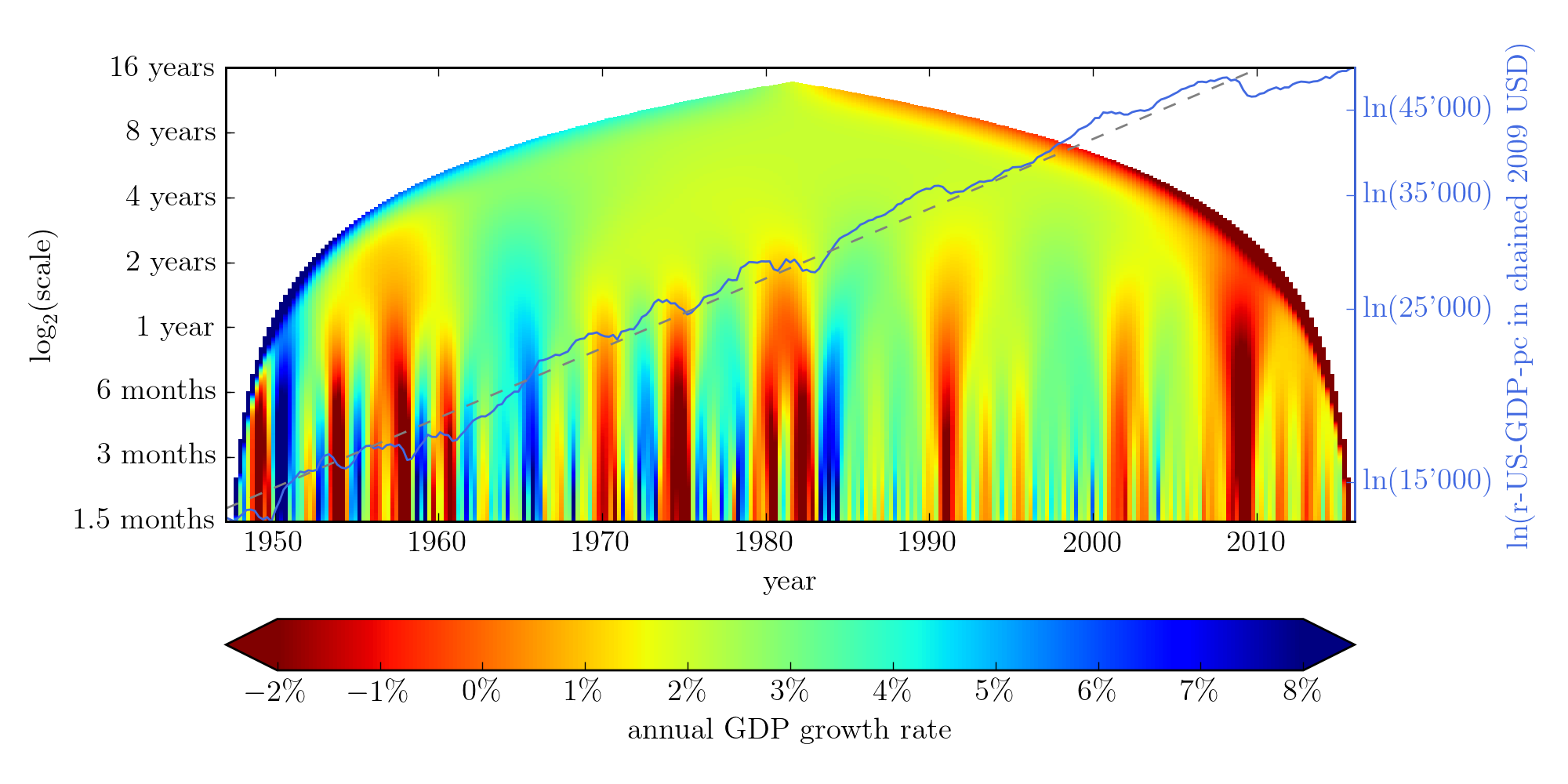
Figure 1: Wavelet transform $\ln(\text{r-US-GDP-pc})\ast\psi^{(1)}$ of the logarithm of the quarterly real US GDP per capita data measured in chained 2009 US dollar over the period from 1947 to 2015 and represented by the continuous dark line (right vertical axis). An ordinary least squares fit determines a long-term annualized growth rate $\rho_{\text{lt}}$ of approximately $2\%$, shown as the dashed line. The left vertical axis plots the scale $s$ of the wavelet analysis, corresponding to an interval of analysis approximately equal to $2s$. The color scale encodes the value of the annualized growth rates at different times and scales. The nonlinear conical shape of the envelop is due to edge-effects in the wavelet transform.

over the period from 1947 to 2015 shown on the horizontal axis. The left vertical axis plots the scale $s$ of the wavelet analysis, corresponding to an interval of analysis approximately equal to $2s$. For scales at and lower than $s\approx 4$ years (i.e. averaged over approximately 8 years), one can first observe a hierarchy of branches associated with alternating warm (low or negative growth rates) and cold (positive and strong growth rates) colors. As one goes to smaller and smaller time scales, more fine structures of alternating colors (growth rates) can be seen. At the larger scales, $s\geqslant 4$ years, the color settles to the green value, recovering the known, and also directly determined by OLS, long term growth $\rho_{\text{lt}}\approx 2\%$.

Because the continuous wavelet transform (1) with (2) contains a lot of redundant information (a function $X(t)$ of one variable $t$ is transformed into a function $W_{\psi}[X](s,t)$ of two variables $t$ and $s$), it is standard to compress the wavelet map shown in figure 1 into a so-called “skeleton” [35, 36, 37]. The skeleton of $W_{\psi}[X](s,t)$ is the set of all local maxima of $\left|W_{\psi}[X](s,t)\right|$ considered as a function of $t$, for fixed scale $s$. It is thus the set of all local maxima and minima of $W_{\psi}[X](s,t)$. The skeleton forms a set of connected curves in the time-scale space, called the extrema lines. Geometrically, each such skeleton line corresponds to either a crest or valley bottom of the three-dimensional representation of the wavelet function $W_{\psi}[X](s,t)$. A crest can be viewed as the typical value of the growth rate of a locally surging r-US-GDP-pc. The bottom of a valley is similarly the typical value of the growth rate of a locally slowing down or contracting r-US-GDP-pc.

The skeleton of figure 1 is shown in figure 2.

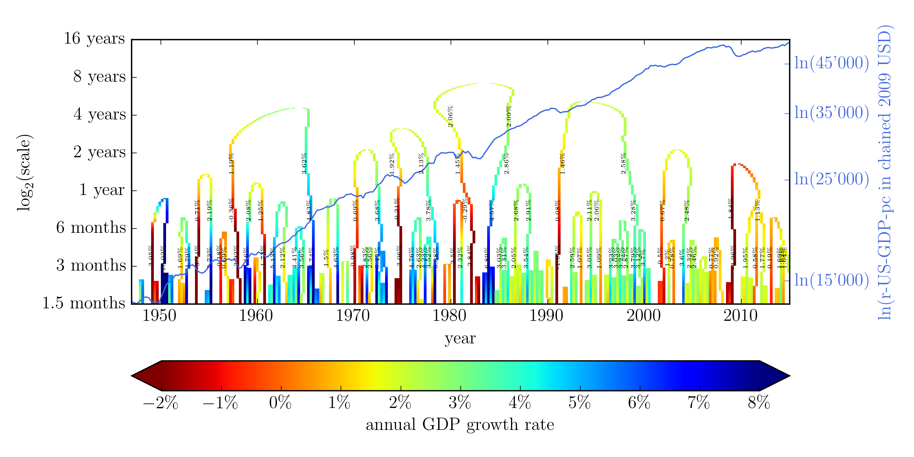
Figure 2: Skeleton structure of the wavelet transform $\ln(\text{r-GDP-pc})\ast\psi^{(1)}$ for quarterly real US GDP per capita data measured in chained 2009 US dollar corresponding to figure 1.

One can observe much more clearly the hierarchy of alternating growth regimes, which combine into an overall growth of $\approx 2\%$ at large scales. Written along each skeleton line in the figure, we give the values of the local annualized growth rates at four scale levels, 3 months, 6 months, 18 months and 3 years. The structure of the skeleton lines, their colors and the values of the local annualized growth rates confirm the existence of ubiquitous shifting regimes of slow and strong growths.

To validate the intuition that a crest (resp. valley bottom) of the skeleton can be viewed as the typical value of the growth rate of a locally surging (resp. slowing down) r-US-GDP-pc, we check that only knowing the growth rates on the skeleton structure retains the structural information of the full wavelet transform. For this, we have constructed synthetic versions of the real GDP per capita from the skeleton at different scales as explained in B, and we have compared them to the true r-US-GDP-pc.

3.3 Evidence for a robust bimodal structure of distributions of US GDP growth rates

The nature of the shifting regimes of slow and strong growths can be quantified further by constructing the probability density distributions (pdf) of annualized GDP growth rates at different fixed scales, both from the entire wavelet transform (figure 1) and from the skeleton structure (figure 2). The obtained pdf’s for four different scales (6, 9, 15 and 30 months) are depicted in figure 3.

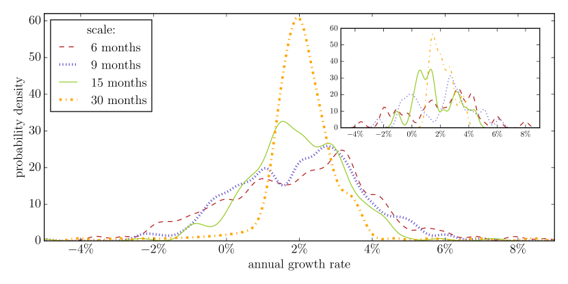
Figure 3: Gaussian kernel estimations (with width equal to $0.002$) of the probability density distributions (pdf) of the local annualized growth rates of r-US-GDP-pc at four different scales indicated in the inset in the top-left. The main panel represents the distributions extracted from the wavelet transform shown in figure 1, while the top-right inset shows the pdf’s obtained from the skeleton values shown in figure 2.

They have been obtained using a Gaussian kernel estimations with width equal to $0.002$. We have checked the robustness of these pdf’s by changing the width of the kernels within a factor of two.

The pdf’s extracted from the wavelet transform shown in figure 1 and from the skeleton values shown in figure 2 exhibit the same structures. First, the pdf’s at the largest scale of 30 months peak at the annualized growth rate of $\approx 2\%$, recovering the OLS value reported above (shown as the dashed line in figure 1). Second, as we go down to smaller scales, already at the scale of 15 months, and more pronounced at the scale of 9 and 6 months, a clear bimodal structure emerges (decorated by higher frequency structures, associated with the width of the estimating kernel). Denoting the two main peaks of the bimodal density extracted from the full wavelet transform (the skeleton gives similar results) at scale $s$ by $\rho_{\text{low}}(s)$ and $\rho_{\text{high}}(s)$ respectively, we obtain

$$\rho_{\text{low}}(6\text{ months})\approx 1\%\lesssim\rho_{\text{low}}(9\text{ months})\approx 1.1\%\lesssim\rho_{\text{low}}(15\text{ months})\approx 1.5\%\lesssim\rho_{\text{lt}}\approx 2\%$$ (4)

and

$$\rho_{\text{high}}(6\text{ months})\approx 3.1\%\gtrsim\rho_{\text{high}}(9\text{ months})\approx 2.8\%\approx\rho_{\text{high}}(15\text{ months})\approx 2.8\%\gtrsim\rho_{\text{lt}}\approx 2\%.$$ (5)

The pleasant stability for the estimates $\rho_{\text{low}}(6\text{ months})\approx\rho_{\text{low}}(9\text{ months})$ and $\rho_{\text{high}}(6\text{ months})\approx\rho_{\text{high}}(9\text{ months})\approx\rho_{\text{high}}(15\text{ months})$ suggests that real US GDP per capita can be modelled as an alternation of slow growth around a typical value of $1\%$ and strong growth around a typical value of $3\%$, which bracket the long-term average growth rate $\rho_{\text{lt}}\approx 2\%$. This constitutes the main result of our article.

A presents the wavelet transform, skeleton structure and growth rate distributions for annual r-US-GDP-pc data starting in 1800 till 2010. The important conclusion is that the previous observations presented above for quarterly data from 1950 to 2015 are broadly confirmed when using annual data over this much longer period.

4 Concluding remarks

We have presented a quantitative characterisation of the fluctuations of the annualized growth rate of the real US GDP per capita growth at many scales, using a wavelet transform analysis of two data sets, quarterly data from 1947 to 2015 and annual data from 1800 to 2010. Our main finding is that the distribution of GDP growth rates can be well approximated by a bimodal function associated to a series of switches between regimes of strong growth rate $\rho_{\text{high}}$ and regimes of low growth rate $\rho_{\text{low}}$. The succession of alternations of these two regimes compounds to produce a remarkably stable long term average real annualized growth rate of 1.6% from 1800 to 2010 and $\approx 2.0\%$ since 1950.

We thus infer that the robust constant growth rate since 1950 cannot be taken as evidence for a purely exogenous “natural” rate of innovations and productivity growth. It is rather a remarkable output of the succession of booms and corrections that punctuate the economic history of the US since more than 200 years. Our results suggest that alternating growth regimes are intrinsic to the dynamics of the US economy and appear at all scales. These alternating regimes can be identified as generalized business cycles, occurring at the scale of the whole economy.

Such business cycles may be briefly rationalised as follows. During the high growth regime, a number of positive feedback loops are in operation, such as deregulation, enhanced credit creation, the belief in a “new economy” and so on. This creates a transient boom, perhaps accelerating itself and leading to financial and social bubbles [38, 39, 40, 18, 19, 21]. This over heating of the economy then turns out not to be sustainable and leads to a correction and consolidation phase, the low growth regime. Then, the next strong growth regime starts and so on.

Our findings suggest that strong growth cannot be dissociated from periods of recessions, corrections or plateaus, which serve as a consolidation phase before the next boom starts. However, because of the remarkable recurrence of the strong regime and in view of its short-term beneficial effects, economists and policy makers tend to form expectations of strong continuous growth. Such way of thinking may lead to conclusions that, we argue, may have little merit. Consider the estimation of the US Federal Reserve Bank of Dallas [41] that the cost of the 2008 crisis, assuming output eventually returning to its pre-crisis trend path, is an output loss of $6 trillion to $14 trillion US dollars. These enormous numbers are based on the integration of the difference between the extrapolation of hypothetical GDP trajectories expected from a typical return to pre-crisis growth compared with the realised GDP per capita. In the light of our findings, we argue that it is incorrect to extrapolate to the pre-crisis growth rate, which is by construction abnormally high, and much higher than the long term growth rate. In addition, one should take into account the fact that the base rate after a crisis should be low or even negative, for the consolidation to work. Moreover, the duration of the boom years may have direct impact on that of the recovery period. In this vein, Sornette and Cauwels [17] have argued that this 2008 crisis is special, as it is the culmination of a 30 year trend of accelerating financialization, deregulation and debt growth. Our present results impel the careful thinker to ponder what is the “natural” growth rate and avoid naive extrapolations.

Using a simple generic agent-based model of growth, Louzoun et al. [16] have identified the existence of a trade off between either low and steady growth or large growth associated with high volatility. Translating this insight to the US economy and combining with the reported empirical evidence, the observed growth features shown in the present paper seem to reveal a remarkable stable relationship between growth and its fluctuations over many decades, if not centuries. Perhaps, this is anchored in the political institutions as well as in the psychology of policy makers and business leaders over the long term that transcend the short-term vagaries of political power sharing and geopolitics. It is however important to include in these considerations the fact that the US is unique compared with other developed countries, having benefitted enormously from the two world wars in particular (compared with the destruction of the UK and French empires and the demise of the economic dominance of european powers).

Appendix A Analysis of annual US GDP data

In this appendix, we present wavelet transform, skeleton structure and growth rate distributions for annual r-US-GDP-pc data starting in 1800 till 2010. The important conclusion is that the previous observations presented in the main text for quarterly data from 1950 to 2015 are broadly confirmed when using annual data over this much longer period.

Figure 4

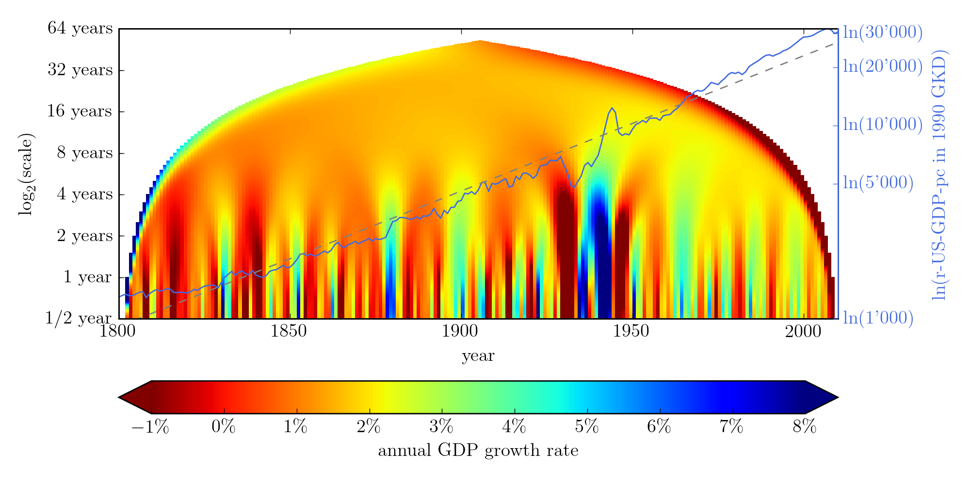
Figure 4: Wavelet transform $\ln(\text{r-US-GDP-pc})\ast\psi^{(1)}$ of the logarithm of the annual real US GDP per capita data measured in 1990 Geary-Khamis dollar and represented by the continuous dark line (right vertical axis). An ordinary least squares fit determines a long-term annualized growth rate $\rho_{\text{lt}}$ of approximately $1.6\%$.

shows the wavelet transform $\ln(\text{r-US-GDP-pc})\ast\psi^{(1)}$ of the logarithm of the annual real US GDP per capita data measured in 1990 Geary-Khamis dollar from 1800 to 2010 and represented by the continuous dark line (right vertical axis). An ordinary least squares fit determines a long-term annualized growth rate $\rho_{\text{lt}}$ of approximately $1.6\%$. This value is smaller than the average growth rate of $2\%$ determined for the period from 1950 to 2015. This smaller value is a compromise, given the rather clear long term upward curvature presented by the continuous curve shown in figure 4, expressing a tendency for the growth rate to grow itself [42]. Indeed, one can see that $ln(\text{r-US-GDP-pc})$ departs more and more from the dashed straight line with a larger slope after 1950, in line with the observations shown in figure 1. Figure 5 depicts the skeleton structure extracted from figure 4

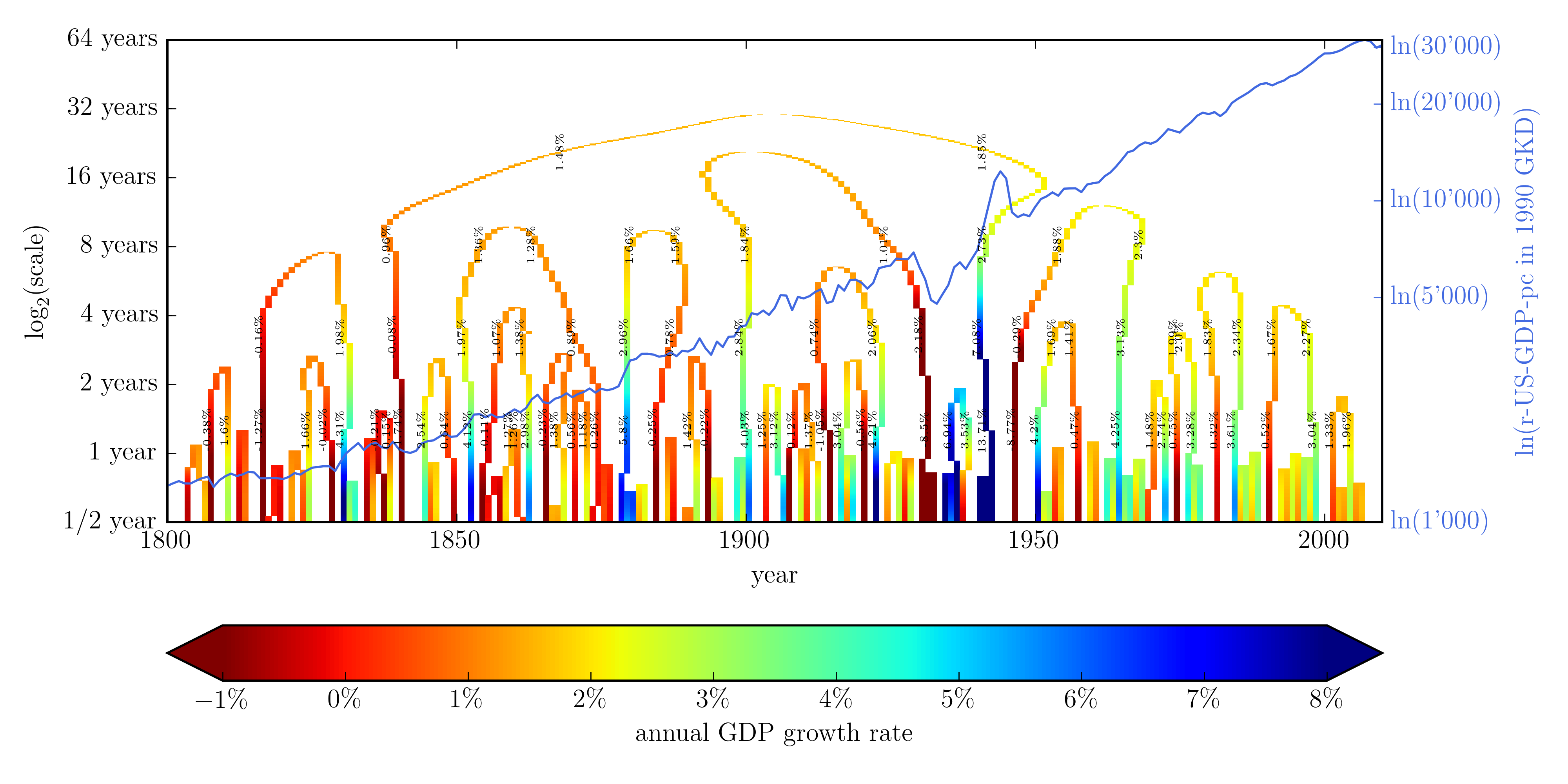
Figure 5: Skeleton structure of $\ln(\text{r-GDP-pc})\ast\psi^{(1)}$ for annual real US GDP per capita data measured in 1990 Geary-Khamis dollar corresponding to figure 4.

and figure 6

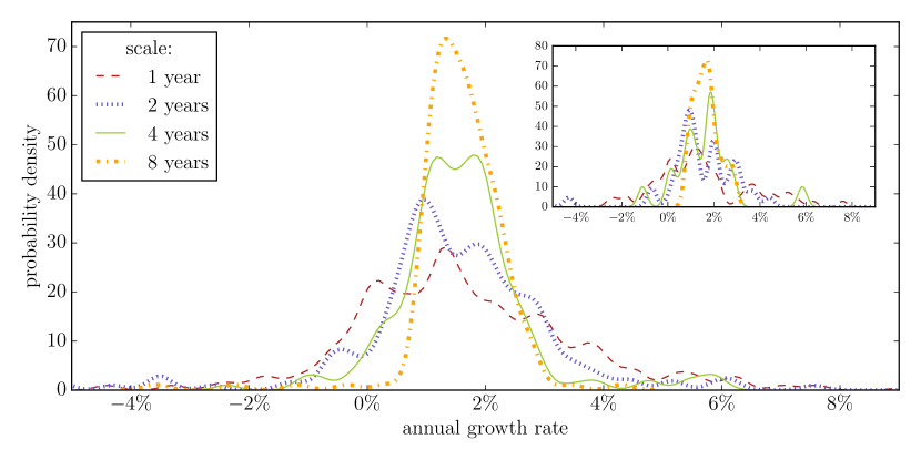
Figure 6: Gaussian kernel estimations (with width equal to $0.002$) of the probability density distributions (pdf) of the local annualized growth rates of r-US-GDP-pc sampled annually from 1800 to 2010 at four different scales indicated in the inset in the top-left. The main panel represents the distributions extracted from the wavelet transform shown in figure 4, while the top-right inset shows the pdf’s obtained from the skeleton values shown in figure 5.

plots the distribution of growth rates of the r-US-GDP-pc extracted from annual real US GDP per capita data since 1800. As for the quarterly GDP data, the long term growth rate of $\approx 1.5\%$ is recovered as the peak of the distribution at the $8$ year scale. The bimodal structure is less clean, due to the fact that annual sampling of GDP growth rates is bound to average over the time scales during which the transitions between the different regimes occur. Nevertheless, one can observe two main peaks, except for the largest time scale of $8$ years. Moreover, both at the $1$ and $2$ year scales, the estimated probability density functions (pdf) exhibit a positive skewness, with an asymmetric tail to the right side of large positive growth rates. This means that a considerable part of the probability mass is concentrated at high growth regimes above $\rho_{\text{lt}}$. Quantitatively, the values of the growth rates corresponding to the two main peaks of the pdf’s are: $\rho_{\text{low}}(1,2,4\text{ years})=0.2\%,1\%,1.2\%$ and $\rho_{\text{high}}(1,2,4\text{years})=1.4\%,1.9\%,1.8\%$. The rather low value $\rho_{\text{high}}(1\text{year})=1.4\%$ should be considered together with the evidence of the strong positive skewness noted above: at the annual sampling rate, the granularity of the data is too coarse to recover the clean picture of the quarterly data due to overlapping intervals. However, we find that the $50\%$-quantile growth rate is $1.3\%$, while the expectation value of the growth rates conditional on growth rates above $1.3\%$ is equal to $3.3\%$, much larger than $\rho_{\text{lt}}$. The results are thus in broad agreement with those presented in figure 3 for quarterly data.

Appendix B Synthetic GDP from wavelet skeletons

In figure 2 and figure 5, we have extracted the skeleton structure by keeping only local extrema as a function of time and discarding all additional information from the wavelet transform. In order to verify that the skeleton structure retains the most crucial information of the full wavelet transform, we construct here what we call the synthetic GDP, as follows:

1. Think of the skeleton structure of the real US GDP per capita (r-US-GDP-pc) growth rates shown in figure 5.

2. Fix a scale $s^{*}$.

3. Imagine a horizontal line at that fixed scale $s^{*}$. This line intercepts some $n=n(s^{*})$ skeleton arms of the wavelet transform. Denote the wavelet coefficient at the intercept of the horizontal line with the $i$-th arm by $g_{i}$. This results in a set of $n$ growth rates $g_{1},\ldots,g_{n}$.

4. Denote the time coordinate of the $g_{i}$ intercept by $t_{i}$. This way, we can uniquely label each $g_{i}$ as $g_{i}=g_{i}(t_{i};s^{*})$.

5. Denote the temporal separation between $g_{i-1}$ and $g_{i}$ by $\Delta t_{i}\equiv t_{i}-t_{i-1}$ (in units of years).

6. Denote the origin of time by $t_{0}$. In our annual r-US-GDP-pc data set, $t_{0}=1800$.

7. Define $\ln(\text{GDP}_{0})\equiv\ln\left(\text{r-US-GDP-pc in 1800}\right)$.

8. Then, the synthetic GDP at scale $s^{*}$ at time $t_{k}$ is calculated as

   $$\text{GDP}_{\text{pseudo}}(t_{k};s^{*})\equiv\text{GDP}_{0}\cdot\prod_{i=1}^{k}(1+g_{i})^{\Delta t_{i}}.$$ (6)

9. We expect $\text{GDP}_{\text{pseudo}}(t_{k})~{}\approx~{}$r-US-GDP-pc at time $t_{k}$ and to be approximately independent of the scale $s^{*}$.

We have calculated the synthetic GDP given by formula (6) at four different scales $s^{*}=1$ year, $2$ years, $4$ years and $8$ years. The result is depicted in figure 7. We see that the skeleton structure reproduces the real GDP quite accurately, thus confirming that the skeleton structure retains the most crucial features of the full wavelet structure. Notable deviations are observable around the sequence of peaks around the 1950s, where the discreteness of the skeleton structure leads to an overshooting or undershooting in the very unstable time associated with WWII and its aftermath, when the US GDP shot up to extraordinary level corresponding to the an outstanding war effort, following by a crash back to the long term trend. The distorsion to the long-term synthetic GDP brought by this period does not impact our study of the local growth rates and their bimodal distribution, being local in nature.

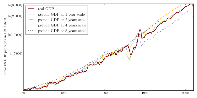
Figure 7: Synthetic real GDP per capita constructed using expression (6) at four different scales and comparison with the realized real US GDP per capita.

References

- [1] N.G. Mankiw. Principles of Economics, 5th edition. South-western Cengage Learning, 2011.
- [2] G. Erber. What is Unorthodox Monetary Policy? SSRN Working Paper, 2012.
- [3] E. Dabla-Norris, S. Guo, V. Haksar, M. Kim, K. Kochhar, K. Wiseman, and A. Zdzienicka. The new normal: a sector-level perspective on productivity trends in advanced economies. IMF staff discussion note SDN/15/03, 2015.
- [4] T. Holden. Medium-frequency cycles and the remarkable near trend-stationarity of output. Discussion Papers in Economics, Department of Economics, University of Surrey, DP 14/12, 2012.
- [5] J. G. Fernald and C. I. Jones. The Future of US Economic Growth. American Economic Review: Papers & Proceedings, 104(5):44–49, 2014.
- [6] R. J. Gordon. Is U.S. Economic Growth Over? Faltering Innovation Confronts the Six Headwinds. NBER Working Paper No. w18315., 2012.
- [7] G. D. Hansen. Indivisible labor and the business cycle. Journal of monetary Economics, 16(3):309–327, 1985.
- [8] M. Merz. Search in the labor market and the real business cycle. Journal of Monetary Economics, 36(2):269–300, 1995.
- [9] B.S. Bernanke, M. Gertler, and S. Gilchrist. The financial accelerator in a quantitative business cycle framework. volume 1, Part C of Handbook of Macroeconomics, pages 1341 – 1393. 1999.
- [10] L. Barseghyan, M. Battaglini, and S. Coate. Fiscal policy over the real business cycle: A positive theory. Journal of Economic Theory, 148(6):2223–2265, 2013.
- [11] R. D. Mclean and M. Zhao. The business cycle, investor sentiment, and costly external finance. Journal of Finance, 69(3):1377–1409, 2014.
- [12] D. Altig, L. J Christiano, M. Eichenbaum, and J. Linde. Firm-specific capital, nominal rigidities and the business cycle. Review of Economic Dynamics, 14(2):225–247, 2011.
- [13] B. Michele, J. C. Lawrence, and D. M. F. Jonas. Habit Persistence, Asset Returns, and the Business Cycle. The American Economic Review, 91(1):149–166, 2001.
- [14] Y. Kim and C. R. Nelson. Pricing Stock Market Volatility: Does it Matter whether the Volatility is Related to the Business Cycle? Journal of Financial Econometrics, 12(2):307–328, 2013.
- [15] R. Dalio. How the economic machine works. Bridgewater Associates, 2015.
- [16] Y. Louzoun, S. G. Solomon, J. Goldenberg, and D. Mazursky. World-size global markets lead to economic instability. Artificial life, 9(4):357–370, 2003.
- [17] D. Sornette and P. Cauwels. 1980-2008: The Illusion of the Perpetual Money Machine and what it bodes for the future. Risks, 2:103–131, 2014.
- [18] D. Sornette. Nurturing breakthroughs: lessons from complexity theory. Journal of Economic Interaction and Coordination, 3(2):165–181, 2008.
- [19] M. Gisler and D. Sornette. Exuberant innovations: the Apollo program. Society, 46(1):55–68, 2009.
- [20] M. Gisler and D. Sornette. Bubbles Everywhere in Human Affairs. Swiss Finance Institute Research Paper, (10–16), 2010.
- [21] M. Gisler, D. Sornette, and R. Woodard. Innovation as a social bubble: The example of the Human Genome Project. Research Policy, 40(10):1412–1425, 2011.
- [22] J. Morlet, G. Arens, E. Fourgeau, and D. Glard. Wave propagation and sampling theory-Part I: Complex signal and scattering in multilayered media. Geophysics, 47(2):203–221, 1982.
- [23] P. Goupillaud, A. Grossmann, and J. Morlet. Cycle-octave and related transforms in seismic signal analysis. Geoexploration, 23(1):85–102, 1984.
- [24] M. Antonini, M. Barlaud, P. Mathieu, and I. Daubechies. Image coding using wavelet transform. Image Processing, IEEE Transactions on, 1(2):205–220, 1992.
- [25] E. Slezak, A. Bijaoui, and G. Mars. Identification of structures from galaxy counts-Use of the wavelet transform. Astronomy and Astrophysics, 227:301–316, 1990.
- [26] F. Argoul, A. Arneodo, G. Grasseau, and Y. Gagne. Wavelet analysis of turbulence reveals the multifractal nature. Nature, 338:2, 1989.
- [27] Y. Meyer. Wavelets and applications. Springer-Verlag, 1992.
- [28] A. Grossmann and J. Morlet. Decomposition of Hardy functions into square integrable wavelets of constant shape. SIAM journal on mathematical analysis, 15(4):723–736, 1984.
- [29] P. Yiou, D. Sornette, and M. Ghil. Data-adaptive wavelets and multi-scale singular-spectrum analysis. Physica D, 142(3-4):254–290, 2000.
- [30] I. Daubechies. The wavelet transform, time-frequency localization and signal analysis. Information Theory, IEEE Transactions on, 36(5):961–1005, 1990.
- [31] I. Daubechies. Ten lectures on wavelets. SIAM, 1992.
- [32] L. Debnath and F. A. Shah. Wavelet transforms and their applications. Springer, 2002.
- [33] A. Arneodo, F. Argoul, J.F. Muzy, M. Tabard, and E. Bacry. Beyond classical multifractal analysis using wavelets: Uncovering a multiplicative process hidden in the geometrical complexity of diffusion limited aggregates. Fractals, 1(03):629—-649, 1993.
- [34] J. Miao and D. Xie. Economic growth under money illusion. Journal of Economic Dynamics & Control, 37(1):84–103, 2013.
- [35] A. Arneodo, B. Audit, N. Decoster, J.F. Muzy, and C. Vaillant. Wavelet Based Multifractal Formalism: Applications to DNA Sequences, Satellite Images of the Cloud Structure, and Stock Market Data. In The science of disasters, volume 2, page 27. Springer, 2002.
- [36] S. Mallat and S. Zhong. Characterization of signals from multiscale edges. IEEE Transactions on Pattern Analysis & Machine Intelligence, (7):710–732, 1992.
- [37] S. Mallat and W. L. Hwang. Singularity detection and processing with wavelets. Information Theory, IEEE Transactions on, 38(2):617–643, 1992.
- [38] P. Geraskin and D. Fantazzini. Everything you always wanted to know about log-periodic power laws for bubble modeling but were afraid to ask. The European Journal of Finance, 19(5):366–391, 2013.
- [39] D. Sornette and P. Cauwels. Financial bubbles: mechanisms and diagnostics. Review of Behavioral Economics, 2(3):279–305, 2015.
- [40] V.I. Yukalov, E.P. Yukalova, and D. Sornette. Dynamical system theory of periodically collapsing bubbles. The European Physical Journal B, 88(7):1–14, 2015.
- [41] T. Atkinson, D. Luttrell, and H. Rosenblum. How Bad Was It? The Costs and Consequences of the 2007-09 Financial Crisis. Staff Papers Federal Reserve Bank of Dallas, 20:1–22, 2013.
- [42] A. Johansen and D. Sornette. Finite-time singularity in the dynamics of the world population and economic indices. Physica A, 294(3-4):465–502, 2001.