Shortcut to adiabaticity in spinor condensates

Abstract

We devise a method to shortcut the adiabatic evolution of a spin-1 Bose gas with an external magnetic field as the control parameter. An initial many-body state with almost all bosons populating the Zeeman sublevel $m=0$, is evolved to a final state very close to a macroscopic spin-singlet condensate, a fragmented state with three macroscopically occupied Zeeman states. The shortcut protocol, obtained by an approximate mapping to a harmonic oscillator Hamiltonian, is compared to linear and exponential variations of the control parameter. We find a dramatic speedup of the dynamics when using the shortcut protocol.

I Introduction

Ultracold spinor Bose gases provide a beautiful example to study fragmented Bose-Einstein condensates (BEC) Mue , where Bose-Einstein condensation occurs in two or more single particle states simultaneously. This is an unusual scenario, in contrast with conventional Bose-Einstein condensation where bosons cluster together into a single state. For single-component bosons, condensation in a single state is enforced by repulsive interactions: The energetic cost of fragmentation is too high because of the associated exchange energy noz1995 .

For bosons with an internal degree of freedom, one can escape this mechanism by building correlations between the particles to cancel the exchange energy Mue . A spin-1 BEC with antiferromagnetic interactions in a tight trap has been predicted to host such fragmented condensates for vanishing magnetic fields law1998a ; ho2000a ; koashi2000a ; castin2001a ; zhou2003a ; barnett2010a ; Ger1 ; Ger2 . The atoms condense into a single spatial mode but there remains a large internal degeneracy at the single-particle level. Antiferromagnetic interactions lift this degeneracy, and lead to a total spin-singlet ground state which is completely fragmented between the three sublevels. The many-body singlet state displays strong quantum correlations, and has attracted much theoretical interest.

This spin-singlet fragmented condensate is fragile against any perturbation lifting the single-particle degeneracy, such as external magnetic fields ho2000a ; koashi2000a ; castin2001a . In experiments with alkali atoms, the most relevant perturbation is the quadratic Zeeman splitting between the Zeeman sublevels $m=0$ and $m=\pm 1$ stamperkurn2013a . For finite atom number $N$, there is a small but non-vanishing window where the singlet state survives as the quadratic Zeeman splitting increases from zero, before a crossover to a single $m=0$ condensate takes place (“single BEC domain”) barnett2010a ; Ger1 ; Ger2 . An appropriate witness of the transition is the variance $\Delta N_{0}\equiv\sqrt{\langle N_{0}^{2}\rangle-\langle N_{0}\rangle^{2}}$ which goes from $\propto N$ in the spin-singlet state to $\propto\sqrt{N}$ in an uncorrelated many-body state Ger2 .

Because of the sensitivity to external perturbations, the singlet state has so far eluded experimental observation. The gap to the first excited states is low and scales as the inverse of the number of atoms law1998a . Evaporative cooling used to produce quantum gases is unable to reach such ultralow temperatures. Another procedure is to adiabatically produce the singlet state by first applying a magnetic field and condensing in the $m=0$ state, and then slowly remove the field to produce the desired singlet state — see the sketch in Fig. 1. In order to stay adiabatic, the dynamics must be very slow in view of the small energy scales involved, making the procedure vulnerable to heating or inelastic losses.

In this article we introduce a way to shortcut the adiabatic following and thus produce the desired final state in times much shorter than those needed in adiabatic processes. Such methods have been recently derived for a number of quantum mechanical systems — see for instance Ref. torr12 , and promise to provide important advances in actual implementations of quantum technologies, for instance trapped ions adc16 . Exact protocols have been derived for particular problems, e.g. the quantum harmonic oscillator muga . In other cases, approximate procedures, obtained by adapting exact ones, have been proven to be quite promising when applied to quantum many-body systems Bru1 ; Bru2 ; sc15 .

As will be shown, the approximate shortcut protocol will be obtained from a large $N$ limit of the quantum many-body system. This limit will allow us to map our original many-spin problem into an effective harmonic oscillator, for which an exact solution is available muga . Interestingly, very recently a similar harmonic description of a spinor BEC has allowed the authors in Ref. chap to prove parametric amplification of a spinor system. This work proves experimentally the appropriateness of the harmonic description.

The article is organized as follows. In Section II, we present the theoretical model to describe the spinor BEC and discuss the adiabatic preparation of the ground state. In Section III we obtain our protocol to shortcut the adiabatic evolution in the spinor system from a continuum approximation to the spin dynamics. In Section IV we apply our shortcut protocol to the BEC regime (dominated by the quadratic Zeeman energy). In Section V we consider a broader range of parameters, discussing the quality of our protocol to produce fragmented BEC starting from the BEC side. In Section VI we present results making use of current experimental setups chap . In Section VII, we briefly summarize our work and present the main conclusions.

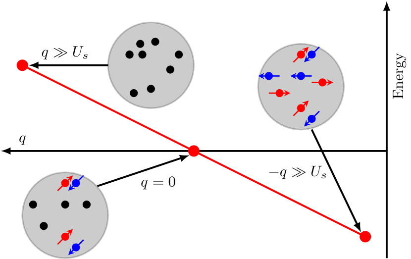
Figure 1: Sketch of the proposed experimental protocol. A spin-1 BEC is prepared at large positive values of the quadratic Zeeman energy (QZE) $q$ with all atoms in the $m=0$ state. In this regime, the initial state is very close to the ground state (arbitrarily close as $q\rightarrow\infty$). In the adiabatic method, the QZE is slowly reduced in such a way that the state of the system remains always close to the instantaneous ground state. Stopping the QZE ramp at $q=0$, the system ends up in a total spin-singlet ground state with strong spin correlations. Stopping the ramp at a large, negative value of $q$, we prepare instead a twin Fock state with half the atoms in the Zeeman $m=\pm 1$. In this paper we target the production of the singlet state, and examine this procedure and alternative ramps which are not adiabatic but result in a state close to the ground state in a much faster time.

II Theoretical Model

II.1 Description of the system

We consider an ultracold gas of spin-1 bosons in a harmonic trap under the action of an external magnetic field. We assume a single spatial mode in the trap, that is, all bosons condense in the same spatial orbit irrespective of their internal state. With this assumption we are left with three single-particle states, $|+1\rangle$, $|0\rangle$ and $|-1\rangle$, corresponding to the Zeeman states with magnetic quantum numbers $m=+1,0,-1$, respectively. The linear Zeeman effect acts only as a shift in the energy and does not contribute to determine the equilibrium state. The main contribution of the magnetic field is the quadratic, or second order, Zeeman (QZ) effect stamperkurn2013a . Under these assumptions, the system is well described by the Hamiltonian barnett2010a ; Ger1

$$\hat{H}=\frac{U_{s}}{2N}\ \hat{\bm{S}}^{2}-q\hat{N}_{0}\,,$$ (1)

where $U_{s}>0$ is the spin interaction energy per atom, $N$ is the number of atoms, ${\hat{\bm{S}}}^{2}$ is the (dimensionless) total spin operator, $q$ is the quadratic Zeeman energy and $\hat{N}_{m}$ is the number operator of the Zeeman state $m=0,\pm 1$.

The first term in the right-hand side of Eq. (1) describes antiferromagnetic interactions between pairs of atoms, and favours configurations with low total spin $S$. In absence of the quadratic Zeeman term, $q=0$, the eigenstates are known analytically and are given by the total spin eigenstates $|N,S,M\rangle$, where $S$ is the total spin and $M$ the eigenvalue of $\hat{S}_{z}$, the projection of the total spin on the $z$ axis. This is the basis we will be using in the following sections. Low-$S$ configurations are obtained by putting many spin-1 atoms to form singlet state pairs, while the remaining atoms can occupy any Zeeman sublevel. For practical convenience, from now on $N$ will be set to an even number. The ground state for even $N$ is the total spin singlet $|N,S=0,M=0\rangle$. This highly fragmented state, termed “spin-singlet condensate” (SSC), takes the form of a condensate of delocalized spin-singlet pairs,

$$|{\rm SSC}\rangle\propto \left(\hat{A}^{\dagger}\right)^{N/2}|\textrm{vac}\rangle$$ (2)

where $A^{\dagger}=(\hat{a}_{0}^{\dagger})^{2}-2\hat{a}_{+1}^{\dagger}\hat{a}_{-1}^{\dagger}$ creates a pair of atoms in the two-particle singlet state, $\hat{a}_{m}$ is an annihilation operator for a particle in the Zeeman state with third component of the angular momentum equal to $m$, and $|\textrm{vac}\rangle$ is the boson vacuum. This fragmented state is characterized by three macroscopically populated states, $\langle N_{+1}\rangle=\langle N_{0}\rangle=\langle N_{-1}\rangle=N/3$, with large fluctuations of the individual components Mue .

The second term in Eq. (1) describes the interaction of the system with the external magnetic field. In the non-interacting limit $U_{s}\rightarrow 0$ and for $q>0$, the QZE forces all the spins to occupy the state $m=0$, thus forming a single Bose-Einstein condensate with $\langle N_{0}\rangle=N$ and $\langle N_{+1}\rangle=\langle N_{-1}\rangle=0$, the so-called $z$-polar state,

$$|{\rm Polar}\rangle_{z}\propto\left(\hat{a}_{0}^{\dagger}\right)^{N}|\textrm{vac}\rangle\,.$$ (3)

It is worth noting that $M$ remains fixed when changing $q$, because the Hamiltonian commutes with $\hat{S}_{z}$. This is a good approximation to the behavior due to the experimental conditions of the atomic quantum gases, which are highly isolated from the environment, and to the microscopic rotational invariance of the spin exchange interaction stamperkurn2013a .

For simplicity, we take $M=0$. Also, as the number of particles $N$ is fixed during the evolution, we will omit it on the kets, thus, for now on we will use the notation $|S\rangle\equiv|N,S,0\rangle$.

II.2 Ground state for intermediate values of $|q|$

For generic values of $q,U_{s}$, we write a general state $|\phi\rangle$ with fixed $N$ and $M=0$ as $|\phi\rangle=\sum_{S}c_{S}|S\rangle$. The Schrödinger equation $\hat{H}|\phi\rangle=E|\phi\rangle$ in the $S$ basis reduces to the following discrete eigenvalue equation (see Appendix A),

$$h_{S,S+2}\,c_{S+2}+h_{S,S-2}\,c_{S-2}+h_{S,S}\,c_{S}=E\,c_{S}\,.$$ (4)

In the upper panel of Fig. 2 we show the transition from the $U_{s}$-dominated fragmented regime to the single BEC regime when varying the ratio $qN^{2}/U_{s}$. The transition between the two regimes takes place at values $qN^{2}U_{s}\simeq 1$ and is seen in the behavior of the variance $\Delta N_{0}/N$ of the populations in the $m=0$ Zeeman state. As explained in the introduction in the uncorrelated BEC state, $\Delta N_{0}\propto\sqrt{N}$, while in the spin-singlet state the fluctuations are much larger, $\Delta N_{0}\propto N$.

II.3 Adiabatic preparation of the singlet ground state

Experimentally, the value of the QZE can be controlled easily in real time. For instance, for Sodium atoms with hyperfine spin $F=1$ in a magnetic field $B$, the quadratic Zeeman shift contributes a positive amount to $q$. It is also possible to achieve $q<0$ by using the differential level shift induced on the individual Zeeman sublevels by a far off-resonant microwave field (see gerbier2006b for details). With a suitable choice of the microwave polarization, detuning and power, the sign and magnitude of $q$ can be changed at will.

This experimental control of the QZE opens a way to the generation of strongly correlated states in spin-1 quantum gases. The principle is the following. For zero magnetization and a large and positive QZE, the ground state is very close to a single BEC with all atoms in the $m=0$ Zeeman state. A good approximation of this state can be prepared “by hand”, e.g. by applying radio-frequency —rf— pulses with suitable frequency and polarization to a spin-polarized ensemble in $m=+1$, for instance. Starting from this initial state and decreasing slowly the value of $q$, the system will adiabatically follow its ground state, and end up prepared in the SSC state given in Eq. (2) when $q\approx 0$.

We can estimate the speed at which the magnetic field should be decreased by the usual adiabatic criterion, $|\langle j|\dot{H}|i\rangle|\ll\hbar\omega_{\rm ji}^{2}$, where $|i\rangle$ and $|j\rangle$ are two eigenstates of the Hamiltonian. The dangerous region is around $q<U_{s}/N^{2}$, where the energy gap to the first excited state takes its minimum value $\sim 3U_{s}/N$. In this region, the QZE ramp has to be very slow. We make a crude estimate by assuming that $q$ decreases between $U_{s}$ and $0$ in a time $\tau$. Also in this region, $N_{\pm 1}$ are on the order of $N/3$. This leads to $|\langle j|\dot{H}|i\rangle|\sim NU_{s}/3\tau$ and to the adiabaticity criterion,

$$\tau\gg\frac{N^{3}\hbar}{27U_{s}}.$$ (5)

The catastrophic scaling $\tau\propto N^{3}$ shows that this method will be limited to small, mesoscopic samples. Using very long ramp times to fulfill the adiabaticity criterion will make the protocol vulnerable to experimental limitations not captured by the single-mode Hamiltonian, such as technical heating (specific for each experimental setup) and inelastic losses (specific for each atom).

Inelastic atom losses destroy the rotational symmetry since atoms are lost at random from any Zeeman state. A common source of inelastic losses is three-body recombination into a weakly-bound molecule and a fast atom, resulting in three atoms lost from the trap. The total rate of these events can be written as $N\Gamma_{3}$, where $\Gamma_{3}=(K_{3B}/N)\int d^{3}\bm{r}\,n(\bm{r})^{3}$ is determined by a species-dependent rate constant $K_{3B}$ and by the spatial density $n$. Demanding less than one single inelastic event (on average) during the entire adiabatic protocol gives a bound $1/\tau\gtrsim N\Gamma_{3}$.

For illustrative purposes, we consider a gas of atoms condensing in the Gaussian ground state of a tight harmonic trap of frequency $\omega$. The Gaussian ground state of the trap is a good approximation of the actual condensate wavefunction for sufficiently low atom number $N<\sigma/\overline{a}$, with $\sigma=\sqrt{\hbar/m_{\rm A}\omega}$ the harmonic oscillator length, with $m_{\rm A}$ the atomic mass and with $\overline{a}$ the spin-independent $s-$wave scattering length. The spin-dependent scattering length $a_{s}$ is determined by the relation $U_{s}=(4\pi\hbar^{2}a_{s}/m_{\rm A}N)\int d^{3}\bm{r}\,n(\bm{r})^{2}$ law1998a . The bound $1/\tau\gtrsim N\Gamma_{3}$ can be written as a bound on the maximum affordable atom number in trap, written in compact form as

$$N\ll 5.1\left(\frac{\sigma}{l_{3B}}\right)^{3/5},$$ (6)

where $l_{3B}=(m_{\rm A}K_{3B}/\hbar a_{s})^{1/3}$ has the dimension of a length.

We specialize to the case of $F=1$ Sodium atoms, where $\overline{a}\approx 2.5\,$nm and $a_{s}\approx 0.1\,$nm knoop2011a and three-body loss rate constant $K_{3B}\sim 1.6\times 10^{-30}$at.cm⁶/s goerlitz2003a . Using $\omega/(2\pi)=2\,$kHz, one finds $N\ll 36$ for the parameters given above, showing that the adiabatic approach is reserved for mesoscopic samples containing only a few atoms. This motivates us to find alternative solutions enabling a substantial speed-up of the dynamics, which is our main objective in the rest of this paper.

III Shortcuts to adiabaticity

In view of the limitations of the adiabatic approach described above, we now examine a different method where the same final result can be reached in a much shorter time. In the literature, there are well-established shortcut protocols for one-body harmonic potentials muga . Our strategy is to use these results to manipulate the many-spin system of interest by mapping it to an effective harmonic oscillator problem. We show in this section how a reasonable harmonic approximation to the many-body problem can be derived. By means of such approximate equation we map the shortcut protocol to the exact time dependent Schrödinger equation built from Eq. (4).

III.1 Continuum approximation

The first step consists in deriving a continuum approximation to the Hamiltonian, Eq. (4). For large $N$ and considering $1\ll S\ll N$, the coefficients $c_{S}$ can be assumed to vary smoothly from $S$ to $S\pm 2$. Hence, $c_{S}$ can be approximated by a continuous function $c(x)$, where $x\equiv S/N$ varies from $0$ to $1$. Following the derivations in Appendix B, we arrive at an effective Schrödinger-like equation for a harmonic oscillator

$$-\frac{\hbar^{2}}{2M^{\ast}}c^{\prime\prime}(x)+\frac{M^{\ast}\omega^{2}}{2}x^{2}c(x)=(E+Nq)c(x)\,$$ (7)

with the oscillator frequency given by $\hbar\omega=\sqrt{q(q+2U_{s})}$ and the oscillator “mass” by $M^{\ast}/\hbar^{2}=N/2q$. The ground state obeying the boundary condition $c(0)=0$ is the wave function

$$c(x)= \frac{2\sqrt{2}}{(\pi\sigma)^{1/4}}\frac{x}{\sigma}\exp{\left(-\frac{x^{2}}{2\sigma^{2}}\right)}$$ (8)

$$\sigma= \sqrt{\frac{2}{N}}\left(\frac{q}{q+2U_{s}}\right)^{1/4}\,,$$ (9)

with energy

$$E=\frac{3}{2}\sqrt{q(q+2U_{s})}-Nq\,.$$ (10)

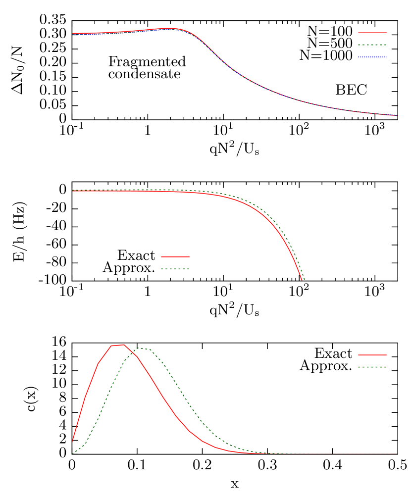
Figure 2: Upper panel: Fluctuation of the number of particles in the $m=0$ manifold, $\Delta N_{0}/N$ computed for three different number of atoms. Middle panel: Energy of the ground state of the exact system compared with the energy of the ground state obtained in Eq. (10) for different values of the parameter $q$. When $qN^{2}U_{s}^{-1}<2$, the system becomes $U_{s}$-dominated and, thus, the energy is constant [see Eq. (10)]. It is worth noting that both in the fragmented ($U_{s}$-dominated) and BEC ($q$-dominated) regimes, the approximate value of the energy agrees well with the exact one. Lower panel: Wave function of the ground state compared to the one obtained with the continuous approximation described in the text. The middle and lower panels are obtained for a system of $N=100$ spins. In all cases, $U_{s}/h=104.13$ Hz. For the lower panel, we have used $q=U_{s}$.

In Fig. 2 we compare the approximated and the exact solutions of our Hamiltonian. In the middle panel of Fig. 2 we see that the energy of the ground state is well reproduced by the harmonic approximation. In particular it is interesting to note that the harmonic approximation works well both in the $U_{s}$-dominated regime and in the $q$-dominated one. Comparing the actual wave functions in the lower panel of Fig. 2, we can see that the solution of the approximate Hamiltonian has a similar shape as the exact wave function although its maximum is slightly displaced towards higher values of $S/N$.

III.2 Shortcut protocol to the adiabatic evolution

The idea behind the shortcut to adiabaticity in the time-dependent evolution of an harmonic oscillator is the following. First we consider that the system is initially in the ground state for a certain initial value $q(0)$ of the control parameter. Then, we impose that at a given time $t_{f}$ the system must be exactly in the ground state for a different value of the control parameter, $q(t_{f})=q_{f}$. The goal is, thus, to find a function $q(t)$ that does the job. If the final time is sufficiently large, then any smooth ramp of the control parameter should work, since the evolution would be adiabatic. For short ramp times, an arbitrary ramp function would in general result in the excitation of many modes besides the ground state at the final time. The goal is therefore to engineer the ramp function in such a way as to minimize the excitations at $t=t_{f}$ and beyond, i.e. one seeks to produce an almost stationary state once the ramp is completed.

The Schrödinger-like equation in Eq. (7) is already close to the one corresponding to a harmonic oscillator. The control parameter is the QZE, $q=q(t)$. The term on the right-hand side (a shift in the total energy) does not have any effect on the dynamics. We also limit ourselves to the regime $q\ll U_{s}$. The final Schrödinger-like equation Eq. (7) is that of a harmonic oscillator with time-dependent “mass” and frequency $\omega^{2}(t)=2q(t)U_{s}/\hbar^{2}$. A similar equation was considered in Ref. Bru2 to describe the dynamics of a two-mode Bose-Hubbard model. Following the same method, we look for a self-similar solution $c(x)=c_{0}(x/\rho)/\sqrt{n}e^{i{\Theta(\rho,\dot{\rho}})}$, with a scaling parameter $\rho$. Such a solution exists if the scaling parameter obeys the so-called Ermakov equation muga ,

$$\ddot{\rho}+\omega(t)^{2}\rho=\frac{\omega_{0}^{2}}{\rho^{3}}.$$ (11)

The constant $\omega_{0}$ is just an integration constant that we set to $\omega_{0}=\frac{1}{\hbar}\sqrt{2q_{0}U_{s}}$. This, together with the substitution $b=1/\rho$ gives

$$\frac{2\dot{b}^{2}}{b}-\ddot{b}+\frac{2q(t)U_{s}}{\hbar^{2}}b=\frac{2q_{0}U_{s}}{\hbar^{2}}b^{5}.$$ (12)

$b(t)$ is an arbitrary function that only has to satisfy the frictionless conditions

$$\displaystyle b_{i}\equiv \,b(t_{0})=1\,,$$

$$\displaystyle b_{f}\equiv \,b(t_{f})=\left(\frac{q_{f}}{q_{0}}\right)^{1/4}\,,$$

$$\dot{b}(t_{0})= \,\dot{b}(t_{f})=\ddot{b}(t_{0})=\ddot{b}(t_{f})=0\,,$$

where $t_{0}$ will always be zero. There is an infinite set of functions $b(t)$ that can be used for this purpose, as the boundary conditions provide ample freedom to choose $b(t)$. Here we will use a simple polynomial ansatz, taken from Ref. muga ,

$$b(t)=b_{i}+10(b_{f}-b_{i})s^{3}-15(b_{f}-b_{i})s^{4}+6(b_{f}-b_{i})s^{5}\,,$$ (13)

where $s=t/t_{f}$. Thus, the function $q(t)$ is

$$q(t)=\left(2q_{0}U_{s}b^{4}+\hbar^{2}\frac{\ddot{b}}{b}-2\hbar^{2}\frac{\dot{b}^{2}}{b^{2}}\right)\frac{1}{2U_{s}}.$$ (14)

The six frictionless conditions previously mentioned uniquely determine the fifth-order polynomial chosen. We have tested that using a sixth-order polynomial or power-law functions did not improve the results, hence Eq. (13) is used in the rest of this work. Let us remark that the freedom in choosing $b(t)$ can be used to design more constrained protocols depending on the specific needs, e.g. avoiding too large values of $q(t)$.

IV Shortcut to adiabaticity in the BEC regime

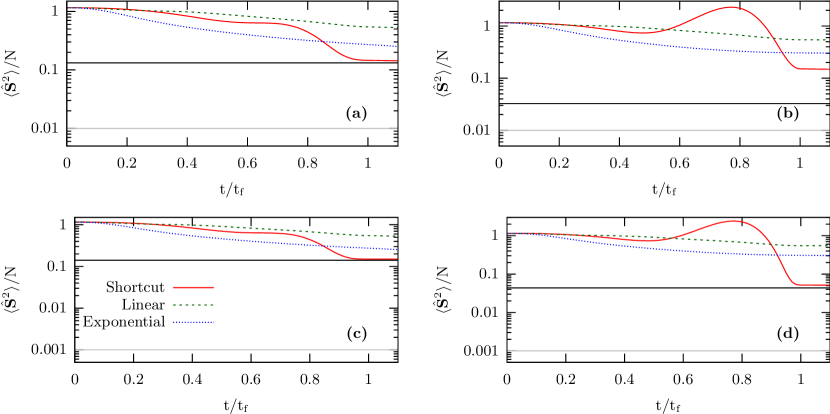
Figure 3: Mean squared spin $\langle\hat{\bm{S}}^{2}\rangle$ as a function of time computed for systems with $N=100$ and $N=1000$ spins evolved following either the shortcut protocol, a linear or an exponential ramps. All cases describe the evolution of the exact solution of the Schrödinger equation in situations where the evolution is clearly not adiabatic. Only the shortcut protocol brings the system to a state with lower total spin $S$. In all panels the initial state corresponds to $N^{2}q_{0}/U_{s}=N^{2}$, thus deep in the BEC phase (see Fig. 1 of Ger1 ). Panels on the left, —(a) and (c)— target a state at $N^{2}q_{f}/U_{s}=0.01N^{2}$, whereas right panels (b) and (d) correspond to a final state closer to the fragmented phase $N^{2}q_{f}/U_{s}=0.001N^{2}$. (a) and (b) correspond to $N=100$ while (c) and (d) are computed with $N=1000$. The horizontal solid black and light grey lines show the level of fluctuations in the ground state for $q=q_{f}$, and $\langle\hat{\bm{S}}^{2}\rangle=1/N$, respectively. In all cases, $U_{s}/h=104.13$ Hz and $t_{f}=0.01$ s.

In this Section, we consider the performance of our shortcut protocol in the BEC regime. That is, our main goal is to evolve from the ground state of Eq. (1) for an initial value of $q(t=0)=q_{0}=U_{s}$ to the corresponding ground state for $q(t_{f})=q_{f}$ such that $q_{0}>q_{f}\gg U_{s}/N^{2}$. Strictly speaking, the choice $q_{0}=U_{s}$ does not comply with the assumption used to derive the protocol, $q(t)\ll U_{s}$. The reason why the protocol can be extended to this situation is that for short times $t\lesssim t_{f}/4$, the protocol produces a very small variation of $q$, and the dynamics thus remains mostly adiabatic.

To judge the quality of the shortcut protocol we will compare it to two other ramps shapes, linear and exponential,

$$q_{\rm lin}(t)= q_{0}-(q_{0}-q_{f})\,t/t_{f}\,,$$ (15)

$$q_{\rm exp}(t)= (q_{0}-q_{f})\frac{e^{-\alpha t/t_{f}}-e^{-\alpha}}{1-e^{-\alpha}}+q_{f}\,.$$

The linear ramp is uniquely determined, and the exponential ramp was found to provide the best results for a decay constant $\alpha=5$, a value we have used in all the reported results.

We benchmark our shortcut protocol by numerically solving the full time dependent Schrödinger equation with $\hat{H}$ from Eq. (1) for a particular ramp. We used the mean-squared spin $\langle\hat{\bm{S}}^{2}\rangle$ as a fidelity witness. Note that in the regime we consider in this Section, the target final value of $q_{f}$ is far above the value $\sim U_{s}/N^{2}$ below which the ground state reduces to the total spin singlet state. As a result, the value of $\langle\hat{\bm{S}}^{2}\rangle$ in the ground state corresponding to $q_{f}$ fulfills $1\ll\langle\hat{\bm{S}}^{2}\rangle\ll N$.

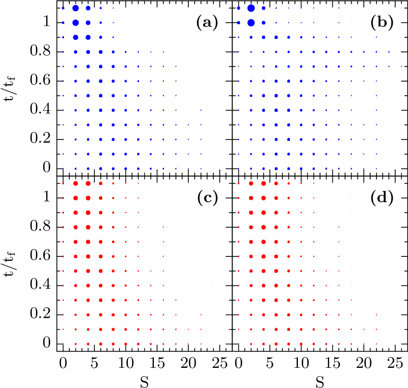
Figure 4: Time evolution of the wave function. The radii of circles indicate the value of $|c_{S}|^{2}$ for each $S$ at each time $t/t_{f}$. Blue circles correspond to a system evolved using the shortcut protocol and red circles correspond to a system evolved with an exponential ramp. Panels (a), (c) show the evolution of a system from $q_{0}/h=104.13$ Hz to $q_{f}=10^{-2}q_{0}$ in $t_{f}=0.01$ s and panels (b), (d) show the evolution of a system from $q_{0}/h=104.13$ Hz to $q_{f}=10^{-3}q_{0}$ in $t_{f}=0.01$ s, so this figure can be directly compared to Fig. 3. Since only the even solution is considered, the wave function $c_{S}$ at odd $S$ is identically 0.

In Fig. 3 we present the first results, corresponding to two different dynamical situations. The first one shown in Fig. 3 (a,c) goes from $q_{0}/U_{s}=1$ to $q_{f}/U_{s}=0.01$. The second one shown in Fig. 3 (b,d) goes one order of magnitude smaller, to $q_{f}/U_{s}=0.001$. Also we compare in the figure two different values of $N=100$ and $1000$. Several features can be observed. In all cases, the shortcut protocol performs clearly better than the other two ramps, while the exponential ramp performs better than the linear ramp. The spin witness $\langle\hat{\bm{S}}^{2}\rangle$ at the final time at $t_{f}=0.01\,$s is substantially lower for the shortcut protocol ($\langle\hat{\bm{S}}^{2}\rangle$ decreases by an order of magnitude from its initial value), and closer to the value expected in the final ground state for larger $N$. In comparison, the other two protocols are only able to decrease it by at most a factor of 4 in the same time. Moreover, the final value of $\langle\hat{\bm{S}}^{2}\rangle$ decreases with increasing atom number at a fixed $t_{f}$. Equivalently, the final fidelities obtained with the shortcut protocol improve as we increase $N$. This could be expected as we have obtained our protocol in the large $N$ limit, thus making the protocol closer to an exact description as $N$ is increased. The results obtained with the exponential and linear ramps are mostly independent of the number of particles.

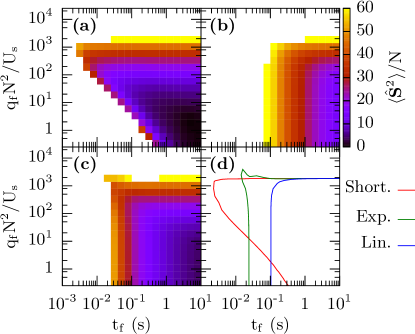
Figure 5: Value of $\langle\hat{\bm{S}}^{2}\rangle$ after the time evolution, i.e. $t=t_{f}$, for the three different protocols considered: shortcut (a), linear (b) and exponential (c). In all cases only the results that give $\langle\hat{\bm{S}}^{2}\rangle<60$ are shown. Finally, in (d), we show the contour lines corresponding to $\langle\hat{\bm{S}}^{2}\rangle=60$ . In all cases we have $N=500$ particles and an initial value of $q_{0}/h=0.1\,U_{s}/h=10.413$ Hz.

It is also interesting to see how the wave function evolves in time, going from a state with large $\langle\hat{\bm{S}}^{2}\rangle$, where $c_{S}$ are centered around large $S$, to a state with small $\langle\hat{\bm{S}}^{2}\rangle$, where the wave function takes substantial values around $S=0$ or $S=2$. In Fig. 4 we compare the wave functions at different times obtained with the shortcut (a,b) and exponential (c,d) protocols. The calculations correspond to the $N=100$ ones reported in Fig. 3. As can be clearly seen in all cases the wave function for the shortcut is much more peaked around $S=0$ than the exponential one. Also, as expected, the final wave function is more concentrated at smaller values of $S$ as we target final states with smaller $q_{f}$. This can be seen comparing panels (a,c), computed with $q_{f}N^{2}/U_{s}=0.01N^{2}$ with panels (b,d), computed with $q_{f}N^{2}/U_{s}=0.001N^{2}$. Finally, note that even though the shortcut performs quite well, the final wave function is peaked at $S=2$ rather than at $S=0$, which reflects the fact that we are still on the single BEC side of the crossover reported in Fig. 2 (c).

V Shortcut from BEC to a fragmented condensate

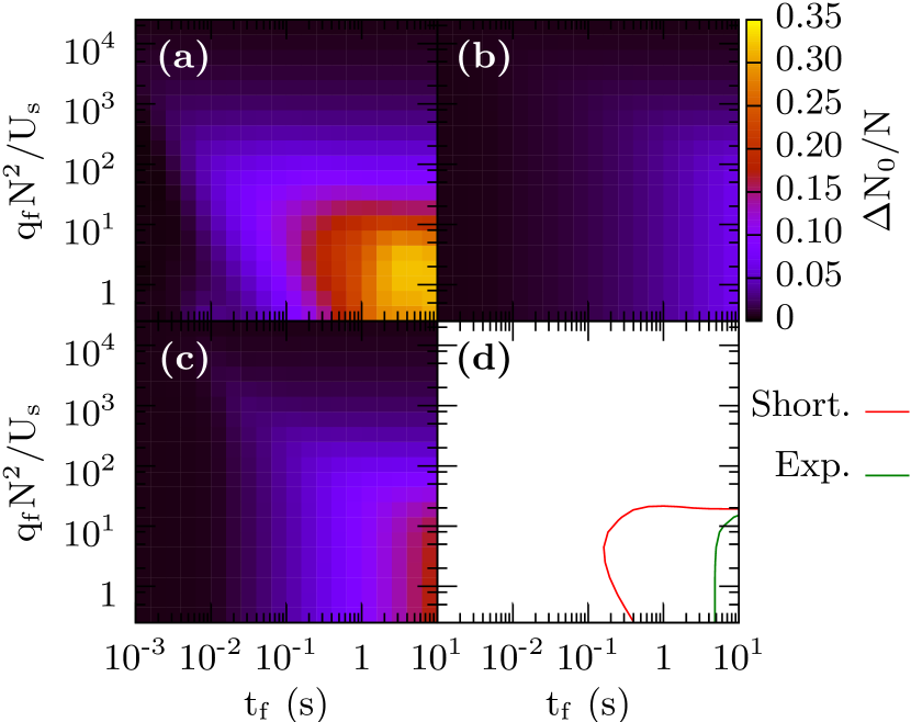
Figure 6: $\Delta N_{0}/N$ for the same conditions as in Fig. 5. The results obtained from the three different protocols, the shortcut, a linear ramp and an exponential one are given in panels (a), (b) and (c), respectively. Finally, in (d) we show the contour lines of the three cases above for $\Delta N_{0}/N=0.15$ . All these plots have been realized using a system of $N=500$ particles and $q_{0}/h=0.1\,U_{s}/h=10.413$ Hz.

In the previous section we have shown the superior performance of the shortcut protocol in comparison with exponential and linear ramps in the BEC regime, $qN^{2}/U_{s}\gg 1$. In this section we explore the fragmented condensate domain, that is, QZE ramps going from $q_{0}N^{2}/U_{s}\gg 1$ to $q_{f}N^{2}/U_{s}\lesssim 1$.

In Figs. 5 and 6, we provide an extensive comparison between our shortcut protocol and linear and exponential ramps. The figures depict the final values of $\langle\hat{\bm{S}}^{2}\rangle$, Fig. 5, and $\Delta N_{0}/N$, Fig. 6. In those figures we consider $N=500$ atoms, starting from the ground state corresponding to a value of $q_{0}=0.1U_{s}$. The figures cover a broad range of final target values of $q_{f}$ ranging from deep in the BEC sector into well below the transition to the fragmented condensate region, $q_{f}N^{2}/U_{s}\lesssim 1$, see Fig. 2 (Upper panel). Results are also reported as a function of the desired final time, $t_{f}$. We take again $U_{s}/h=104.13$ Hz and final times ranging from $0.001$ to $10$ seconds.

As found previously, the shortcut protocol performs better than the exponential and linear ramps in the BEC region, as can be seen looking at the $q_{f}N^{2}/U_{s}\gtrsim 1$ region in the three figures. For instance the region in the $(q_{f}N^{2}/U_{s},t_{f})$ map, where small final values of $\langle\hat{\bm{S}}^{2}\rangle$ are larger for the shortcut protocol. The exponential produces also relatively low values, with a result mostly independent of the value of $q_{f}$, while the linear ramp fails to produce small final values, unless $t_{f}\simeq 10$ s.

In situations in which the target final state is clearly in the fragmented domain, $q_{f}N^{2}/U_{s}\simeq 1$, the only method that produces sizeable fragmentation, as measured by $\Delta N_{0}/N\gtrsim 0.15$, is the shortcut protocol (see Fig. 6). The exponential ramp requires times almost two orders of magnitude larger to obtain the same level of fragmentation in the system. In line with the latter, lower final values for $\langle\hat{\bm{S}}^{2}\rangle$ are obtained for the shortcut protocol for those cases in which the fragmentation is closer to the singlet value $\Delta N_{0}/N\simeq\sqrt{4/45}=0.298$ Ger1 . For the parameters considered here, a shortcut ramp performed in $t_{f}\sim 1\,s$ is able to produce a state very close to the ground state, for $N=500$. Note that, using the notations and assumptions of Section II.3, the chosen value of $U_{s}/h\approx 10\,$Hz is achieved in a trap of frequency $\omega/(2\pi)\approx 300\,$Hz for $N=500$. The corresponding three-body lifetime is $\Gamma_{3}\approx 1300\,$s^-1, or $N\Gamma_{3}t_{f}\approx 0.4$: Less than a single three-body loss event (on average) during the entire shortcut protocol. Losses should not be a concern for $N\sim 500$.

VI Comparison with current experimental setups

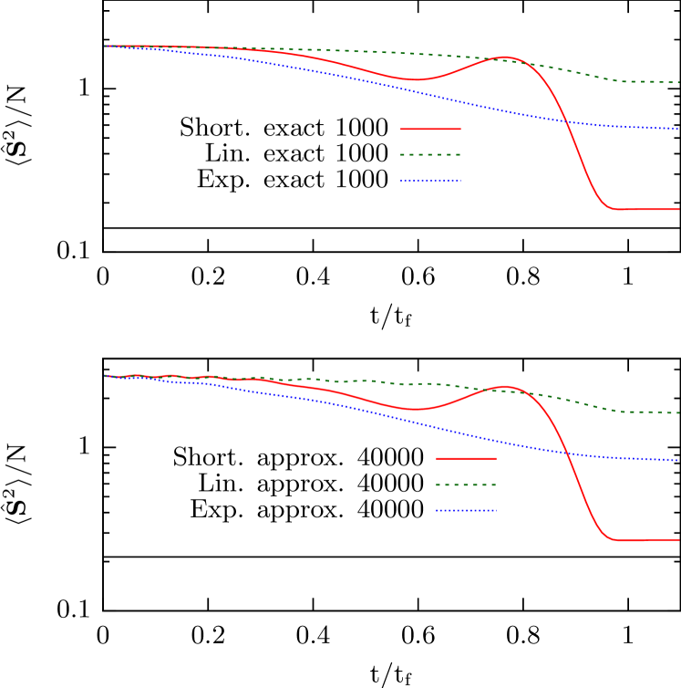
Figure 7: $\langle\hat{\bm{S}}^{2}\rangle$ as a function of time computed for systems evolved following the shortcut protocol, a linear or an exponential ramp. We compare together a system of $N=1000$ spins (exact solution) and a system with $N=40000$ spins (approximate solution). The system is evolved from a state with $q_{0}/h=10\,U_{s}/h=71$ Hz to $q_{f}=10^{-3}q_{0}$ in $t_{f}=0.1$ s. The shortcut protocol also works for this set of parameters, although it is, in principle, only valid for $q(t)\ll U_{s}$, in the sense that it provides a clear gain over simpler exponential or linear ramps.

We have been using, throughout the full manuscript, parameters taken from realistic proposals, most of them from Ger1 . In this Section, we explore different parameters taken from other experimental setups. Some experiments chap have been recently done with ⁸⁷Rb Bose condensates composed of $N=40000$ atoms with $U_{s}/h=7.1$ Hz and a $q(t)$ around $10\,U_{s}$. Taking these parameters, we have calculated the evolution of a system with $N=1000$ particles and $U_{s}/h=7.1$ Hz to check whether the shortcut protocol still gives good results under these experimental conditions. Results have also been obtained for a system with $N=40000$ spins using the shortcut protocol for the approximate Hamiltonian in Eq. (7). In Fig. 7 both results are shown for comparison.

$\langle\hat{\bm{S}}^{2}\rangle$, shown in Fig. 7, has been computed for these two systems and, although the initial values of $q(t)$ are larger than $U_{s}$, the shortcut protocol still drives the system to the ground state (or close) and improves the performance of the other two ramps. Although the shortcut protocol is, in principle, only valid for $q(t)\ll U_{s}$, this and other calculations (where we have driven a system from different values of $q_{0}$, all between 10 and 1000 times larger that $U_{s}$, to $q_{f}$ above and below $U_{s}$) show that the protocol can be successfully applied for larger $q_{0}$ values.

VII Summary and conclusions

We have presented a method to prepare a spin-1 BEC into a many-body spin singlet state by making use of an approximate protocol to shortcut the adiabatic following in the many-body system. The protocol consists in specific functions $q(t)$ which are constructed such that the time evolution of the system brings the many-body state from the ground state for $q_{0}\equiv q(t=0)$ to the ground state for $q_{f}\equiv q(t=t_{f})$. The main aim is to produce the very fragmented ground state of the spinor system in absence of quadratic magnetic field, starting from a condensate in the $m=0$ manifold in a regime dominated by the quadratic Zeeman term. The performance of the shortcut protocol has been compared to both a linear and an exponential ramp of the parameter $q$.

Even though the protocol is only approximate, it is shown to provide a much better performance than the exponential and linear ones almost in all situations. In the BEC side, that is, for $qN^{2}/U_{s}\gg 1$, the method works almost perfectly for time intervals of the order of $1/U_{s}$ and larger. The method works also better for cases in which the BEC-Fragmented transition is targeted. In particular it works with similar accuracy as the exponential ramp up to times one order of magnitude smaller. To quantify the performance we have computed the achieved final value of $\langle\hat{\bm{S}}^{2}\rangle$ and the value of $\Delta N_{0}/N$.

We have obtained results for systems with different sizes and final and initial setups and we have seen that the protocol achieves better results for larger systems. Results have also been obtained from approximate solutions of the Schrödinger equation [using Eq. (7) and (8)]. Based on these results we have been able to extrapolate the method to larger systems and find that, with this protocol, a many-body spin singlet state can be obtained for many different systems sizes. We have also shown the success of our method when applied to systems prepared with parameters taken from current experimental setups. We believe that our method for preparing a BEC into a singlet state with short times is experimentally realizable and efficient. Further improvements to the shortcut protocol profiting from the available freedom inherent to the presented procedure will be the object of forthcoming investigations.

Appendix A Eigenstates of the Hamiltonian in the $|N,S,M\rangle$ basis

The Hamiltonian in Eq. (1) is diagonalized by the total spin eigenstates $|N,S,M\rangle$, where $S$ is the total spin and $M$ the total projection of $S$ in the z-axis direction. A general state $\phi_{M}$ is written as, $|\phi_{M}\rangle=\sum_{S=|M|}^{N}c_{S}|N,S,M\rangle$. The construction of the angular momentum eigenstates is not trivial and these are built as follows law1998a ; ho2000a ; koashi2000a ; castin2001a ; Ger1 ,

$$|N,S,M\rangle=\frac{1}{\mathcal{Z}(N,S,M)^{1/2}}\left(\hat{S}_{-}\right)^{P}\left(\hat{A}^{\dagger}\right)^{Q}\left(\hat{a}_{+1}^{\dagger}\right)^{S}|{\rm vac}\rangle\,,$$ (16)

where $P=S-M$, $2Q=N-S$, $\hat{a}_{i}^{\dagger}$ and $\hat{a}_{i}$ are the creation and annihilation operators of the state $i$ respectively, $\hat{S}_{-}=\sqrt{2}(\hat{a}_{-1}^{\dagger}\hat{a}_{0}+\hat{a}_{0}^{\dagger}\hat{a}_{+1})$ is the lowering total spin operator and $\hat{A}^{\dagger}=(\hat{a}_{0}^{\dagger})^{2}-2\hat{a}_{+1}^{\dagger}\hat{a}_{-1}^{\dagger}$ is the singlet creation operator.

The expression of these states involves three operators. The first one, $\hat{a}_{+1}^{\dagger}$ is the creation operator of a spin $1$ particle with $m=+1$. This operator acting $S$ times over the vacuum leads to the many-particle state $\propto|S,S,S\rangle$. The following acting operators $\hat{A}^{\dagger}$ and $\hat{S}_{-}$ commute with the total spin momentum operator and therefore do not modify $S$. The singlet creator operator creates pairs with total spin $0$, so it only changes the number of particles. Then, $Q$ repeated actions of this operator add singlet pairs until the state $\propto|N,S,S\rangle$ is obtained. Finally, the lowering angular momentum operator $S_{-}$ acts $P=S-M$ times without affecting $N$ or $S$, leading to the final state $\propto|N,S,M\rangle$. The normalization factor is obtained after tedious calculations,

$$\mathcal{Z}(N,S,M)=S!\ \frac{(N-S)!!(N+S+1)!!}{(2S+1)!!}\ \frac{(S-M)!(2S)!}{(S+M)!}\,.$$ (17)

The complete Hamiltonian in Eq. (1) can be computed in the $N,S,M$ basis. The interaction term is diagonal, but the operator $\hat{N}_{0}=\hat{a}_{0}^{\dagger}\hat{a}_{0}$ has matrix elements between states with $S$ and $S\pm 2$. The total Hamiltonian is thus tridiagonal and therefore easy to solve numerically. The action of $\hat{N}_{0}$ is explicitly given by Ger1 ,

$$q\hat{N}_{0}|N\ S\ M\rangle=$$ (18)

$$= q\sqrt{A_{-}(N,S+2,M)A_{+}(N,S,M)}|N\ S+2\ M\rangle+$$

$$+ q\sqrt{A_{+}(N,S-2,M)A_{-}(N,S,M)}|N\ S-2\ M\rangle+$$

$$+ q\left[A_{-}(N,S,M)+A_{+}(N,S,M)\right]|N\ S\ M\rangle\,,$$

where

$$A_{+}(N,S,M) = \frac{(S+M+1)(S-M+1)(N-S)}{(2S+1)(2S+3)}\,,$$

$$A_{-}(N,S,M) = \frac{(S+M)(S-M)(N+S+1)}{(2S+1)(2S-1)}\,.$$ (19)

The resulting Hamiltonian, given also in Eq. (4), reads,

$$h_{S,S+2}\,c_{S+2}+h_{S,S-2}\,c_{S-2}+h_{S,S}\,c_{S}=E\,c_{S}\,.$$ (20)

with

$$h_{S,S+2} = -q\sqrt{(N+S+3)(N-S)}$$

$$\times \frac{(S+1)(S+2)}{(2S+3)\sqrt{(2S+1)(2S+5)}},$$

$$h_{S,S-2} = -q\sqrt{(N+S+1)(N-S+2)}$$

$$\times \frac{S(S-1)}{(2S-1)\sqrt{(2S+1)(2S-3)}},$$

$$h_{S,S} = \frac{U_{s}}{2N}S(S+1)$$

$$- q\left[\frac{S^{2}(N+S+1)}{(2S-1)(2S+1)}+\frac{(S+1)^{2}(N-S)}{(2S+1)(2S+3)}\right]\,.$$

Appendix B Continuum approximation of the Hamiltonian

A continuum approximation of Eq. (4) can be obtained by considering $1\ll S\ll N$. The wave function $c_{S}$ can, thus, be approximated by a continuous function $c(x)$, where $x\equiv S/N$ and varies from $0$ to $1$. Then, $\epsilon=2/N$ can be taken as a small parameter and a Taylor expansion can be made,

$$c_{S\pm 2}=c(x)\pm\epsilon c^{\prime}(x)+\frac{\epsilon^{2}}{2}c^{\prime\prime}(x)+\mathcal{O}(\epsilon^{3})\,.$$ (22)

By substituting this expression into Eq. (4) the following continuum Schrödinger equation is obtained

$$\alpha(x)c^{\prime\prime}(x)+\beta(x)c^{\prime}(x)+\left(\gamma(x)-E\right)c(x)=0\,,$$ (23)

where

$$\alpha(x) = \frac{\epsilon^{2}}{2}(h_{S,S+2}+h_{S,S-2})\,,$$

$$\beta(x) = \epsilon(h_{S,S+2}-h_{S,S-2})\,,$$ (24)

$$\gamma(x) = h_{S,S}+h_{S,S+2}+h_{S,S-2}\,.$$

Taking into account that $1\ll S\ll N$, we can set the order until which we want to approximate. Performing a Taylor expansion in $S/N$, $1/S$ and $1/N$, and substituting the resulting expressions in Eqs. (24), one finds

$$\alpha(x) \approx -\frac{q}{N}\left(1-\frac{x^{2}}{2}+\frac{3}{2N}\right)\,,$$

$$\beta(x) \approx \frac{-q}{4N^{2}x^{2}}\left(1-\frac{x^{2}}{2}+\frac{3}{2N}\right)\,,$$ (25)

$$\gamma(x) \approx \frac{N}{2}U_{s}x^{2}-qN\left(1-\frac{x^{2}}{4}+\frac{1}{2N}+\frac{1}{8N^{2}x^{2}}\right)\,.$$

Keeping terms to leading order in $1/N,x$ we arrive at the Schrödinger-like equation (7).