Phase transitions in edge-weighted exponential
random graphs

Mei Yin Department of Mathematics, University of Denver, Denver, CO 80208, USA mei.yin@du.edu
Abstract.

The exponential family of random graphs represents an important and challenging class of network models. Despite their flexibility, conventionally used exponential random graphs have one shortcoming. They cannot directly model weighted networks as the underlying probability space consists of simple graphs only. Since many substantively important networks are weighted, this limitation is especially problematic. We extend the existing exponential framework by proposing a generic common distribution for the edge weights and rigorously analyze the associated phase transitions and critical phenomena. We then apply these general results to get concrete answers in exponential random graph models where the edge weights are uniformly distributed.

1. Introduction

Exponential random graphs are among the most widespread models for real-world networks as they are able to capture a broad variety of common network tendencies by representing a complex global structure through a set of tractable local features. These rather general models are exponential families of probability distributions over graphs, in which dependence between the random edges is defined through certain finite subgraphs, in imitation of the use of potential energy to provide dependence between particle states in a grand canonical ensemble of statistical physics. They are particularly useful when one wants to construct models that resemble observed networks as closely as possible, but without going into details of the specific process underlying network formation. For history and a review of developments, see e.g. Fienberg [14] [15], Frank and Strauss [16], Häggström and Jonasson [17], Newman [27], and Wasserman and Faust [33].

Many of the investigations into exponential random graphs employ the elegant theory of graph limits as developed by Lovász and coauthors (V.T. Sós, B. Szegedy, C. Borgs, J. Chayes, K. Vesztergombi, …) [8] [9] [10] [23] [24]. Building on earlier work of Aldous [1] and Hoover [18], the graph limit theory connects sequences of graphs to a unified graphon space equipped with a cut metric. Though the theory itself is tailored to dense graphs, serious attempts have been made at formulating parallel results for sparse graphs [2] [4] [6] [7] [11]. Since networks are often very large in size, a pressing objective in studying exponential models is to understand their asymptotic tendencies. From the point of view of extremal combinatorics and statistical mechanics, emphasis has been made on the variational principle of the limiting normalization constant, concentration of the limiting probability distribution, phase transitions and asymptotic structures. See e.g. Aristoff and Zhu [3], Chatterjee and Diaconis [12], Kenyon et al. [20], Kenyon and Yin [21], Lubetzky and Zhao [25] [26], Radin and Sadun [28] [29], and Radin and Yin [30].

Despite their flexibility, conventionally used exponential random graphs admittedly have one shortcoming. They cannot directly model weighted networks as the underlying probability space consists of simple graphs only, i.e., edges are either present or absent. Since many substantively important networks are weighted, this limitation is especially problematic. The need to extend the existing exponential framework is thus justified, and several generalizations have been proposed [22] [31] [34]. An alternative interpretation for simple graphs is such that the edge weights are iid and satisfy a Bernoulli distribution. This work will instead assume that the iid edge weights follow a generic common distribution and rigorously analyze the associated phase transitions and critical phenomena.

The rest of this paper is organized as follows. In Section 2 we provide basics of graph limit theory and introduce key features of edge-weighted exponential random graphs. In Section 3 we summarize some important general results, including a variational principle for the limiting normalization constant (Theorems 3.1 and 3.2) and an associated concentration of measure (Theorem 3.3) indicating that almost all large graphs lie near the maximizing set. Theorems 3.4 and 3.5 then give simplified versions of these theorems in the “attractive” region of the parameter space where the parameters β2,,βksubscript𝛽2subscript𝛽𝑘\beta_{2},...,\beta_{k} are all non-negative. In Section 4 we specialize to exponential models where the edge weights are uniformly distributed and show in Theorem 4.1 the existence of a first order phase transition curve ending in a second order critical point. Lastly, in Section 5 we investigate the asymptotic phase structure of a directed model where a large deviation principle is missing.

2. Edge-weighted exponential random graphs

Let Gn𝒢nsubscript𝐺𝑛subscript𝒢𝑛G_{n}\in\mathcal{G}_{n} be an edge-weighted undirected labeled graph on n𝑛n vertices, where the edge weights xijsubscript𝑥𝑖𝑗x_{ij} between vertex i𝑖i and vertex j𝑗j are iid real random variables having a common distribution μ𝜇\mu. Any such graph Gnsubscript𝐺𝑛G_{n}, irrespective of the number of vertices, may be represented as an element hGnsuperscriptsubscript𝐺𝑛h^{G_{n}} of a single abstract space 𝒲𝒲\mathcal{W} that consists of all symmetric measurable functions h(x,y)𝑥𝑦h(x,y) from [0,1]2superscript012[0,1]^{2} into \mathbb{R} (referred to as “graph limits” or “graphons”), by setting hGn(x,y)superscriptsubscript𝐺𝑛𝑥𝑦h^{G_{n}}(x,y) as the edge weight between vertices nx𝑛𝑥\lceil nx\rceil and ny𝑛𝑦\lceil ny\rceil of Gnsubscript𝐺𝑛G_{n}. For a finite simple graph H𝐻H with vertex set V(H)=[k]={1,,k}𝑉𝐻delimited-[]𝑘1𝑘V(H)=[k]=\{1,...,k\} and edge set E(H)𝐸𝐻E(H) and a simple graph Gnsubscript𝐺𝑛G_{n} on n𝑛n vertices, there is a notion of density of graph homomorphisms, denoted by t(H,Gn)𝑡𝐻subscript𝐺𝑛t(H,G_{n}), which indicates the probability that a random vertex map V(H)V(Gn)𝑉𝐻𝑉subscript𝐺𝑛V(H)\to V(G_{n}) is edge-preserving,

t(H,Gn)=|hom(H,Gn)||V(Gn)||V(H)|.𝑡𝐻subscript𝐺𝑛hom𝐻subscript𝐺𝑛superscript𝑉subscript𝐺𝑛𝑉𝐻t(H,G_{n})=\frac{|\text{hom}(H,G_{n})|}{|V(G_{n})|^{|V(H)|}}. (2.1)

For a graphon h𝒲𝒲h\in\mathcal{W}, define the graphon homomorphism density

t(H,h)=[0,1]k{i,j}E(H)h(xi,xj)dx1dxk.𝑡𝐻subscriptsuperscript01𝑘subscriptproduct𝑖𝑗𝐸𝐻subscript𝑥𝑖subscript𝑥𝑗𝑑subscript𝑥1𝑑subscript𝑥𝑘t(H,h)=\int_{[0,1]^{k}}\prod_{\{i,j\}\in E(H)}h(x_{i},x_{j})dx_{1}\cdots dx_{k}. (2.2)

Then t(H,Gn)=t(H,hGn)𝑡𝐻subscript𝐺𝑛𝑡𝐻superscriptsubscript𝐺𝑛t(H,G_{n})=t(H,h^{G_{n}}) by construction, and we take (2.2) as the definition of graph homomorphism density t(H,Gn)𝑡𝐻subscript𝐺𝑛t(H,G_{n}) for an edge-weighted graph Gnsubscript𝐺𝑛G_{n}. This graphon interpretation enables us to capture the notion of convergence in terms of subgraph densities by an explicit “cut distance” on 𝒲𝒲\mathcal{W}:

d(f,h)=supS,T[0,1]|S×T(f(x,y)h(x,y))𝑑x𝑑y|subscript𝑑𝑓subscriptsupremum𝑆𝑇01subscript𝑆𝑇𝑓𝑥𝑦𝑥𝑦differential-d𝑥differential-d𝑦d_{\square}(f,h)=\sup_{S,T\subseteq[0,1]}\left|\int_{S\times T}\left(f(x,y)-h(x,y)\right)dx\,dy\right| (2.3)

for f,h𝒲𝑓𝒲f,h\in\mathcal{W}. The common distribution μ𝜇\mu for the edge weights yields probability measure nsubscript𝑛\mathbb{P}_{n} and the associated expectation 𝔼nsubscript𝔼𝑛\mathbb{E}_{n} on 𝒢nsubscript𝒢𝑛\mathcal{G}_{n}, and further induces probability measure nsubscript𝑛\mathbb{Q}_{n} on the space 𝒲𝒲\mathcal{W} under the graphon representation.

A non-trivial complication is that the topology induced by the cut metric is well defined only up to measure preserving transformations of [0,1]01[0,1] (and up to sets of Lebesgue measure zero), which may be thought of vertex relabeling in the context of finite graphs. To tackle this issue, an equivalence relation similar-to\sim is introduced in 𝒲𝒲\mathcal{W}. We say that fhsimilar-to𝑓f\sim h if f(x,y)=hσ(x,y):=h(σx,σy)𝑓𝑥𝑦subscript𝜎𝑥𝑦assign𝜎𝑥𝜎𝑦f(x,y)=h_{\sigma}(x,y):=h(\sigma x,\sigma y) for some measure preserving bijection σ𝜎\sigma of [0,1]01[0,1]. Let h~~\tilde{h} (referred to as a “reduced graphon”) denote the equivalence class of hh in (𝒲,d)𝒲subscript𝑑(\mathcal{W},d_{\square}). Since dsubscript𝑑d_{\square} is invariant under σ𝜎\sigma, one can then define on the resulting quotient space 𝒲~~𝒲\tilde{\mathcal{W}} the natural distance δsubscript𝛿\delta_{\square} by δ(f~,h~)=infσ1,σ2d(fσ1,hσ2)subscript𝛿~𝑓~subscriptinfimumsubscript𝜎1subscript𝜎2subscript𝑑subscript𝑓subscript𝜎1subscriptsubscript𝜎2\delta_{\square}(\tilde{f},\tilde{h})=\inf_{\sigma_{1},\sigma_{2}}d_{\square}(f_{\sigma_{1}},h_{\sigma_{2}}), where the infimum ranges over all measure preserving bijections σ1subscript𝜎1\sigma_{1} and σ2subscript𝜎2\sigma_{2}, making (𝒲~,δ)~𝒲subscript𝛿(\tilde{\mathcal{W}},\delta_{\square}) into a metric space. With some abuse of notation we also refer to δsubscript𝛿\delta_{\square} as the “cut distance”. After identifying graphs that are the same after vertex relabeling, the probability measure nsubscript𝑛\mathbb{P}_{n} yields probability measure ~nsubscript~𝑛\tilde{\mathbb{P}}_{n} and the associated expectation 𝔼~nsubscript~𝔼𝑛\tilde{\mathbb{E}}_{n} (which coincides with 𝔼nsubscript𝔼𝑛\mathbb{E}_{n}). Correspondingly, the probability measure nsubscript𝑛\mathbb{Q}_{n} induces probability measure ~nsubscript~𝑛\tilde{\mathbb{Q}}_{n} on the space 𝒲~~𝒲\tilde{\mathcal{W}} under the measure preserving transformations.

By a k𝑘k-parameter family of exponential random graphs we mean a family of probability measures nβsuperscriptsubscript𝑛𝛽\mathbb{P}_{n}^{\beta} on 𝒢nsubscript𝒢𝑛\mathcal{G}_{n} defined by, for Gn𝒢nsubscript𝐺𝑛subscript𝒢𝑛G_{n}\in\mathcal{G}_{n},

nβ(Gn)=exp(n2(β1t(H1,Gn)++βkt(Hk,Gn)ψnβ))n(Gn),superscriptsubscript𝑛𝛽subscript𝐺𝑛superscript𝑛2subscript𝛽1𝑡subscript𝐻1subscript𝐺𝑛subscript𝛽𝑘𝑡subscript𝐻𝑘subscript𝐺𝑛superscriptsubscript𝜓𝑛𝛽subscript𝑛subscript𝐺𝑛\mathbb{P}_{n}^{\beta}(G_{n})=\exp\left(n^{2}\left(\beta_{1}t(H_{1},G_{n})+\cdots+\beta_{k}t(H_{k},G_{n})-\psi_{n}^{\beta}\right)\right)\mathbb{P}_{n}(G_{n}), (2.4)

where β=(β1,,βk)𝛽subscript𝛽1subscript𝛽𝑘\beta=(\beta_{1},\dots,\beta_{k}) are k𝑘k real parameters, H1,,Hksubscript𝐻1subscript𝐻𝑘H_{1},\dots,H_{k} are pre-chosen finite simple graphs (and we take H1subscript𝐻1H_{1} to be a single edge), t(Hi,Gn)𝑡subscript𝐻𝑖subscript𝐺𝑛t(H_{i},G_{n}) is the density of graph homomorphisms, nsubscript𝑛\mathbb{P}_{n} is the probability measure induced by the common distribution μ𝜇\mu for the edge weights, and ψnβsuperscriptsubscript𝜓𝑛𝛽\psi_{n}^{\beta} is the normalization constant,

ψnβ=1n2log𝔼n(exp(n2(β1t(H1,Gn)++βkt(Hk,Gn)))).superscriptsubscript𝜓𝑛𝛽1superscript𝑛2subscript𝔼𝑛superscript𝑛2subscript𝛽1𝑡subscript𝐻1subscript𝐺𝑛subscript𝛽𝑘𝑡subscript𝐻𝑘subscript𝐺𝑛\psi_{n}^{\beta}=\frac{1}{n^{2}}\log\mathbb{E}_{n}\left(\exp\left(n^{2}\left(\beta_{1}t(H_{1},G_{n})+\cdots+\beta_{k}t(H_{k},G_{n})\right)\right)\right). (2.5)

We say that a phase transition occurs when the limiting normalization constant ψβ:=limnψnβassignsubscriptsuperscript𝜓𝛽subscript𝑛superscriptsubscript𝜓𝑛𝛽\displaystyle\psi^{\beta}_{\infty}:=\lim_{n\to\infty}\psi_{n}^{\beta} has a singular point, as it is the generating function for the limiting expectations of other random variables,

limn𝔼nβt(Hi,Gn)=limnβiψnβ=βiψβ,subscript𝑛superscriptsubscript𝔼𝑛𝛽𝑡subscript𝐻𝑖subscript𝐺𝑛subscript𝑛subscript𝛽𝑖superscriptsubscript𝜓𝑛𝛽subscript𝛽𝑖superscriptsubscript𝜓𝛽\lim_{n\to\infty}\mathbb{E}_{n}^{\beta}t(H_{i},G_{n})=\lim_{n\to\infty}\frac{\partial}{\partial\beta_{i}}\psi_{n}^{\beta}=\frac{\partial}{\partial\beta_{i}}\psi_{\infty}^{\beta}, (2.6)
limnn2(ovnβ(t(Hi,Gn),t(Hj,Gn)))=limn2βiβjψnβ=2βiβjψβ.subscript𝑛superscript𝑛2superscriptsubscriptov𝑛𝛽𝑡subscript𝐻𝑖subscript𝐺𝑛𝑡subscript𝐻𝑗subscript𝐺𝑛subscript𝑛superscript2subscript𝛽𝑖subscript𝛽𝑗superscriptsubscript𝜓𝑛𝛽superscript2subscript𝛽𝑖subscript𝛽𝑗superscriptsubscript𝜓𝛽\lim_{n\to\infty}n^{2}\left(\mathbb{C}\textrm{ov}_{n}^{\beta}\left(t(H_{i},G_{n}),t(H_{j},G_{n})\right)\right)=\lim_{n\to\infty}\frac{\partial^{2}}{\partial\beta_{i}\partial\beta_{j}}\psi_{n}^{\beta}=\frac{\partial^{2}}{\partial\beta_{i}\partial\beta_{j}}\psi_{\infty}^{\beta}. (2.7)

The exchange of limits in (2.6) and (2.7) is nontrivial, but may be justified using similar techniques as in Yang and Lee [35]. Since homomorphism densities t(Hi,Gn)𝑡subscript𝐻𝑖subscript𝐺𝑛t(H_{i},G_{n}) are preserved under vertex relabeling, the probability measure ~nβsuperscriptsubscript~𝑛𝛽\tilde{\mathbb{P}}_{n}^{\beta} and the associated expectation 𝔼~nβsuperscriptsubscript~𝔼𝑛𝛽\tilde{\mathbb{E}}_{n}^{\beta} (which coincides with 𝔼nβsuperscriptsubscript𝔼𝑛𝛽\mathbb{E}_{n}^{\beta}) may likewise be defined.

Definition 2.1.

A phase is a connected region of the parameter space {β}𝛽\{\beta\}, maximal for the condition that the limiting normalization constant ψβsuperscriptsubscript𝜓𝛽\psi_{\infty}^{\beta} is analytic. There is a j𝑗jth-order transition at a boundary point of a phase if at least one j𝑗jth-order partial derivative of ψβsuperscriptsubscript𝜓𝛽\psi_{\infty}^{\beta} is discontinuous there, while all lower order derivatives are continuous.

More generally, we may consider exponential models where the terms in the exponent defining the probability measure contain functions on the graph space other than homomorphism densities. Let T:𝒲~:𝑇~𝒲T:\tilde{\mathcal{W}}\rightarrow\mathbb{R} be a bounded continuous function. Let the probability measure nTsubscriptsuperscript𝑇𝑛\mathbb{P}^{T}_{n} and the normalization constant ψnTsubscriptsuperscript𝜓𝑇𝑛\psi^{T}_{n} be defined as in (2.4) and (2.5), that is,

nT(Gn)=exp(n2(T(h~Gn)ψnT))n(Gn),subscriptsuperscript𝑇𝑛subscript𝐺𝑛superscript𝑛2𝑇superscript~subscript𝐺𝑛subscriptsuperscript𝜓𝑇𝑛subscript𝑛subscript𝐺𝑛\mathbb{P}^{T}_{n}(G_{n})=\exp\left(n^{2}(T(\tilde{h}^{G_{n}})-\psi^{T}_{n})\right)\mathbb{P}_{n}(G_{n}), (2.8)
ψnT=1n2log𝔼nexp(n2T(h~Gn)),subscriptsuperscript𝜓𝑇𝑛1superscript𝑛2subscript𝔼𝑛superscript𝑛2𝑇superscript~subscript𝐺𝑛\psi^{T}_{n}=\frac{1}{n^{2}}\log\mathbb{E}_{n}\exp\left(n^{2}T(\tilde{h}^{G_{n}})\right), (2.9)

Then the probability measure ~nTsuperscriptsubscript~𝑛𝑇\tilde{\mathbb{P}}_{n}^{T} and the associated expectation 𝔼~nTsuperscriptsubscript~𝔼𝑛𝑇\tilde{\mathbb{E}}_{n}^{T} (which coincides with 𝔼nTsuperscriptsubscript𝔼𝑛𝑇\mathbb{E}_{n}^{T}) may be defined in a similar manner.

We will assume that the common distribution μ𝜇\mu on the edge weights has finite support, which implies that the graphon space 𝒲𝒲\mathcal{W} under consideration is a finite subset of \mathbb{R}. These Lsuperscript𝐿L^{\infty} graphons generalize graphons that take values in [0,1]01[0,1] only and are better suited for generic edge-weighted graphs instead of just simple graphs. The “finite support” assumption also assures that the moment generating function M(θ)=eθxμ(dx)𝑀𝜃superscript𝑒𝜃𝑥𝜇𝑑𝑥M(\theta)=\int e^{\theta x}\mu(dx) is finite for all θ𝜃\theta and the conjugate rate function of Cramér, I::𝐼I:\mathbb{R}\rightarrow\mathbb{R}, where

I(x)=supθ(θxlogM(θ))𝐼𝑥subscriptsupremum𝜃𝜃𝑥𝑀𝜃I(x)=\sup_{\theta\in\mathbb{R}}\left(\theta x-\log M(\theta)\right) (2.10)

is nicely defined. The domain of the function I𝐼I can be extended to 𝒲~~𝒲\tilde{\mathcal{W}} in the usual manner:

I(h~)=[0,1]2I(h(x,y))𝑑x𝑑y,𝐼~subscriptsuperscript012𝐼𝑥𝑦differential-d𝑥differential-d𝑦I(\tilde{h})=\int_{[0,1]^{2}}I(h(x,y))dxdy, (2.11)

where hh is any representative element of the equivalence class h~~\tilde{h}. It was shown in [13] that I𝐼I is well defined on 𝒲~~𝒲\tilde{\mathcal{W}} and is lower semi-continuous under the cut metric δsubscript𝛿\delta_{\square}. The space (𝒲~,δ)~𝒲subscript𝛿(\tilde{\mathcal{W}},\delta_{\square}) enjoys many other important properties that are essential for the study of exponential random graph models. It is a compact space and homomorphism densities t(H,)𝑡𝐻t(H,\cdot) are continuous functions on it. In fact, homomorphism densities characterize convergence under the cut metric: a sequence of graphs converges if and only if its homomorphism densities converge for all finite simple graphs, and the limiting homomorphism densities then describe the resulting graphon.

3. Statement of results

The normalization constant plays a central role in statistical mechanics because it encodes essential information about the structure of the probability measure; even the existence of its limit bears important consequences. In the case of exponential random graphs, the computational tools currently used by practitioners to compute this constant become unreliable for large networks [5] [32]. This problem however can be circumvented if we know a priori that the limit of the normalization constant exists. One can then choose a “scaled down” network model with a smaller number of vertices and use the exact value of the normalization constant in the scaled down model as an approximation to the normalization constant in the larger model, and a computer program that can evaluate the exact value of the normalization constant for moderate sized networks would serve the purpose [19]. The following Theorem 3.1 is a generalization of the corresponding result (Theorem 3.1) in Chatterjee and Diaconis [12], where they assumed that the edge weights xijsubscript𝑥𝑖𝑗x_{ij} between vertices i𝑖i and j𝑗j are iid real random variables satisfying a special common distribution – Bernoulli having values 111 and 00 each with probability 1/2121/2. For the sake of completeness and to motivate further discussions in Theorem 3.2, we present the proof details below.

Theorem 3.1.

Let T:𝒲~:𝑇~𝒲T:\tilde{\mathcal{W}}\rightarrow\mathbb{R} be a bounded continuous function. Let ψnTsuperscriptsubscript𝜓𝑛𝑇\psi_{n}^{T} and I𝐼I be defined as before (see (2.9), (2.10) and (2.11)). Then the limiting normalization constant ψT:=limnψnTassignsubscriptsuperscript𝜓𝑇subscript𝑛superscriptsubscript𝜓𝑛𝑇\displaystyle\psi^{T}_{\infty}:=\lim_{n\rightarrow\infty}\psi_{n}^{T} exists, and is given by

ψT=suph~𝒲~(T(h~)12I(h~)).subscriptsuperscript𝜓𝑇subscriptsupremum~~𝒲𝑇~12𝐼~\psi^{T}_{\infty}=\sup_{\tilde{h}\in\tilde{\mathcal{W}}}\left(T(\tilde{h})-\frac{1}{2}I(\tilde{h})\right). (3.1)
Proof.

For each Borel set A~𝒲~~𝐴~𝒲\tilde{A}\subseteq\tilde{\mathcal{W}} and each n𝑛n, define

A~n={h~A~:h~=h~Gn for some Gn𝒢n}.superscript~𝐴𝑛conditional-set~~𝐴~superscript~subscript𝐺𝑛 for some subscript𝐺𝑛subscript𝒢𝑛\tilde{A}^{n}=\{\tilde{h}\in\tilde{A}:\tilde{h}=\tilde{h}^{G_{n}}\text{ for some }G_{n}\in\mathcal{G}_{n}\}. (3.2)

Fix ϵ>0italic-ϵ0\epsilon>0. Since T𝑇T is a bounded function, there is a finite set R𝑅R such that the intervals {(c,c+ϵ):cR}conditional-set𝑐𝑐italic-ϵ𝑐𝑅\{(c,c+\epsilon):c\in R\} cover the range of T𝑇T. Since T𝑇T is a continuous function, for each cR𝑐𝑅c\in R, the set U~csubscript~𝑈𝑐\tilde{U}_{c} consisting of reduced graphons h~~\tilde{h} with c<T(h~)<c+ϵ𝑐𝑇~𝑐italic-ϵc<T(\tilde{h})<c+\epsilon is an open set, and the set H~csubscript~𝐻𝑐\tilde{H}_{c} consisting of reduced graphons h~~\tilde{h} with cT(h~)c+ϵ𝑐𝑇~𝑐italic-ϵc\leq T(\tilde{h})\leq c+\epsilon is a closed set. Let U~cnsuperscriptsubscript~𝑈𝑐𝑛\tilde{U}_{c}^{n} and H~cnsuperscriptsubscript~𝐻𝑐𝑛\tilde{H}_{c}^{n} be respectively defined as in (3.2). The large deviation principle, Theorem 1.2 of [13], implies that:

lim supnlog~n(H~cn)n2infh~H~c12I(h~),subscriptlimit-supremum𝑛subscript~𝑛superscriptsubscript~𝐻𝑐𝑛superscript𝑛2subscriptinfimum~subscript~𝐻𝑐12𝐼~\limsup_{n\rightarrow\infty}\frac{\log\tilde{\mathbb{Q}}_{n}(\tilde{H}_{c}^{n})}{n^{2}}\leq-\inf_{\tilde{h}\in\tilde{H}_{c}}\frac{1}{2}I(\tilde{h}), (3.3)

and that

lim infnlog~n(U~cn)n2infh~U~c12I(h~),subscriptlimit-infimum𝑛subscript~𝑛superscriptsubscript~𝑈𝑐𝑛superscript𝑛2subscriptinfimum~subscript~𝑈𝑐12𝐼~\liminf_{n\rightarrow\infty}\frac{\log\tilde{\mathbb{Q}}_{n}(\tilde{U}_{c}^{n})}{n^{2}}\geq-\inf_{\tilde{h}\in\tilde{U}_{c}}\frac{1}{2}I(\tilde{h}), (3.4)

where Q~nsubscript~𝑄𝑛\tilde{Q}_{n} denotes the family of probability measures on 𝒲~~𝒲\tilde{\mathcal{W}} that is inherited from the corresponding probability measures P~nsubscript~𝑃𝑛\tilde{P}_{n} on 𝒢nsubscript𝒢𝑛\mathcal{G}_{n}.

We first consider lim supψnTlimit-supremumsuperscriptsubscript𝜓𝑛𝑇\limsup\psi_{n}^{T}.

exp(n2ψnT)cRexp(n2(c+ϵ))~n(H~cn)|R|supcRexp(n2(c+ϵ))~n(H~cn).superscript𝑛2superscriptsubscript𝜓𝑛𝑇subscript𝑐𝑅superscript𝑛2𝑐italic-ϵsubscript~𝑛superscriptsubscript~𝐻𝑐𝑛𝑅subscriptsupremum𝑐𝑅superscript𝑛2𝑐italic-ϵsubscript~𝑛superscriptsubscript~𝐻𝑐𝑛\exp(n^{2}\psi_{n}^{T})\leq\sum_{c\in R}\exp(n^{2}(c+\epsilon))\tilde{\mathbb{Q}}_{n}(\tilde{H}_{c}^{n})\leq|R|\sup_{c\in R}\exp(n^{2}(c+\epsilon))\tilde{\mathbb{Q}}_{n}(\tilde{H}_{c}^{n}). (3.5)

This shows that

lim supnψnTsupcR(c+ϵinfh~H~c12I(h~)).subscriptlimit-supremum𝑛subscriptsuperscript𝜓𝑇𝑛subscriptsupremum𝑐𝑅𝑐italic-ϵsubscriptinfimum~subscript~𝐻𝑐12𝐼~\limsup_{n\rightarrow\infty}\psi^{T}_{n}\leq\sup_{c\in R}\left(c+\epsilon-\inf_{\tilde{h}\in\tilde{H}_{c}}\frac{1}{2}I(\tilde{h})\right). (3.6)

Each h~H~c~subscript~𝐻𝑐\tilde{h}\in\tilde{H}_{c} satisfies T(h~)c𝑇~𝑐T(\tilde{h})\geq c. Consequently,

suph~H~c(T(h~)12I(h~))suph~H~c(c12I(h~))=cinfh~H~c12I(h~).subscriptsupremum~subscript~𝐻𝑐𝑇~12𝐼~subscriptsupremum~subscript~𝐻𝑐𝑐12𝐼~𝑐subscriptinfimum~subscript~𝐻𝑐12𝐼~\sup_{\tilde{h}\in\tilde{H}_{c}}(T(\tilde{h})-\frac{1}{2}I(\tilde{h}))\geq\sup_{\tilde{h}\in\tilde{H}_{c}}(c-\frac{1}{2}I(\tilde{h}))=c-\inf_{\tilde{h}\in\tilde{H}_{c}}\frac{1}{2}I(\tilde{h}). (3.7)

Substituting this in (3.6) gives

lim supnψnTsubscriptlimit-supremum𝑛subscriptsuperscript𝜓𝑇𝑛\displaystyle\limsup_{n\rightarrow\infty}\psi^{T}_{n} \displaystyle\leq ϵ+supcRsuph~H~c(T(h~)12I(h~))italic-ϵsubscriptsupremum𝑐𝑅subscriptsupremum~subscript~𝐻𝑐𝑇~12𝐼~\displaystyle\epsilon+\sup_{c\in R}\sup_{\tilde{h}\in\tilde{H}_{c}}(T(\tilde{h})-\frac{1}{2}I(\tilde{h}))
=\displaystyle= ϵ+suph~𝒲~(T(h~)12I(h~)).italic-ϵsubscriptsupremum~~𝒲𝑇~12𝐼~\displaystyle\epsilon+\sup_{\tilde{h}\in\tilde{\mathcal{W}}}(T(\tilde{h})-\frac{1}{2}I(\tilde{h})).

Next we consider lim infψnTlimit-infimumsubscriptsuperscript𝜓𝑇𝑛\liminf\psi^{T}_{n}.

exp(n2ψnT)supcRexp(n2c)~n(U~cn).superscript𝑛2subscriptsuperscript𝜓𝑇𝑛subscriptsupremum𝑐𝑅superscript𝑛2𝑐subscript~𝑛superscriptsubscript~𝑈𝑐𝑛\exp(n^{2}\psi^{T}_{n})\geq\sup_{c\in R}\exp(n^{2}c)\tilde{\mathbb{Q}}_{n}(\tilde{U}_{c}^{n}). (3.9)

Therefore for each cR𝑐𝑅c\in R,

lim infnψnTcinfh~U~c12I(h~).subscriptlimit-infimum𝑛subscriptsuperscript𝜓𝑇𝑛𝑐subscriptinfimum~subscript~𝑈𝑐12𝐼~\liminf_{n\rightarrow\infty}\psi^{T}_{n}\geq c-\inf_{\tilde{h}\in\tilde{U}_{c}}\frac{1}{2}I(\tilde{h}). (3.10)

Each h~U~c~subscript~𝑈𝑐\tilde{h}\in\tilde{U}_{c} satisfies T(h~)<c+ϵ𝑇~𝑐italic-ϵT(\tilde{h})<c+\epsilon. Therefore

suph~U~c(T(h~)12I(h~))suph~U~c(c+ϵ12I(h~))=c+ϵinfh~U~c12I(h~).subscriptsupremum~subscript~𝑈𝑐𝑇~12𝐼~subscriptsupremum~subscript~𝑈𝑐𝑐italic-ϵ12𝐼~𝑐italic-ϵsubscriptinfimum~subscript~𝑈𝑐12𝐼~\sup_{\tilde{h}\in\tilde{U}_{c}}(T(\tilde{h})-\frac{1}{2}I(\tilde{h}))\leq\sup_{\tilde{h}\in\tilde{U}_{c}}(c+\epsilon-\frac{1}{2}I(\tilde{h}))=c+\epsilon-\inf_{\tilde{h}\in\tilde{U}_{c}}\frac{1}{2}I(\tilde{h}). (3.11)

Together with (3.10), this shows that

lim infnψnTsubscriptlimit-infimum𝑛subscriptsuperscript𝜓𝑇𝑛\displaystyle\liminf_{n\rightarrow\infty}\psi^{T}_{n} \displaystyle\geq ϵ+supcRsuph~U~c(T(h~)12I(h~))italic-ϵsubscriptsupremum𝑐𝑅subscriptsupremum~subscript~𝑈𝑐𝑇~12𝐼~\displaystyle-\epsilon+\sup_{c\in R}\sup_{\tilde{h}\in\tilde{U}_{c}}(T(\tilde{h})-\frac{1}{2}I(\tilde{h}))
=\displaystyle= ϵ+suph~𝒲~(T(h~)12I(h~)).italic-ϵsubscriptsupremum~~𝒲𝑇~12𝐼~\displaystyle-\epsilon+\sup_{\tilde{h}\in\tilde{\mathcal{W}}}(T(\tilde{h})-\frac{1}{2}I(\tilde{h})).

Since ϵitalic-ϵ\epsilon is arbitrary, this completes the proof. ∎

When T𝑇T is not continuous, we lose control of the openness and closedness of the sets in 𝒲~~𝒲\tilde{\mathcal{W}}, and hence can not resort to the large deviation principle of [13] to find an explicit characterization of the limiting normalization constant ψTsubscriptsuperscript𝜓𝑇\psi^{T}_{\infty}, but we can still conclude that this important limit exists under mild conditions.

Theorem 3.2.

Let T:𝒲~:𝑇~𝒲T:\tilde{\mathcal{W}}\rightarrow\mathbb{R} be a bounded function. Let I𝐼I and ψnTsuperscriptsubscript𝜓𝑛𝑇\psi_{n}^{T} be defined as before (see (2.9), (2.10) and (2.11)). Then the limiting normalization constant ψTsubscriptsuperscript𝜓𝑇\psi^{T}_{\infty} exists.

Proof.

Since T𝑇T is a bounded function, there is a finite set R𝑅R such that the intervals {(c,c+ϵ):cR}conditional-set𝑐𝑐italic-ϵ𝑐𝑅\{(c,c+\epsilon):c\in R\} cover the range of T𝑇T. Similarly as in the proof of Theorem 3.1, we have

exp(n2ψnT)|R|supcRexp(n2(c+ϵ))~n(U~cn),superscript𝑛2superscriptsubscript𝜓𝑛𝑇𝑅subscriptsupremum𝑐𝑅superscript𝑛2𝑐italic-ϵsubscript~𝑛superscriptsubscript~𝑈𝑐𝑛\exp(n^{2}\psi_{n}^{T})\leq|R|\sup_{c\in R}\exp(n^{2}(c+\epsilon))\tilde{\mathbb{Q}}_{n}(\tilde{U}_{c}^{n}), (3.13)

and

exp(n2ψnT)supcRexp(n2c)~n(U~cn).superscript𝑛2subscriptsuperscript𝜓𝑇𝑛subscriptsupremum𝑐𝑅superscript𝑛2𝑐subscript~𝑛superscriptsubscript~𝑈𝑐𝑛\exp(n^{2}\psi^{T}_{n})\geq\sup_{c\in R}\exp(n^{2}c)\tilde{\mathbb{Q}}_{n}(\tilde{U}_{c}^{n}). (3.14)

This implies that

lim supnψnTlim infnψnTlog|R|n2+ϵ.subscriptlimit-supremum𝑛subscriptsuperscript𝜓𝑇𝑛subscriptlimit-infimum𝑛subscriptsuperscript𝜓𝑇𝑛𝑅superscript𝑛2italic-ϵ\limsup_{n\rightarrow\infty}\psi^{T}_{n}-\liminf_{n\rightarrow\infty}\psi^{T}_{n}\leq\frac{\log|R|}{n^{2}}+\epsilon. (3.15)

Since ϵitalic-ϵ\epsilon is arbitrary, this completes the proof. ∎

Remark.

The boundedness condition on T𝑇T can be relaxed even further. (log|R|)/(n2)0𝑅superscript𝑛20(\log|R|)/(n^{2})\rightarrow 0 is sufficient.

Let H~~𝐻\tilde{H} be the subset of 𝒲~~𝒲\tilde{\mathcal{W}} where ψTsuperscriptsubscript𝜓𝑇\psi_{\infty}^{T} is maximized. By the compactness of 𝒲~~𝒲\tilde{\mathcal{W}}, the continuity of T𝑇T and the lower semi-continuity of I𝐼I, H~~𝐻\tilde{H} is a nonempty compact set. The set H~~𝐻\tilde{H} encodes important information about the exponential model (2.8) and helps to predict the behavior of a typical random graph sampled from this model. The following Theorem 3.3 states that in the large n𝑛n limit, the quotient image h~Gnsuperscript~subscript𝐺𝑛\tilde{h}^{G_{n}} of a random graph Gnsubscript𝐺𝑛G_{n} drawn from (2.8) must lie close to H~~𝐻\tilde{H} with probability 111. Especially, if H~~𝐻\tilde{H} is a singleton set, the theorem gives a law of large numbers for Gnsubscript𝐺𝑛G_{n}; while if H~~𝐻\tilde{H} is not a singleton set, the theorem points to the existence of a first order phase transition.

Theorem 3.3.

Let H~~𝐻\tilde{H} be defined as in the above paragraph. Let nTsuperscriptsubscript𝑛𝑇\mathbb{P}_{n}^{T} (2.8) be the probability measure on 𝒢nsubscript𝒢𝑛\mathcal{G}_{n}. Then

limnδ(h~Gn,H~)=0 almost surely.subscript𝑛subscript𝛿superscript~subscript𝐺𝑛~𝐻0 almost surely\lim_{n\rightarrow\infty}\delta_{\square}(\tilde{h}^{G_{n}},\tilde{H})=0\text{ almost surely}. (3.16)
Proof.

The proof of this theorem follows a similar line of reasoning as in the proof of the corresponding result (Theorem 3.2) in Chatterjee and Diaconis [12]. The key observation is that the distance between the graph and the maximizing set decays exponentially as the number of vertices of the graph grows. For any η>0𝜂0\eta>0 there exist C,γ>0𝐶𝛾0C,\gamma>0 such that for all n𝑛n large enough,

nT(δ(h~Gn,H~)>η)Cen2γ.superscriptsubscript𝑛𝑇subscript𝛿superscript~subscript𝐺𝑛~𝐻𝜂𝐶superscript𝑒superscript𝑛2𝛾\mathbb{P}_{n}^{T}(\delta_{\square}(\tilde{h}^{G_{n}},\tilde{H})>\eta)\leq Ce^{-n^{2}\gamma}. (3.17)

This is stronger than ordinary convergence in probability, which only shows that the probability decays to zero but does not give the speed. Utilizing the fast exponential decay rate, we can then resort to probability estimates in the product space. By Borel-Cantelli,

n=1nT(δ(h~Gn,H~)>η)< implies that nT(δ(h~Gn,H~)>η infinitely often)=0.superscriptsubscript𝑛1superscriptsubscript𝑛𝑇subscript𝛿superscript~subscript𝐺𝑛~𝐻𝜂 implies that superscriptsubscript𝑛𝑇subscript𝛿superscript~subscript𝐺𝑛~𝐻𝜂 infinitely often0\sum_{n=1}^{\infty}\mathbb{P}_{n}^{T}(\delta_{\square}(\tilde{h}^{G_{n}},\tilde{H})>\eta)<\infty\text{ implies that }\mathbb{P}_{n}^{T}(\delta_{\square}(\tilde{h}^{G_{n}},\tilde{H})>\eta\text{ infinitely often})=0. (3.18)

The conclusion hence follows. ∎

When the bounded continuous function T𝑇T on 𝒲~~𝒲\tilde{\mathcal{W}} is given by the sum of graph homomorphism densities T=i=1kβit(Hi,)𝑇superscriptsubscript𝑖1𝑘subscript𝛽𝑖𝑡subscript𝐻𝑖T=\sum_{i=1}^{k}\beta_{i}t(H_{i},\cdot), the statement of Theorems 3.1 and 3.3 may be simplified in the “attractive” region of the parameter space where the parameters β2,,βksubscript𝛽2subscript𝛽𝑘\beta_{2},...,\beta_{k} are all non-negative, as seen in the following Theorems 3.4 and 3.5.

Theorem 3.4.

Consider a general k𝑘k-parameter exponential random graph model (2.4). Suppose β2,,βksubscript𝛽2subscript𝛽𝑘\beta_{2},...,\beta_{k} are non-negative. Then the limiting normalization constant ψβsuperscriptsubscript𝜓𝛽\displaystyle\psi_{\infty}^{\beta} exists, and is given by

ψβ=supu(β1ue(H1)++βkue(Hk)12I(u)),superscriptsubscript𝜓𝛽subscriptsupremum𝑢subscript𝛽1superscript𝑢𝑒subscript𝐻1subscript𝛽𝑘superscript𝑢𝑒subscript𝐻𝑘12𝐼𝑢\psi_{\infty}^{\beta}=\sup_{u}\left(\beta_{1}u^{e(H_{1})}+\cdots+\beta_{k}u^{e(H_{k})}-\frac{1}{2}I(u)\right)\\ , (3.19)

where e(Hi)𝑒subscript𝐻𝑖e(H_{i}) is the number of edges in Hisubscript𝐻𝑖H_{i}, I𝐼I is the Cramér function (2.10) (2.11), and the supremum is taken over all u𝑢u in the domain of I𝐼I, i.e., where I<𝐼I<\infty.

Proof.

The proof of this theorem follows a similar line of reasoning as in the proof of the corresponding result (Theorem 4.1) in Chatterjee and Diaconis [12], where the exact form of I𝐼I for the Bernoulli distribution was given. The crucial step is recognizing that I𝐼I is convex. So though the exact form of I𝐼I is not always obtainable for a generic common distribution μ𝜇\mu, the log of the moment generating function M(θ)𝑀𝜃M(\theta) is convex and I𝐼I, being the Legendre transform of a convex function, must also be convex. ∎

Theorem 3.5.

Let Gnsubscript𝐺𝑛G_{n} be an exponential random graph drawn from (2.4). Suppose β2,,βksubscript𝛽2subscript𝛽𝑘\beta_{2},...,\beta_{k} are non-negative. Then Gnsubscript𝐺𝑛G_{n} behaves like an Erdős-Rényi graph G(n,u)𝐺𝑛superscript𝑢G(n,u^{*}) in the large n limit, where usuperscript𝑢u^{*} is picked randomly from the set U𝑈U of maximizers of (3.19).

Proof.

The assertions in this theorem are direct consequences of Theorems 3.3 and 3.4. ∎

4. An application: Uniformly distributed edge weights

Consider the set 𝒢nsubscript𝒢𝑛\mathcal{G}_{n} of all edge-weighted undirected labeled graphs on n𝑛n vertices, where the edge weights xijsubscript𝑥𝑖𝑗x_{ij} between vertex i𝑖i and vertex j𝑗j are iid real random variables uniformly distributed on (0,1)01(0,1). The common distribution for the edge weights yields probability measure nsubscript𝑛\mathbb{P}_{n} and the associated expectation 𝔼nsubscript𝔼𝑛\mathbb{E}_{n} on 𝒢nsubscript𝒢𝑛\mathcal{G}_{n}. Give the set of such graphs the probability

nβ(Gn)=exp(n2(β1t(H1,Gn)+β2t(H2,Gn)ψnβ))n(Gn),superscriptsubscript𝑛𝛽subscript𝐺𝑛superscript𝑛2subscript𝛽1𝑡subscript𝐻1subscript𝐺𝑛subscript𝛽2𝑡subscript𝐻2subscript𝐺𝑛superscriptsubscript𝜓𝑛𝛽subscript𝑛subscript𝐺𝑛\mathbb{P}_{n}^{\beta}(G_{n})=\exp\left(n^{2}\left(\beta_{1}t(H_{1},G_{n})+\beta_{2}t(H_{2},G_{n})-\psi_{n}^{\beta}\right)\right)\mathbb{P}_{n}(G_{n}), (4.1)

where β=(β1,β2)𝛽subscript𝛽1subscript𝛽2\beta=(\beta_{1},\beta_{2}) are 222 real parameters, H1subscript𝐻1H_{1} is a single edge, H2subscript𝐻2H_{2} is a finite simple graph with p2𝑝2p\geq 2 edges, and ψnβsuperscriptsubscript𝜓𝑛𝛽\psi_{n}^{\beta} is the normalization constant,

ψnβ=1n2log𝔼n(exp(n2(β1t(H1,Gn)+β2t(H2,Gn)))).superscriptsubscript𝜓𝑛𝛽1superscript𝑛2subscript𝔼𝑛superscript𝑛2subscript𝛽1𝑡subscript𝐻1subscript𝐺𝑛subscript𝛽2𝑡subscript𝐻2subscript𝐺𝑛\psi_{n}^{\beta}=\frac{1}{n^{2}}\log\mathbb{E}_{n}\left(\exp\left(n^{2}\left(\beta_{1}t(H_{1},G_{n})+\beta_{2}t(H_{2},G_{n})\right)\right)\right). (4.2)

The associated expectation 𝔼nβsuperscriptsubscript𝔼𝑛𝛽\mathbb{E}_{n}^{\beta} may be defined accordingly, and a phase transition occurs when the limiting normalization constant ψβ=limnψnβsubscriptsuperscript𝜓𝛽subscript𝑛superscriptsubscript𝜓𝑛𝛽\displaystyle\psi^{\beta}_{\infty}=\lim_{n\to\infty}\psi_{n}^{\beta} has a singular point.

Theorem 4.1.

For any allowed H2subscript𝐻2H_{2}, the limiting normalization constant ψβsuperscriptsubscript𝜓𝛽\psi_{\infty}^{\beta} is analytic at all (β1,β2)subscript𝛽1subscript𝛽2(\beta_{1},\beta_{2}) in the upper half-plane (β20)subscript𝛽20(\beta_{2}\geq 0) except on a certain decreasing curve β2=r(β1)subscript𝛽2𝑟subscript𝛽1\beta_{2}=r(\beta_{1}) which includes the endpoint (β1c,β2c)superscriptsubscript𝛽1𝑐superscriptsubscript𝛽2𝑐(\beta_{1}^{c},\beta_{2}^{c}). The derivatives β1ψβsubscript𝛽1superscriptsubscript𝜓𝛽\frac{\partial}{\partial\beta_{1}}\psi_{\infty}^{\beta} and β2ψβsubscript𝛽2superscriptsubscript𝜓𝛽\frac{\partial}{\partial\beta_{2}}\psi_{\infty}^{\beta} have (jump) discontinuities across the curve, except at the end point where, however, all the second derivatives 2β12ψβsuperscript2superscriptsubscript𝛽12superscriptsubscript𝜓𝛽\frac{\partial^{2}}{\partial\beta_{1}^{2}}\psi_{\infty}^{\beta}, 2β1β2ψβsuperscript2subscript𝛽1subscript𝛽2superscriptsubscript𝜓𝛽\frac{\partial^{2}}{\partial\beta_{1}\partial\beta_{2}}\psi_{\infty}^{\beta} and 2β22ψβsuperscript2superscriptsubscript𝛽22superscriptsubscript𝜓𝛽\frac{\partial^{2}}{\partial\beta_{2}^{2}}\psi_{\infty}^{\beta} diverge.

Corollary 4.2.

For any allowed H2subscript𝐻2H_{2}, the parameter space {(β1,β2):β20}conditional-setsubscript𝛽1subscript𝛽2subscript𝛽20\{(\beta_{1},\beta_{2}):\beta_{2}\geq 0\} consists of a single phase with a first order phase transition across the indicated curve β2=r(β1)subscript𝛽2𝑟subscript𝛽1\beta_{2}=r(\beta_{1}) and a second order phase transition at the critical point (β1c,β2c)superscriptsubscript𝛽1𝑐superscriptsubscript𝛽2𝑐(\beta_{1}^{c},\beta_{2}^{c}).

Refer to caption
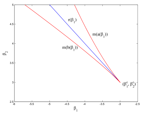
Figure 1. The V-shaped region (with phase transition curve r(β1)𝑟subscript𝛽1r(\beta_{1}) inside) in the (β1,β2)subscript𝛽1subscript𝛽2(\beta_{1},\beta_{2}) plane. Graph drawn for p=2𝑝2p=2.
Proof.

The moment generating function for the uniform (0,1)01(0,1) distribution is given by M(θ)=(eθ1)/θ𝑀𝜃superscript𝑒𝜃1𝜃M(\theta)=(e^{\theta}-1)/\theta. The associated Cramér function I𝐼I is finite on (0,1)01(0,1),

I(u)=supθ(θulogeθ1θ),𝐼𝑢subscriptsupremum𝜃𝜃𝑢superscript𝑒𝜃1𝜃I(u)=\sup_{\theta\in\mathbb{R}}\left(\theta u-\log\frac{e^{\theta}-1}{\theta}\right), (4.3)

but does not admit a closed-form expression. As shown in Theorem 3.4, the limiting normalization constant ψβsuperscriptsubscript𝜓𝛽\psi_{\infty}^{\beta} exists and is given by

ψβ=sup0u1(β1u+β2up12I(u)).superscriptsubscript𝜓𝛽subscriptsupremum0𝑢1subscript𝛽1𝑢subscript𝛽2superscript𝑢𝑝12𝐼𝑢\psi_{\infty}^{\beta}=\sup_{0\leq u\leq 1}\left(\beta_{1}u+\beta_{2}u^{p}-\frac{1}{2}I(u)\right). (4.4)

A significant part of computing phase boundaries for the 222-parameter exponential model is then a detailed analysis of the calculus problem (4.4). However, as straightforward as it sounds, since the exact form of I𝐼I is not obtainable, getting a clear picture of the asymptotic phase structure is not that easy and various tricks need to be employed.

Consider the maximization problem for l(u;β1,β2)=β1u+β2up12I(u)𝑙𝑢subscript𝛽1subscript𝛽2subscript𝛽1𝑢subscript𝛽2superscript𝑢𝑝12𝐼𝑢l(u;\beta_{1},\beta_{2})=\beta_{1}u+\beta_{2}u^{p}-\frac{1}{2}I(u) on the interval [0,1]01[0,1], where <β1<subscript𝛽1-\infty<\beta_{1}<\infty and 0β2<0subscript𝛽20\leq\beta_{2}<\infty are parameters. The location of maximizers of l(u)𝑙𝑢l(u) on the interval [0,1]01[0,1] is closely related to properties of its derivatives l(u)superscript𝑙𝑢l^{\prime}(u) and l′′(u)superscript𝑙′′𝑢l^{\prime\prime}(u),

l(u)=β1+pβ2up112I(u),superscript𝑙𝑢subscript𝛽1𝑝subscript𝛽2superscript𝑢𝑝112superscript𝐼𝑢l^{\prime}(u)=\beta_{1}+p\beta_{2}u^{p-1}-\frac{1}{2}I^{\prime}(u), (4.5)
l′′(u)=p(p1)β2up212I′′(u).superscript𝑙′′𝑢𝑝𝑝1subscript𝛽2superscript𝑢𝑝212superscript𝐼′′𝑢l^{\prime\prime}(u)=p(p-1)\beta_{2}u^{p-2}-\frac{1}{2}I^{\prime\prime}(u).
Refer to caption
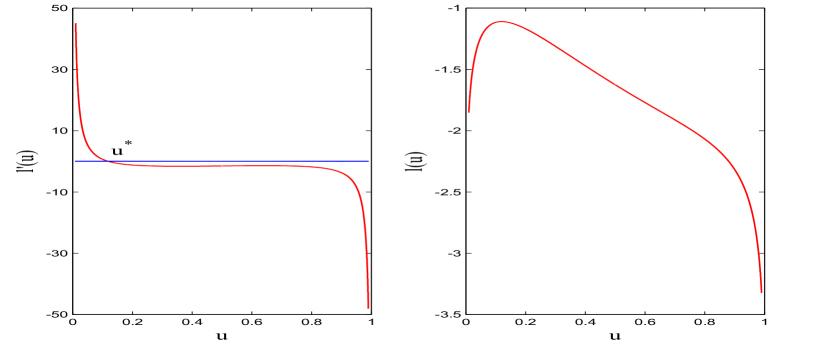
Figure 2. Outside the V-shaped region, l(u)𝑙𝑢l(u) has a unique local maximizer (hence global maximizer) usuperscript𝑢u^{*}. Graph drawn for β1=5subscript𝛽15\beta_{1}=-5, β2=3.5subscript𝛽23.5\beta_{2}=3.5, and p=2𝑝2p=2.

Following the duality principle for the Legendre transform between I(u)𝐼𝑢I(u) and logM(θ)𝑀𝜃\log M(\theta) [36], we first analyze properties of l′′(u)superscript𝑙′′𝑢l^{\prime\prime}(u) on the interval [0,1]01[0,1]. Recall that

I(u)+logeθ1θ=θu,𝐼𝑢superscript𝑒𝜃1𝜃𝜃𝑢I(u)+\log\frac{e^{\theta}-1}{\theta}=\theta u, (4.6)

where θ𝜃\theta and u𝑢u are implicitly related. Taking derivatives, we have

u=(logeθ1θ)|θ,𝑢evaluated-atsuperscript𝑒𝜃1𝜃𝜃u=\left.\left(\log\frac{e^{\theta}-1}{\theta}\right)\right|_{\theta}^{\prime}, (4.7)
I′′(u)(logeθ1θ)|θ′′=1.evaluated-atsuperscript𝐼′′𝑢superscript𝑒𝜃1𝜃𝜃′′1I^{\prime\prime}(u)\cdot\left.\left(\log\frac{e^{\theta}-1}{\theta}\right)\right|_{\theta}^{\prime\prime}=1.

Consider the function

m(u)=I′′(u)2p(p1)up2𝑚𝑢superscript𝐼′′𝑢2𝑝𝑝1superscript𝑢𝑝2m(u)=\frac{I^{\prime\prime}(u)}{2p(p-1)u^{p-2}} (4.8)

on [0,1]01[0,1]. By (4.7), analyzing properties of m(u)𝑚𝑢m(u) translates to analyzing properties of the function

n(θ)𝑛𝜃\displaystyle n(\theta) =\displaystyle= 2p(p1)(logeθ1θ)|θ′′((logeθ1θ)|θ)p2evaluated-at2𝑝𝑝1superscript𝑒𝜃1𝜃𝜃′′superscriptevaluated-atsuperscript𝑒𝜃1𝜃𝜃𝑝2\displaystyle 2p(p-1)\left.\left(\log\frac{e^{\theta}-1}{\theta}\right)\right|_{\theta}^{\prime\prime}\cdot\left(\left.\left(\log\frac{e^{\theta}-1}{\theta}\right)\right|_{\theta}^{\prime}\right)^{p-2}
=\displaystyle= 2p(p1)(e2θeθ(θ2+2)+1(eθ1)2θ2)(eθ(θ1)+1(eθ1)θ)p22𝑝𝑝1superscript𝑒2𝜃superscript𝑒𝜃superscript𝜃221superscriptsuperscript𝑒𝜃12superscript𝜃2superscriptsuperscript𝑒𝜃𝜃11superscript𝑒𝜃1𝜃𝑝2\displaystyle 2p(p-1)\left(\frac{e^{2\theta}-e^{\theta}(\theta^{2}+2)+1}{(e^{\theta}-1)^{2}\theta^{2}}\right)\left(\frac{e^{\theta}(\theta-1)+1}{(e^{\theta}-1)\theta}\right)^{p-2}

over \mathbb{R}, where m(u)n(θ)=1𝑚𝑢𝑛𝜃1m(u)n(\theta)=1 and u𝑢u and θ𝜃\theta satisfy the dual relationship. We recognize that

limθn(θ)=0,subscript𝜃𝑛𝜃0\lim_{\theta\rightarrow-\infty}n(\theta)=0, (4.10)
limθ0n(θ)=p(p1)3(12)p1,subscript𝜃0𝑛𝜃𝑝𝑝13superscript12𝑝1\lim_{\theta\rightarrow 0}n(\theta)=\frac{p(p-1)}{3}\left(\frac{1}{2}\right)^{p-1},
limθn(θ)=0,subscript𝜃𝑛𝜃0\lim_{\theta\rightarrow\infty}n(\theta)=0,

which implies that n(θ)𝑛𝜃n(\theta) achieves a finite global maximum. We claim that the global maximum can only be attained at θ00subscript𝜃00\theta_{0}\geq 0. This would further imply that there is a finite global minimum for m(u)𝑚𝑢m(u), and it can only be attained at u012subscript𝑢012u_{0}\geq\frac{1}{2}. First suppose p=2𝑝2p=2. Then n(θ0)=0superscript𝑛subscript𝜃00n^{\prime}(\theta_{0})=0 easily implies that θ0=0subscript𝜃00\theta_{0}=0. Now suppose p>2𝑝2p>2. Then since n(θ0)=0superscript𝑛subscript𝜃00n^{\prime}(\theta_{0})=0, we have

(e2θeθ(θ2+2)+1(eθ1)2θ2)|θ0(eθ(θ1)+1(eθ1)θ)|θ0=(p2)(e2θeθ(θ2+2)+1(eθ1)2θ2)2|θ0<0.evaluated-atevaluated-atsuperscript𝑒2𝜃superscript𝑒𝜃superscript𝜃221superscriptsuperscript𝑒𝜃12superscript𝜃2subscript𝜃0superscript𝑒𝜃𝜃11superscript𝑒𝜃1𝜃subscript𝜃0evaluated-at𝑝2superscriptsuperscript𝑒2𝜃superscript𝑒𝜃superscript𝜃221superscriptsuperscript𝑒𝜃12superscript𝜃22subscript𝜃00\left.\left(\frac{e^{2\theta}-e^{\theta}(\theta^{2}+2)+1}{(e^{\theta}-1)^{2}\theta^{2}}\right)\right|_{\theta_{0}}^{\prime}\left.\left(\frac{e^{\theta}(\theta-1)+1}{(e^{\theta}-1)\theta}\right)\right|_{\theta_{0}}=-(p-2)\left.\left(\frac{e^{2\theta}-e^{\theta}(\theta^{2}+2)+1}{(e^{\theta}-1)^{2}\theta^{2}}\right)^{2}\right|_{\theta_{0}}<0. (4.11)

This says that θ0subscript𝜃0\theta_{0} is on the portion of \mathbb{R} where (e2θeθ(θ2+2)+1)/((eθ1)2θ2)superscript𝑒2𝜃superscript𝑒𝜃superscript𝜃221superscriptsuperscript𝑒𝜃12superscript𝜃2\left(e^{2\theta}-e^{\theta}(\theta^{2}+2)+1\right)/\left((e^{\theta}-1)^{2}\theta^{2}\right) is decreasing, i.e., θ0>0subscript𝜃00\theta_{0}>0. As θ𝜃\theta goes from 00 to \infty, the left hand side of (4.11) first decreases from 00 then increases to 00 and is always negative, whereas the right hand side of (4.11) monotonically increases from (p2)/144𝑝2144-(p-2)/144 to 00 and approaches 00 at a rate faster than the left hand side, and so there exists a θ0subscript𝜃0\theta_{0} which makes both sides equal. Our numerical computations show that n(θ0)=0superscript𝑛subscript𝜃00n^{\prime}(\theta_{0})=0 is uniquely defined, and n(θ)𝑛𝜃n(\theta) increases from -\infty to θ0subscript𝜃0\theta_{0} and decreases from θ0subscript𝜃0\theta_{0} to \infty. See Table 1 for some of these critical values.

p𝑝p θ0subscript𝜃0\theta_{0} n(θ0)𝑛subscript𝜃0n(\theta_{0}) u0subscript𝑢0u_{0} m(u0)𝑚subscript𝑢0m(u_{0})
222 00 0.33330.33330.3333 0.50.50.5 333
333 1.32511.32511.3251 0.55750.55750.5575 0.60730.60730.6073 1.79371.79371.7937
555 2.98692.98692.9869 0.83240.83240.8324 0.71830.71830.7183 1.20141.20141.2014
101010 5.62565.62565.6256 1.08941.08941.0894 0.82590.82590.8259 0.91800.91800.9180
Table 1. Critical values for m(u)𝑚𝑢m(u) and n(θ)𝑛𝜃n(\theta) as a function of p𝑝p.

The above analysis shows that for β2m(u0)subscript𝛽2𝑚subscript𝑢0\beta_{2}\leq m(u_{0}), l′′(u)0superscript𝑙′′𝑢0l^{\prime\prime}(u)\leq 0 over the entire interval [0,1]01[0,1]; while for β2>m(u0)subscript𝛽2𝑚subscript𝑢0\beta_{2}>m(u_{0}), l′′(u)superscript𝑙′′𝑢l^{\prime\prime}(u) takes on both positive and negative values, and we denote the transition points by u1subscript𝑢1u_{1} and u2subscript𝑢2u_{2} (u1<u0<u2subscript𝑢1subscript𝑢0subscript𝑢2u_{1}<u_{0}<u_{2}). Properties of l′′(u)superscript𝑙′′𝑢l^{\prime\prime}(u) on [0,1]01[0,1] entails properties of l(u)superscript𝑙𝑢l^{\prime}(u) over the same interval. For β2m(u0)subscript𝛽2𝑚subscript𝑢0\beta_{2}\leq m(u_{0}), l(u)superscript𝑙𝑢l^{\prime}(u) is monotonically decreasing. For β2>m(u0)subscript𝛽2𝑚subscript𝑢0\beta_{2}>m(u_{0}), l(u)superscript𝑙𝑢l^{\prime}(u) is decreasing from 00 to u1subscript𝑢1u_{1}, increasing from u1subscript𝑢1u_{1} to u2subscript𝑢2u_{2}, and then decreasing again from u2subscript𝑢2u_{2} to 111.

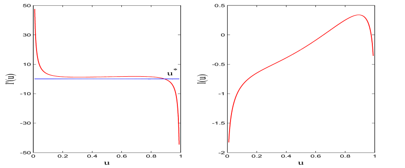
The analytic properties of l′′(u)superscript𝑙′′𝑢l^{\prime\prime}(u) and l(u)superscript𝑙𝑢l^{\prime}(u) help us investigate properties of l(u)𝑙𝑢l(u) on the interval [0,1]01[0,1]. Being the Legendre transform of a smooth function, I(u)𝐼𝑢I(u) is a smooth function, and grows unbounded when u𝑢u approaches 00 or 111. By the duality principle for the Legendre transform, I(u)=θsuperscript𝐼𝑢𝜃I^{\prime}(u)=\theta where θ𝜃\theta and u𝑢u are linked through (4.7), so I(0)=superscript𝐼0I^{\prime}(0)=-\infty and I(1)=superscript𝐼1I^{\prime}(1)=\infty. This says that l(u)𝑙𝑢l(u) is a smooth function, l(0)=l(1)=𝑙0𝑙1l(0)=l(1)=-\infty, l(0)=superscript𝑙0l^{\prime}(0)=\infty and l(1)=superscript𝑙1l^{\prime}(1)=-\infty, so l(u)𝑙𝑢l(u) can not be maximized at 00 or 111. For β2m(u0)subscript𝛽2𝑚subscript𝑢0\beta_{2}\leq m(u_{0}), l(u)superscript𝑙𝑢l^{\prime}(u) crosses the u𝑢u-axis only once, going from positive to negative. Thus l(u)𝑙𝑢l(u) has a unique local maximizer (hence global maximizer) usuperscript𝑢u^{*}. For β2>m(u0)subscript𝛽2𝑚subscript𝑢0\beta_{2}>m(u_{0}), the situation is more complicated. If l(u1)0superscript𝑙subscript𝑢10l^{\prime}(u_{1})\geq 0 (resp. l(u2)0superscript𝑙subscript𝑢20l^{\prime}(u_{2})\leq 0), l(u)𝑙𝑢l(u) has a unique local maximizer (hence global maximizer) at a point u>u2superscript𝑢subscript𝑢2u^{*}>u_{2} (resp. u<u1superscript𝑢subscript𝑢1u^{*}<u_{1}). See Figures 2 and 3. If l(u1)<0<l(u2)superscript𝑙subscript𝑢10superscript𝑙subscript𝑢2l^{\prime}(u_{1})<0<l^{\prime}(u_{2}), then l(u)𝑙𝑢l(u) has two local maximizers u1superscriptsubscript𝑢1u_{1}^{*} and u2superscriptsubscript𝑢2u_{2}^{*}, with u1<u1<u0<u2<u2superscriptsubscript𝑢1subscript𝑢1subscript𝑢0subscript𝑢2superscriptsubscript𝑢2u_{1}^{*}<u_{1}<u_{0}<u_{2}<u_{2}^{*}.

Refer to caption
Figure 3. Outside the V-shaped region, l(u)𝑙𝑢l(u) has a unique local maximizer (hence global maximizer) usuperscript𝑢u^{*}. Graph drawn for β1=2.5subscript𝛽12.5\beta_{1}=-2.5, β2=4subscript𝛽24\beta_{2}=4, and p=2𝑝2p=2.

Let

f(u)=uI′′(u)2(p1)12I(u)𝑓𝑢𝑢superscript𝐼′′𝑢2𝑝112superscript𝐼𝑢f(u)=\frac{uI^{\prime\prime}(u)}{2(p-1)}-\frac{1}{2}I^{\prime}(u) (4.12)

so that l(u1)=β1+f(u1)superscript𝑙subscript𝑢1subscript𝛽1𝑓subscript𝑢1l^{\prime}(u_{1})=\beta_{1}+f(u_{1}) and l(u2)=β1+f(u2)superscript𝑙subscript𝑢2subscript𝛽1𝑓subscript𝑢2l^{\prime}(u_{2})=\beta_{1}+f(u_{2}). Again by the duality principle for the Legendre transform, analyzing properties of the function f(u)𝑓𝑢f(u) on [0,1]01[0,1] translates to analyzing properties of the function

g(θ)=θ(eθ1)(eθ(θ1)+1)2(p1)(e2θeθ(θ2+2)+1)12θ𝑔𝜃𝜃superscript𝑒𝜃1superscript𝑒𝜃𝜃112𝑝1superscript𝑒2𝜃superscript𝑒𝜃superscript𝜃22112𝜃g(\theta)=\frac{\theta\left(e^{\theta}-1\right)\left(e^{\theta}(\theta-1)+1\right)}{2(p-1)\left(e^{2\theta}-e^{\theta}(\theta^{2}+2)+1\right)}-\frac{1}{2}\theta (4.13)

over \mathbb{R}, where f(u)=g(θ)𝑓𝑢𝑔𝜃f(u)=g(\theta) and u𝑢u and θ𝜃\theta satisfy the dual relationship. We recognize that

limθg(θ)=,subscript𝜃𝑔𝜃\lim_{\theta\rightarrow-\infty}g(\theta)=\infty, (4.14)
limθ0g(θ)=3p1,subscript𝜃0𝑔𝜃3𝑝1\lim_{\theta\rightarrow 0}g(\theta)=\frac{3}{p-1},
limθg(θ)=,subscript𝜃𝑔𝜃\lim_{\theta\rightarrow\infty}g(\theta)=\infty,

which implies that g(θ)𝑔𝜃g(\theta) achieves a finite global minimum. We claim that the global minimum can only be attained at the same unique θ0subscript𝜃0\theta_{0} that makes n(θ)=0superscript𝑛𝜃0n^{\prime}(\theta)=0. This can be checked by identifying the condition for g(θ)=0superscript𝑔𝜃0g^{\prime}(\theta)=0. For p=2𝑝2p=2, g(θ0)=0superscript𝑔subscript𝜃00g^{\prime}(\theta_{0})=0 easily implies that θ0=0subscript𝜃00\theta_{0}=0. For p>2𝑝2p>2, since g(θ0)=0superscript𝑔subscript𝜃00g^{\prime}(\theta_{0})=0, we have

(eθ(θ1)+1(eθ1)θ)|θ0(e2θeθ(θ2+2)+1(eθ1)2θ2)|θ0(e2θeθ(θ2+2)+1(eθ1)2θ2)|θ0(eθ(θ1)+1(eθ1)θ)|θ0=(p1)(e2θeθ(θ2+2)+1(eθ1)2θ2)2|θ0,evaluated-atevaluated-atsuperscript𝑒𝜃𝜃11superscript𝑒𝜃1𝜃subscript𝜃0superscript𝑒2𝜃superscript𝑒𝜃superscript𝜃221superscriptsuperscript𝑒𝜃12superscript𝜃2subscript𝜃0evaluated-atevaluated-atsuperscript𝑒2𝜃superscript𝑒𝜃superscript𝜃221superscriptsuperscript𝑒𝜃12superscript𝜃2subscript𝜃0superscript𝑒𝜃𝜃11superscript𝑒𝜃1𝜃subscript𝜃0evaluated-at𝑝1superscriptsuperscript𝑒2𝜃superscript𝑒𝜃superscript𝜃221superscriptsuperscript𝑒𝜃12superscript𝜃22subscript𝜃0\left.\left(\frac{e^{\theta}(\theta-1)+1}{(e^{\theta}-1)\theta}\right)\right|_{\theta_{0}}^{\prime}\left.\left(\frac{e^{2\theta}-e^{\theta}(\theta^{2}+2)+1}{(e^{\theta}-1)^{2}\theta^{2}}\right)\right|_{\theta_{0}}-\left.\left(\frac{e^{2\theta}-e^{\theta}(\theta^{2}+2)+1}{(e^{\theta}-1)^{2}\theta^{2}}\right)\right|_{\theta_{0}}^{\prime}\left.\left(\frac{e^{\theta}(\theta-1)+1}{(e^{\theta}-1)\theta}\right)\right|_{\theta_{0}}\\ =(p-1)\left.\left(\frac{e^{2\theta}-e^{\theta}(\theta^{2}+2)+1}{(e^{\theta}-1)^{2}\theta^{2}}\right)^{2}\right|_{\theta_{0}}, (4.15)

which yields the same solution as (4.11) after a simple transformation. Thus g(θ)𝑔𝜃g(\theta) decreases from -\infty to θ0subscript𝜃0\theta_{0} and increases from θ0subscript𝜃0\theta_{0} to \infty. This further implies that there is a finite global minimum for f(u)𝑓𝑢f(u) attained at u0subscript𝑢0u_{0}, and f(u)𝑓𝑢f(u) decreases from 00 to u0subscript𝑢0u_{0} and increases from u0subscript𝑢0u_{0} to 111. Both θ0subscript𝜃0\theta_{0} and u0subscript𝑢0u_{0} coincide with the critical values listed in Table 1. See Table 2. We conclude that l(u1)0superscript𝑙subscript𝑢10l^{\prime}(u_{1})\geq 0 for β1f(u0)subscript𝛽1𝑓subscript𝑢0\beta_{1}\geq-f(u_{0}) and β2=m(u0)subscript𝛽2𝑚subscript𝑢0\beta_{2}=m(u_{0}). The only possible region in the (β1,β2)subscript𝛽1subscript𝛽2(\beta_{1},\beta_{2}) plane where l(u1)<0<l(u2)superscript𝑙subscript𝑢10superscript𝑙subscript𝑢2l^{\prime}(u_{1})<0<l^{\prime}(u_{2}) is bounded by β1<f(u0):=β1csubscript𝛽1𝑓subscript𝑢0assignsuperscriptsubscript𝛽1𝑐\beta_{1}<-f(u_{0}):=\beta_{1}^{c} and β2>m(u0):=β2csubscript𝛽2𝑚subscript𝑢0assignsuperscriptsubscript𝛽2𝑐\beta_{2}>m(u_{0}):=\beta_{2}^{c}.

p𝑝p θ0subscript𝜃0\theta_{0} g(θ0)𝑔subscript𝜃0g(\theta_{0}) u0subscript𝑢0u_{0} f(u0)𝑓subscript𝑢0f(u_{0})
222 00 333 0.50.50.5 333
333 1.32511.32511.3251 1.32221.32221.3222 0.60730.60730.6073 1.32221.32221.3222
555 2.98692.98692.9869 0.10590.10590.1059 0.71830.71830.7183 0.10590.10590.1059
101010 5.62565.62565.6256 1.17231.1723-1.1723 0.82590.82590.8259 1.17231.1723-1.1723
Table 2. Critical values for f(u)𝑓𝑢f(u) and g(θ)𝑔𝜃g(\theta) as a function of p𝑝p.

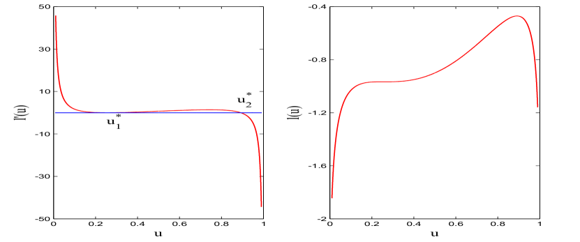
We examine the behavior of l(u1)superscript𝑙subscript𝑢1l^{\prime}(u_{1}) and l(u2)superscript𝑙subscript𝑢2l^{\prime}(u_{2}) more closely when β1subscript𝛽1\beta_{1} and β2subscript𝛽2\beta_{2} are chosen from this region. Recall that u1<u0<u2subscript𝑢1subscript𝑢0subscript𝑢2u_{1}<u_{0}<u_{2}. By monotonicity of f(u)𝑓𝑢f(u) on the intervals (0,u0)0subscript𝑢0(0,u_{0}) and (u0,1)subscript𝑢01(u_{0},1), there exist continuous functions a(β1)𝑎subscript𝛽1a(\beta_{1}) and b(β1)𝑏subscript𝛽1b(\beta_{1}) of β1subscript𝛽1\beta_{1}, such that l(u1)<0superscript𝑙subscript𝑢10l^{\prime}(u_{1})<0 for u1>a(β1)subscript𝑢1𝑎subscript𝛽1u_{1}>a(\beta_{1}) and l(u2)>0superscript𝑙subscript𝑢20l^{\prime}(u_{2})>0 for u2>b(β1)subscript𝑢2𝑏subscript𝛽1u_{2}>b(\beta_{1}). As β1subscript𝛽1\beta_{1}\rightarrow-\infty, a(β1)0𝑎subscript𝛽10a(\beta_{1})\rightarrow 0 and b(β1)1𝑏subscript𝛽11b(\beta_{1})\rightarrow 1. a(β1)𝑎subscript𝛽1a(\beta_{1}) is an increasing function of β1subscript𝛽1\beta_{1}, whereas b(β1)𝑏subscript𝛽1b(\beta_{1}) is a decreasing function, and they satisfy f(a(β1))=f(b(β1))=β1𝑓𝑎subscript𝛽1𝑓𝑏subscript𝛽1subscript𝛽1f(a(\beta_{1}))=f(b(\beta_{1}))=-\beta_{1}. The restrictions on u1subscript𝑢1u_{1} and u2subscript𝑢2u_{2} yield restrictions on β2subscript𝛽2\beta_{2}, and we have l(u1)<0superscript𝑙subscript𝑢10l^{\prime}(u_{1})<0 for β2<m(a(β1))subscript𝛽2𝑚𝑎subscript𝛽1\beta_{2}<m(a(\beta_{1})) and l(u2)>0superscript𝑙subscript𝑢20l^{\prime}(u_{2})>0 for β2>m(b(β1))subscript𝛽2𝑚𝑏subscript𝛽1\beta_{2}>m(b(\beta_{1})). As β1subscript𝛽1\beta_{1}\rightarrow-\infty, m(a(β1))𝑚𝑎subscript𝛽1m(a(\beta_{1}))\rightarrow\infty and m(b(β1))𝑚𝑏subscript𝛽1m(b(\beta_{1}))\rightarrow\infty. m(a(β1))𝑚𝑎subscript𝛽1m(a(\beta_{1})) and m(b(β1))𝑚𝑏subscript𝛽1m(b(\beta_{1})) are both decreasing functions of β1subscript𝛽1\beta_{1}, and they satisfy l(u1)=0superscript𝑙subscript𝑢10l^{\prime}(u_{1})=0 when β2=m(a(β1))subscript𝛽2𝑚𝑎subscript𝛽1\beta_{2}=m(a(\beta_{1})) and l(u2)=0superscript𝑙subscript𝑢20l^{\prime}(u_{2})=0 when β2=m(b(β1))subscript𝛽2𝑚𝑏subscript𝛽1\beta_{2}=m(b(\beta_{1})). As l(u2)>l(u1)superscript𝑙subscript𝑢2superscript𝑙subscript𝑢1l^{\prime}(u_{2})>l^{\prime}(u_{1}) for every (β1,β2)subscript𝛽1subscript𝛽2(\beta_{1},\beta_{2}), the curve m(b(β1))𝑚𝑏subscript𝛽1m(b(\beta_{1})) must lie below the curve m(a(β1))𝑚𝑎subscript𝛽1m(a(\beta_{1})), and together they generate the bounding curves of the V𝑉V-shaped region in the (β1,β2)subscript𝛽1subscript𝛽2(\beta_{1},\beta_{2}) plane with corner point (β1c,β2c)superscriptsubscript𝛽1𝑐superscriptsubscript𝛽2𝑐(\beta_{1}^{c},\beta_{2}^{c}) where two local maximizers exist for l(u)𝑙𝑢l(u). See Figures 1, 4 and 5.

Refer to caption
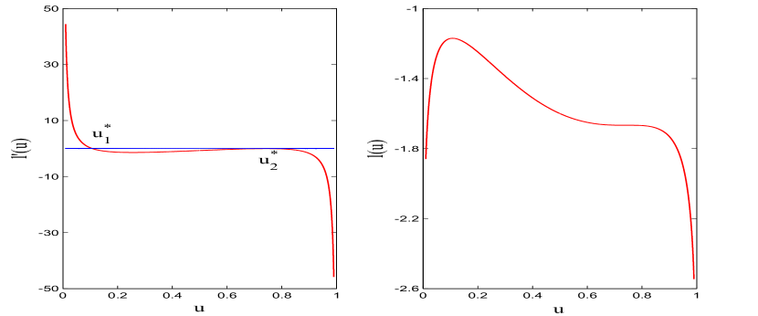
Figure 4. Along the lower bounding curve m(b(β1))𝑚𝑏subscript𝛽1m(b(\beta_{1})) of the V-shaped region, l(u)superscript𝑙𝑢l^{\prime}(u) has two zeros u1superscriptsubscript𝑢1u_{1}^{*} and u2superscriptsubscript𝑢2u_{2}^{*}, but only u1superscriptsubscript𝑢1u_{1}^{*} is the global maximizer for l(u)𝑙𝑢l(u). Graph drawn for β1=5.7subscript𝛽15.7\beta_{1}=-5.7, β2=5subscript𝛽25\beta_{2}=5, and p=2𝑝2p=2.

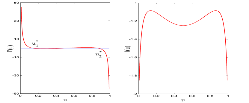
Fix an arbitrary β1<β1csubscript𝛽1superscriptsubscript𝛽1𝑐\beta_{1}<\beta_{1}^{c}, we examine the effect of varying β2subscript𝛽2\beta_{2} on the graph of l(u)superscript𝑙𝑢l^{\prime}(u). It is clear that l(u)superscript𝑙𝑢l^{\prime}(u) shifts upward as β2subscript𝛽2\beta_{2} increases and downward as β2subscript𝛽2\beta_{2} decreases. As a result, as β2subscript𝛽2\beta_{2} gets large, the positive area bounded by the curve l(u)superscript𝑙𝑢l^{\prime}(u) increases, whereas the negative area decreases. By the fundamental theorem of calculus, the difference between the positive and negative areas is the difference between l(u2)𝑙superscriptsubscript𝑢2l(u_{2}^{*}) and l(u1)𝑙superscriptsubscript𝑢1l(u_{1}^{*}), which goes from negative (l(u2)=0superscript𝑙subscript𝑢20l^{\prime}(u_{2})=0, u1superscriptsubscript𝑢1u_{1}^{*} is the global maximizer) to positive (l(u1)=0superscript𝑙subscript𝑢10l^{\prime}(u_{1})=0, u2superscriptsubscript𝑢2u_{2}^{*} is the global maximizer) as β2subscript𝛽2\beta_{2} goes from m(b(β1))𝑚𝑏subscript𝛽1m(b(\beta_{1})) to m(a(β1))𝑚𝑎subscript𝛽1m(a(\beta_{1})). Thus there must be a unique β2subscript𝛽2\beta_{2}: m(b(β1))<β2<m(a(β1))𝑚𝑏subscript𝛽1subscript𝛽2𝑚𝑎subscript𝛽1m(b(\beta_{1}))<\beta_{2}<m(a(\beta_{1})) such that u1superscriptsubscript𝑢1u_{1}^{*} and u2superscriptsubscript𝑢2u_{2}^{*} are both global maximizers, and we denote this β2subscript𝛽2\beta_{2} by r(β1)𝑟subscript𝛽1r(\beta_{1}). See Figures 1 and 6. The parameter values of (β1,r(β1))subscript𝛽1𝑟subscript𝛽1(\beta_{1},r(\beta_{1})) are exactly the ones for which positive and negative areas bounded by l(u)superscript𝑙𝑢l^{\prime}(u) equal each other. An increase in β1subscript𝛽1\beta_{1} induces an upward shift of l(u)superscript𝑙𝑢l^{\prime}(u), and may be balanced by a decrease in β2subscript𝛽2\beta_{2}. Similarly, a decrease in β1subscript𝛽1\beta_{1} induces a downward shift of l(u)superscript𝑙𝑢l^{\prime}(u), and may be balanced by an increase in β2subscript𝛽2\beta_{2}. This justifies that r(β1)𝑟subscript𝛽1r(\beta_{1}) is monotonically decreasing in β1subscript𝛽1\beta_{1}.

The rest of the proof follows as in the proof of the corresponding result (Theorem 2.1) in Radin and Yin [30], where some probability estimates were used. A (jump) discontinuity in the first derivatives of ψβsuperscriptsubscript𝜓𝛽\psi_{\infty}^{\beta} across the curve β2=r(β1)subscript𝛽2𝑟subscript𝛽1\beta_{2}=r(\beta_{1}) indicates a discontinuity in the expected local densities (2.6), while the divergence of the second derivatives of ψβsuperscriptsubscript𝜓𝛽\psi_{\infty}^{\beta} at the critical point (β1c,β2c)superscriptsubscript𝛽1𝑐superscriptsubscript𝛽2𝑐(\beta_{1}^{c},\beta_{2}^{c}) implies that the covariances of the local densities go to zero more slowly than 1/n21superscript𝑛21/n^{2} (2.7). We omit the proof details. ∎

Remark.

The maximization problem (4.4) is solved at a unique value usuperscript𝑢u^{*} off the phase transition curve β2=r(β1)subscript𝛽2𝑟subscript𝛽1\beta_{2}=r(\beta_{1}), and at two values u1superscriptsubscript𝑢1u_{1}^{*} and u2superscriptsubscript𝑢2u_{2}^{*} along the curve. As β1subscript𝛽1\beta_{1}\rightarrow-\infty (resp. β2subscript𝛽2\beta_{2}\rightarrow\infty), u10superscriptsubscript𝑢10u_{1}^{*}\rightarrow 0 and u21superscriptsubscript𝑢21u_{2}^{*}\rightarrow 1. The jump from u1superscriptsubscript𝑢1u_{1}^{*} to u2superscriptsubscript𝑢2u_{2}^{*} is quite noticeable even for small parameter values of β𝛽\beta. For example, taking p=2𝑝2p=2, β1=5subscript𝛽15\beta_{1}=-5, and β2=5subscript𝛽25\beta_{2}=5, numerical computations yield that u10.137superscriptsubscript𝑢10.137u_{1}^{*}\approx 0.137 and u20.863superscriptsubscript𝑢20.863u_{2}^{*}\approx 0.863 with l(u1)l(u2)1.0854𝑙superscriptsubscript𝑢1𝑙superscriptsubscript𝑢21.0854l(u_{1}^{*})\approx l(u_{2}^{*})\approx-1.0854.

Refer to caption
Figure 5. Along the upper bounding curve m(a(β1))𝑚𝑎subscript𝛽1m(a(\beta_{1})) of the V-shaped region, l(u)superscript𝑙𝑢l^{\prime}(u) has two zeros u1superscriptsubscript𝑢1u_{1}^{*} and u2superscriptsubscript𝑢2u_{2}^{*}, but only u2superscriptsubscript𝑢2u_{2}^{*} is the global maximizer for l(u)𝑙𝑢l(u). Graph drawn for β1=4.3subscript𝛽14.3\beta_{1}=-4.3, β2=5subscript𝛽25\beta_{2}=5, and p=2𝑝2p=2.
Proposition 4.3.

The Cramér function I(u)𝐼𝑢I(u) (4.3) for the uniform distribution on (0,1)01(0,1) is symmetric about the line u=12𝑢12u=\frac{1}{2}.

Proof.

Recall that I(u)𝐼𝑢I(u) is the Legendre transform of the log moment generating function logM(θ)𝑀𝜃\log M(\theta) for the uniform (0,1)01(0,1) distribution. Take 0<u<120𝑢120<u<\frac{1}{2}. Though the exact form of I𝐼I is not obtainable, following the duality principle, we have

I(u)=θ1ulogeθ11θ1,𝐼𝑢subscript𝜃1𝑢superscript𝑒subscript𝜃11subscript𝜃1I(u)=\theta_{1}u-\log\frac{e^{\theta_{1}}-1}{\theta_{1}}, (4.16)
I(1u)=θ2(1u)logeθ21θ2,𝐼1𝑢subscript𝜃21𝑢superscript𝑒subscript𝜃21subscript𝜃2I(1-u)=\theta_{2}(1-u)-\log\frac{e^{\theta_{2}}-1}{\theta_{2}},

where θ1subscript𝜃1\theta_{1} and θ2subscript𝜃2\theta_{2} are both finite and uniquely defined, and satisfy I(u)=θ1superscript𝐼𝑢subscript𝜃1I^{\prime}(u)=\theta_{1} and I(1u)=θ2superscript𝐼1𝑢subscript𝜃2I^{\prime}(1-u)=\theta_{2}. We show that I(u)=I(1u)𝐼𝑢𝐼1𝑢I(u)=I(1-u) when θ2=θ1subscript𝜃2subscript𝜃1\theta_{2}=-\theta_{1}. The calculation is straightforward:

I(1u)=θ1(1u)logeθ11θ1=θ1ulogeθ11θ1=I(u).𝐼1𝑢subscript𝜃11𝑢superscript𝑒subscript𝜃11subscript𝜃1subscript𝜃1𝑢superscript𝑒subscript𝜃11subscript𝜃1𝐼𝑢I(1-u)=-\theta_{1}(1-u)-\log\frac{e^{-\theta_{1}}-1}{-\theta_{1}}=\theta_{1}u-\log\frac{e^{\theta_{1}}-1}{\theta_{1}}=I(u). (4.17)

This verifies our claim. ∎

Corollary 4.4.

Take H1subscript𝐻1H_{1} a single edge and H2subscript𝐻2H_{2} a finite simple graph with p2𝑝2p\geq 2 edges. The associated phase transition curve β2=r(β1)subscript𝛽2𝑟subscript𝛽1\beta_{2}=r(\beta_{1}) lies above the straight line β2=β1subscript𝛽2subscript𝛽1\beta_{2}=-\beta_{1} when p3𝑝3p\geq 3, and is exactly portion of the straight line β2=β1subscript𝛽2subscript𝛽1\beta_{2}=-\beta_{1} (β13subscript𝛽13\beta_{1}\leq-3) when p=2𝑝2p=2.

Proof.

From the proof of Theorem 4.1, there are two global maximizers u1superscriptsubscript𝑢1u_{1}^{*} and u2superscriptsubscript𝑢2u_{2}^{*} for l(u)𝑙𝑢l(u) along the phase transition curve β2=r(β1)subscript𝛽2𝑟subscript𝛽1\beta_{2}=r(\beta_{1}), with u012subscript𝑢012u_{0}\geq\frac{1}{2} and 0<u1<u0<u2<10superscriptsubscript𝑢1subscript𝑢0superscriptsubscript𝑢210<u_{1}^{*}<u_{0}<u_{2}^{*}<1. Furthermore, the y𝑦y-coordinate β2csuperscriptsubscript𝛽2𝑐\beta_{2}^{c} of the critical point (β1c,β2c)superscriptsubscript𝛽1𝑐superscriptsubscript𝛽2𝑐(\beta_{1}^{c},\beta_{2}^{c}) is always positive. On the straight line β1+β2=0subscript𝛽1subscript𝛽20\beta_{1}+\beta_{2}=0, we rewrite l(u)=β1(uup)12I(u)𝑙𝑢subscript𝛽1𝑢superscript𝑢𝑝12𝐼𝑢l(u)=\beta_{1}(u-u^{p})-\frac{1}{2}I(u). First suppose p=2𝑝2p=2. Since I(u)𝐼𝑢I(u) and uu2𝑢superscript𝑢2u-u^{2} are both symmetric about the line u=12𝑢12u=\frac{1}{2}, two global maximizers u1superscriptsubscript𝑢1u_{1}^{*} and u2superscriptsubscript𝑢2u_{2}^{*} exist for l(u)𝑙𝑢l(u). Next consider the generic case p>2𝑝2p>2. Analytical calculations give that uup<(1u)(1u)p𝑢superscript𝑢𝑝1𝑢superscript1𝑢𝑝u-u^{p}<(1-u)-(1-u)^{p} for 0<u<120𝑢120<u<\frac{1}{2}. Since I(u)𝐼𝑢I(u) is symmetric, this says that for β1<0subscript𝛽10\beta_{1}<0 (resp. β2>0subscript𝛽20\beta_{2}>0), the global maximizer usuperscript𝑢u^{*} of l(u)𝑙𝑢l(u) satisfies u12superscript𝑢12u^{*}\leq\frac{1}{2}. This implies the desired result. ∎

Refer to caption
Figure 6. Along the phase transition curve r(β1)𝑟subscript𝛽1r(\beta_{1}), l(u)𝑙𝑢l(u) has two local maximizers u1superscriptsubscript𝑢1u_{1}^{*} and u2superscriptsubscript𝑢2u_{2}^{*}, and both are global maximizers for l(u)𝑙𝑢l(u). Graph drawn for β1=5subscript𝛽15\beta_{1}=-5, β2=5subscript𝛽25\beta_{2}=5, and p=2𝑝2p=2.

5. Further discussion

But what if the common distribution μ𝜇\mu on the edge weights does not have finite support? Unfortunately, we do not have a generic large deviation principle in this case. As an example, we will examine the asymptotic phase structure for a completely solvable exponential model and hope the analysis would provide some inspiration. Let Gn𝒢nsubscript𝐺𝑛subscript𝒢𝑛G_{n}\in\mathcal{G}_{n} be an edge-weighted directed labeled graph on n𝑛n vertices, where the edge weights xijsubscript𝑥𝑖𝑗x_{ij} from vertex i𝑖i to vertex j𝑗j are iid real random variables whose common distribution μ𝜇\mu is standard Gaussian. As in the undirected case, the common distribution for the edge weights yields probability measure nsubscript𝑛\mathbb{P}_{n} and the associated expectation 𝔼nsubscript𝔼𝑛\mathbb{E}_{n} on 𝒢nsubscript𝒢𝑛\mathcal{G}_{n}. Give the set of such graphs the probability

nβ(Gn)=exp(n2(β1e(Gn)+β2s(Gn)ψnβ))n(Gn),superscriptsubscript𝑛𝛽subscript𝐺𝑛superscript𝑛2subscript𝛽1𝑒subscript𝐺𝑛subscript𝛽2𝑠subscript𝐺𝑛superscriptsubscript𝜓𝑛𝛽subscript𝑛subscript𝐺𝑛\mathbb{P}_{n}^{\beta}(G_{n})=\exp\left(n^{2}\left(\beta_{1}e(G_{n})+\beta_{2}s(G_{n})-\psi_{n}^{\beta}\right)\right)\mathbb{P}_{n}(G_{n}), (5.1)

where β=(β1,β2)𝛽subscript𝛽1subscript𝛽2\beta=(\beta_{1},\beta_{2}) are 222 real parameters, H1subscript𝐻1H_{1} is a directed edge, H2subscript𝐻2H_{2} is a directed 222-star, e(Gn)𝑒subscript𝐺𝑛e(G_{n}) and s(Gn)𝑠subscript𝐺𝑛s(G_{n}) are respectively the directed edge and 222-star homomorphism densities of Gnsubscript𝐺𝑛G_{n},

e(Gn)=1n21i,jnxij,s(Gn)=1n31i,j,knxijxik,formulae-sequence𝑒subscript𝐺𝑛1superscript𝑛2subscriptformulae-sequence1𝑖𝑗𝑛subscript𝑥𝑖𝑗𝑠subscript𝐺𝑛1superscript𝑛3subscriptformulae-sequence1𝑖𝑗𝑘𝑛subscript𝑥𝑖𝑗subscript𝑥𝑖𝑘e(G_{n})=\frac{1}{n^{2}}\sum_{1\leq i,j\leq n}x_{ij},\hskip 5.69046pts(G_{n})=\frac{1}{n^{3}}\sum_{1\leq i,j,k\leq n}x_{ij}x_{ik}, (5.2)

and ψnβsuperscriptsubscript𝜓𝑛𝛽\psi_{n}^{\beta} is the normalization constant,

ψnβ=1n2log𝔼n(exp(n2(β1e(Gn)+β2s(Gn)))).superscriptsubscript𝜓𝑛𝛽1superscript𝑛2subscript𝔼𝑛superscript𝑛2subscript𝛽1𝑒subscript𝐺𝑛subscript𝛽2𝑠subscript𝐺𝑛\psi_{n}^{\beta}=\frac{1}{n^{2}}\log\mathbb{E}_{n}\left(\exp\left(n^{2}\left(\beta_{1}e(G_{n})+\beta_{2}s(G_{n})\right)\right)\right). (5.3)

The associated expectation 𝔼nβsuperscriptsubscript𝔼𝑛𝛽\mathbb{E}_{n}^{\beta} may be defined accordingly, and a phase transition occurs when the limiting normalization constant ψβ=limnψnβsubscriptsuperscript𝜓𝛽subscript𝑛superscriptsubscript𝜓𝑛𝛽\displaystyle\psi^{\beta}_{\infty}=\lim_{n\to\infty}\psi_{n}^{\beta} has a singular point.

Plugging the formulas for e(Gn)𝑒subscript𝐺𝑛e(G_{n}) and s(Gn)𝑠subscript𝐺𝑛s(G_{n}) into (5.3) and using the iid property of the edge weights, we have

ψnβsuperscriptsubscript𝜓𝑛𝛽\displaystyle\psi_{n}^{\beta} =\displaystyle= 1n2log𝔼n(exp(β1i=1n(j=1nxij)+β2ni=1n(j=1nxij)2))1superscript𝑛2subscript𝔼𝑛subscript𝛽1superscriptsubscript𝑖1𝑛superscriptsubscript𝑗1𝑛subscript𝑥𝑖𝑗subscript𝛽2𝑛superscriptsubscript𝑖1𝑛superscriptsuperscriptsubscript𝑗1𝑛subscript𝑥𝑖𝑗2\displaystyle\frac{1}{n^{2}}\log\mathbb{E}_{n}\left(\exp\left(\beta_{1}\sum_{i=1}^{n}\left(\sum_{j=1}^{n}x_{ij}\right)+\frac{\beta_{2}}{n}\sum_{i=1}^{n}\left(\sum_{j=1}^{n}x_{ij}\right)^{2}\right)\right)
=\displaystyle= 1nlog𝔼(exp(β1Y+β2nY2)),1𝑛𝔼subscript𝛽1𝑌subscript𝛽2𝑛superscript𝑌2\displaystyle\frac{1}{n}\log\mathbb{E}\left(\exp\left(\beta_{1}Y+\frac{\beta_{2}}{n}Y^{2}\right)\right),

where Y=j=1nx1j𝑌superscriptsubscript𝑗1𝑛subscript𝑥1𝑗Y=\sum_{j=1}^{n}x_{1j} satisfies a Gaussian distribution with mean 00 and variance n𝑛n, and 𝔼𝔼\mathbb{E} is the associated expectation. We compute, for β2<12subscript𝛽212\beta_{2}<\frac{1}{2},

𝔼(exp(β1Y+β2nY2))=eβ1y+β2ny212πney22n𝑑y=112β2enβ122(12β2),𝔼subscript𝛽1𝑌subscript𝛽2𝑛superscript𝑌2superscriptsubscriptsuperscript𝑒subscript𝛽1𝑦subscript𝛽2𝑛superscript𝑦212𝜋𝑛superscript𝑒superscript𝑦22𝑛differential-d𝑦112subscript𝛽2superscript𝑒𝑛superscriptsubscript𝛽12212subscript𝛽2\mathbb{E}\left(\exp\left(\beta_{1}Y+\frac{\beta_{2}}{n}Y^{2}\right)\right)=\int_{-\infty}^{\infty}e^{\beta_{1}y+\frac{\beta_{2}}{n}y^{2}}\frac{1}{\sqrt{2\pi n}}e^{-\frac{y^{2}}{2n}}dy=\frac{1}{\sqrt{1-2\beta_{2}}}e^{\frac{n\beta_{1}^{2}}{2(1-2\beta_{2})}}, (5.5)

which implies that

ψβ=β122(12β2).superscriptsubscript𝜓𝛽superscriptsubscript𝛽12212subscript𝛽2\psi_{\infty}^{\beta}=\frac{\beta_{1}^{2}}{2(1-2\beta_{2})}. (5.6)

This is a smooth function in terms of the parameters β1subscript𝛽1\beta_{1} and β2subscript𝛽2\beta_{2}, and so ψβsuperscriptsubscript𝜓𝛽\psi_{\infty}^{\beta} does not admit a phase transition.

Acknowledgements

This work originated at the Special Session on Topics in Probability at the 2016 AMS Western Spring Sectional Meeting, organized by Tom Alberts and Arjun Krishnan. Mei Yin’s research was partially supported by NSF grant DMS-1308333. She thanks Sean O’Rourke and Lingjiong Zhu for helpful conversations.

References

  • [1] Aldous, D.: Representations for partially exchangeable arrays of random variables. J. Multivariate Anal. 11, 581-598 (1981)
  • [2] Aldous, D., Lyons, R.: Processes on unimodular random networks. Electron. J. Probab. 12, 1454-1508 (2007)
  • [3] Aristoff, D., Zhu, L.: Asymptotic structure and singularities in constrained directed graphs. Stochastic Process. Appl. 125, 4154-4177 (2015)
  • [4] Benjamini, I., Schramm, O.: Recurrence of distributional limits of finite planar graphs. Electron. J. Probab. 6, 1-13 (2001)
  • [5] Bhamidi, S., Bresler, G., Sly, A.: Mixing time of exponential random graphs. Ann. Appl. Probab. 21, 2146-2170 (2011)
  • [6] Borgs, C., Chayes, J., Cohn, H., Zhao, Y.: An Lpsuperscript𝐿𝑝L^{p} theory of sparse graph convergence I. Limits, sparse random graph models, and power law distributions. arXiv: 1401.2906 (2014)
  • [7] Borgs, C., Chayes, J., Cohn, H., Zhao, Y.: An Lpsuperscript𝐿𝑝L^{p} theory of sparse graph convergence II. LD convergence, quotients, and right convergence. arXiv: 1408.0744 (2014)
  • [8] Borgs, C., Chayes, J., Lovász, L., Sós, V.T., Vesztergombi, K.: Counting graph homomorphisms. In: Klazar, M., Kratochvil, J., Loebl, M., Thomas, R., Valtr, P. (eds.) Topics in Discrete Mathematics, Volume 26, pp. 315-371. Springer, Berlin (2006)
  • [9] Borgs, C., Chayes, J.T., Lovász, L., Sós, V.T., Vesztergombi, K.: Convergent sequences of dense graphs I. Subgraph frequencies, metric properties and testing. Adv. Math. 219, 1801-1851 (2008)
  • [10] Borgs, C., Chayes, J.T., Lovász, L., Sós, V.T., Vesztergombi, K.: Convergent sequences of dense graphs II. Multiway cuts and statistical physics. Ann. of Math. 176, 151-219 (2012)
  • [11] Chatterjee, S., Dembo, A.: Nonlinear large deviations. Adv. Math. 299, 396-450 (2016)
  • [12] Chatterjee, S., Diaconis, P.: Estimating and understanding exponential random graph models. Ann. Statist. 41, 2428-2461 (2013)
  • [13] Chatterjee, S., Varadhan, S.R.S.: Large deviations for random matrices. Commun. Stoch. Anal. 6, 1-13 (2012)
  • [14] Fienberg, S.E.: Introduction to papers on the modeling and analysis of network data. Ann. Appl. Statist. 4, 1-4 (2010)
  • [15] Fienberg, S.E.: Introduction to papers on the modeling and analysis of network data-II. Ann. Appl. Statist. 4, 533-534 (2010)
  • [16] Frank, O., Strauss, D.: Markov graphs. J. Amer. Statist. Assoc. 81, 832-842 (1986)
  • [17] Häggström, O., Jonasson, J.: Phase transition in the random triangle model. J. Appl. Probab. 36, 1101-1115 (1999)
  • [18] Hoover, D.: Row-column exchangeability and a generalized model for probability. In: Koch, G., Spizzichino, F. (eds.) Exchangeability in Probability and Statistics, pp. 281-291. North-Holland, Amsterdam (1982)
  • [19] Hunter, D.R., Handcock, M.S., Butts, C.T., Goodreau, S.M., Morris, M.: ergm: A package to fit, simulate and diagnose exponential-family models for networks. J. Statist. Softw. 24, 1-29 (2008)
  • [20] Kenyon, R., Radin, C., Ren, K., Sadun, L.: Multipodal structure and phase transitions in large constrained graphs. arXiv: 1405.0599 (2014)
  • [21] Kenyon, R., Yin, M.: On the asymptotics of constrained exponential random graphs. arXiv: 1406.3662 (2014)
  • [22] Krivitsky, P.N.: Exponential-family random graph models for valued networks. Electron. J. Stat. 6, 1100-1128 (2012)
  • [23] Lovász, L.: Large Networks and Graph Limits. American Mathematical Society, Providence (2012)
  • [24] Lovász, L., Szegedy B.: Limits of dense graph sequences. J. Combin. Theory Ser. B 96, 933-957 (2006)
  • [25] Lubetzky, E., Zhao, Y.: On the variational problem for upper tails in sparse random graphs. arXiv: 1402.6011 (2014)
  • [26] Lubetzky, E., Zhao, Y.: On replica symmetry of large deviations in random graphs. Random Structures Algorithms 47, 109-146 (2015)
  • [27] Newman, M.: Networks: An Introduction. Oxford University Press, New York (2010)
  • [28] Radin, C., Sadun, L.: Phase transitions in a complex network. J. Phys. A 46, 305002 (2013)
  • [29] Radin, C., Sadun, L.: Singularities in the entropy of asymptotically large simple graphs. J. Stat. Phys. 158, 853-865 (2015)
  • [30] Radin, C., Yin, M.: Phase transitions in exponential random graphs. Ann. Appl. Probab. 23, 2458-2471 (2013)
  • [31] Robins, G.L., Pattison, P.E., Wasserman, S.: Logit models and logistic regressions for social networks: III. Valued relations. Psychometrika 64, 371-394 (1999)
  • [32] Snijders, T.A.B., Pattison, P., Robins, G.L., Handcock, M.: New specifications for exponential random graph models. Sociol. Methodol. 36, 99-153 (2006)
  • [33] Wasserman, S., Faust, K.: Social Network Analysis: Methods and Applications. Cambridge University Press, Cambridge (2010)
  • [34] Wilson, J.D., Denny, M.J., Bhamidi, S., Cranmer, S., Desmarais, B.: Stochastic weighted graphs: Flexible model specification and simulation. arXiv: 1505.04015 (2016)
  • [35] Yang, C.N., Lee, T.D.: Statistical theory of equations of state and phase transitions. Phys. Rev. 87, 404-419 (1952)
  • [36] Zia, R.K.P., Redish, E.F., McKay, S.: Making sense of the Legendre transform. Amer. J. Phys. 77, 614-622 (2009)