Cluster size distributions of extreme values for the Poisson-Voronoi tessellation

Nicolas CHENAVIER111Université Littoral Côte d’Opale, EA 2797, LMPA, 50 rue Ferdinand Buisson, F-62228 Calais, France. E-mail: nicolas.chenavier@univ-littoral.fr, Christian Y. ROBERT222Université de Lyon, Université Lyon 1, Institut de Science financière et d’Assurances, 50 avenue Tony Garnier, F-69007 Lyon, France. E-mail: christian.robert@univ-lyon1.fr
Abstract

We consider the Voronoi tessellation based on a homogeneous Poisson point process in 𝐑dsuperscript𝐑𝑑\mathbf{R}^{d}. For a geometric characteristic of the cells (e.g. the inradius, the circumradius, the volume), we investigate the point process of the nuclei of the cells with large values. Conditions are obtained for the convergence in distribution of this point process of exceedances to a homogeneous compound Poisson point process. We provide a characterization of the asymptotic cluster size distribution which is based on the Palm version of the point process of exceedances. This characterization allows us to compute efficiently the values of the extremal index and the cluster size probabilities by simulation for various geometric characteristics. The extension to the Poisson-Delaunay tessellation is also discussed.

Keywords: Extreme values; Voronoi tessellations; exceedance point processes.

AMS 2010 Subject Classifications: 60D05 . 62G32 . 60G70 . 60F05

1 Introduction

Stationary tessellations and the Poisson-Voronoi tessellation

A tessellation in 𝐑dsuperscript𝐑𝑑\mathbf{R}^{d}, d1𝑑1d\geq 1, endowed with its Euclidean norm |||\cdot|, is a countable collection of non-empty convex compact subsets, called cells, with disjoint interiors which subdivides the space and such that the number of cells intersecting any bounded subset of 𝐑dsuperscript𝐑𝑑\mathbf{R}^{d} is finite. The set 𝐓𝐓\mathbf{T} of tessellations is endowed with the σ𝜎\sigma-field generated by the sets {m𝐓,CmCK=}formulae-sequence𝑚𝐓subscript𝐶𝑚𝐶𝐾\{m\in\mathbf{T},\mathbf{\cup}_{C\in m}\partial C\cap K=\varnothing\}, where K𝐾\partial K is the boundary of K𝐾K for any compact set K𝐾K in 𝐑dsuperscript𝐑𝑑\mathbf{R}^{d}. By a random tessellation m𝑚m, we mean a random variable with values in 𝐓𝐓\mathbf{T}. For a complete account on random tessellations and their applications, we refer to the books [28, 31].

A tessellation m𝑚m is said to be stationary if its distribution is invariant under translations of the cells. Given a fixed realization of a stationary tessellation m𝑚m, we associate with each cell Cm𝐶𝑚C\in m, in a deterministic way, a point z(C)𝑧𝐶z(C) which is called the nucleus of the cell, such that z(C+x)=z(C)+x𝑧𝐶𝑥𝑧𝐶𝑥z(C+x)=z(C)+x for all x𝐑d𝑥superscript𝐑𝑑x\in\mathbf{R}^{d}. To describe the mean behavior of the tessellation, the notions of intensity and typical cell are introduced as follows. Let A𝐑d𝐴superscript𝐑𝑑A\subset\mathbf{R}^{d} be a Borel subset such that λd(A)=1subscript𝜆𝑑𝐴1\lambda_{d}(A)=1, where λdsubscript𝜆𝑑\lambda_{d} is the d𝑑d-dimensional Lebesgue measure. The intensity of a stationary tessellation m𝑚m is defined as

γm:=𝔼[#{Cm,z(C)A}],assignsubscript𝛾𝑚𝔼delimited-[]#formulae-sequence𝐶𝑚𝑧𝐶𝐴\gamma_{m}:=\mathbb{E}\left[\#\{C\in m,z(C)\in A\}\right],

where #𝒮#𝒮\#\mathcal{S} denotes the cardinality of any finite set 𝒮𝒮\mathcal{S}. Thanks to the stationarity of m𝑚m, the intensity does not depend on the choice of A𝐴A. Without loss of generality, we assume that γm=1subscript𝛾𝑚1\gamma_{m}=1.

The typical cell 𝒞𝒞\mathcal{C} of a stationary tessellation m𝑚m is a random polytope with distribution given by

𝔼[f(𝒞)]=𝔼[Cm,z(C)Af(Cz(C))],𝔼delimited-[]𝑓𝒞𝔼delimited-[]subscriptformulae-sequence𝐶𝑚𝑧𝐶𝐴𝑓𝐶𝑧𝐶\mathbb{E}[f(\mathcal{C})]=\mathbb{E}\left[\,\sum_{C\in m,z(C)\in A}f(C-z(C))\,\right], (1.1)

where f:𝒦d𝐑:𝑓subscript𝒦𝑑𝐑f:\mathcal{K}_{d}\rightarrow\mathbf{R} is any bounded measurable function on the set of convex bodies 𝒦dsubscript𝒦𝑑\mathcal{K}_{d} (endowed with the Hausdorff topology).

Let χ𝜒\chi be a locally finite subset of 𝐑dsuperscript𝐑𝑑\mathbf{R}^{d}. The Voronoi cell with nucleus xχ𝑥𝜒x\in\chi is the set of all sites y𝐑d𝑦superscript𝐑𝑑y\in\mathbf{R}^{d} whose distance from x𝑥x is smaller or equal than the distances to all other points of χ𝜒\chi, i.e.

Cχ(x):={y𝐑d:|yx||yx|,xχ}.assignsubscript𝐶𝜒𝑥conditional-set𝑦superscript𝐑𝑑formulae-sequence𝑦𝑥𝑦superscript𝑥superscript𝑥𝜒C_{\chi}(x):=\{y\in\mathbf{R}^{d}:|y-x|\leq|y-x^{\prime}|,x^{\prime}\in\chi\}.

When χ=η𝜒𝜂\chi=\eta is a homogeneous Poisson point process, the family m:={Cη(x):xη}assign𝑚conditional-setsubscript𝐶𝜂𝑥𝑥𝜂m:=\{C_{\eta}(x):x\in\eta\} is the so-called Poisson-Voronoi tessellation. The intensity of such a tessellation equals the intensity of η𝜂\eta. A consequence of the theorem of Slivnyak (see e.g. Theorem 3.3.5 in [28]) shows that

𝒞=𝒟Cη{0}(0),𝒞𝒟subscript𝐶𝜂00\mathcal{C}\overset{\mathcal{D}}{=}C_{\eta\cup\{0\}}(0), (1.2)

where =𝒟𝒟\overset{\mathcal{D}}{=} denotes the equality in distribution. The study of this typical cell in the literature includes mean values calculations [20], second order properties [14] and distributional estimates [5, 21]. Voronoi tessellations are extensively used in many domains such as cellular biology [25], astrophysics [32], telecommunications [3] and finance [23]. For a complete account on Poisson-Voronoi tessellations and their applications, we refer to the book by Okabe et al. (see Chapter 5 in [22]).

Point process of exceedances for a stationary sequence of real random variables

Let (Xn)nsubscriptsubscript𝑋𝑛𝑛\left(X_{n}\right)_{n\in\mathbb{Z}} be a strictly stationary sequence of real random variables. Assume that for each τ>0𝜏0\tau>0 there exists a sequence of levels (un(τ))subscript𝑢𝑛𝜏\left(u_{n}\left(\tau\right)\right) such that limnn(X1>un(τ))=τsubscript𝑛𝑛subscript𝑋1subscript𝑢𝑛𝜏𝜏\lim_{n\rightarrow\infty}n\mathbb{P}\left(X_{1}>u_{n}\left(\tau\right)\right)=\tau. The point process of time normalized exceedances is defined by ϕB(τ):=n1{iB:Xi>un(τ)}assignsubscriptitalic-ϕ𝐵𝜏superscript𝑛1conditional-set𝑖𝐵subscript𝑋𝑖subscript𝑢𝑛𝜏\phi_{B}(\tau):=n^{-1}\cdot\left\{i\in B:X_{i}>u_{n}\left(\tau\right)\right\} for any Borel set BWn:=[n/2,n/2]𝐵subscript𝑊𝑛assign𝑛2𝑛2B\subset W_{n}:=[-n/2,n/2]. If (Xn)subscript𝑋𝑛\left(X_{n}\right) satisfies a long range dependence condition (known as condition Δ(un(τ))Δsubscript𝑢𝑛𝜏\Delta(u_{n}(\tau))) and if the point process ϕWn(τ)subscriptitalic-ϕsubscript𝑊𝑛𝜏\phi_{W_{n}}(\tau) weakly converges to a point process in [1/2,1/2]1212[-1/2,1/2], then the limiting point process is necessarily a homogeneous compound Poisson process with intensity ν0𝜈0\nu\geq 0 and limiting cluster size distribution π𝜋\pi (see Corollary 3.3 in [15]). According to Leadbetter [18], the constant θ=ν/τ𝜃𝜈𝜏\theta=\nu/\tau is referred to as the extremal index. It may be shown that 0θ10𝜃10\leq\theta\leq 1 and that the compound Poisson limit becomes Poisson when θ=1𝜃1\theta=1.

If limn(#ϕWn(τ)=0)=eθτsubscript𝑛#subscriptitalic-ϕsubscript𝑊𝑛𝜏0superscript𝑒𝜃𝜏\lim_{n\rightarrow\infty}\mathbb{P}(\#\phi_{W_{n}}(\tau)=0)=e^{-\theta\tau}, then a necessary and sufficient condition for the convergence of ϕWnsubscriptitalic-ϕsubscript𝑊𝑛\phi_{W_{n}} is the convergence of the conditional distribution of #ϕBn#subscriptitalic-ϕsubscript𝐵𝑛\#\phi_{B_{n}}, with Bn=[0,qn]subscript𝐵𝑛0subscript𝑞𝑛B_{n}=\left[0,q_{n}\right], given that there is at least one exceedance of un(τ)subscript𝑢𝑛𝜏u_{n}(\tau) among X1,,Xqnsubscript𝑋1subscript𝑋subscript𝑞𝑛X_{1},\ldots,X_{q_{n}}, to the distribution π=(πk)k1𝜋subscriptsubscript𝜋𝑘𝑘1\pi=\left(\pi_{k}\right)_{k\geq 1}, i.e.

limn(#ϕBn(τ)=k|#ϕBn(τ)>0):=πk, k1,formulae-sequenceassignsubscript𝑛#subscriptitalic-ϕsubscript𝐵𝑛𝜏𝑘ket#subscriptitalic-ϕsubscript𝐵𝑛𝜏0subscript𝜋𝑘 𝑘1\lim_{n\rightarrow\infty}\mathbb{P}\left(\left.\#\phi_{B_{n}}(\tau)=k\right|\#\phi_{B_{n}}(\tau)>0\right):=\pi_{k},\text{\qquad}k\geq 1, (1.3)

where (qn)subscript𝑞𝑛\left(q_{n}\right) is a Δ(un(τ))Δsubscript𝑢𝑛𝜏\Delta(u_{n}(\tau))-separating sequence, with limnqn/n=0subscript𝑛subscript𝑞𝑛𝑛0\lim_{n\rightarrow\infty}q_{n}/n=0 (see Theorem 4.2 in [15]). This condition is known as the blocks characterization of the cluster size distribution π𝜋\pi. Under additional mild conditions (see e.g. [30]) the extremal index is equal to the reciprocal of the mean of π𝜋\pi.

An equivalent condition to (1.3)italic-(1.3italic-)\eqref{condcv} is proposed in Theorem 4.1 in [Roo] (see also Theorem 2.5 in [24]) and is given by

limn(#ϕBn(τ)=k|X0>un(τ)):=pk=θm=kπm, k1.formulae-sequenceassignsubscript𝑛#subscriptitalic-ϕsubscript𝐵𝑛𝜏𝑘ketsubscript𝑋0subscript𝑢𝑛𝜏subscriptsuperscript𝑝𝑘𝜃superscriptsubscript𝑚𝑘subscript𝜋𝑚 𝑘1\lim_{n\rightarrow\infty}\mathbb{P}\left(\left.\#\phi_{B_{n}}(\tau)=k\right|X_{0}>u_{n}\left(\tau\right)\right):=p^{\prime}_{k}=\theta\sum_{m=k}^{\infty}\pi_{m},\text{\qquad}k\geq 1. (1.4)

In particular, we have θ=p1𝜃subscriptsuperscript𝑝1\theta=p^{\prime}_{1}. This second condition is useful to compute the values of the extremal index and the cluster size probabilities when the conditional distributions of the exceedances may be derived from the dynamics of (Xn)nsubscriptsubscript𝑋𝑛𝑛\left(X_{n}\right)_{n\in\mathbb{Z}}, e.g. for the regularly varying multivariate time series [4] or the Markov sequences [24]. This condition may be called the runs characterization of the cluster size distribution since the runs estimator of the extremal index is based on the following result θ=limn(i=1qn{Xiun(τ)}|X0>un(τ))𝜃subscript𝑛superscriptsubscript𝑖1subscript𝑞𝑛subscript𝑋𝑖subscript𝑢𝑛𝜏ketsubscript𝑋0subscript𝑢𝑛𝜏\theta=\lim_{n\rightarrow\infty}\mathbb{P}\left(\left.\cap_{i=1}^{q_{n}}\{X_{i}\leq u_{n}\left(\tau\right)\}\right|X_{0}>u_{n}\left(\tau\right)\right). The runs characterization is natural for a random object as a time series where the direction of time is used to design the dynamics of the series. Estimators of the extremal index and the cluster size distribution, based on the blocks and runs characterizations, are extensively investigated, see e.g. [26, 29].

However, we claim that it could also be useful to consider a new condition where the conditional event {X0>un(τ)}subscript𝑋0subscript𝑢𝑛𝜏\{X_{0}>u_{n}\left(\tau\right)\} is not used as the starting point of the considered cluster, but as a part of this cluster. We therefore introduce a new discrete probability distribution p=(pk)k1𝑝subscriptsubscript𝑝𝑘𝑘1p=\left(p_{k}\right)_{k\geq 1} and the following condition

limn(#ϕCn(τ)=k|X0>un(τ)):=pk, k1,formulae-sequenceassignsubscript𝑛#subscriptitalic-ϕsubscript𝐶𝑛𝜏𝑘ketsubscript𝑋0subscript𝑢𝑛𝜏subscript𝑝𝑘 𝑘1\lim_{n\rightarrow\infty}\mathbb{P}\left(\left.\#\phi_{C_{n}}(\tau)=k\right|X_{0}>u_{n}\left(\tau\right)\right):=p_{k},\text{\qquad}k\geq 1, (1.5)

where Cn=[qn/2,qn/2]subscript𝐶𝑛subscript𝑞𝑛2subscript𝑞𝑛2C_{n}=\left[-q_{n}/2,q_{n}/2\right]. If p𝑝p exists, an adaptation of our main result (see Theorem 4) shows that pk=θkπksubscript𝑝𝑘𝜃𝑘subscript𝜋𝑘p_{k}=\theta k\pi_{k} for k1𝑘1k\geq 1, and therefore θ=k=1k1pk𝜃superscriptsubscript𝑘1superscript𝑘1subscript𝑝𝑘\theta=\sum_{k=1}^{\infty}k^{-1}p_{k}. Such a condition will be proposed for random tessellations for which there is no natural direction in the space 𝐑dsuperscript𝐑𝑑\mathbf{R}^{d}. However, we think that our new condition could be fruitful for time series.

Point process of exceedances for a stationary tessellation

Let m𝑚m be a stationary tessellation in 𝐑dsuperscript𝐑𝑑\mathbf{R}^{d}. We consider a geometric characteristic g:𝒦d:𝑔subscript𝒦𝑑g:\mathcal{K}_{d}\rightarrow\mathbb{R}, which is a measurable translation-invariant function, i.e. g(C+x)=g(C)𝑔𝐶𝑥𝑔𝐶g(C+x)=g(C) for all C𝒦d𝐶subscript𝒦𝑑C\in\mathcal{K}_{d} and x𝐑d𝑥superscript𝐑𝑑x\in\mathbf{R}^{d}, and such that, for any τ>0𝜏0\tau>0, there exists a threshold vρ(τ)subscript𝑣𝜌𝜏v_{\rho}(\tau) satisfying

limρρ(g(𝒞)>vρ(τ))=τ,subscript𝜌𝜌𝑔𝒞subscript𝑣𝜌𝜏𝜏\lim_{\rho\rightarrow\infty}\rho\mathbb{P}\left(g(\mathcal{C})>v_{\rho}(\tau)\right)=\tau, (1.6)

where 𝒞𝒞\mathcal{C} is the typical cell. We observe only a part of the stationary tessellation m𝑚m in the window 𝐖ρ:=ρ1/d[1/2,1/2]dassignsubscript𝐖𝜌superscript𝜌1𝑑superscript1212𝑑\mathbf{W}_{\rho}:=\rho^{1/d}\cdot\left[-1/2,1/2\right]^{d}, ρ>0𝜌0\rho>0, and we are interested in the point process of exceedances Φ𝐖ρ(τ)subscriptΦsubscript𝐖𝜌𝜏\Phi_{\mathbf{W}_{\rho}}(\tau) where, for any Borel set B𝐑d𝐵superscript𝐑𝑑B\subset\mathbf{R}^{d}, we let

ΦB(τ):=ρ1/d{z(C):z(C)B,g(C)>vρ(τ),Cm}.assignsubscriptΦ𝐵𝜏superscript𝜌1𝑑conditional-set𝑧𝐶formulae-sequence𝑧𝐶𝐵formulae-sequence𝑔𝐶subscript𝑣𝜌𝜏𝐶𝑚\Phi_{B}(\tau):=\rho^{-1/d}\cdot\left\{z(C):z(C)\in B,g(C)>v_{\rho}(\tau),C\in m\right\}.

In this paper, we investigate the weak convergence of the point process Φ𝐖ρ(τ)subscriptΦsubscript𝐖𝜌𝜏\Phi_{\mathbf{W}_{\rho}}(\tau) in [1/2,1/2]dsuperscript1212𝑑\left[-1/2,1/2\right]^{d} as ρ𝜌\rho tends to infinity. In [10], a first result was obtained for geometric characteristics for which a short range dependence condition holds (equivalent to the so-called condition Dsuperscript𝐷D^{\prime} for stationary sequences of real random variables): it is shown that the point process Φ𝐖ρ(τ)subscriptΦsubscript𝐖𝜌𝜏\Phi_{\mathbf{W}_{\rho}}(\tau) weakly converges to a homogeneous Poisson point process with intensity τ𝜏\tau. In this paper, we are interested in finding weaker conditions for other geometric characteristics such that the point process Φ𝐖ρ(τ)subscriptΦsubscript𝐖𝜌𝜏\Phi_{\mathbf{W}_{\rho}}(\tau) weakly converges to a homogeneous compound Poisson point process.

Let 𝔅ρsubscript𝔅𝜌\mathfrak{B}_{\rho} be a sub-cube of 𝐖ρsubscript𝐖𝜌\mathbf{W}_{\rho} such that limρλd(𝔅ρ)/ρ=0subscript𝜌subscript𝜆𝑑subscript𝔅𝜌𝜌0\lim_{\rho\rightarrow\infty}\lambda_{d}(\mathfrak{B}_{\rho})/\rho=0. Condition (1.3)italic-(1.3italic-)\eqref{condcv} for the tessellation m𝑚m will be written in the following way:

limρ(#Φ𝔅ρ(τ)=k|#Φ𝔅ρ(τ)>0)=πk, k1,formulae-sequencesubscript𝜌#subscriptΦsubscript𝔅𝜌𝜏𝑘ket#subscriptΦsubscript𝔅𝜌𝜏0subscript𝜋𝑘 𝑘1\lim_{\rho\rightarrow\infty}\mathbb{P}\left(\left.\#\Phi_{\mathfrak{B}_{\rho}}(\tau)=k\right|\#\Phi_{\mathfrak{B}_{\rho}}(\tau)>0\right)=\pi_{k},\text{\qquad}k\geq 1, (1.7)

for a discrete probability distribution π=(πk)k1𝜋subscriptsubscript𝜋𝑘𝑘1\pi=\left(\pi_{k}\right)_{k\geq 1}, which we also call the cluster size distribution. Additional assumptions on 𝔅ρsubscript𝔅𝜌\mathfrak{B}_{\rho} will be necessary and will depend on the mixing properties of the tessellation. Condition (1.4)italic-(1.4italic-)\eqref{condcv2} cannot be transposed for stationary tessellations as explained previously. Condition (1.5)italic-(1.5italic-)\eqref{condcv3} has to be modified since the cell which contains the origin (the Crofton cell) is not distributed as the typical cell. To overcome this difficulty, we consider a Palm version Φ𝐑d0(τ)superscriptsubscriptΦsuperscript𝐑𝑑0𝜏\Phi_{\mathbf{R}^{d}}^{0}(\tau) of Φ𝐑d(τ)subscriptΦsuperscript𝐑𝑑𝜏\Phi_{\mathbf{R}^{d}}(\tau), i.e. a point process whose distribution is given by the Palm distribution of Φ𝐑d(τ)subscriptΦsuperscript𝐑𝑑𝜏\Phi_{\mathbf{R}^{d}}(\tau) (see Sections 3.3 and 3.4 in [28] for a complete account on Palm theory). For any B𝐑d𝐵superscript𝐑𝑑B\subset\mathbf{R}^{d}, we also let ΦB0(τ)=Φ𝐑d0(τ)BsuperscriptsubscriptΦ𝐵0𝜏superscriptsubscriptΦsuperscript𝐑𝑑0𝜏𝐵\Phi_{B}^{0}(\tau)=\Phi_{\mathbf{R}^{d}}^{0}(\tau)\cap B . An analogous version of Condition (1.5)italic-(1.5italic-)\eqref{condcv3} in the context of random tessellations can be stated as follows:

limρ(#Φ𝔅ρ0(τ)=k):=pk, k1,formulae-sequenceassignsubscript𝜌#superscriptsubscriptΦsubscript𝔅𝜌0𝜏𝑘subscript𝑝𝑘 𝑘1\lim_{\rho\rightarrow\infty}\mathbb{P}\left(\#\Phi_{\mathfrak{B}_{\rho}}^{0}(\tau)=k\right):=p_{k},\text{\qquad}k\geq 1, (1.8)

for a discrete probability distribution p=(pk)k1𝑝subscriptsubscript𝑝𝑘𝑘1p=\left(p_{k}\right)_{k\geq 1}.  In general the distributions π𝜋\pi and p𝑝p cannot be made explicit. It is necessary to use simulations to compute approximate values of the probabilities πksubscript𝜋𝑘\pi_{k} and pksubscript𝑝𝑘p_{k}.

The blocks method (1.7)italic-(1.7italic-)\eqref{Blockcond} competes with the Palm approach (1.8)italic-(1.8italic-)\eqref{Palmcond}. The idea of the Palm approach is to consider clusters close to the origin given that the cell whose nucleus is the origin has an exceedance. Our approach provides better approximations of the extremal index and the cluster size distribution and requires less simulations. Indeed, we simulate only blocks that contain at least one exceedance (the one of the Crofton cell that contains the origin), while with the blocks approach, it is necessary to simulate a very large number of blocks (including those without any extreme value). More precisely, in our numerical illustrations in 𝐑2superscript𝐑2\mathbf{R}^{2}, we simulate tessellations only observed in the square [173,173]2superscript1731732[-173,173]^{2} to approximate θ𝜃\theta and p=(pk)k1𝑝subscriptsubscript𝑝𝑘𝑘1p=(p_{k})_{k\geq 1} thanks to our Palm approach. A blocks approach would have required to simulate tessellations in the square [5.181021,5.181021]5.18superscript10215.18superscript1021[-5.18\cdot 10^{21},5.18\cdot 10^{21}], which is practically impossible.

In this paper, we only focus on the Poisson-Voronoi tessellation and we explain how our results can be extended to the Poisson-Delaunay tessellation. In Section 2, we give several preliminaries by introducing notation and conditions on our geometric characteristic. In Section 3, we investigate the convergence in distribution of the point process of exceedances to a homogeneous compound Poisson point process. This convergence is stated in our main result (Theorem 4). In Section 4, we give three examples and numerical illustrations. The extension to the Poisson-Delaunay tessellation is discussed in Section 5.

2 Preliminaries

In this section, we introduce several notation and conditions which will be used throughout the paper.

Notation

  • Let x𝐑d𝑥superscript𝐑𝑑x\in\mathbf{R}^{d} and let A,B𝐑d𝐴𝐵superscript𝐑𝑑A,B\subset\mathbf{R}^{d} be two subsets. We write x+A:={x+a:aA}assign𝑥𝐴conditional-set𝑥𝑎𝑎𝐴x+A:=\{x+a:a\in A\}, AB:={a+b:aA,bB}assigndirect-sum𝐴𝐵conditional-set𝑎𝑏formulae-sequence𝑎𝐴𝑏𝐵A\oplus B:=\{a+b:a\in A,b\in B\} and AB:={x𝐑d:x+BA}assignsymmetric-difference𝐴𝐵conditional-set𝑥superscript𝐑𝑑𝑥𝐵𝐴A\ominus B:=\{x\in\mathbf{R}^{d}:x+B\subset A\}. Moreover, we denote the complement of A𝐴A by Ac:=𝐑dAassignsuperscript𝐴𝑐superscript𝐑𝑑𝐴A^{c}:=\mathbf{R}^{d}\setminus A.

  • For any A,B𝐑d𝐴𝐵superscript𝐑𝑑A,B\subset\mathbf{R}^{d}, we denote the distance between A𝐴A and B𝐵B by δ(A,B):=inf(a,b)A×B|ab|assign𝛿𝐴𝐵subscriptinfimum𝑎𝑏𝐴𝐵𝑎𝑏\delta(A,B):=\inf_{(a,b)\in A\times B}|a-b|.

  • For any k𝑘k-tuple of points x1,,xk𝐑dsubscript𝑥1subscript𝑥𝑘superscript𝐑𝑑x_{1},\ldots,x_{k}\in\mathbf{R}^{d}, we write x1:k:=(x1,,xk)assignsubscript𝑥:1𝑘subscript𝑥1subscript𝑥𝑘x_{1:k}:=(x_{1},\ldots,x_{k}). With a slight abuse of notation, we also write {x1:k}:={x1,,xk}assignsubscript𝑥:1𝑘subscript𝑥1subscript𝑥𝑘\{x_{1:k}\}:=\{x_{1},\ldots,x_{k}\}.

  • For any Borel subset B𝐑d𝐵superscript𝐑𝑑B\subset\mathbf{R}^{d}, we write 𝐁ρ:=ρ1/dBassignsubscript𝐁𝜌superscript𝜌1𝑑𝐵\mathbf{B}_{\rho}:=\rho^{1/d}\cdot B.

  • We denote by lfsubscript𝑙𝑓\mathcal{F}_{lf} the set of locally finite subsets in 𝐑dsuperscript𝐑𝑑\mathbf{R}^{d}. This set is endowed with the σ𝜎\sigma-field induced by the so-called Fell topology on lfsubscript𝑙𝑓\mathcal{F}_{lf} (see e.g. p. 563 in [28]).

  • Let χlf𝜒subscript𝑙𝑓\chi\in\mathcal{F}_{lf}.

    • For any x1:kχksubscript𝑥:1𝑘superscript𝜒𝑘x_{1:k}\in\chi^{k} and for any v0𝑣0v\geq 0, we write gχ(x1:k)>vsuperscript𝑔𝜒subscript𝑥:1𝑘𝑣g^{\chi}(x_{1:k})>v to specify that g(Cχ(xj))>v𝑔subscript𝐶𝜒subscript𝑥𝑗𝑣g(C_{\chi}(x_{j}))>v for any 1jk1𝑗𝑘1\leq j\leq k. In particular, we let gχ(x):=g(Cχ(x))assignsuperscript𝑔𝜒𝑥𝑔subscript𝐶𝜒𝑥g^{\chi}(x):=g(C_{\chi}(x)).

    • For any B𝐑d𝐵superscript𝐑𝑑B\subset\mathbf{R}^{d}, we write MBχ:=maxxχBgχ(x)assignsuperscriptsubscript𝑀𝐵𝜒subscript𝑥𝜒𝐵superscript𝑔𝜒𝑥M_{B}^{\chi}:=\max_{x\in\chi\cap B}g^{\chi}(x). When χB=𝜒𝐵\chi\cap B=\varnothing, we take MBχ:=assignsuperscriptsubscript𝑀𝐵𝜒M_{B}^{\chi}:=-\infty.

    • For any ρ>0𝜌0\rho>0 and τ>0𝜏0\tau>0 , we denote by Φχ(τ)superscriptΦ𝜒𝜏\Phi^{\chi}(\tau) the point process of exceedances, i.e.

      Φχ(τ):=ρ1/d{xχ:gχ(x)>vρ(τ)}.assignsuperscriptΦ𝜒𝜏superscript𝜌1𝑑conditional-set𝑥𝜒superscript𝑔𝜒𝑥subscript𝑣𝜌𝜏\Phi^{\chi}(\tau):=\rho^{-1/d}\cdot\left\{x\in\chi:g^{\chi}(x)>v_{\rho}(\tau)\right\}.

      Besides, for any B𝐑d𝐵superscript𝐑𝑑B\subset\mathbf{R}^{d}, we write ΦBχ(τ):=Φχ(τ)(ρ1/dB)assignsuperscriptsubscriptΦ𝐵𝜒𝜏superscriptΦ𝜒𝜏superscript𝜌1𝑑𝐵\Phi_{B}^{\chi}(\tau):=\Phi^{\chi}(\tau)\cap(\rho^{-1/d}B).

  • We denote by η𝜂\eta a homogeneous Poisson point process in 𝐑dsuperscript𝐑𝑑\mathbf{R}^{d}. Excepted in Section 5, we assume that the intensity of η𝜂\eta is γη=1subscript𝛾𝜂1\gamma_{\eta}=1.

  • For each τ>0𝜏0\tau>0, we denote by Φη,0(τ)superscriptΦ𝜂0𝜏\Phi^{\eta,0}(\tau) the Palm version of Φη(τ)superscriptΦ𝜂𝜏\Phi^{\eta}(\tau). In particular, for any B𝐑d𝐵superscript𝐑𝑑B\subset\mathbf{R}^{d} we let ΦBη,0(τ):=Φη,0(τ)(ρ1/dB)assignsuperscriptsubscriptΦ𝐵𝜂0𝜏superscriptΦ𝜂0𝜏superscript𝜌1𝑑𝐵\Phi_{B}^{\eta,0}(\tau):=\Phi^{\eta,0}(\tau)\cap(\rho^{-1/d}B). We also associate two probabilities defined as follows:

    πk,B(τ):=(#ΦBη(τ)=k|#ΦBη(τ)>0) and pk,B(τ):=(#ΦBη,0(τ)=k).formulae-sequenceassignsubscript𝜋𝑘𝐵𝜏#superscriptsubscriptΦ𝐵𝜂𝜏𝑘ket#superscriptsubscriptΦ𝐵𝜂𝜏0 and assignsubscript𝑝𝑘𝐵𝜏#superscriptsubscriptΦ𝐵𝜂0𝜏𝑘\pi_{k,B}(\tau):=\mathbb{P}\left(\#\Phi_{B}^{\eta}(\tau)=k|\#\Phi_{B}^{\eta}(\tau)>0\,\right)\quad\text{ and }\quad p_{k,B}(\tau):=\mathbb{P}(\#\Phi_{B}^{\eta,0}(\tau)=k\,).

    The quantity πk,B(τ)subscript𝜋𝑘𝐵𝜏\pi_{k,B}(\tau) is the probability that there are k𝑘k exceedances in B𝐵B conditional on the fact that there is at less an exceedance in B𝐵B, whereas the quantity pk,B(τ)subscript𝑝𝑘𝐵𝜏p_{k,B}(\tau) is the probability that there are k𝑘k exceedances in B𝐵B conditional on the fact that the origin is a nucleus and that the cell with nucleus the origin is an exceedance. Notice that these probabilities also depend on ρ𝜌\rho.

  • For any pair of functions h1,h2:𝐑𝐑:subscript1subscript2𝐑𝐑h_{1},h_{2}\colon\mathbf{R}\rightarrow\mathbf{R}, we write h1(ρ)ρh2(ρ)subscript1𝜌𝜌similar-tosubscript2𝜌h_{1}(\rho)\underset{\rho\rightarrow\infty}{\sim}h_{2}(\rho) and h1(ρ)=O(h2(ρ))subscript1𝜌𝑂subscript2𝜌h_{1}(\rho)=O(h_{2}(\rho)) to respectively mean that h1(ρ)/h2(ρ)1subscript1𝜌subscript2𝜌1h_{1}(\rho)/h_{2}(\rho)\rightarrow 1 as ρ𝜌\rho\rightarrow\infty and h1(ρ)/h2(ρ)subscript1𝜌subscript2𝜌h_{1}(\rho)/h_{2}(\rho) is bounded for ρ𝜌\rho large enough.

  • We denote by q:ρqρ:𝑞maps-to𝜌subscript𝑞𝜌q:\rho\mapsto q_{\rho} a generic function such that, for any α,β>0𝛼𝛽0\alpha,\beta>0, we have simultaneously

    qρ(logρ)αρ1ρ0 and qρ1(logρ)βρ0.subscript𝑞𝜌superscript𝜌𝛼superscript𝜌1𝜌0 and superscriptsubscript𝑞𝜌1superscript𝜌𝛽𝜌0q_{\rho}\cdot(\log\rho)^{\alpha}\cdot\rho^{-1}\underset{\rho\rightarrow\infty}{\longrightarrow}0\quad\text{ and }\quad q_{\rho}^{-1}\cdot(\log\rho)^{\beta}\underset{\rho\rightarrow\infty}{\longrightarrow}0. (2.1)
  • Let ε>0𝜀0\varepsilon>0 be fixed. For any ρ>0𝜌0\rho>0, we denote by nρsubscript𝑛𝜌n_{\rho} and mρsubscript𝑚𝜌m_{\rho} the integers

    nρ:=(logρ)(1+ε)/dρ1/d and mρ:=qρ1/d(logρ)(1+ε)/dρ1/d.formulae-sequenceassignsubscript𝑛𝜌superscript𝜌1𝜀𝑑superscript𝜌1𝑑 and assignsubscript𝑚𝜌superscriptsubscript𝑞𝜌1𝑑superscript𝜌1𝜀𝑑superscript𝜌1𝑑n_{\rho}:=\left\lfloor(\log\rho)^{-(1+\varepsilon)/d}\cdot\rho^{1/d}\right\rfloor\quad\text{ and }\quad m_{\rho}:=\left\lfloor q_{\rho}^{-1/d}\cdot(\log\rho)^{-(1+\varepsilon)/d}\cdot\rho^{1/d}\right\rfloor. (2.2)

    We also define two squares centered at 00 as follows:

    𝔠ρ:=ρ1/dnρ[D,D]d and 𝔔ρ:=ρ1/dmρ[1/2,1/2]d,formulae-sequenceassignsubscript𝔠𝜌superscript𝜌1𝑑subscript𝑛𝜌superscript𝐷𝐷𝑑 and assignsubscript𝔔𝜌superscript𝜌1𝑑subscript𝑚𝜌superscript1212𝑑\mathfrak{c}_{\rho}:=\frac{\rho^{1/d}}{n_{\rho}}\cdot[-D,D]^{d}\quad\text{ and }\quad\mathfrak{Q}_{\rho}:=\frac{\rho^{1/d}}{m_{\rho}}\cdot[-1/2,1/2]^{d}, (2.3)

    where D:=2(d+1)assign𝐷2𝑑1D:=2\cdot(\lfloor\sqrt{d}\rfloor+1). In particular, we have

    λd(𝔠ρ)ρ(logρ)1+ε(2D)dandλd(𝔔ρ)ρqρ(logρ)1+ε.subscript𝜆𝑑subscript𝔠𝜌𝜌similar-tosuperscript𝜌1𝜀superscript2𝐷𝑑andsubscript𝜆𝑑subscript𝔔𝜌𝜌similar-tosubscript𝑞𝜌superscript𝜌1𝜀\lambda_{d}(\mathfrak{c}_{\rho})\underset{\rho\rightarrow\infty}{\sim}(\log\rho)^{1+\varepsilon}(2D)^{d}\quad\text{and}\quad\lambda_{d}(\mathfrak{Q}_{\rho})\underset{\rho\rightarrow\infty}{\sim}q_{\rho}(\log\rho)^{1+\varepsilon}.

Throughout the paper, we use c𝑐c to signify a universal positive constant not depending on ρ𝜌\rho but which may depend on other quantities. When required, we assume that ρ𝜌\rho is sufficiently large.

Conditional independence

Let η𝜂\eta be a homogeneous Poisson point process. We begin with a first lemma that characterizes the dependence structure of the Poisson-Voronoi tessellation induced by η𝜂\eta.

We partition 𝐖ρsubscript𝐖𝜌\mathbf{W}_{\rho} into a set 𝒱ρsubscript𝒱𝜌\mathcal{V}_{\rho} of nρdsuperscriptsubscript𝑛𝜌𝑑n_{\rho}^{d} sub-cubes of equal size, where nρdsuperscriptsubscript𝑛𝜌𝑑n_{\rho}^{d} is defined in (2.2). These sub-cubes are indexed by the set of 𝔦:=(i1,,id)[1,nρ]dassign𝔦subscript𝑖1subscript𝑖𝑑superscript1subscript𝑛𝜌𝑑\mathfrak{i}:=(i_{1},\ldots,i_{d})\in\left[1,n_{\rho}\right]^{d}. With a slight abuse of notation, we identify a cube with its index. Notice that for each 𝔦𝒱ρ𝔦subscript𝒱𝜌\mathfrak{i}\in\mathcal{V}_{\rho}, we have λd(𝔦)=(2D)dλd(𝔠ρ)subscript𝜆𝑑𝔦superscript2𝐷𝑑subscript𝜆𝑑subscript𝔠𝜌\lambda_{d}(\mathfrak{i})=(2D)^{-d}\cdot\lambda_{d}(\mathfrak{c}_{\rho}). Besides, the distance between sub-cubes 𝔦𝔦\mathfrak{i} and 𝔧𝔧\mathfrak{j} is denoted by d(𝔦,𝔧):=max1rd|irjr|assign𝑑𝔦𝔧subscript1𝑟𝑑subscript𝑖𝑟subscript𝑗𝑟d(\mathfrak{i},\mathfrak{j}):=\max_{1\leq r\leq d}|i_{r}-j_{r}|. Moreover, if 𝒜𝒜\mathcal{A} and \mathcal{B} are two sets of sub-cubes, we let d(𝒜,)=min𝔦𝒜,𝔧d(𝔦,𝔧)𝑑𝒜subscriptformulae-sequence𝔦𝒜𝔧𝑑𝔦𝔧d(\mathcal{A},\mathcal{B})=\min_{\mathfrak{i}\in\mathcal{A},\mathfrak{j}\in\mathcal{B}}d(\mathfrak{i},\mathfrak{j}) and

Σ𝒜η{x1:k}:=σ{gη{x1:k}(x):x(η{x1:k})𝔦,𝔦𝒜}.assignsuperscriptsubscriptΣ𝒜𝜂subscript𝑥:1𝑘𝜎conditional-setsuperscript𝑔𝜂subscript𝑥:1𝑘𝑥formulae-sequence𝑥𝜂subscript𝑥:1𝑘𝔦𝔦𝒜\Sigma_{\mathcal{A}}^{\eta\cup\{x_{1:k}\}}:=\sigma\{g^{\eta\cup\{x_{1:k}\}}(x):x\in(\eta\cup\{x_{1:k}\})\cap\mathfrak{i},\mathfrak{i}\in\mathcal{A}\}. (2.4)

Finally, to ensure several independence properties, we introduce the following event:

𝒜ρ:=𝔦𝒱ρ{η𝔦}.assignsubscript𝒜𝜌subscript𝔦subscript𝒱𝜌𝜂𝔦\mathscr{A}_{\rho}:=\cap_{\mathfrak{i}\in\mathcal{V}_{\rho}}\{\eta\cap\mathfrak{i}\neq\varnothing\}.

The event 𝒜ρsubscript𝒜𝜌\mathscr{A}_{\rho} is extensively used in stochastic geometry to derive central limit theorems or to deal with extremes (see e.g. [2, 10]). It will play a crucial role in the rest of the paper. The following lemma is the heart of our development and captures the idea of “local dependence”.

Lemma 1.

Let x1,,xk𝐑dsubscript𝑥1subscript𝑥𝑘superscript𝐑𝑑x_{1},\ldots,x_{k}\in\mathbf{R}^{d}, with k0𝑘0k\geq 0. Then

  1. (i)

    conditional on 𝒜ρsubscript𝒜𝜌\mathscr{A}_{\rho}, the σ𝜎\sigma-fields Σ𝒜η{x1:k}superscriptsubscriptΣ𝒜𝜂subscript𝑥:1𝑘\Sigma_{\mathcal{A}}^{\eta\cup\{x_{1:k}\}} and Ση{x1:k}superscriptsubscriptΣ𝜂subscript𝑥:1𝑘\Sigma_{\mathcal{B}}^{\eta\cup\{x_{1:k}\}} are independent when d(𝒜,)>D𝑑𝒜𝐷d(\mathcal{A},\mathcal{B})>D;

  2. (ii)

    for any α>0𝛼0\alpha>0, we have ρα(𝒜ρc)ρ0superscript𝜌𝛼superscriptsubscript𝒜𝜌𝑐𝜌0\rho^{\alpha}\cdot\mathbb{P}\left(\,\mathscr{A}_{\rho}^{c}\,\right)\underset{\rho\rightarrow\infty}{\longrightarrow}0.

Proof The first assertion is a simple adaptation of Lemma 5 in [10]. The second one comes from (2.2) and the fact that

(𝒜ρc)=(𝔦𝒱ρ{η𝔦=})nρdeρ/nρd.superscriptsubscript𝒜𝜌𝑐subscript𝔦subscript𝒱𝜌𝜂𝔦superscriptsubscript𝑛𝜌𝑑superscript𝑒𝜌superscriptsubscript𝑛𝜌𝑑\mathbb{P}\left(\,\mathscr{A}_{\rho}^{c}\,\right)=\mathbb{P}\left(\,\bigcup_{\mathfrak{i}\in\mathcal{V}_{\rho}}\{\eta\cap\mathfrak{i}=\varnothing\}\,\right)\leq n_{\rho}^{d}e^{-\rho/n_{\rho}^{d}}.

\square

Condition on the geometric characteristic

To state our main theorem, we assume some condition on the geometric characteristic g𝑔g, referred to as Condition (C).

Condition (C).

For any τ>0𝜏0\tau>0, there exists a constant c𝑐c such that, for any (k1)𝑘1(k-1)-tuple of points y2:k𝐑d(k1)subscript𝑦:2𝑘superscript𝐑𝑑𝑘1y_{2:k}\in\mathbf{R}^{d(k-1)}, for any z{0,y2:k}𝑧0subscript𝑦:2𝑘z\in\{0,y_{2:k}\}, we have

(gη{0,y2:k}(z)>vρ(τ))cρ1,superscript𝑔𝜂0subscript𝑦:2𝑘𝑧subscript𝑣𝜌𝜏𝑐superscript𝜌1\mathbb{P}\left(\,g^{\eta\cup\{0,y_{2:k}\}}(z)>v_{\rho}(\tau)\,\right)\leq c\cdot\rho^{-1},

where vρ(τ)subscript𝑣𝜌𝜏v_{\rho}(\tau) satisfies Equation (1.6)italic-(1.6italic-)\eqref{Threshcond}, with the convention {y2:k}=subscript𝑦:2𝑘\{y_{2:k}\}=\varnothing when k=1𝑘1k=1.

In particular, Condition (C) is satisfied when gη{0,y2:k}(x)gη{0}(x)superscript𝑔𝜂0subscript𝑦:2𝑘𝑥superscript𝑔𝜂0𝑥g^{\eta\cup\{0,y_{2:k}\}}(x)\leq g^{\eta\cup\{0\}}(x) for any xη{0}𝑥𝜂0x\in\eta\cup\{0\} and for any y2:k𝐑d(k1)subscript𝑦:2𝑘superscript𝐑𝑑𝑘1y_{2:k}\in\mathbf{R}^{d(k-1)}, i.e. when the geometric characteristic of a cell always decreases if new points are added to the point process η𝜂\eta.

3 Weak convergence of the point process of exceedances for a Poisson-Voronoi tessellation

3.1 An explicit representation for pk,Bsubscript𝑝𝑘𝐵p_{k,B}

According to the theorem of Slivnyak, the Palm distribution of η𝜂\eta is given by the distribution of η{0}𝜂0\eta\cup\{0\}. As a consequence, the following lemma shows that for any B𝐑d𝐵superscript𝐑𝑑B\subset\mathbf{R}^{d}, the distribution of #ΦBη,0(τ)#superscriptsubscriptΦ𝐵𝜂0𝜏\#\Phi_{B}^{\eta,0}(\tau) is the same as the one of #ΦBη{0}(τ)#superscriptsubscriptΦ𝐵𝜂0𝜏\#\Phi_{B}^{\eta\cup\{0\}}(\tau) given that gη{0}(0)>vρ(τ)superscript𝑔𝜂00subscript𝑣𝜌𝜏g^{\eta\cup\{0\}}(0)>v_{\rho}(\tau).

Lemma 2.

For any B𝐑d𝐵superscript𝐑𝑑B\subset\mathbf{R}^{d}, ρ>0𝜌0\rho>0 and k1𝑘1k\geq 1, we have

pk,B(τ)=(#ΦBη{0}(τ)=k|gη{0}(0)>vρ(τ)).subscript𝑝𝑘𝐵𝜏#superscriptsubscriptΦ𝐵𝜂0𝜏𝑘ketsuperscript𝑔𝜂00subscript𝑣𝜌𝜏p_{k,B}(\tau)=\mathbb{P}(\#\Phi_{B}^{\eta\cup\{0\}}(\tau)=k|g^{\eta\cup\{0\}}(0)>v_{\rho}(\tau)).

Proof Since pk,B(τ):=(#ΦBη,0(τ)=k)=(#Φη,0(τ)(ρ1/dB)=k)assignsubscript𝑝𝑘𝐵𝜏#superscriptsubscriptΦ𝐵𝜂0𝜏𝑘#superscriptΦ𝜂0𝜏superscript𝜌1𝑑𝐵𝑘p_{k,B}(\tau):=\operatorname{\mathbb{P}}\left(\,\#\Phi_{B}^{\eta,0}(\tau)=k\,\right)=\operatorname{\mathbb{P}}\left(\,\#\Phi^{\eta,0}(\tau)\cap(\rho^{-1/d}B)=k\,\right), we obtain for any Borel subset A𝐑d𝐴superscript𝐑𝑑A\subset\mathbf{R}^{d}, with λd(A)=1subscript𝜆𝑑𝐴1\lambda_{d}(A)=1, that

pk,B(τ)=1γΦη(τ)𝔼[zΦη(τ)A𝕀#(Φη(τ)z)(ρ1/dB)=k],subscript𝑝𝑘𝐵𝜏1subscript𝛾superscriptΦ𝜂𝜏𝔼subscript𝑧superscriptΦ𝜂𝜏𝐴subscript𝕀#superscriptΦ𝜂𝜏𝑧superscript𝜌1𝑑𝐵𝑘p_{k,B}(\tau)=\frac{1}{\gamma_{\Phi^{\eta}(\tau)}}\operatorname{\mathbb{E}}\left[\,\,\sum_{z\in\Phi^{\eta}(\tau)\cap A}\mathbb{I}_{\#(\Phi^{\eta}(\tau)-z)\cap(\rho^{-1/d}B)=k}\,\,\right], (3.1)

where γΦη(τ):=𝔼[#(Φη(τ)A)]assignsubscript𝛾superscriptΦ𝜂𝜏𝔼#superscriptΦ𝜂𝜏𝐴\gamma_{\Phi^{\eta}(\tau)}:=\operatorname{\mathbb{E}}\left[\,\#(\Phi^{\eta}(\tau)\cap A)\,\right] is the intensity of Φη(τ)superscriptΦ𝜂𝜏\Phi^{\eta}(\tau). According to (1.1), this intensity equals

γΦη(τ)=𝔼[xη𝐀ρ𝕀gη(x)>vρ(τ)]=ρ(g(𝒞)>vρ(τ)).subscript𝛾superscriptΦ𝜂𝜏𝔼subscript𝑥𝜂subscript𝐀𝜌subscript𝕀superscript𝑔𝜂𝑥subscript𝑣𝜌𝜏𝜌𝑔𝒞subscript𝑣𝜌𝜏\gamma_{\Phi^{\eta}(\tau)}=\operatorname{\mathbb{E}}\left[\,\sum_{x\in\eta\cap\mathbf{A}_{\rho}}\mathbb{I}_{g^{\eta}(x)>v_{\rho}(\tau)}\,\,\right]=\rho\operatorname{\mathbb{P}}\left(\,g(\mathcal{C})>v_{\rho}(\tau)\,\right). (3.2)

Moreover, it results from the Slivnyak-Mecke formula (e.g. Corollary 3.2.3 in [28]) that for any B𝐑d𝐵superscript𝐑𝑑B\subset\mathbf{R}^{d},

𝔼[zΦη(τ)A𝕀#(Φη(τ)z)(ρ1/dB)=k]=𝔼[xη𝐀ρ𝕀#{y(ηx)B:gη(y)>vρ(τ)}=k𝕀gη(x)>vρ(τ)]=𝐀ρ(#{y(η{x}x)B:gη{x}(y)>vρ(τ)}=k,gη{x}(x)>vρ(τ))dx.𝔼subscript𝑧superscriptΦ𝜂𝜏𝐴subscript𝕀#superscriptΦ𝜂𝜏𝑧superscript𝜌1𝑑𝐵𝑘absent𝔼subscript𝑥𝜂subscript𝐀𝜌subscript𝕀#conditional-set𝑦𝜂𝑥𝐵superscript𝑔𝜂𝑦subscript𝑣𝜌𝜏𝑘subscript𝕀superscript𝑔𝜂𝑥subscript𝑣𝜌𝜏subscriptsubscript𝐀𝜌#conditional-set𝑦𝜂𝑥𝑥𝐵superscript𝑔𝜂𝑥𝑦subscript𝑣𝜌𝜏𝑘superscript𝑔𝜂𝑥𝑥subscript𝑣𝜌𝜏differential-d𝑥\operatorname{\mathbb{E}}\left[\,\,\sum_{z\in\Phi^{\eta}(\tau)\cap A}\mathbb{I}_{\#(\Phi^{\eta}(\tau)-z)\cap(\rho^{-1/d}B)=k}\,\,\right]\\ \begin{split}&=\operatorname{\mathbb{E}}\left[\,\sum_{x\in\eta\cap\mathbf{A}_{\rho}}\mathbb{I}_{\#\{y\in(\eta-x)\cap B:g^{\eta}(y)>v_{\rho}(\tau)\}=k}\,\mathbb{I}_{g^{\eta}(x)>v_{\rho}(\tau)}\,\,\right]\\ &=\int_{\mathbf{A}_{\rho}}\operatorname{\mathbb{P}}\left(\,\#\{y\in(\eta\cup\{x\}-x)\cap B:g^{\eta\cup\{x\}}(y)>v_{\rho}(\tau)\}=k,g^{\eta\cup\{x\}}(x)>v_{\rho}(\tau)\,\right)\mathrm{d}x.\end{split}

Thanks to the stationarity of η𝜂\eta and because g𝑔g is translation-invariant, the above integrand does not depend on x𝑥x. By integrating over x𝐀ρ𝑥subscript𝐀𝜌x\in\mathbf{A}_{\rho} and using the fact that λd(𝐀ρ)=ρsubscript𝜆𝑑subscript𝐀𝜌𝜌\lambda_{d}(\mathbf{A}_{\rho})=\rho, it follows that

𝔼[zΦη(τ)A𝕀#(Φη(τ)z)(ρ1/dB)=k]=ρ(#{y(η{0})B:gη{0}(y)>vρ(τ)}=k,gη{0}(0)>vρ(τ))=ρ(#ΦBη{0}(τ)=k,gη{0}(0)>vρ(τ)).𝔼subscript𝑧superscriptΦ𝜂𝜏𝐴subscript𝕀#superscriptΦ𝜂𝜏𝑧superscript𝜌1𝑑𝐵𝑘absent𝜌#conditional-set𝑦𝜂0𝐵superscript𝑔𝜂0𝑦subscript𝑣𝜌𝜏𝑘superscript𝑔𝜂00subscript𝑣𝜌𝜏𝜌#superscriptsubscriptΦ𝐵𝜂0𝜏𝑘superscript𝑔𝜂00subscript𝑣𝜌𝜏\operatorname{\mathbb{E}}\left[\,\,\sum_{z\in\Phi^{\eta}(\tau)\cap A}\mathbb{I}_{\#(\Phi^{\eta}(\tau)-z)\cap(\rho^{-1/d}B)=k}\,\,\right]\\ \begin{split}&=\rho\cdot\operatorname{\mathbb{P}}\left(\,\#\{y\in(\eta\cup\{0\})\cap B:g^{\eta\cup\{0\}}(y)>v_{\rho}(\tau)\}=k,g^{\eta\cup\{0\}}(0)>v_{\rho}(\tau)\,\right)\\ &=\rho\cdot\operatorname{\mathbb{P}}\left(\,\#\Phi_{B}^{\eta\cup\{0\}}(\tau)=k,g^{\eta\cup\{0\}}(0)>v_{\rho}(\tau)\,\right).\end{split}

This together with (1.2), (3.1) and (3.2) concludes the proof of Lemma 2. \square

3.2 A technical result

The following technical proposition will be the key ingredient to prove our main theorem.

Proposition 3.

Assume that g𝑔g satisfies Condition (C). Then, for any k1𝑘1k\geq 1, we have

k(#Φ𝔔ρη(τ)=k)λd(𝔔ρ)(#Φ𝔔ρη{0}(τ)=k,gη{0}(0)>vρ(τ))=o(λd(𝔔ρ)ρ1).𝑘#superscriptsubscriptΦsubscript𝔔𝜌𝜂𝜏𝑘subscript𝜆𝑑subscript𝔔𝜌formulae-sequence#superscriptsubscriptΦsubscript𝔔𝜌𝜂0𝜏𝑘superscript𝑔𝜂00subscript𝑣𝜌𝜏𝑜subscript𝜆𝑑subscript𝔔𝜌superscript𝜌1k\mathbb{P}\left(\,\#\Phi_{\mathfrak{Q}_{\rho}}^{\eta}(\tau)=k\,\right)-\lambda_{d}(\mathfrak{Q}_{\rho})\cdot\mathbb{P}\left(\,\#\Phi_{\mathfrak{Q}_{\rho}}^{\eta\cup\{0\}}(\tau)=k,g^{\eta\cup\{0\}}(0)>v_{\rho}(\tau)\,\right)=o\left(\lambda_{d}(\mathfrak{Q}_{\rho})\cdot\rho^{-1}\right). (3.3)

The previous proposition is obvious if we replace o(λd(𝔔ρ)ρ1)𝑜subscript𝜆𝑑subscript𝔔𝜌superscript𝜌1o\left(\lambda_{d}(\mathfrak{Q}_{\rho})\cdot\rho^{-1}\right) by O(λd(𝔔ρ)ρ1)𝑂subscript𝜆𝑑subscript𝔔𝜌superscript𝜌1O\left(\lambda_{d}(\mathfrak{Q}_{\rho})\cdot\rho^{-1}\right) in (3.3) since (#Φ𝔔ρη(τ)=k)=O(λd(𝔔ρ)ρ1)#superscriptsubscriptΦsubscript𝔔𝜌𝜂𝜏𝑘𝑂subscript𝜆𝑑subscript𝔔𝜌superscript𝜌1\mathbb{P}\left(\,\#\Phi_{\mathfrak{Q}_{\rho}}^{\eta}(\tau)=k\,\right)=O\left(\lambda_{d}(\mathfrak{Q}_{\rho})\cdot\rho^{-1}\right) and (#Φ𝔔ρη{0}(τ)=k,gη{0}(0)>vρ(τ))=O(ρ1)formulae-sequence#superscriptsubscriptΦsubscript𝔔𝜌𝜂0𝜏𝑘superscript𝑔𝜂00subscript𝑣𝜌𝜏𝑂superscript𝜌1\mathbb{P}\left(\,\#\Phi_{\mathfrak{Q}_{\rho}}^{\eta\cup\{0\}}(\tau)=k,g^{\eta\cup\{0\}}(0)>v_{\rho}(\tau)\,\right)=O\left(\rho^{-1}\right). Actually, the main difficulty is to prove that the left-hand side is negligible compared to λd(𝔔ρ)ρ1subscript𝜆𝑑subscript𝔔𝜌superscript𝜌1\lambda_{d}(\mathfrak{Q}_{\rho})\cdot\rho^{-1}, which constitutes the main ingredient to prove Theorem 4.

Since qρsubscript𝑞𝜌q_{\rho} is any function such that (2.1) holds, we can take qρ=(loglogρ)loglogρsubscript𝑞𝜌superscript𝜌𝜌q_{\rho}=(\log\log\rho)^{\log\log\rho}. Actually, we think that Proposition 3 remains true when qρ=logρsubscript𝑞𝜌𝜌q_{\rho}=\log\rho, which is slightly more efficient for simulating estimators of θ𝜃\theta and pksubscript𝑝𝑘p_{k}.

Proof We begin with the case k2𝑘2k\geq 2. First, we give an integral representation of the left-hand side of (3.3). Because of the stationarity of η𝜂\eta and thanks to the Slivnyak-Mecke formula, we have

(#Φ𝔔ρη(τ)=k)#superscriptsubscriptΦsubscript𝔔𝜌𝜂𝜏𝑘\displaystyle\mathbb{P}\left(\,\#\Phi_{\mathfrak{Q}_{\rho}}^{\eta}(\tau)=k\,\right) =1k!𝔼[x1:k(η𝔔ρ)k𝕀gη(x1:k)>vρ(τ)𝕀M𝔔ρ{x1:k}ηvρ(τ)]absent1𝑘𝔼delimited-[]subscriptsubscript𝑥:1𝑘superscript𝜂subscript𝔔𝜌𝑘subscript𝕀superscript𝑔𝜂subscript𝑥:1𝑘subscript𝑣𝜌𝜏subscript𝕀superscriptsubscript𝑀subscript𝔔𝜌subscript𝑥:1𝑘𝜂subscript𝑣𝜌𝜏\displaystyle=\frac{1}{k!}\mathbb{E}\left[\,\sum_{x_{1:k}\in(\eta\cap\mathfrak{Q}_{\rho})^{k}}\mathbb{I}_{g^{\eta}(x_{1:k})>v_{\rho}(\tau)}\,\mathbb{I}_{M_{\mathfrak{Q}_{\rho}\setminus\{x_{1:k}\}}^{\eta}\leq v_{\rho}(\tau)}\,\,\right]
=1k!𝔔ρ(𝔔ρx1)k1px1(y2:k)dy2:kdx1,absent1𝑘subscriptsubscript𝔔𝜌subscriptsuperscriptsubscript𝔔𝜌subscript𝑥1𝑘1subscript𝑝subscript𝑥1subscript𝑦:2𝑘differential-dsubscript𝑦:2𝑘differential-dsubscript𝑥1\displaystyle=\frac{1}{k!}\int_{\mathfrak{Q}_{\rho}}\int_{(\mathfrak{Q}_{\rho}-x_{1})^{k-1}}p_{x_{1}}(y_{2:k})\mathrm{d}y_{2:k}\mathrm{d}x_{1},

where, for any x1𝐑dsubscript𝑥1superscript𝐑𝑑x_{1}\in\mathbf{R}^{d} and any y2:k𝐑(k1)dsubscript𝑦:2𝑘superscript𝐑𝑘1𝑑y_{2:k}\in\mathbf{R}^{(k-1)d}, we write

px1(y2:k):=(gη{0,y2:k}(0,y2:k)>vρ(τ),M(𝔔ρx1){0,y2:k}η{0,y2:k}vρ(τ)).assignsubscript𝑝subscript𝑥1subscript𝑦:2𝑘formulae-sequencesuperscript𝑔𝜂0subscript𝑦:2𝑘0subscript𝑦:2𝑘subscript𝑣𝜌𝜏superscriptsubscript𝑀subscript𝔔𝜌subscript𝑥10subscript𝑦:2𝑘𝜂0subscript𝑦:2𝑘subscript𝑣𝜌𝜏p_{x_{1}}(y_{2:k}):=\mathbb{P}\left(\,g^{\eta\cup\{0,y_{2:k}\}}(0,y_{2:k})>v_{\rho}(\tau),M_{(\mathfrak{Q}_{\rho}-x_{1})\setminus\{0,y_{2:k}\}}^{\eta\cup\{0,y_{2:k}\}}\leq v_{\rho}(\tau)\,\right).

In the same spirit as above, we also obtain

(#Φ𝔔ρη{0}(τ)=k,gη{0}(0)>vρ(τ))=1(k1)!𝔔ρk1p0(y2:k)dy2:k.formulae-sequence#superscriptsubscriptΦsubscript𝔔𝜌𝜂0𝜏𝑘superscript𝑔𝜂00subscript𝑣𝜌𝜏1𝑘1subscriptsuperscriptsubscript𝔔𝜌𝑘1subscript𝑝0subscript𝑦:2𝑘differential-dsubscript𝑦:2𝑘\mathbb{P}\left(\,\#\Phi_{\mathfrak{Q}_{\rho}}^{\eta\cup\{0\}}(\tau)=k,g^{\eta\cup\{0\}}(0)>v_{\rho}(\tau)\,\right)=\frac{1}{(k-1)!}\int_{\mathfrak{Q}_{\rho}^{k-1}}p_{0}(y_{2:k})\mathrm{d}y_{2:k}.

Integrating the right-hand side of the above equation over 𝔔ρsubscript𝔔𝜌\mathfrak{Q}_{\rho}, it follows that

k(#Φ𝔔ρη(τ)=k)λd(𝔔ρ)(#Φ𝔔ρη{0}(τ)=k,gη{0}(0)>vρ(τ))=1(k1)!𝔔ρ((𝔔ρx1)k1px1(y2:k)dy2:k𝔔ρk1p0(y2:k)dy2:k)dx1.𝑘#superscriptsubscriptΦsubscript𝔔𝜌𝜂𝜏𝑘subscript𝜆𝑑subscript𝔔𝜌formulae-sequence#superscriptsubscriptΦsubscript𝔔𝜌𝜂0𝜏𝑘superscript𝑔𝜂00subscript𝑣𝜌𝜏1𝑘1subscriptsubscript𝔔𝜌subscriptsuperscriptsubscript𝔔𝜌subscript𝑥1𝑘1subscript𝑝subscript𝑥1subscript𝑦:2𝑘differential-dsubscript𝑦:2𝑘subscriptsuperscriptsubscript𝔔𝜌𝑘1subscript𝑝0subscript𝑦:2𝑘differential-dsubscript𝑦:2𝑘differential-dsubscript𝑥1k\mathbb{P}\left(\,\#\Phi_{\mathfrak{Q}_{\rho}}^{\eta}(\tau)=k\,\right)-\lambda_{d}(\mathfrak{Q}_{\rho})\cdot\mathbb{P}\left(\,\#\Phi_{\mathfrak{Q}_{\rho}}^{\eta\cup\{0\}}(\tau)=k,g^{\eta\cup\{0\}}(0)>v_{\rho}(\tau)\,\right)\\ =\frac{1}{(k-1)!}\int_{\mathfrak{Q}_{\rho}}\left(\int_{(\mathfrak{Q}_{\rho}-x_{1})^{k-1}}p_{x_{1}}(y_{2:k})\mathrm{d}y_{2:k}-\int_{\mathfrak{Q}_{\rho}^{k-1}}p_{0}(y_{2:k})\mathrm{d}y_{2:k}\right)\mathrm{d}x_{1}.

The main difficulty to prove that the right-hand side equals o(λd(𝔔ρ)ρ1)𝑜subscript𝜆𝑑subscript𝔔𝜌superscript𝜌1o\left(\lambda_{d}(\mathfrak{Q}_{\rho})\cdot\rho^{-1}\right) comes from the dependence between the (k+1)𝑘1(k+1)-events considered in the probability px(y2:k)subscript𝑝𝑥subscript𝑦:2𝑘p_{x}(y_{2:k}), with x=x1𝑥subscript𝑥1x=x_{1} and x=0𝑥0x=0. Actually, the more the distances between the y2,,yksubscript𝑦2subscript𝑦𝑘y_{2},\ldots,y_{k} is large, the more the dependence is weak. To overcome this difficulty, we introduce the following event:

Em:={y2:k𝐑(k1)d:S0(y2:k) has m connected components },assignsubscript𝐸𝑚conditional-setsubscript𝑦:2𝑘superscript𝐑𝑘1𝑑subscript𝑆0subscript𝑦:2𝑘 has m connected components E_{m}:=\left\{y_{2:k}\in\mathbf{R}^{(k-1)d}:S_{0}(y_{2:k})\text{ has $m$ connected components }\right\},

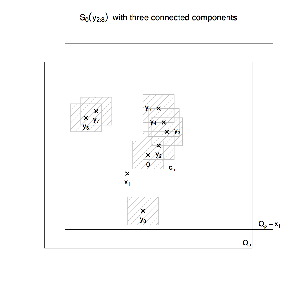
where, for any y2:k𝐑d(k1)subscript𝑦:2𝑘superscript𝐑𝑑𝑘1y_{2:k}\in\mathbf{R}^{d(k-1)}, the set S0(y2:k)𝐑dsubscript𝑆0subscript𝑦:2𝑘superscript𝐑𝑑S_{0}(y_{2:k})\subset\mathbf{R}^{d} is defined as (see Figure 1)

S0(y2:k):=𝔠ρj=2k(yj+𝔠ρ).assignsubscript𝑆0subscript𝑦:2𝑘subscript𝔠𝜌superscriptsubscript𝑗2𝑘subscript𝑦𝑗subscript𝔠𝜌S_{0}(y_{2:k}):=\mathfrak{c}_{\rho}\cup\bigcup_{j=2}^{k}(y_{j}+\mathfrak{c}_{\rho}).
Refer to caption
Figure 1: A configuration of points y2:8subscript𝑦:28y_{2:8}, where S0(y2:k)subscript𝑆0subscript𝑦:2𝑘S_{0}(y_{2:k}) has three connected components

It results from the above that

k(#Φ𝔔ρη(τ)=k)λd(𝔔ρ)(#Φ𝔔ρη{0}(τ)=k,gη{0}(0)>vρ(τ))=1(k1)!m=1k𝔔ρPx1[m]dx1,𝑘#superscriptsubscriptΦsubscript𝔔𝜌𝜂𝜏𝑘subscript𝜆𝑑subscript𝔔𝜌formulae-sequence#superscriptsubscriptΦsubscript𝔔𝜌𝜂0𝜏𝑘superscript𝑔𝜂00subscript𝑣𝜌𝜏1𝑘1superscriptsubscript𝑚1𝑘subscriptsubscript𝔔𝜌subscript𝑃subscript𝑥1delimited-[]𝑚differential-dsubscript𝑥1k\mathbb{P}\left(\,\#\Phi_{\mathfrak{Q}_{\rho}}^{\eta}(\tau)=k\,\right)-\lambda_{d}(\mathfrak{Q}_{\rho})\cdot\mathbb{P}\left(\,\#\Phi_{\mathfrak{Q}_{\rho}}^{\eta\cup\{0\}}(\tau)=k,g^{\eta\cup\{0\}}(0)>v_{\rho}(\tau)\,\right)\\ =\frac{1}{(k-1)!}\sum_{m=1}^{k}\int_{\mathfrak{Q}_{\rho}}P_{x_{1}}[m]\mathrm{d}x_{1},

where, for any x1𝐑dsubscript𝑥1superscript𝐑𝑑x_{1}\in\mathbf{R}^{d}, we write

Px1[m]:=(𝔔ρx1)k1Empx1(y2:k)dy2:k𝔔ρk1Emp0(y2:k)dy2:k.assignsubscript𝑃subscript𝑥1delimited-[]𝑚subscriptsuperscriptsubscript𝔔𝜌subscript𝑥1𝑘1subscript𝐸𝑚subscript𝑝subscript𝑥1subscript𝑦:2𝑘differential-dsubscript𝑦:2𝑘subscriptsuperscriptsubscript𝔔𝜌𝑘1subscript𝐸𝑚subscript𝑝0subscript𝑦:2𝑘differential-dsubscript𝑦:2𝑘P_{x_{1}}[m]:=\int_{(\mathfrak{Q}_{\rho}-x_{1})^{k-1}\cap E_{m}}p_{x_{1}}(y_{2:k})\mathrm{d}y_{2:k}-\int_{\mathfrak{Q}_{\rho}^{k-1}\cap E_{m}}p_{0}(y_{2:k})\mathrm{d}y_{2:k}. (3.4)

It is enough to show that for each 1mk1𝑚𝑘1\leq m\leq k, we have 𝔔ρPx1[m]dx1=o(λd(𝔔ρ)ρ1)subscriptsubscript𝔔𝜌subscript𝑃subscript𝑥1delimited-[]𝑚differential-dsubscript𝑥1𝑜subscript𝜆𝑑subscript𝔔𝜌superscript𝜌1\int_{\mathfrak{Q}_{\rho}}P_{x_{1}}[m]\mathrm{d}x_{1}=o\left(\lambda_{d}(\mathfrak{Q}_{\rho})\rho^{-1}\right). To do it, we begin with m=1𝑚1m=1 which deals with the case where there is exactly one connected component of size k𝑘k in S0(y2:k)subscript𝑆0subscript𝑦:2𝑘S_{0}(y_{2:k}). Then we extend our proof for m2𝑚2m\geq 2 by dividing the set S0(y2:k)subscript𝑆0subscript𝑦:2𝑘S_{0}(y_{2:k}) into its connected components.

First case (S0(y2:k)subscript𝑆0subscript𝑦:2𝑘S_{0}(y_{2:k}) has one connected component)

Assume that m=1𝑚1m=1 and let x1𝐑dsubscript𝑥1superscript𝐑𝑑x_{1}\in\mathbf{R}^{d} be fixed. We trivially obtain that

Px1[1]subscript𝑃subscript𝑥1delimited-[]1\displaystyle P_{x_{1}}[1] =((𝔔ρx1)𝔔ρ)k1E1(px1(y2:k)p0(y2:k))dy2:kabsentsubscriptsuperscriptsubscript𝔔𝜌subscript𝑥1subscript𝔔𝜌𝑘1subscript𝐸1subscript𝑝subscript𝑥1subscript𝑦:2𝑘subscript𝑝0subscript𝑦:2𝑘differential-dsubscript𝑦:2𝑘\displaystyle=\int_{\left((\mathfrak{Q}_{\rho}-x_{1})\cap\mathfrak{Q}_{\rho}\right)^{k-1}\cap E_{1}}\left(p_{x_{1}}(y_{2:k})-p_{0}(y_{2:k})\right)\mathrm{d}y_{2:k}
+(𝔔ρx1)k1E1px1(y2:k)𝕀jk:yj𝔔ρcdy2:ksubscriptsuperscriptsubscript𝔔𝜌subscript𝑥1𝑘1subscript𝐸1subscript𝑝subscript𝑥1subscript𝑦:2𝑘subscript𝕀:𝑗𝑘subscript𝑦𝑗superscriptsubscript𝔔𝜌𝑐differential-dsubscript𝑦:2𝑘\displaystyle+\int_{(\mathfrak{Q}_{\rho}-x_{1})^{k-1}\cap E_{1}}p_{x_{1}}(y_{2:k})\mathbb{I}_{\exists j\leq k:y_{j}\in\mathfrak{Q}_{\rho}^{c}}\,\mathrm{d}y_{2:k} (3.5)
𝔔ρk1E1p0(y2:k)𝕀jk:yj(𝔔ρx1)cdy2:k.subscriptsuperscriptsubscript𝔔𝜌𝑘1subscript𝐸1subscript𝑝0subscript𝑦:2𝑘subscript𝕀:𝑗𝑘subscript𝑦𝑗superscriptsubscript𝔔𝜌subscript𝑥1𝑐differential-dsubscript𝑦:2𝑘\displaystyle-\int_{\mathfrak{Q}_{\rho}^{k-1}\cap E_{1}}p_{0}(y_{2:k})\mathbb{I}_{\exists j\leq k:y_{j}\in(\mathfrak{Q}_{\rho}-x_{1})^{c}}\,\mathrm{d}y_{2:k}.

We provide below a suitable upper bound for each term considered in the right-hand side of the above equation.

Upper bound for the first term in (3.2)

Using the fact that for any events A,B,C𝐴𝐵𝐶A,B,C, we have |(AB)(AC)|(ABcC)+(ABCc)𝐴𝐵𝐴𝐶𝐴superscript𝐵𝑐𝐶𝐴𝐵superscript𝐶𝑐|\operatorname{\mathbb{P}}\left(\,A\cap B\,\right)-\operatorname{\mathbb{P}}\left(\,A\cap C\,\right)|\leq\operatorname{\mathbb{P}}\left(\,A\cap B^{c}\cap C\,\right)+\operatorname{\mathbb{P}}\left(\,A\cap B\cap C^{c}\,\right), we obtain

|((𝔔ρx1)𝔔ρ)k1E1(px1(y2:k)p0(y2:k))dy2:k|((𝔔ρx1)𝔔ρ)k1E1(gη{0,y2:k}(0,y2:k)>vρ(τ),M𝔔ρ(𝔔ρx1)η{0,y2:k}>vρ(τ))dy2:k+((𝔔ρx1)𝔔ρ)k1E1(gη{0,y2:k}(0,y2:k)>vρ(τ),M(𝔔ρx1)𝔔ρη{0,y2:k}>vρ(τ))dy2:k.subscriptsuperscriptsubscript𝔔𝜌subscript𝑥1subscript𝔔𝜌𝑘1subscript𝐸1subscript𝑝subscript𝑥1subscript𝑦:2𝑘subscript𝑝0subscript𝑦:2𝑘differential-dsubscript𝑦:2𝑘absentsubscriptsuperscriptsubscript𝔔𝜌subscript𝑥1subscript𝔔𝜌𝑘1subscript𝐸1formulae-sequencesuperscript𝑔𝜂0subscript𝑦:2𝑘0subscript𝑦:2𝑘subscript𝑣𝜌𝜏superscriptsubscript𝑀subscript𝔔𝜌subscript𝔔𝜌subscript𝑥1𝜂0subscript𝑦:2𝑘subscript𝑣𝜌𝜏differential-dsubscript𝑦:2𝑘subscriptsuperscriptsubscript𝔔𝜌subscript𝑥1subscript𝔔𝜌𝑘1subscript𝐸1formulae-sequencesuperscript𝑔𝜂0subscript𝑦:2𝑘0subscript𝑦:2𝑘subscript𝑣𝜌𝜏superscriptsubscript𝑀subscript𝔔𝜌subscript𝑥1subscript𝔔𝜌𝜂0subscript𝑦:2𝑘subscript𝑣𝜌𝜏differential-dsubscript𝑦:2𝑘\left|\int_{\left((\mathfrak{Q}_{\rho}-x_{1})\cap\mathfrak{Q}_{\rho}\right)^{k-1}\cap E_{1}}\left(p_{x_{1}}(y_{2:k})-p_{0}(y_{2:k})\right)\mathrm{d}y_{2:k}\right|\\ \begin{split}&\leq\int_{\left((\mathfrak{Q}_{\rho}-x_{1})\cap\mathfrak{Q}_{\rho}\right)^{k-1}\cap E_{1}}\mathbb{P}\left(\,g^{\eta\cup\{0,y_{2:k}\}}(0,y_{2:k})>v_{\rho}(\tau),M_{\mathfrak{Q}_{\rho}\setminus(\mathfrak{Q}_{\rho}-x_{1})}^{\eta\cup\{0,y_{2:k}\}}>v_{\rho}(\tau)\,\right)\mathrm{d}y_{2:k}\\ &+\int_{\left((\mathfrak{Q}_{\rho}-x_{1})\cap\mathfrak{Q}_{\rho}\right)^{k-1}\cap E_{1}}\mathbb{P}\left(\,g^{\eta\cup\{0,y_{2:k}\}}(0,y_{2:k})>v_{\rho}(\tau),M_{(\mathfrak{Q}_{\rho}-x_{1})\setminus\mathfrak{Q}_{\rho}}^{\eta\cup\{0,y_{2:k}\}}>v_{\rho}(\tau)\,\right)\mathrm{d}y_{2:k}.\end{split} (3.6)

To deal with the first term of the right-hand side of (3.6), we introduce the event:

E(x1):={y2:k𝐑(k1)d:S0(y2:k)(𝔔ρ(𝔔ρx1))=}.assignsuperscript𝐸subscript𝑥1conditional-setsubscript𝑦:2𝑘superscript𝐑𝑘1𝑑subscript𝑆0subscript𝑦:2𝑘subscript𝔔𝜌subscript𝔔𝜌subscript𝑥1E^{\varnothing}(x_{1}):=\left\{y_{2:k}\in\mathbf{R}^{(k-1)d}:S_{0}(y_{2:k})\cap\left(\mathfrak{Q}_{\rho}\setminus(\mathfrak{Q}_{\rho}-x_{1})\right)=\varnothing\right\}.

First, we assume that y2:kE(x1)E1subscript𝑦:2𝑘superscript𝐸subscript𝑥1subscript𝐸1y_{2:k}\in E^{\varnothing}(x_{1})\cap E_{1}. From (2.4), we know that {gη{0,y2:k}(0,y2:k)>vρ(τ)}Σ𝒜η{0,y2:k}superscript𝑔𝜂0subscript𝑦:2𝑘0subscript𝑦:2𝑘subscript𝑣𝜌𝜏superscriptsubscriptΣ𝒜𝜂0subscript𝑦:2𝑘\left\{g^{\eta\cup\{0,y_{2:k}\}}(0,y_{2:k})>v_{\rho}(\tau)\right\}\in\Sigma_{\mathcal{A}}^{\eta\cup\{0,y_{2:k}\}} and {M𝔔ρ(𝔔ρx1)η{0,y2:k}>vρ(τ)}Ση{0,y2:k}superscriptsubscript𝑀subscript𝔔𝜌subscript𝔔𝜌subscript𝑥1𝜂0subscript𝑦:2𝑘subscript𝑣𝜌𝜏superscriptsubscriptΣ𝜂0subscript𝑦:2𝑘\{M_{\mathfrak{Q}_{\rho}\setminus(\mathfrak{Q}_{\rho}-x_{1})}^{\eta\cup\{0,y_{2:k}\}}>v_{\rho}(\tau)\}\in\Sigma_{\mathcal{B}}^{\eta\cup\{0,y_{2:k}\}}, where

𝒜:={𝔦𝒱ρ:{0,y2:k}𝔦}and:={𝔧𝒱ρ:(𝔔ρ(𝔔ρx1))𝔧}.formulae-sequenceassign𝒜conditional-set𝔦subscript𝒱𝜌0subscript𝑦:2𝑘𝔦andassignconditional-set𝔧subscript𝒱𝜌subscript𝔔𝜌subscript𝔔𝜌subscript𝑥1𝔧\mathcal{A}:=\{\mathfrak{i}\in\mathcal{V}_{\rho}:\{0,y_{2:k}\}\cap\mathfrak{i}\neq\varnothing\}\quad\text{and}\quad\mathcal{B}:=\{\mathfrak{j}\in\mathcal{V}_{\rho}:(\mathfrak{Q}_{\rho}\setminus(\mathfrak{Q}_{\rho}-x_{1}))\cap\mathfrak{j}\neq\varnothing\}.

Since y2:kE(x1)subscript𝑦:2𝑘superscript𝐸subscript𝑥1y_{2:k}\in E^{\varnothing}(x_{1}), we have d(𝒜,)>D𝑑𝒜𝐷d(\mathcal{A},\mathcal{B})>D. It follows from Lemma 1, (i) that, conditional on 𝒜ρsubscript𝒜𝜌\mathscr{A}_{\rho}, the events {gη{0,y2:k}(0,y2:k)>vρ(τ)}superscript𝑔𝜂0subscript𝑦:2𝑘0subscript𝑦:2𝑘subscript𝑣𝜌𝜏\left\{g^{\eta\cup\{0,y_{2:k}\}}(0,y_{2:k})>v_{\rho}(\tau)\right\} and {M𝔔ρ(𝔔ρx1)η{0,y2:k}>vρ(τ)}superscriptsubscript𝑀subscript𝔔𝜌subscript𝔔𝜌subscript𝑥1𝜂0subscript𝑦:2𝑘subscript𝑣𝜌𝜏\left\{M_{\mathfrak{Q}_{\rho}\setminus(\mathfrak{Q}_{\rho}-x_{1})}^{\eta\cup\{0,y_{2:k}\}}>v_{\rho}(\tau)\right\} are independent. This implies that

(gη{0,y2:k}(0,y2:k)>vρ(τ),M𝔔ρ(𝔔ρx1)η{0,y2:k}>vρ(τ))𝕀y2:kE(x1)(𝒜ρ)1(gη{0,y2:k}(0,y2:k)>vρ(τ))(M𝔔ρ(𝔔ρx1)η{0,y2:k}>vρ(τ))+((𝒜ρ)c),\mathbb{P}\left(\,g^{\eta\cup\{0,y_{2:k}\}}(0,y_{2:k})>v_{\rho}(\tau),M_{\mathfrak{Q}_{\rho}\setminus(\mathfrak{Q}_{\rho}-x_{1})}^{\eta\cup\{0,y_{2:k}\}}>v_{\rho}(\tau)\,\right)\mathbb{I}_{y_{2:k}\in E^{\varnothing}(x_{1})}\,\\ \leq\operatorname{\mathbb{P}}\left(\,\mathscr{A}_{\rho}\,\right)^{-1}\cdot\mathbb{P}\left(\,g^{\eta\cup\{0,y_{2:k}\}}(0,y_{2:k})>v_{\rho}(\tau)\,\right)\cdot\mathbb{P}\left(\,M_{\mathfrak{Q}_{\rho}\setminus(\mathfrak{Q}_{\rho}-x_{1})}^{\eta\cup\{0,y_{2:k}\}}>v_{\rho}(\tau)\,\right)+\mathbb{P}\left(\,(\mathscr{A}_{\rho})^{c}\,\right),

where we have bounded the indicator function 𝕀y2:kE(x1)subscript𝕀subscript𝑦:2𝑘superscript𝐸subscript𝑥1\mathbb{I}_{y_{2:k}\in E^{\varnothing}(x_{1})} by 1. According to Lemma 1, (ii), we know that (𝒜ρ)1cραsubscript𝒜𝜌1𝑐superscript𝜌𝛼\operatorname{\mathbb{P}}\left(\,\mathscr{A}_{\rho}\,\right)\geq 1-c\cdot\rho^{-\alpha} for any α>0𝛼0\alpha>0. Moreover, since g𝑔g satisfies Condition (C), we have (gη{0,y2:k}(0,y2:k)>vρ(τ))cρ1superscript𝑔𝜂0subscript𝑦:2𝑘0subscript𝑦:2𝑘subscript𝑣𝜌𝜏𝑐superscript𝜌1\mathbb{P}\left(\,g^{\eta\cup\{0,y_{2:k}\}}(0,y_{2:k})>v_{\rho}(\tau)\,\right)\leq c\cdot\rho^{-1}. Besides, it results from the Slivnyak-Mecke formula that

(M𝔔ρ(𝔔ρx1)η{0,y2:k}>vρ(τ))=(z(𝔔ρ(𝔔ρx1))(η{0,y2:k}):gη{0,y2:k}(z)>vρ(τ))𝔼[zη𝔔ρ𝕀gη{0,y2:k}(z)>vρ(τ)]+j=2k(gη{0,y2:k}(yj)>vρ(τ))=𝔔ρ(gη{0,y2:k,z}(z)>vρ(τ))dz+j=2k(gη{0,y2:k}(yj)>vρ(τ))cλd(𝔔ρ)ρ1,superscriptsubscript𝑀subscript𝔔𝜌subscript𝔔𝜌subscript𝑥1𝜂0subscript𝑦:2𝑘subscript𝑣𝜌𝜏absent:𝑧subscript𝔔𝜌subscript𝔔𝜌subscript𝑥1𝜂0subscript𝑦:2𝑘superscript𝑔𝜂0subscript𝑦:2𝑘𝑧subscript𝑣𝜌𝜏𝔼delimited-[]subscript𝑧𝜂subscript𝔔𝜌subscript𝕀superscript𝑔𝜂0subscript𝑦:2𝑘𝑧subscript𝑣𝜌𝜏superscriptsubscript𝑗2𝑘superscript𝑔𝜂0subscript𝑦:2𝑘subscript𝑦𝑗subscript𝑣𝜌𝜏subscriptsubscript𝔔𝜌superscript𝑔𝜂0subscript𝑦:2𝑘𝑧𝑧subscript𝑣𝜌𝜏differential-d𝑧superscriptsubscript𝑗2𝑘superscript𝑔𝜂0subscript𝑦:2𝑘subscript𝑦𝑗subscript𝑣𝜌𝜏𝑐subscript𝜆𝑑subscript𝔔𝜌superscript𝜌1\mathbb{P}\left(\,M_{\mathfrak{Q}_{\rho}\setminus(\mathfrak{Q}_{\rho}-x_{1})}^{\eta\cup\{0,y_{2:k}\}}>v_{\rho}(\tau)\,\right)\\ \begin{split}&=\operatorname{\mathbb{P}}\left(\,\exists z\in(\mathfrak{Q}_{\rho}\setminus(\mathfrak{Q}_{\rho}-x_{1}))\cap(\eta\cup\{0,y_{2:k}\}):g^{\eta\cup\{0,y_{2:k}\}}(z)>v_{\rho}(\tau)\,\right)\\ &\leq\mathbb{E}\left[\,\sum_{z\in\eta\cap\mathfrak{Q}_{\rho}}\mathbb{I}_{g^{\eta\cup\{0,y_{2:k}\}}(z)>v_{\rho}(\tau)}\,\,\right]+\sum_{j=2}^{k}\mathbb{P}\left(\,g^{\eta\cup\{0,y_{2:k}\}}(y_{j})>v_{\rho}(\tau)\,\right)\\ &=\int_{\mathfrak{Q}_{\rho}}\mathbb{P}\left(\,g^{\eta\cup\{0,y_{2:k},z\}}(z)>v_{\rho}(\tau)\,\right)\mathrm{d}z+\sum_{j=2}^{k}\mathbb{P}\left(\,g^{\eta\cup\{0,y_{2:k}\}}(y_{j})>v_{\rho}(\tau)\,\right)\\ &\leq c\cdot\lambda_{d}(\mathfrak{Q}_{\rho})\rho^{-1},\end{split}

where the last line is also a consequence of Condition (C). This implies that

(gη{0,y2:k}(0,y2:k)>vρ(τ),M𝔔ρ(𝔔ρx1)η{0,y2:k}>vρ(τ))𝕀y2:kE(x1)E1cλd(𝔔ρ)ρ2.formulae-sequencesuperscript𝑔𝜂0subscript𝑦:2𝑘0subscript𝑦:2𝑘subscript𝑣𝜌𝜏superscriptsubscript𝑀subscript𝔔𝜌subscript𝔔𝜌subscript𝑥1𝜂0subscript𝑦:2𝑘subscript𝑣𝜌𝜏subscript𝕀subscript𝑦:2𝑘superscript𝐸subscript𝑥1subscript𝐸1𝑐subscript𝜆𝑑subscript𝔔𝜌superscript𝜌2\mathbb{P}\left(\,g^{\eta\cup\{0,y_{2:k}\}}(0,y_{2:k})>v_{\rho}(\tau),M_{\mathfrak{Q}_{\rho}\setminus(\mathfrak{Q}_{\rho}-x_{1})}^{\eta\cup\{0,y_{2:k}\}}>v_{\rho}(\tau)\,\right)\mathbb{I}_{y_{2:k}\in E^{\varnothing}(x_{1})\cap E_{1}}\,\leq c\cdot\lambda_{d}(\mathfrak{Q}_{\rho})\rho^{-2}. (3.7)

Secondly, we assume that y2:k(E(x1))cE1subscript𝑦:2𝑘superscriptsuperscript𝐸subscript𝑥1𝑐subscript𝐸1y_{2:k}\in(E^{\varnothing}(x_{1}))^{c}\cap E_{1}. In particular, we have

δ(0,𝔔ρ(𝔔ρx1))diam(S0(y2:k))cλd(𝔠ρ)1/d.𝛿0subscript𝔔𝜌subscript𝔔𝜌subscript𝑥1diamsubscript𝑆0subscript𝑦:2𝑘𝑐subscript𝜆𝑑superscriptsubscript𝔠𝜌1𝑑\delta(0,\mathfrak{Q}_{\rho}\setminus(\mathfrak{Q}_{\rho}-x_{1}))\leq\text{diam}(S_{0}(y_{2:k}))\leq c\cdot\lambda_{d}(\mathfrak{c}_{\rho})^{1/d}.

Since g𝑔g satisfies Condition (C), this implies that

(gη{0,y2:k}(0,y2:k)>vρ(τ),M𝔔ρ(𝔔ρx1)η{0,y2:k}>vρ(τ))𝕀y2:k(E(x1))cE1cρ1𝕀δ(0,𝔔ρ(𝔔ρx1))cλd(𝔠ρ)1/d.formulae-sequencesuperscript𝑔𝜂0subscript𝑦:2𝑘0subscript𝑦:2𝑘subscript𝑣𝜌𝜏superscriptsubscript𝑀subscript𝔔𝜌subscript𝔔𝜌subscript𝑥1𝜂0subscript𝑦:2𝑘subscript𝑣𝜌𝜏subscript𝕀subscript𝑦:2𝑘superscriptsuperscript𝐸subscript𝑥1𝑐subscript𝐸1𝑐superscript𝜌1subscript𝕀𝛿0subscript𝔔𝜌subscript𝔔𝜌subscript𝑥1𝑐subscript𝜆𝑑superscriptsubscript𝔠𝜌1𝑑\mathbb{P}\left(\,g^{\eta\cup\{0,y_{2:k}\}}(0,y_{2:k})>v_{\rho}(\tau),M_{\mathfrak{Q}_{\rho}\setminus(\mathfrak{Q}_{\rho}-x_{1})}^{\eta\cup\{0,y_{2:k}\}}>v_{\rho}(\tau)\,\right)\mathbb{I}_{y_{2:k}\in(E^{\varnothing}(x_{1}))^{c}\cap E_{1}}\,\\ \leq c\cdot\rho^{-1}\mathbb{I}_{\delta(0,\mathfrak{Q}_{\rho}\setminus(\mathfrak{Q}_{\rho}-x_{1}))\leq c\cdot\lambda_{d}(\mathfrak{c}_{\rho})^{1/d}}\,. (3.8)

Integrating over y2:k((𝔔ρx1)𝔔ρ)k1E1subscript𝑦:2𝑘superscriptsubscript𝔔𝜌subscript𝑥1subscript𝔔𝜌𝑘1subscript𝐸1y_{2:k}\in\left((\mathfrak{Q}_{\rho}-x_{1})\cap\mathfrak{Q}_{\rho}\right)^{k-1}\cap E_{1}, it follows from (3.7) and (3.8) that

((𝔔ρx1)𝔔ρ)k1E1(gη{0,y2:k}(0,y2:k)>vρ(τ),M𝔔ρ(𝔔ρx1)η{0,y2:k}>vρ(τ))dy2:kcλ(k1)d(E1)(λd(𝔔ρ)ρ2+ρ1𝕀δ(0,𝔔ρ(𝔔ρx1))cλd(𝔠ρ)1/d)cλd(𝔠ρ)k1(λd(𝔔ρ)ρ2+ρ1𝕀δ(0,𝔔ρ(𝔔ρx1))cλd(𝔠ρ)1/d),subscriptsuperscriptsubscript𝔔𝜌subscript𝑥1subscript𝔔𝜌𝑘1subscript𝐸1formulae-sequencesuperscript𝑔𝜂0subscript𝑦:2𝑘0subscript𝑦:2𝑘subscript𝑣𝜌𝜏superscriptsubscript𝑀subscript𝔔𝜌subscript𝔔𝜌subscript𝑥1𝜂0subscript𝑦:2𝑘subscript𝑣𝜌𝜏differential-dsubscript𝑦:2𝑘absent𝑐subscript𝜆𝑘1𝑑subscript𝐸1subscript𝜆𝑑subscript𝔔𝜌superscript𝜌2superscript𝜌1subscript𝕀𝛿0subscript𝔔𝜌subscript𝔔𝜌subscript𝑥1𝑐subscript𝜆𝑑superscriptsubscript𝔠𝜌1𝑑𝑐subscript𝜆𝑑superscriptsubscript𝔠𝜌𝑘1subscript𝜆𝑑subscript𝔔𝜌superscript𝜌2superscript𝜌1subscript𝕀𝛿0subscript𝔔𝜌subscript𝔔𝜌subscript𝑥1𝑐subscript𝜆𝑑superscriptsubscript𝔠𝜌1𝑑\int_{\left((\mathfrak{Q}_{\rho}-x_{1})\cap\mathfrak{Q}_{\rho}\right)^{k-1}\cap E_{1}}\mathbb{P}\left(\,g^{\eta\cup\{0,y_{2:k}\}}(0,y_{2:k})>v_{\rho}(\tau),M_{\mathfrak{Q}_{\rho}\setminus(\mathfrak{Q}_{\rho}-x_{1})}^{\eta\cup\{0,y_{2:k}\}}>v_{\rho}(\tau)\,\right)\mathrm{d}y_{2:k}\\ \begin{split}&\leq c\cdot\lambda_{(k-1)d}\left(E_{1}\right)\cdot\left(\lambda_{d}(\mathfrak{Q}_{\rho})\rho^{-2}+\rho^{-1}\mathbb{I}_{\delta(0,\mathfrak{Q}_{\rho}\setminus(\mathfrak{Q}_{\rho}-x_{1}))\leq c\cdot\lambda_{d}(\mathfrak{c}_{\rho})^{1/d}}\,\right)\\ &\leq c\cdot\lambda_{d}(\mathfrak{c}_{\rho})^{k-1}\cdot\left(\lambda_{d}(\mathfrak{Q}_{\rho})\cdot\rho^{-2}+\rho^{-1}\mathbb{I}_{\delta(0,\mathfrak{Q}_{\rho}\setminus(\mathfrak{Q}_{\rho}-x_{1}))\leq c\cdot\lambda_{d}(\mathfrak{c}_{\rho})^{1/d}}\,\,\right),\end{split} (3.9)

where the last line comes from the fact that λ(k1)d(E1)cλd(𝔠ρ)k1subscript𝜆𝑘1𝑑subscript𝐸1𝑐subscript𝜆𝑑superscriptsubscript𝔠𝜌𝑘1\lambda_{(k-1)d}(E_{1})\leq c\cdot\lambda_{d}(\mathfrak{c}_{\rho})^{k-1}.

Proceeding exactly along the same lines as above, by considering here the event:

F(x1):={y2:k𝐑(k1)d:S0(y2:k)((𝔔ρx1)𝔔ρ)=},assignsuperscript𝐹subscript𝑥1conditional-setsubscript𝑦:2𝑘superscript𝐑𝑘1𝑑subscript𝑆0subscript𝑦:2𝑘subscript𝔔𝜌subscript𝑥1subscript𝔔𝜌F^{\varnothing}(x_{1}):=\left\{y_{2:k}\in\mathbf{R}^{(k-1)d}:S_{0}(y_{2:k})\cap\left((\mathfrak{Q}_{\rho}-x_{1})\setminus\mathfrak{Q}_{\rho}\right)=\varnothing\right\},

we can show that the second term of the right-hand side of (3.6) can be bounded in a similar way, i.e.

((𝔔ρx1)𝔔ρ)k1E1(gη{0,y2:k}(0,y2:k)>vρ(τ),M(𝔔ρx1)𝔔ρη{0,y2:k}>vρ(τ))dy2:kcλd(𝔠ρ)k1(λd(𝔔ρ)ρ2+ρ1𝕀δ(0,(𝔔ρx1)𝔔ρ))cλd(𝔠ρ)1/d).\int_{\left((\mathfrak{Q}_{\rho}-x_{1})\cap\mathfrak{Q}_{\rho}\right)^{k-1}\cap E_{1}}\mathbb{P}\left(\,g^{\eta\cup\{0,y_{2:k}\}}(0,y_{2:k})>v_{\rho}(\tau),M_{(\mathfrak{Q}_{\rho}-x_{1})\setminus\mathfrak{Q}_{\rho}}^{\eta\cup\{0,y_{2:k}\}}>v_{\rho}(\tau)\,\right)\mathrm{d}y_{2:k}\\ \leq c\cdot\lambda_{d}(\mathfrak{c}_{\rho})^{k-1}\cdot\left(\lambda_{d}(\mathfrak{Q}_{\rho})\cdot\rho^{-2}+\rho^{-1}\mathbb{I}_{\delta(0,(\mathfrak{Q}_{\rho}-x_{1})\setminus\mathfrak{Q}_{\rho}))\leq c\cdot\lambda_{d}(\mathfrak{c}_{\rho})^{1/d}}\,\,\right).

This together with (3.6) and (3.9) implies that

((𝔔ρx1)𝔔ρ)k1E1(px1(y2:k)p0(y2:k))dy2:kcλd(𝔠ρ)k1λd(𝔔ρ)ρ2+cλd(𝔠ρ)k1ρ1(𝕀δ(0,𝔔ρ(𝔔ρx1))cλd(𝔠ρ)1/d+𝕀δ(0,(𝔔ρx1)𝔔ρ))cλd(𝔠ρ)1/d).\int_{\left((\mathfrak{Q}_{\rho}-x_{1})\cap\mathfrak{Q}_{\rho}\right)^{k-1}\cap E_{1}}\left(p_{x_{1}}(y_{2:k})-p_{0}(y_{2:k})\right)\mathrm{d}y_{2:k}\leq c\cdot\lambda_{d}(\mathfrak{c}_{\rho})^{k-1}\cdot\lambda_{d}(\mathfrak{Q}_{\rho})\cdot\rho^{-2}\\ +c\cdot\lambda_{d}(\mathfrak{c}_{\rho})^{k-1}\cdot\rho^{-1}\cdot\left(\mathbb{I}_{\delta(0,\mathfrak{Q}_{\rho}\setminus(\mathfrak{Q}_{\rho}-x_{1}))\leq c\cdot\lambda_{d}(\mathfrak{c}_{\rho})^{1/d}}\,+\mathbb{I}_{\delta(0,(\mathfrak{Q}_{\rho}-x_{1})\setminus\mathfrak{Q}_{\rho}))\leq c\cdot\lambda_{d}(\mathfrak{c}_{\rho})^{1/d}}\,\right).

This deals with the first term of the right-hand side in (3.2).

Upper bound for the second term in (3.2)

Trivially, this term equals 0: this comes from the fact that for ρ𝜌\rho large enough, we have

E1{y2:k𝐑(k1)d:jk s.t. yj𝔔ρc}=subscript𝐸1conditional-setsubscript𝑦:2𝑘superscript𝐑𝑘1𝑑𝑗𝑘 s.t. subscript𝑦𝑗superscriptsubscript𝔔𝜌𝑐E_{1}\cap\{y_{2:k}\in\mathbf{R}^{(k-1)d}:\exists j\leq k\text{ s.t. }y_{j}\in\mathfrak{Q}_{\rho}^{c}\}=\varnothing

since λd(𝔠ρ)=o(λd(𝔔ρ))subscript𝜆𝑑subscript𝔠𝜌𝑜subscript𝜆𝑑subscript𝔔𝜌\lambda_{d}(\mathfrak{c}_{\rho})=o\left(\lambda_{d}(\mathfrak{Q}_{\rho})\right).

Upper bound for the third term in (3.2)

To deal with this term, we notice that if E1{y2:k𝔔ρk1:jk s.t. yj(𝔔ρx1)c}subscript𝐸1conditional-setsubscript𝑦:2𝑘superscriptsubscript𝔔𝜌𝑘1𝑗𝑘 s.t. subscript𝑦𝑗superscriptsubscript𝔔𝜌subscript𝑥1𝑐E_{1}\cap\left\{y_{2:k}\in\mathfrak{Q}_{\rho}^{k-1}:\exists j\leq k\text{ s.t. }y_{j}\in(\mathfrak{Q}_{\rho}-x_{1})^{c}\right\}\neq\varnothing, then δ(0,𝔔ρ(𝔔ρx1))cλd(𝔠ρ)1/d𝛿0subscript𝔔𝜌subscript𝔔𝜌subscript𝑥1𝑐subscript𝜆𝑑superscriptsubscript𝔠𝜌1𝑑\delta\left(0,\mathfrak{Q}_{\rho}\setminus(\mathfrak{Q}_{\rho}-x_{1})\right)\leq c\cdot\lambda_{d}(\mathfrak{c}_{\rho})^{1/d} because diam(S0(y2:k))cλd(𝔠ρ)1/ddiamsubscript𝑆0subscript𝑦:2𝑘𝑐subscript𝜆𝑑superscriptsubscript𝔠𝜌1𝑑\text{diam}(S_{0}(y_{2:k}))\leq c\cdot\lambda_{d}(\mathfrak{c}_{\rho})^{1/d}. Besides, since p0(y2:k)cρ1subscript𝑝0subscript𝑦:2𝑘𝑐superscript𝜌1p_{0}(y_{2:k})\leq c\cdot\rho^{-1} according to Condition (C), we obtain by integrating over y2:k𝔔ρk1E1subscript𝑦:2𝑘superscriptsubscript𝔔𝜌𝑘1subscript𝐸1y_{2:k}\in\mathfrak{Q}_{\rho}^{k-1}\cap E_{1} that

𝔔ρk1E1p0(y2:k)𝕀jk:yj(𝔔ρx1)cdy2:kcλd(𝔠ρ)k1ρ1𝕀δ(0,𝔔ρ(𝔔ρx1))cλd(𝔠ρ)1/d.subscriptsuperscriptsubscript𝔔𝜌𝑘1subscript𝐸1subscript𝑝0subscript𝑦:2𝑘subscript𝕀:𝑗𝑘subscript𝑦𝑗superscriptsubscript𝔔𝜌subscript𝑥1𝑐differential-dsubscript𝑦:2𝑘𝑐subscript𝜆𝑑superscriptsubscript𝔠𝜌𝑘1superscript𝜌1subscript𝕀𝛿0subscript𝔔𝜌subscript𝔔𝜌subscript𝑥1𝑐subscript𝜆𝑑superscriptsubscript𝔠𝜌1𝑑\int_{\mathfrak{Q}_{\rho}^{k-1}\cap E_{1}}p_{0}(y_{2:k})\mathbb{I}_{\exists j\leq k:y_{j}\in(\mathfrak{Q}_{\rho}-x_{1})^{c}}\,\mathrm{d}y_{2:k}\leq c\cdot\lambda_{d}(\mathfrak{c}_{\rho})^{k-1}\cdot\rho^{-1}\cdot\mathbb{I}_{\delta\left(0,\mathfrak{Q}_{\rho}\setminus(\mathfrak{Q}_{\rho}-x_{1})\right)\leq c\cdot\lambda_{d}(\mathfrak{c}_{\rho})^{1/d}}\,.

This deals with the third term of the right-hand side in (3.2).

By considering the three upper bounds discussed above and by integrating over x1𝔔ρsubscript𝑥1subscript𝔔𝜌x_{1}\in\mathfrak{Q}_{\rho}, we get

|𝔔ρPx1[1]dx1|cλd(𝔠ρ)k1λd(𝔔ρ)2ρ2+cλd(𝔠ρ)k1ρ1λd({x1𝔔ρ:δ(0,𝔔ρ(𝔔ρx1)cλd(𝔠ρ)1/d})+cλd(𝔠ρ)k1ρ1λd({x1𝔔ρ:δ(0,(𝔔ρx1)𝔔ρcλd(𝔠ρ)1/d}).\left|\int_{\mathfrak{Q}_{\rho}}P_{x_{1}}[1]\mathrm{d}x_{1}\right|\leq c\cdot\lambda_{d}(\mathfrak{c}_{\rho})^{k-1}\cdot\lambda_{d}(\mathfrak{Q}_{\rho})^{2}\cdot\rho^{-2}\\ \begin{split}&+c\cdot\lambda_{d}(\mathfrak{c}_{\rho})^{k-1}\cdot\rho^{-1}\cdot\lambda_{d}\left(\left\{x_{1}\in\mathfrak{Q}_{\rho}:\delta(0,\mathfrak{Q}_{\rho}\setminus(\mathfrak{Q}_{\rho}-x_{1})\leq c\cdot\lambda_{d}(\mathfrak{c}_{\rho})^{1/d}\right\}\right)\\ &+c\cdot\lambda_{d}(\mathfrak{c}_{\rho})^{k-1}\cdot\rho^{-1}\cdot\lambda_{d}\left(\left\{x_{1}\in\mathfrak{Q}_{\rho}:\delta(0,(\mathfrak{Q}_{\rho}-x_{1})\setminus\mathfrak{Q}_{\rho}\leq c\cdot\lambda_{d}(\mathfrak{c}_{\rho})^{1/d}\right\}\right).\end{split}

We can easily prove that if x1𝔔ρsubscript𝑥1subscript𝔔𝜌x_{1}\in\mathfrak{Q}_{\rho} is such that δ(0,𝔔ρ(𝔔ρx1)cλd(𝔠ρ)1/d\delta(0,\mathfrak{Q}_{\rho}\setminus(\mathfrak{Q}_{\rho}-x_{1})\leq c\cdot\lambda_{d}(\mathfrak{c}_{\rho})^{1/d}, then x1𝔔ρ(𝔔ρc1/d𝔠ρ)subscript𝑥1subscript𝔔𝜌symmetric-differencesubscript𝔔𝜌superscript𝑐1𝑑subscript𝔠𝜌x_{1}\in\mathfrak{Q}_{\rho}\setminus(\mathfrak{Q}_{\rho}\ominus c^{1/d}\cdot\mathfrak{c}_{\rho}). Hence

λd({x1𝔔ρ:δ(0,𝔔ρ(𝔔ρx1)cλd(𝔠ρ)1/d})λd(𝔔ρ(𝔔ρc1/d𝔠ρ))=O(λd(𝔔ρ)(d1)/dλd(𝔠ρ)1/d).\begin{split}\lambda_{d}\left(\left\{x_{1}\in\mathfrak{Q}_{\rho}:\delta(0,\mathfrak{Q}_{\rho}\setminus(\mathfrak{Q}_{\rho}-x_{1})\leq c\cdot\lambda_{d}(\mathfrak{c}_{\rho})^{1/d}\right\}\right)&\leq\lambda_{d}\left(\mathfrak{Q}_{\rho}\setminus(\mathfrak{Q}_{\rho}\ominus c^{1/d}\cdot\mathfrak{c}_{\rho})\right)\\ &=O\left(\lambda_{d}(\mathfrak{Q}_{\rho})^{(d-1)/d}\cdot\lambda_{d}(\mathfrak{c}_{\rho})^{1/d}\right).\end{split}

Moreover, for ρ𝜌\rho large enough, we have

λd({x1𝔔ρ:δ(0,(𝔔ρx1)𝔔ρcλd(𝔠0)1/d})=0\lambda_{d}\left(\{x_{1}\in\mathfrak{Q}_{\rho}:\delta(0,(\mathfrak{Q}_{\rho}-x_{1})\setminus\mathfrak{Q}_{\rho}\leq c\cdot\lambda_{d}(\mathfrak{c}_{0})^{1/d}\}\right)=0

since λd(𝔠ρ)=o(λd(𝔔ρ))subscript𝜆𝑑subscript𝔠𝜌𝑜subscript𝜆𝑑subscript𝔔𝜌\lambda_{d}(\mathfrak{c}_{\rho})=o\left(\lambda_{d}(\mathfrak{Q}_{\rho})\right). From (2.1), we deduce that

|𝔔ρPx1[1]dx1|c(λd(𝔠ρ)k1+1/dλd(𝔔ρ)1/d)(λd(𝔔ρ)ρ1)=o(λd(𝔔ρ)ρ1).subscriptsubscript𝔔𝜌subscript𝑃subscript𝑥1delimited-[]1differential-dsubscript𝑥1𝑐subscript𝜆𝑑superscriptsubscript𝔠𝜌𝑘11𝑑subscript𝜆𝑑superscriptsubscript𝔔𝜌1𝑑subscript𝜆𝑑subscript𝔔𝜌superscript𝜌1𝑜subscript𝜆𝑑subscript𝔔𝜌superscript𝜌1\left|\int_{\mathfrak{Q}_{\rho}}P_{x_{1}}[1]\mathrm{d}x_{1}\right|\leq c\cdot\left(\lambda_{d}(\mathfrak{c}_{\rho})^{k-1+1/d}\cdot\lambda_{d}(\mathfrak{Q}_{\rho})^{-1/d}\right)\cdot\left(\lambda_{d}(\mathfrak{Q}_{\rho})\cdot\rho^{-1}\right)=o\left(\lambda_{d}(\mathfrak{Q}_{\rho})\cdot\rho^{-1}\right).

This concludes the proof for the case m=1𝑚1m=1.

Second case (S0(y2:k)subscript𝑆0subscript𝑦:2𝑘S_{0}(y_{2:k}) has m𝑚m connected component with m2𝑚2m\geq 2 )

Assume that m2𝑚2m\geq 2 and y2:kEmsubscript𝑦:2𝑘subscript𝐸𝑚y_{2:k}\in E_{m}.

First, we provide below a uniform upper bound for px(y2:k)subscript𝑝𝑥subscript𝑦:2𝑘p_{x}(y_{2:k}), with x𝔔ρ𝑥subscript𝔔𝜌x\in\mathfrak{Q}_{\rho}. Since y2:kEmsubscript𝑦:2𝑘subscript𝐸𝑚y_{2:k}\in E_{m}, we can divide S0(y2:k)subscript𝑆0subscript𝑦:2𝑘S_{0}(y_{2:k}) into its m𝑚m connected components, say C1(y2:k),,Cm(y2:k)subscript𝐶1subscript𝑦:2𝑘subscript𝐶𝑚subscript𝑦:2𝑘C_{1}(y_{2:k}),\ldots,C_{m}(y_{2:k}). For each 1lm1𝑙𝑚1\leq l\leq m, let Jl{1,,k}subscript𝐽𝑙1𝑘J_{l}\subset\{1,\ldots,k\} be the set of indices j𝑗j such that Cl(y2:k)=jJl(yj+𝔠ρ)subscript𝐶𝑙subscript𝑦:2𝑘subscript𝑗subscript𝐽𝑙subscript𝑦𝑗subscript𝔠𝜌C_{l}(y_{2:k})=\bigcup_{j\in J_{l}}(y_{j}+\mathfrak{c}_{\rho}), with y1:=0assignsubscript𝑦10y_{1}:=0. In particular, we have

px(y2:k)(gη{0,y2:k}(0,y2:k)>vρ(τ))=(l=1m{gη{0,y2:k}(yJl)>vρ(τ)}),subscript𝑝𝑥subscript𝑦:2𝑘superscript𝑔𝜂0subscript𝑦:2𝑘0subscript𝑦:2𝑘subscript𝑣𝜌𝜏superscriptsubscript𝑙1𝑚superscript𝑔𝜂0subscript𝑦:2𝑘subscript𝑦subscript𝐽𝑙subscript𝑣𝜌𝜏p_{x}(y_{2:k})\leq\operatorname{\mathbb{P}}\left(\,g^{\eta\cup\{0,y_{2:k}\}}(0,y_{2:k})>v_{\rho}(\tau)\,\right)=\mathbb{P}\left(\,\bigcap_{l=1}^{m}\left\{g^{\eta\cup\{0,y_{2:k}\}}(y_{J_{l}})>v_{\rho}(\tau)\right\}\,\right),

where we recall that gη{0,y2:k}(yJl)>vρ(τ)superscript𝑔𝜂0subscript𝑦:2𝑘subscript𝑦subscript𝐽𝑙subscript𝑣𝜌𝜏g^{\eta\cup\{0,y_{2:k}\}}(y_{J_{l}})>v_{\rho}(\tau) means that gη{0,y2:k}(y)>vρ(τ)superscript𝑔𝜂0subscript𝑦:2𝑘𝑦subscript𝑣𝜌𝜏g^{\eta\cup\{0,y_{2:k}\}}(y)>v_{\rho}(\tau) for any yJl𝑦subscript𝐽𝑙y\in J_{l}. In the same spirit as in the case where S0(y2:k)subscript𝑆0subscript𝑦:2𝑘S_{0}(y_{2:k}) has one connected component, we deduce from Lemma 1, (i) that, conditional on the event 𝒜ρsubscript𝒜𝜌\mathscr{A}_{\rho}, the events {gη{0,y2:k}(yJl)>vρ(τ)}superscript𝑔𝜂0subscript𝑦:2𝑘subscript𝑦subscript𝐽𝑙subscript𝑣𝜌𝜏\{g^{\eta\cup\{0,y_{2:k}\}}(y_{J_{l}})>v_{\rho}(\tau)\}, 1lm1𝑙𝑚1\leq l\leq m, are independent. This gives

px(y2:k)(𝒜ρ)(m1)l=1m(gη{0,y2:k}(yJl)>vρ(τ))+(𝒜ρc).p_{x}(y_{2:k})\leq\operatorname{\mathbb{P}}\left(\,\mathscr{A}_{\rho}\,\right)^{-(m-1)}\cdot\prod_{l=1}^{m}\mathbb{P}\left(\,g^{\eta\cup\{0,y_{2:k}\}}(y_{J_{l}})>v_{\rho}(\tau)\,\right)+\operatorname{\mathbb{P}}\left(\,\mathscr{A}_{\rho}^{c}\,\right).

Since g𝑔g satisfies Condition (C), it follows from Lemma 1, (ii) that there exists a constant c>0𝑐0c>0 such that, for any x𝔔ρ𝑥subscript𝔔𝜌x\in\mathfrak{Q}_{\rho} and for any y2:kEmsubscript𝑦:2𝑘subscript𝐸𝑚y_{2:k}\in E_{m}, we have px(y2:k)cρmsubscript𝑝𝑥subscript𝑦:2𝑘𝑐superscript𝜌𝑚p_{x}(y_{2:k})\leq c\cdot\rho^{-m}.

Now, we are able to provide an upper bound for |𝔔ρPx1[m]dx1|subscriptsubscript𝔔𝜌subscript𝑃subscript𝑥1delimited-[]𝑚differential-dsubscript𝑥1\left|\int_{\mathfrak{Q}_{\rho}}P_{x_{1}}[m]\mathrm{d}x_{1}\right|. Indeed, integrating over y2:ksubscript𝑦:2𝑘y_{2:k} in the right-hand side of (3.4), we have

|Px1[m]|cρmsupx𝔔ρλ(k1)d((𝔔ρx)k1Em)cρmλd(𝔔ρ)m1λd(𝔠ρ)km.subscript𝑃subscript𝑥1delimited-[]𝑚𝑐superscript𝜌𝑚subscriptsupremum𝑥subscript𝔔𝜌subscript𝜆𝑘1𝑑superscriptsubscript𝔔𝜌𝑥𝑘1subscript𝐸𝑚𝑐superscript𝜌𝑚subscript𝜆𝑑superscriptsubscript𝔔𝜌𝑚1subscript𝜆𝑑superscriptsubscript𝔠𝜌𝑘𝑚|P_{x_{1}}[m]|\leq c\cdot\rho^{-m}\cdot\sup_{x\in\mathfrak{Q}_{\rho}}\lambda_{(k-1)d}((\mathfrak{Q}_{\rho}-x)^{k-1}\cap E_{m})\leq c\cdot\rho^{-m}\cdot\lambda_{d}(\mathfrak{Q}_{\rho})^{m-1}\cdot\lambda_{d}(\mathfrak{c}_{\rho})^{k-m}.

Integrating over x1𝔔ρsubscript𝑥1subscript𝔔𝜌x_{1}\in\mathfrak{Q}_{\rho}, we get

|𝔔ρPx1[m]dx1|c(ρ1λd(𝔔ρ)λd(𝔠ρ)(km)/(m1))m1(λd(𝔔ρ)ρ1)=o(λd(𝔔ρ)ρ1).subscriptsubscript𝔔𝜌subscript𝑃subscript𝑥1delimited-[]𝑚differential-dsubscript𝑥1𝑐superscriptsuperscript𝜌1subscript𝜆𝑑subscript𝔔𝜌subscript𝜆𝑑superscriptsubscript𝔠𝜌𝑘𝑚𝑚1𝑚1subscript𝜆𝑑subscript𝔔𝜌superscript𝜌1𝑜subscript𝜆𝑑subscript𝔔𝜌superscript𝜌1\left|\int_{\mathfrak{Q}_{\rho}}P_{x_{1}}[m]\mathrm{d}x_{1}\right|\leq c\cdot\left(\rho^{-1}\cdot\lambda_{d}(\mathfrak{Q}_{\rho})\cdot\lambda_{d}(\mathfrak{c}_{\rho})^{(k-m)/(m-1)}\right)^{m-1}\cdot\left(\lambda_{d}(\mathfrak{Q}_{\rho})\cdot\rho^{-1}\right)=o\left(\lambda_{d}(\mathfrak{Q}_{\rho})\cdot\rho^{-1}\right).

This concludes the proof of Proposition 3 for any k2𝑘2k\geq 2. The case k=1𝑘1k=1 is much more simple than the case k2𝑘2k\geq 2 and can be dealt by following the same lines as above and by noting that

(#Φ𝔔ρη(τ)=1)λd(𝔔ρ)(#Φ𝔔ρη{0}(τ)=1,gη{0}(0)>vρ(τ))=𝔔ρ(px1p0)dx1,#superscriptsubscriptΦsubscript𝔔𝜌𝜂𝜏1subscript𝜆𝑑subscript𝔔𝜌formulae-sequence#superscriptsubscriptΦsubscript𝔔𝜌𝜂0𝜏1superscript𝑔𝜂00subscript𝑣𝜌𝜏subscriptsubscript𝔔𝜌subscript𝑝subscript𝑥1subscript𝑝0differential-dsubscript𝑥1\mathbb{P}\left(\,\#\Phi_{\mathfrak{Q}_{\rho}}^{\eta}(\tau)=1\,\right)-\lambda_{d}(\mathfrak{Q}_{\rho})\cdot\mathbb{P}\left(\,\#\Phi_{\mathfrak{Q}_{\rho}}^{\eta\cup\{0\}}(\tau)=1,g^{\eta\cup\{0\}}(0)>v_{\rho}(\tau)\,\right)=\int_{\mathfrak{Q}_{\rho}}(p_{x_{1}}-p_{0})\mathrm{d}x_{1},

where, for any x𝔔ρ𝑥subscript𝔔𝜌x\in\mathfrak{Q}_{\rho}, we write px:=(gη{0}(0)>vρ(τ),M(𝔔ρx){0}η{0}vρ(τ))assignsubscript𝑝𝑥formulae-sequencesuperscript𝑔𝜂00subscript𝑣𝜌𝜏subscriptsuperscript𝑀𝜂0subscript𝔔𝜌𝑥0subscript𝑣𝜌𝜏p_{x}:=\mathbb{P}\left(\,g^{\eta\cup\{0\}}(0)>v_{\rho}(\tau),M^{\eta\cup\{0\}}_{(\mathfrak{Q}_{\rho}-x)\setminus\{0\}}\leq v_{\rho}(\tau)\,\right). \square

3.3 Our main theorem

Let g𝑔g be a geometric characteristic such that (1.6) holds for some τ0>0subscript𝜏00\tau_{0}>0. According to Leadbetter [18], we say that the extremal index θ[0,1]𝜃01\theta\in[0,1] of the Poisson-Voronoi tessellation exists if limρ(#Φ𝐖ρη(τ0)=0)=eθτ0subscript𝜌#subscriptsuperscriptΦ𝜂subscript𝐖𝜌subscript𝜏00superscript𝑒𝜃subscript𝜏0\lim_{\rho\rightarrow\infty}\mathbb{P}(\#\Phi^{\eta}_{\mathbf{W}_{\rho}}(\tau_{0})=0)=e^{-\theta\tau_{0}}. We are now prepared to state our main theorem on the weak convergence of the point process Φ𝐖ρη(τ)subscriptsuperscriptΦ𝜂subscript𝐖𝜌𝜏\Phi^{\eta}_{\mathbf{W}_{\rho}}(\tau) for each τ>0𝜏0\tau>0.

Theorem 4.

Let g𝑔g be a geometric characteristic satisfying Condition (C). Assume that there exist τ0>0subscript𝜏00\tau_{0}>0 such that (1.6) holds and (ak)k1subscriptsubscript𝑎𝑘𝑘1(a_{k})_{k\geq 1} such that πk,𝔔ρ(τ0)aksubscript𝜋𝑘subscript𝔔𝜌subscript𝜏0subscript𝑎𝑘\pi_{k,\mathfrak{Q}_{\rho}}(\tau_{0})\leq a_{k} for any k1𝑘1k\geq 1 and any ρ>0𝜌0\rho>0, with k=1ak<superscriptsubscript𝑘1subscript𝑎𝑘\sum_{k=1}^{\infty}a_{k}<\infty.

  1. (i)

    The following assertions are equivalent:

    1. (A)

      there exists θ(0,1]𝜃01\theta\in(0,1] such that limρ(#Φ𝐖ρη(τ0)=0)=eθτ0subscript𝜌#subscriptsuperscriptΦ𝜂subscript𝐖𝜌subscript𝜏00superscript𝑒𝜃subscript𝜏0\lim_{\rho\rightarrow\infty}\mathbb{P}(\#\Phi^{\eta}_{\mathbf{W}_{\rho}}(\tau_{0})=0)=e^{-\theta\tau_{0}} and the following limit exist pk:=limρpk,𝔔ρ(τ0)assignsubscript𝑝𝑘subscript𝜌subscript𝑝𝑘subscript𝔔𝜌subscript𝜏0p_{k}:=\lim_{\rho\rightarrow\infty}p_{k,\mathfrak{Q}_{\rho}}(\tau_{0}) for any k1𝑘1k\geq 1;

    2. (B)

      for any τ>0𝜏0\tau>0, the point process Φ𝐖ρη(τ)subscriptsuperscriptΦ𝜂subscript𝐖𝜌𝜏\Phi^{\eta}_{\mathbf{W}_{\rho}}(\tau) converges to a homogeneous compound Poisson point process in W:=[1/2,1/2]dassign𝑊superscript1212𝑑W:=\left[-1/2,1/2\right]^{d} with intensity ν(τ)>0𝜈𝜏0\nu(\tau)>0 and cluster size distributions πk:=limρπk,𝔔ρ(τ0)assignsubscript𝜋𝑘subscript𝜌subscript𝜋𝑘subscript𝔔𝜌subscript𝜏0\pi_{k}:=\lim_{\rho\rightarrow\infty}\pi_{k,\mathfrak{Q}_{\rho}}(\tau_{0}), with k1𝑘1k\geq 1.

  2. (ii)

    If one of the above assertions holds, we have pk=kθπksubscript𝑝𝑘𝑘𝜃subscript𝜋𝑘p_{k}=k\theta\pi_{k} for any k1𝑘1k\geq 1 and θ=k=1k1pk𝜃superscriptsubscript𝑘1superscript𝑘1subscript𝑝𝑘\theta=\sum_{k=1}^{\infty}k^{-1}p_{k}.

Our theorem provides a new characterization of the extremal index. Indeed, this index was previously interpreted as the reciprocal of the mean of the cluster size distribution π𝜋\pi. Now, it can be viewed as the mean of the reciprocal of the Palm version of the cluster size. Besides, our new characterization: θ=k=1k1pk𝜃superscriptsubscript𝑘1superscript𝑘1subscript𝑝𝑘\theta=\sum_{k=1}^{\infty}k^{-1}p_{k} will be extensively used in Section 4 to estimate the extremal indices for various geometric characteristics.

To prove Theorem 4, we associate with the point process Φ𝐖ρη(τ)subscriptsuperscriptΦ𝜂subscript𝐖𝜌𝜏\Phi^{\eta}_{\mathbf{W}_{\rho}}(\tau) its Laplace transform 𝕃ρsubscript𝕃𝜌\mathbb{L}_{\rho} defined as follows: for any continuous function f:W𝐑+:𝑓𝑊subscript𝐑f:W\rightarrow\mathbf{R}_{+}, we have

𝕃ρ(f):=𝔼[exp(yΦ𝐖ρη(τ)f(y))]assignsubscript𝕃𝜌𝑓𝔼delimited-[]subscript𝑦subscriptsuperscriptΦ𝜂subscript𝐖𝜌𝜏𝑓𝑦\mathbb{L}_{\rho}(f):=\mathbb{E}\left[\,\exp\left(-\sum_{y\in\Phi^{\eta}_{\mathbf{W}_{\rho}}(\tau)}f(y)\right)\,\right].

It is well-known that the weak convergence of Φ𝐖ρη(τ)subscriptsuperscriptΦ𝜂subscript𝐖𝜌𝜏\Phi^{\eta}_{\mathbf{W}_{\rho}}(\tau) is equivalent to the convergence of its Laplace transform for any positive and continuous function f𝑓f. For a sequence of real random variables, the weak convergence of the point process of exceedances has been investigated in [15] and generalized to random fields on 𝐍+dsuperscriptsubscript𝐍𝑑\mathbf{N}_{+}^{d} in [12]. We use below the same type of approach. However, we have to take into account specific features of random tessellations in 𝐑dsuperscript𝐑𝑑\mathbf{R}^{d}.

The first step consists in showing that exceedances over disjoint sub-cubes behave asymptotically as if they were independent. To do it, we divide 𝐖ρsubscript𝐖𝜌\mathbf{W}_{\rho} into mρdsuperscriptsubscript𝑚𝜌𝑑m_{\rho}^{d} disjoint sub-cubes 𝔅[l]𝔅delimited-[]𝑙\mathfrak{B}[l], l=1,,mρd𝑙1superscriptsubscript𝑚𝜌𝑑l=1,\ldots,m_{\rho}^{d}, with the same volume as 𝔔ρsubscript𝔔𝜌\mathfrak{Q}_{\rho}, where mρsubscript𝑚𝜌m_{\rho} is defined in (2.2).

Lemma 5.
  1. (i)

    For any measurable function f:W𝐑+:𝑓𝑊subscript𝐑f:W\rightarrow\mathbf{R}_{+}, we have

    𝕃ρ(f)l=1mρd𝔼[exp(yΦ𝐖ρη(τ)ρ1/d𝔅[l]f(y))]ρ0.subscript𝕃𝜌𝑓superscriptsubscriptproduct𝑙1superscriptsubscript𝑚𝜌𝑑𝔼delimited-[]subscript𝑦subscriptsuperscriptΦ𝜂subscript𝐖𝜌𝜏superscript𝜌1𝑑𝔅delimited-[]𝑙𝑓𝑦𝜌0\mathbb{L}_{\rho}(f)-\prod_{l=1}^{m_{\rho}^{d}}\mathbb{E}\left[\,\exp\left(-\sum_{y\in\Phi^{\eta}_{\mathbf{W}_{\rho}}(\tau)\cap\rho^{-1/d}\mathfrak{B}[l]}f(y)\right)\,\right]\underset{\rho\rightarrow\infty}{\longrightarrow}0.
  2. (ii)

    Moreover, we have

    (M𝐖ρηvρ(τ))l=1mρd(M𝔅[l]ηvρ(τ))ρ0.superscriptsubscript𝑀subscript𝐖𝜌𝜂subscript𝑣𝜌𝜏superscriptsubscriptproduct𝑙1superscriptsubscript𝑚𝜌𝑑superscriptsubscript𝑀𝔅delimited-[]𝑙𝜂subscript𝑣𝜌𝜏𝜌0\mathbb{P}\left(M_{\mathbf{W}_{\rho}}^{\eta}\leq v_{\rho}(\tau)\right)-\prod_{l=1}^{m_{\rho}^{d}}\mathbb{P}\left(M_{\mathfrak{B}[l]}^{\eta}\,\leq v_{\rho}(\tau)\right)\underset{\rho\rightarrow\infty}{\longrightarrow}0.

Proof We begin with the first assertion. For any lmρd𝑙superscriptsubscript𝑚𝜌𝑑l\leq m_{\rho}^{d}, we write 𝔅[l]:=𝔅[l]𝔠ρassignsuperscript𝔅delimited-[]𝑙symmetric-difference𝔅delimited-[]𝑙subscript𝔠𝜌\mathfrak{B}^{\circ}[l]:=\mathfrak{B}[l]\ominus\mathfrak{c}_{\rho}. Let

Lρ,l(f)=exp(yΦ𝐖ρη(τ)ρ1/d𝔅[l]f(y))andLρ,l(f)=exp(yΦ𝐖ρη(τ)ρ1/d𝔅[l]f(y)).formulae-sequencesubscript𝐿𝜌𝑙𝑓subscript𝑦subscriptsuperscriptΦ𝜂subscript𝐖𝜌𝜏superscript𝜌1𝑑𝔅delimited-[]𝑙𝑓𝑦andsuperscriptsubscript𝐿𝜌𝑙𝑓subscript𝑦subscriptsuperscriptΦ𝜂subscript𝐖𝜌𝜏superscript𝜌1𝑑superscript𝔅delimited-[]𝑙𝑓𝑦L_{\rho,l}(f)\,=\exp\left(-\sum_{y\in\Phi^{\eta}_{\mathbf{W}_{\rho}}(\tau)\cap\rho^{-1/d}\mathfrak{B}[l]}f(y)\right)\quad\text{and}\quad L_{\rho,l}^{\circ}(f)=\exp\left(-\sum_{y\in\Phi^{\eta}_{\mathbf{W}_{\rho}}(\tau)\cap\rho^{-1/d}\mathfrak{B}^{\circ}[l]}f(y)\,\right).

We write

𝕃ρ(f)l=1mρd𝔼[Lρ,l(f)]=ΔLρ,1(f)+ΔLρ,2(f)+ΔLρ,3(f)+ΔLρ,4(f),subscript𝕃𝜌𝑓superscriptsubscriptproduct𝑙1superscriptsubscript𝑚𝜌𝑑𝔼delimited-[]subscript𝐿𝜌𝑙𝑓Δsubscript𝐿𝜌1𝑓Δsubscript𝐿𝜌2𝑓Δsubscript𝐿𝜌3𝑓Δsubscript𝐿𝜌4𝑓\mathbb{L}_{\rho}(f)-\prod_{l=1}^{m_{\rho}^{d}}\mathbb{E}\left[L_{\rho,l}(f)\right]=\Delta L_{\rho,1}(f)+\Delta L_{\rho,2}(f)+\Delta L_{\rho,3}(f)+\Delta L_{\rho,4}(f),

where

ΔLρ,1(f)=𝔼[l=1mρdLρ,l(f)]𝔼[l=1mρdLρ,l(f)],Δsubscript𝐿𝜌1𝑓𝔼delimited-[]superscriptsubscriptproduct𝑙1superscriptsubscript𝑚𝜌𝑑subscript𝐿𝜌𝑙𝑓𝔼delimited-[]superscriptsubscriptproduct𝑙1superscriptsubscript𝑚𝜌𝑑superscriptsubscript𝐿𝜌𝑙𝑓\Delta L_{\rho,1}(f)=\mathbb{E}\left[\prod_{l=1}^{m_{\rho}^{d}}L_{\rho,l}(f)\,\right]-\mathbb{E}\left[\prod_{l=1}^{m_{\rho}^{d}}L_{\rho,l}^{\circ}(f)\,\right],
ΔLρ,2(f)=𝔼[l=1mρdLρ,l(f)]l=1mρd𝔼[Lρ,l(f)],Δsubscript𝐿𝜌2𝑓𝔼delimited-[]superscriptsubscriptproduct𝑙1superscriptsubscript𝑚𝜌𝑑superscriptsubscript𝐿𝜌𝑙𝑓superscriptsubscriptproduct𝑙1superscriptsubscript𝑚𝜌𝑑𝔼delimited-[]superscriptsubscript𝐿𝜌𝑙𝑓\Delta L_{\rho,2}(f)=\mathbb{E}\left[\prod_{l=1}^{m_{\rho}^{d}}L_{\rho,l}^{\circ}(f)\,\right]-\prod_{l=1}^{m_{\rho}^{d}}\mathbb{E}\left[\,L_{\rho,l}^{\circ}(f)\,\right],
ΔLρ,3(f)=l=1mρd𝔼[Lρ,l(f)]l=1mρd𝔼[Lρ,l(f)],Δsubscript𝐿𝜌3𝑓superscriptsubscriptproduct𝑙1superscriptsubscript𝑚𝜌𝑑𝔼delimited-[]superscriptsubscript𝐿𝜌𝑙𝑓superscriptsubscriptproduct𝑙1superscriptsubscript𝑚𝜌𝑑𝔼delimited-[]subscript𝐿𝜌𝑙𝑓\Delta L_{\rho,3}(f)=\prod_{l=1}^{m_{\rho}^{d}}\mathbb{E}\left[\,L_{\rho,l}^{\circ}(f)\,\right]-\prod_{l=1}^{m_{\rho}^{d}}\mathbb{E}\left[L_{\rho,l}(f)\,\right],
ΔLρ,4(f)=𝔼[exp(yΦ𝐖ρη(τ)f(y))]𝔼[l=1mρdLρ,l(f)].Δsubscript𝐿𝜌4𝑓𝔼delimited-[]subscript𝑦subscriptsuperscriptΦ𝜂subscript𝐖𝜌𝜏𝑓𝑦𝔼delimited-[]superscriptsubscriptproduct𝑙1superscriptsubscript𝑚𝜌𝑑subscript𝐿𝜌𝑙𝑓\Delta L_{\rho,4}(f)=\mathbb{E}\left[\,\exp\left(-\sum_{y\in\Phi^{\eta}_{\mathbf{W}_{\rho}}(\tau)}f(y)\right)\,\right]-\mathbb{E}\left[\prod_{l=1}^{m_{\rho}^{d}}L_{\rho,l}(f)\,\right].

We prove below that each term converges to 00. For the third term, using the fact that |xiyi||xiyi|productsubscript𝑥𝑖productsubscript𝑦𝑖subscript𝑥𝑖subscript𝑦𝑖|\prod x_{i}-\prod y_{i}|\leq\sum|x_{i}-y_{i}| for 0xi,yi1formulae-sequence0subscript𝑥𝑖subscript𝑦𝑖10\leq x_{i},y_{i}\leq 1 and the fact that |exp(x)exp(y)||xy|𝑥𝑦𝑥𝑦|\exp(-x)-\exp(-y)|\leq|x-y| for all x,y0𝑥𝑦0x,y\geq 0, we get

|ΔLρ,3(f)|Δsubscript𝐿𝜌3𝑓\displaystyle|\Delta L_{\rho,3}(f)| mρdsuplmρd𝔼[yΦ𝐖ρη(τ)ρ1/d(𝔅[l]\𝔅[l])f(y)]absentsuperscriptsubscript𝑚𝜌𝑑subscriptsupremum𝑙superscriptsubscript𝑚𝜌𝑑𝔼delimited-[]subscript𝑦subscriptsuperscriptΦ𝜂subscript𝐖𝜌𝜏superscript𝜌1𝑑\𝔅delimited-[]𝑙superscript𝔅delimited-[]𝑙𝑓𝑦\displaystyle\leq m_{\rho}^{d}\cdot\sup_{l\leq m_{\rho}^{d}}\mathbb{E}\left[\,\sum_{y\in\Phi^{\eta}_{\mathbf{W}_{\rho}}(\tau)\cap\rho^{-1/d}(\mathfrak{B}[l]\backslash\mathfrak{B}^{\circ}[l])}f(y)\right]
mρdsuplmρd𝔼[xη(𝔅[l]\𝔅[l])f(ρ1/dx)𝕀gη(x)>vρ(τ)]absentsuperscriptsubscript𝑚𝜌𝑑subscriptsupremum𝑙superscriptsubscript𝑚𝜌𝑑𝔼delimited-[]subscript𝑥𝜂\𝔅delimited-[]𝑙superscript𝔅delimited-[]𝑙𝑓superscript𝜌1𝑑𝑥subscript𝕀superscript𝑔𝜂𝑥subscript𝑣𝜌𝜏\displaystyle\leq m_{\rho}^{d}\cdot\sup_{l\leq m_{\rho}^{d}}\mathbb{E}\left[\,\sum_{x\in\eta\cap\left(\mathfrak{B}[l]\backslash\mathfrak{B}^{\circ}[l]\right)}f(\rho^{-1/d}x)\mathbb{I}_{g^{\eta}(x)>v_{\rho}(\tau)}\right]
=cmρdsuplmρd𝔅[l]\𝔅[l]f(ρ1/dx)(gη{x}(x)>vρ(τ))dxabsent𝑐superscriptsubscript𝑚𝜌𝑑subscriptsupremum𝑙superscriptsubscript𝑚𝜌𝑑subscript\𝔅delimited-[]𝑙superscript𝔅delimited-[]𝑙𝑓superscript𝜌1𝑑𝑥superscript𝑔𝜂𝑥𝑥subscript𝑣𝜌𝜏differential-d𝑥\displaystyle=c\cdot m_{\rho}^{d}\cdot\sup_{l\leq m_{\rho}^{d}}\int_{\mathfrak{B}[l]\backslash\mathfrak{B}^{\circ}[l]}f(\rho^{-1/d}x)\mathbb{P}\left(\,g^{\eta\cup\{x\}}(x)>v_{\rho}(\tau)\,\right)\mathrm{d}x
cmρdλd(𝔅[l]\𝔅[l])(g(𝒞)>vρ(τ)),absent𝑐superscriptsubscript𝑚𝜌𝑑subscript𝜆𝑑\𝔅delimited-[]𝑙superscript𝔅delimited-[]𝑙𝑔𝒞subscript𝑣𝜌𝜏\displaystyle\leq c\cdot m_{\rho}^{d}\cdot\lambda_{d}\left(\mathfrak{B}[l]\backslash\mathfrak{B}^{\circ}[l]\right)\cdot\mathbb{P}\left(\,g(\mathcal{C})>v_{\rho}(\tau)\right)\,,

where the third line comes from the Slivnyak-Mecke formula and where the fourth line comes from (1.1) and the fact that f𝑓f is bounded because it is continuous on the compact set W𝑊W. Since mρdρρqρ1(logρ)(1+ε)superscriptsubscript𝑚𝜌𝑑𝜌similar-to𝜌superscriptsubscript𝑞𝜌1superscript𝜌1𝜀m_{\rho}^{d}\underset{\rho\rightarrow\infty}{\sim}\rho\cdot q_{\rho}^{-1}\cdot(\log\rho)^{-(1+\varepsilon)} and

λd(𝔅[l]\𝔅[l])cqρ(d1)/d(logρ)(1+ε),subscript𝜆𝑑\𝔅delimited-[]𝑙superscript𝔅delimited-[]𝑙𝑐superscriptsubscript𝑞𝜌𝑑1𝑑superscript𝜌1𝜀\lambda_{d}\left(\mathfrak{B}[l]\backslash\mathfrak{B}^{\circ}[l]\right)\leq c\cdot q_{\rho}^{(d-1)/d}\cdot(\log\rho)^{(1+\varepsilon)},

we deduce that

|ΔLρ,3(f)|=O(qρ1/d).Δsubscript𝐿𝜌3𝑓𝑂superscriptsubscript𝑞𝜌1𝑑|\Delta L_{\rho,3}(f)|=O\left(q_{\rho}^{-1/d}\right).

In the same spirit as above, we prove that ΔLρ,1(f)Δsubscript𝐿𝜌1𝑓\Delta L_{\rho,1}(f) and ΔLρ,4(f)Δsubscript𝐿𝜌4𝑓\Delta L_{\rho,4}(f) converges to 00.

For ΔLρ,2(f)Δsubscript𝐿𝜌2𝑓\Delta L_{\rho,2}(f), we notice that conditional on 𝒜ρsubscript𝒜𝜌\mathscr{A}_{\rho}, the random variables considered in the expectations are independent. Then, we have

𝔼[l=1mρdLρ,l(f)]=l=1mρd𝔼[Lρ,l(f)|𝒜ρ]+(𝒜ρc)(𝔼[l=1mρdLρ,l(f)|𝒜ρc]l=1mρd𝔼[Lρ,l(f)|𝒜ρ]).𝔼delimited-[]superscriptsubscriptproduct𝑙1superscriptsubscript𝑚𝜌𝑑superscriptsubscript𝐿𝜌𝑙𝑓superscriptsubscriptproduct𝑙1superscriptsubscript𝑚𝜌𝑑𝔼delimited-[]conditionalsuperscriptsubscript𝐿𝜌𝑙𝑓subscript𝒜𝜌superscriptsubscript𝒜𝜌𝑐𝔼delimited-[]conditionalsuperscriptsubscriptproduct𝑙1superscriptsubscript𝑚𝜌𝑑superscriptsubscript𝐿𝜌𝑙𝑓superscriptsubscript𝒜𝜌𝑐superscriptsubscriptproduct𝑙1superscriptsubscript𝑚𝜌𝑑𝔼delimited-[]conditionalsuperscriptsubscript𝐿𝜌𝑙𝑓subscript𝒜𝜌\mathbb{E}\left[\prod_{l=1}^{m_{\rho}^{d}}L_{\rho,l}^{\circ}(f)\,\right]=\prod_{l=1}^{m_{\rho}^{d}}\mathbb{E}\left[\left.\,L_{\rho,l}^{\circ}(f)\right|\,\mathscr{A}_{\rho}\right]+\mathbb{P}\left(\,\mathscr{A}_{\rho}^{c}\right)\left(\mathbb{E}\left[\left.\prod_{l=1}^{m_{\rho}^{d}}L_{\rho,l}^{\circ}(f)\right|\,\mathscr{A}_{\rho}^{c}\right]-\prod_{l=1}^{m_{\rho}^{d}}\mathbb{E}\left[\left.\,L_{\rho,l}^{\circ}(f)\right|\,\mathscr{A}_{\rho}\right]\right).

Moreover

l=1mρd𝔼[Lρ,l(f)]superscriptsubscriptproduct𝑙1superscriptsubscript𝑚𝜌𝑑𝔼delimited-[]superscriptsubscript𝐿𝜌𝑙𝑓\displaystyle\prod_{l=1}^{m_{\rho}^{d}}\mathbb{E}\left[\,L_{\rho,l}^{\circ}(f)\,\right] =\displaystyle= l=1mρd(𝔼[Lρ,l(f)|𝒜ρ]+(𝒜ρc)(𝔼[Lρ,l(f)|𝒜ρc]𝔼[Lρ,l(f)|𝒜ρ]))superscriptsubscriptproduct𝑙1superscriptsubscript𝑚𝜌𝑑𝔼delimited-[]conditionalsuperscriptsubscript𝐿𝜌𝑙𝑓subscript𝒜𝜌superscriptsubscript𝒜𝜌𝑐𝔼delimited-[]conditionalsuperscriptsubscript𝐿𝜌𝑙𝑓superscriptsubscript𝒜𝜌𝑐𝔼delimited-[]conditionalsuperscriptsubscript𝐿𝜌𝑙𝑓subscript𝒜𝜌\displaystyle\prod_{l=1}^{m_{\rho}^{d}}\left(\mathbb{E}\left[\left.\,L_{\rho,l}^{\circ}(f)\right|\,\mathscr{A}_{\rho}\right]+\mathbb{P}\left(\,\mathscr{A}_{\rho}^{c}\right)\left(\mathbb{E}\left[\left.\,L_{\rho,l}^{\circ}(f)\right|\,\mathscr{A}_{\rho}^{c}\right]-\mathbb{E}\left[\left.\,L_{\rho,l}^{\circ}(f)\right|\,\mathscr{A}_{\rho}\right]\right)\right)
:=assign\displaystyle:= l=1mρd𝔼[Lρ,l(f)|𝒜ρ]+mρd(𝒜ρc)Hρ(f).superscriptsubscriptproduct𝑙1superscriptsubscript𝑚𝜌𝑑𝔼delimited-[]conditionalsuperscriptsubscript𝐿𝜌𝑙𝑓subscript𝒜𝜌superscriptsubscript𝑚𝜌𝑑superscriptsubscript𝒜𝜌𝑐subscript𝐻𝜌𝑓\displaystyle\prod_{l=1}^{m_{\rho}^{d}}\mathbb{E}\left[\left.\,L_{\rho,l}^{\circ}(f)\right|\,\mathscr{A}_{\rho}\right]+m_{\rho}^{d}\mathbb{P}\left(\,\mathscr{A}_{\rho}^{c}\right)H_{\rho}(f).

The term Hρ(f)subscript𝐻𝜌𝑓H_{\rho}(f) appearing in the above equation is such that |Hρ(f)|csubscript𝐻𝜌𝑓𝑐|H_{\rho}(f)|\leq c: this is a consequence of Lemma 1, (ii) and the fact that 0𝔼[Lρ,l(f)|𝒜ρc]10𝔼conditionalsuperscriptsubscript𝐿𝜌𝑙𝑓superscriptsubscript𝒜𝜌𝑐10\leq\operatorname{\mathbb{E}}\left[\,\left.L_{\rho,l}^{\circ}(f)\right|\,\mathscr{A}_{\rho}^{c}\,\right]\leq 1 and 0𝔼[Lρ,l(f)|𝒜ρ]10𝔼conditionalsuperscriptsubscript𝐿𝜌𝑙𝑓subscript𝒜𝜌10\leq\operatorname{\mathbb{E}}\left[\,\left.\,L_{\rho,l}^{\circ}(f)\right|\,\mathscr{A}_{\rho}\,\right]\leq 1. By applying again Lemma 1, (ii), it follows that ΔLρ,2(f)Δsubscript𝐿𝜌2𝑓\Delta L_{\rho,2}(f) converges to 00. We proceed in a similar way for the proof of the second assertion. \square

We now adapt two theorems due to Leadbetter, Lindgren and Rootzén in our context. The following result is an adaptation of Theorem 4.2 in [15] (resp. Proposition 4.2 in [12]) and gives sufficient conditions to derive the convergence of Φ𝐖ρη(τ)subscriptsuperscriptΦ𝜂subscript𝐖𝜌𝜏\Phi^{\eta}_{\mathbf{W}_{\rho}}(\tau) to a homogeneous compound Poisson point process.

Proposition 6.

Assume that (#Φ𝐖ρη(τ0)=0)ρeν#subscriptsuperscriptΦ𝜂subscript𝐖𝜌subscript𝜏00𝜌superscript𝑒𝜈\mathbb{P}\left(\,\#\Phi^{\eta}_{\mathbf{W}_{\rho}}(\tau_{0})=0\right)\underset{\rho\rightarrow\infty}{\longrightarrow}e^{-\nu} for some τ0>0subscript𝜏00\tau_{0}>0 and ν>0𝜈0\nu>0. If (πk,𝔔ρ)k1subscriptsubscript𝜋𝑘subscript𝔔𝜌𝑘1\left(\pi_{k,\mathfrak{Q}_{\rho}}\right)_{k\geq 1} converges to a probability distribution π𝜋\pi on 𝐍+subscript𝐍\mathbf{N}_{+}, then Φ𝐖ρη(τ0)subscriptsuperscriptΦ𝜂subscript𝐖𝜌subscript𝜏0\Phi^{\eta}_{\mathbf{W}_{\rho}}(\tau_{0}) converges in distribution to a homogeneous compound Poisson point process with intensity ν𝜈\nu and limiting cluster size distribution π𝜋\pi.

The following result adapted from Theorem 5.1 in [15] (resp. Proposition 4.3. in [12]) shows that if Φ𝐖ρη(τ0)subscriptsuperscriptΦ𝜂subscript𝐖𝜌subscript𝜏0\Phi^{\eta}_{\mathbf{W}_{\rho}}(\tau_{0}) has a limit for some τ0>0subscript𝜏00\tau_{0}>0, it has a limit for all τ>0𝜏0\tau>0.

Proposition 7.

Assume that Φ𝐖ρη(τ0)subscriptsuperscriptΦ𝜂subscript𝐖𝜌subscript𝜏0\Phi^{\eta}_{\mathbf{W}_{\rho}}(\tau_{0}) converges to a homogeneous compound Poisson point process in W𝑊W with intensity ν>0𝜈0\nu>0 and cluster size distribution π𝜋\pi, for some τ0>0subscript𝜏00\tau_{0}>0. Then Φ𝐖ρη(τ)subscriptsuperscriptΦ𝜂subscript𝐖𝜌𝜏\Phi^{\eta}_{\mathbf{W}_{\rho}}(\tau) converges to a homogeneous compound Poisson point process with intensity ντ/τ0𝜈𝜏subscript𝜏0\nu\cdot\tau/\tau_{0} and limiting cluster size distribution π𝜋\pi, for each τ>0𝜏0\tau>0.

We do not give the proofs of Propositions 6 and 7 since they are readily obtained through [12] substituting Lemma 2.1 by our Lemma 5. We are now prepared to give a proof of Theorem 4.

Proof of Theorem 4 Proof of (i). First we show that (A)\Rightarrow(B). By Lemma 5, we have

(M𝐖ρηvρ(τ0))=((M𝔔ρηvρ(τ0)))ρ(λd(𝔔ρ))1+o(1).superscriptsubscript𝑀subscript𝐖𝜌𝜂subscript𝑣𝜌subscript𝜏0superscriptsuperscriptsubscript𝑀subscript𝔔𝜌𝜂subscript𝑣𝜌subscript𝜏0𝜌superscriptsubscript𝜆𝑑subscript𝔔𝜌1𝑜1\mathbb{P}\left(\,M_{\mathbf{W}_{\rho}}^{\eta}\leq v_{\rho}(\tau_{0})\,\right)=\left(\mathbb{P}\left(\,M_{\mathfrak{Q}_{\rho}}^{\eta}\leq v_{\rho}(\tau_{0})\,\right)\right)^{\rho\cdot(\lambda_{d}(\mathfrak{Q}_{\rho}))^{-1}}+o(1).

Since limρ(M𝐖ρηvρ(τ0))=eθτ0subscript𝜌superscriptsubscript𝑀subscript𝐖𝜌𝜂subscript𝑣𝜌subscript𝜏0superscript𝑒𝜃subscript𝜏0\lim_{\rho\rightarrow\infty}\mathbb{P}\left(\,M_{\mathbf{W}_{\rho}}^{\eta}\leq v_{\rho}(\tau_{0})\,\right)=e^{-\theta\tau_{0}} and since {M𝔔ρηvρ(τ0)}superscriptsubscript𝑀subscript𝔔𝜌𝜂subscript𝑣𝜌subscript𝜏0\{M_{\mathfrak{Q}_{\rho}}^{\eta}\leq v_{\rho}(\tau_{0})\} if and only if {#Φ𝔔ρη(τ0)>0}#superscriptsubscriptΦsubscript𝔔𝜌𝜂subscript𝜏00\{\#\Phi_{\mathfrak{Q}_{\rho}}^{\eta}(\tau_{0})>0\}, it follows that

(#Φ𝔔ρη(τ0)>0)ρλd(𝔔ρ)ρθτ0.#superscriptsubscriptΦsubscript𝔔𝜌𝜂subscript𝜏00𝜌similar-tosubscript𝜆𝑑subscript𝔔𝜌𝜌𝜃subscript𝜏0\mathbb{P}\left(\,\#\Phi_{\mathfrak{Q}_{\rho}}^{\eta}(\tau_{0})>0\,\right)\underset{\rho\rightarrow\infty}{\sim}\frac{\lambda_{d}(\mathfrak{Q}_{\rho})}{\rho}\cdot\theta\tau_{0}.

This together with Proposition 3 implies that πk=limρπk,𝔔ρ(τ0)subscript𝜋𝑘subscript𝜌subscript𝜋𝑘subscript𝔔𝜌subscript𝜏0\pi_{k}=\lim_{\rho\rightarrow\infty}\pi_{k,\mathfrak{Q}_{\rho}}(\tau_{0}) exists and πk=pk/(kθ)subscript𝜋𝑘subscript𝑝𝑘𝑘𝜃\pi_{k}=p_{k}/(k\cdot\theta) for any k1𝑘1k\geq 1. Since πk,𝔔ρ(τ0)aksubscript𝜋𝑘subscript𝔔𝜌subscript𝜏0subscript𝑎𝑘\pi_{k,\mathfrak{Q}_{\rho}}(\tau_{0})\leq a_{k} with k=1ak<superscriptsubscript𝑘1subscript𝑎𝑘\sum_{k=1}^{\infty}a_{k}<\infty, it follows from the dominated convergence theorem that π:=(πk)k1assign𝜋subscriptsubscript𝜋𝑘𝑘1\pi:=(\pi_{k})_{k\geq 1} is a probability measure on 𝐍+subscript𝐍\mathbf{N}_{+}. Applying Proposition 6, we deduce that Φ𝐖ρη(τ0)subscriptsuperscriptΦ𝜂subscript𝐖𝜌subscript𝜏0\Phi^{\eta}_{\mathbf{W}_{\rho}}(\tau_{0}) converges to a homogeneous compound Poisson point process with intensity ν(τ0):=θτ0>0assign𝜈subscript𝜏0𝜃subscript𝜏00\nu(\tau_{0}):=\theta\tau_{0}>0 and cluster size distribution π𝜋\pi. This together with Proposition 7 proves Assertion (B).

Secondly, we show that (B)\Rightarrow(A). The fact that the extremal index exists and is positive is a consequence of the fact that

limρ(M𝐖ρη(1)vρ(τ0))=limρ(#Φ𝐖ρη(τ0)=0)=eθτ0,subscript𝜌superscriptsubscript𝑀subscript𝐖𝜌𝜂1subscript𝑣𝜌subscript𝜏0subscript𝜌#subscriptsuperscriptΦ𝜂subscript𝐖𝜌subscript𝜏00superscript𝑒𝜃subscript𝜏0\lim_{\rho\rightarrow\infty}\mathbb{P}\left(\,M_{\mathbf{W}_{\rho}}^{\eta}(1)\leq v_{\rho}(\tau_{0})\,\right)=\lim_{\rho\rightarrow\infty}\mathbb{P}\left(\,\#\Phi^{\eta}_{\mathbf{W}_{\rho}}(\tau_{0})=0\,\right)=e^{-\theta\tau_{0}},

where θ:=ν(τ0)/τ0(0,1]assign𝜃𝜈subscript𝜏0subscript𝜏001\theta:=\nu(\tau_{0})/\tau_{0}\in(0,1]. By applying Proposition 3, we show that the limit of pk:=pk,𝔔ρ(τ0)assignsubscript𝑝𝑘subscript𝑝𝑘subscript𝔔𝜌subscript𝜏0p_{k}:=p_{k,\mathfrak{Q}_{\rho}}(\tau_{0}) exists and pk=kθπksubscript𝑝𝑘𝑘𝜃subscript𝜋𝑘p_{k}=k\theta\pi_{k}. This proves Assertion (A).

Proof of (ii). The fact that pk=kθπksubscript𝑝𝑘𝑘𝜃subscript𝜋𝑘p_{k}=k\theta\pi_{k} is established above. Moreover, we have k=1k1pk=θk=1πk=θsuperscriptsubscript𝑘1superscript𝑘1subscript𝑝𝑘𝜃superscriptsubscript𝑘1subscript𝜋𝑘𝜃\sum_{k=1}^{\infty}k^{-1}p_{k}=\theta\sum_{k=1}^{\infty}\pi_{k}=\theta since π=(πk)k1𝜋subscriptsubscript𝜋𝑘𝑘1\pi=(\pi_{k})_{k\geq 1} is a probability measure. \square

4 Numerical illustrations

Layout

In this section, we illustrate our main theorem throughout simulations for three geometric characteristics which satisfy Condition (C). Each geometric characteristic is chosen in such a way that the value of the extremal index is known or can be conjectured. For sake of simplicity, we only do our simulations in the particular setting d=2𝑑2d=2. We provide approximations of p1,,p9subscript𝑝1subscript𝑝9p_{1},\ldots,p_{9} and of the extremal index by using the fact that θ=k=1k1pk𝜃superscriptsubscript𝑘1superscript𝑘1subscript𝑝𝑘\theta=\sum_{k=1}^{\infty}k^{-1}p_{k} (see Theorem 4, (ii)) and we compare this approximation to the theoretical value of θ𝜃\theta.

For each geometric characteristic g𝑔g, we proceed as follows. We take τ=1𝜏1\tau=1 and ρ=exp(100)𝜌100\rho=\exp(100). In particular, the cube 𝔔ρsubscript𝔔𝜌\mathfrak{Q}_{\rho}, as defined in (2.3), is approximatively

𝔔ρ[173,173]2,similar-to-or-equalssubscript𝔔𝜌superscript1731732\mathfrak{Q}_{\rho}\simeq[-173,173]^{2},

by taking qρ=(loglogρ)loglogρ1134subscript𝑞𝜌superscript𝜌𝜌similar-to-or-equals1134q_{\rho}=(\log\log\rho)^{\log\log\rho}\simeq 1134 and ε=0.01𝜀0.01\varepsilon=0.01. Then, we compute theoretically vρ(1)subscript𝑣𝜌1v_{\rho}(1) so that ρ(g(𝒞)>vρ(1))ρ1𝜌𝑔𝒞subscript𝑣𝜌1𝜌1\rho\cdot\operatorname{\mathbb{P}}\left(\,g(\mathcal{C})>v_{\rho}(1)\,\right)\underset{\rho\rightarrow\infty}{\longrightarrow}1. We simulate 10000 realizations of independent Poisson-Voronoi tessellations given that the typical cell is an exceedance, i.e. gη{0}(0)>vρ(1)superscript𝑔𝜂00subscript𝑣𝜌1g^{\eta\cup\{0\}}(0)>v_{\rho}(1) (see Lemma 2). This sample of size 10000 is divided into 100 sub-samples of size 100. For each 1i1001𝑖1001\leq i\leq 100 and for each 1k91𝑘91\leq k\leq 9, we denote by p^k(i)subscriptsuperscript^𝑝𝑖𝑘\hat{p}^{(i)}_{k} the empirical mean of pksubscript𝑝𝑘p_{k}, i.e. the mean number of realizations in which there exist exactly k𝑘k Voronoi cells with nucleus in 𝔔ρ[173,173]similar-to-or-equalssubscript𝔔𝜌173173\mathfrak{Q}_{\rho}\simeq[-173,173] and such that the geometric characteristic is larger than vρ(1)subscript𝑣𝜌1v_{\rho}(1).

We summarize our empirical results by box plots associated with the empirical values (p^k(i))1i100subscriptsubscriptsuperscript^𝑝𝑖𝑘1𝑖100(\hat{p}^{(i)}_{k})_{1\leq i\leq 100}. For each geometric characteristic, we explain how we simulate a Poisson-Voronoi tessellation conditional on the fact that gη{0}(0)>vρ(1)superscript𝑔𝜂00subscript𝑣𝜌1g^{\eta\cup\{0\}}(0)>v_{\rho}(1).

4.1 Inradius

For any xη𝐑d𝑥𝜂superscript𝐑𝑑x\in\eta\subset\mathbf{R}^{d}, we define the so-called inradius of the Voronoi cell Cη(x)subscript𝐶𝜂𝑥C_{\eta}(x) as

rη(x):=r(Cη(x)):=sup{r0:B(x,r)Cη(x)},assignsuperscript𝑟𝜂𝑥𝑟subscript𝐶𝜂𝑥assignsupremumconditional-set𝑟0𝐵𝑥𝑟subscript𝐶𝜂𝑥r^{\eta}(x):=r(C_{\eta}(x)):=\sup\{r\geq 0:B(x,r)\subset C_{\eta}(x)\},

where B(x,r)𝐵𝑥𝑟B(x,r) is the ball centered at x𝑥x with radius r𝑟r. The distribution of r(𝒞)𝑟𝒞r(\mathcal{C}), where r(𝒞)=r(Cη{0}(0))𝑟𝒞𝑟subscript𝐶𝜂00r(\mathcal{C})=r(C_{\eta\cup\{0\}}(0)) is the typical inradius, is given by (r(𝒞)>v)=(ηB(0,2v))=e2dκdvd𝑟𝒞𝑣𝜂𝐵02𝑣superscript𝑒superscript2𝑑subscript𝜅𝑑superscript𝑣𝑑\operatorname{\mathbb{P}}\left(\,r(\mathcal{C})>v\,\right)=\operatorname{\mathbb{P}}\left(\,\eta\cap B(0,2v)\neq\emptyset\,\right)=e^{-2^{d}\kappa_{d}v^{d}} for each v0𝑣0v\geq 0. Hence, for any τ>0𝜏0\tau>0, we have ρ(r(𝒞)>vρ(τ))=τ𝜌𝑟𝒞subscript𝑣𝜌𝜏𝜏\rho\cdot\mathbb{P}(r(\mathcal{C})>v_{\rho}(\tau))=\tau, when

vρ(τ):=21κd1/d(log(ρτ1))1/d.assignsubscript𝑣𝜌𝜏superscript21superscriptsubscript𝜅𝑑1𝑑superscript𝜌superscript𝜏11𝑑v_{\rho}(\tau):=2^{-1}\kappa_{d}^{-1/d}\left(\log(\rho\tau^{-1})\right)^{1/d}.

Moreover it is proved in [7] that

(maxxη𝐖ρrη(x)vρ(τ))ρeτ.subscript𝑥𝜂subscript𝐖𝜌superscript𝑟𝜂𝑥subscript𝑣𝜌𝜏𝜌superscript𝑒𝜏\operatorname{\mathbb{P}}\left(\,\max_{x\in\eta\cap\mathbf{W}_{\rho}}r^{\eta}(x)\leq v_{\rho}(\tau)\,\right)\underset{\rho\rightarrow\infty}{\longrightarrow}e^{-\tau}.

Actually, the convergence was established for a fixed window and for a Poisson point process such that the intensity goes to infinity. By scaling property of the Poisson point process, the result can be re-written as above for a fixed intensity and for a window 𝐖ρsubscript𝐖𝜌\mathbf{W}_{\rho} as ρ𝜌\rho goes to infinity. Therefore, we deduce that the extremal index of the inradius of a Poisson-Voronoi tessellation exists and is equal to θ=1𝜃1\theta=1. Actually, according to Theorem 2 in [10], the point process of exceedances Φ𝐖ρη(τ)subscriptsuperscriptΦ𝜂subscript𝐖𝜌𝜏\Phi^{\eta}_{\mathbf{W}_{\rho}}(\tau) converges to a simple Poisson point process of intensity τ𝜏\tau in W𝑊W. In particular, the distributions π𝜋\pi and p𝑝p are equal to the dirac measure at 111.

Now, we explain how we evaluate by simulation the value of the extremal index and the distribution p𝑝p when d=2𝑑2d=2. It is known (see e.g. [19]) that for each v0𝑣0v\geq 0, we have

(η{0}|rη{0}(0)=v)=𝒟ηB(0,2v)c{(2v)X0}{0},𝜂conditional0superscript𝑟𝜂00𝑣𝒟subscript𝜂𝐵superscript02𝑣𝑐2𝑣subscript𝑋00\left(\eta\cup\{0\}|r^{\eta\cup\{0\}}(0)=v\right)\overset{\mathcal{D}}{=}\eta_{B(0,2v)^{c}}\cup\{(2v)X_{0}\}\cup\{0\},

where ηB(0,2v)csubscript𝜂𝐵superscript02𝑣𝑐\eta_{B(0,2v)^{c}} is a Poisson point process of intensity measure 𝕀{xB(0,2v)c}dxsubscript𝕀𝑥𝐵superscript02𝑣𝑐d𝑥\mathbb{I}_{\{x\in B(0,2v)^{c}\}}\mathrm{d}x and where X0subscript𝑋0X_{0} is a random point uniformly distributed on the boundary of B(0,1)𝐵01B(0,1). Hence, to simulate a Poisson-Voronoi tessellation provided that rη{0}(0)>vexp(100)(1)2.82superscript𝑟𝜂00subscript𝑣1001similar-to-or-equals2.82r^{\eta\cup\{0\}}(0)>v_{\exp(100)}(1)\simeq 2.82, we first simulate a random variable r𝑟r with distribution given by (r>v)=e4πv2𝑟𝑣superscript𝑒4𝜋superscript𝑣2\operatorname{\mathbb{P}}\left(\,r>v\,\right)=e^{-4\pi v^{2}}, conditional on the fact that r>2.82𝑟2.82r>2.82. Then we generate a Poisson-Voronoi tessellation associated with the point process ηB(0,2r)c{(2r)X0}{0}subscript𝜂𝐵superscript02𝑟𝑐2𝑟subscript𝑋00\eta_{B(0,2r)^{c}}\cup\{(2r)X_{0}\}\cup\{0\}.

On the left part of Figure 2, we provide a simulation of a Poisson-Voronoi tessellation given that rη{0}(0)>2.82superscript𝑟𝜂002.82r^{\eta\cup\{0\}}(0)>2.82. We notice that the typical cell has a shape which tends to be circular. Actually, such an observation is related to the D. G. Kendall’s conjecture which claims that the shape of the typical Poisson-Voronoi cell in 𝐑dsuperscript𝐑𝑑\mathbf{R}^{d}, given that the volume of the cell goes to infinity, tends a.s. to a ball in 𝐑dsuperscript𝐑𝑑\mathbf{R}^{d}. Many results concerning typical cells with a large geometric characteristic can be found in [CalS] and [16]. On the left part of Figure 2, we also notice that there is no cell with a large inradius, excepted the typical cell. This confirms that the cluster of exceedances are of size 1, i.e. p1=1subscript𝑝11p_{1}=1 and θ=1𝜃1\theta=1. The right part of Figure 2 provides the box plots of the empirical distributions. In particular, for all simulations, we notice that there is always exactly one cell with a large inradius.
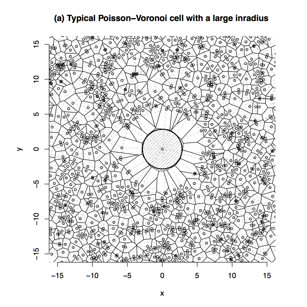
Refer to caption Refer to caption
Figure 2: Large inradius for a Poisson-Voronoi tessellation

4.2 Reciprocal of the inradius

In this example, we consider the large values of the reciprocal of the inradii for a Poisson-Voronoi tessellation in 𝐑dsuperscript𝐑𝑑\mathbf{R}^{d}. Equivalently, this consists of the small values of the inradii. Since (r(𝒞)<v)=1e2dκdvd𝑟𝒞𝑣1superscript𝑒superscript2𝑑subscript𝜅𝑑superscript𝑣𝑑\operatorname{\mathbb{P}}\left(\,r(\mathcal{C})<v\,\right)=1-e^{-2^{d}\kappa_{d}v^{d}}, we have ρ(r(𝒞)<vρ(τ))ρτ𝜌𝑟𝒞subscript𝑣𝜌𝜏𝜌𝜏\rho\cdot\mathbb{P}\left(\,r(\mathcal{C})<v_{\rho}(\tau)\right)\underset{\rho\rightarrow\infty}{\longrightarrow}\tau, when

vρ(τ):=21(κdρ)1/dτ1/d.assignsubscript𝑣𝜌𝜏superscript21superscriptsubscript𝜅𝑑𝜌1𝑑superscript𝜏1𝑑v_{\rho}(\tau):=2^{-1}(\kappa_{d}\rho)^{-1/d}\tau^{1/d}.

Here, we have written “r(𝒞)<vρ(τ)𝑟𝒞subscript𝑣𝜌𝜏r(\mathcal{C})<v_{\rho}(\tau)” instead of “r(𝒞)>vρ(τ)𝑟𝒞subscript𝑣𝜌𝜏r(\mathcal{C})>v_{\rho}(\tau)” in the probability because we consider the smallest inradii. Moreover, according to [7], we know that

(minxη𝐖ρr(Cη(x))vρ(τ))ρeτ/2.subscript𝑥𝜂subscript𝐖𝜌𝑟subscript𝐶𝜂𝑥subscript𝑣𝜌𝜏𝜌superscript𝑒𝜏2\mathbb{P}\left(\,\min_{x\in\eta\cap\mathbf{W}_{\rho}}r(C_{\eta}(x))\geq v_{\rho}(\tau)\right)\underset{\rho\rightarrow\infty}{\longrightarrow}e^{-\tau/2}.

We deduce that the extremal index of the reciprocal of the inradius of a Poisson-Voronoi tessellation exists and equals θ=1/2𝜃12\theta=1/2.

As in Section 4.1, we can easily simulate a Poisson-Voronoi tessellation in 𝐑2superscript𝐑2\mathbf{R}^{2}, conditional on the fact that rη{0}(0)<vexp(100)(1)5.441023superscript𝑟𝜂00subscript𝑣1001similar-to-or-equals5.44superscript1023r^{\eta\cup\{0\}}(0)<v_{\exp(100)}(1)\simeq 5.44\cdot 10^{-23}. The left part of Figure 3 provides a realization of a Poisson-Voronoi tessellation when rη{0}(0)<vexp(4)(1)0.0381superscript𝑟𝜂00subscript𝑣41similar-to-or-equals0.0381r^{\eta\cup\{0\}}(0)<v_{\exp(4)}(1)\simeq 0.0381 (here, we have taken the threshold vexp(4)(1)subscript𝑣41v_{\exp(4)}(1) instead of vexp(100)(1)subscript𝑣1001v_{\exp(100)}(1) for convenience). The fact that θ=1/2𝜃12\theta=1/2 can be explained by a trivial heuristic argument: if a cell minimizes the inradius, one of its neighbors has to do the same (see also the left part of Figure 3). Moreover, we can easily prove that the probability that there is more than one such a cell is negligible. Therefore clusters are necessarily of size 222, i.e. p2=1subscript𝑝21p_{2}=1. The right part of Figure 3 provides the box plots of the empirical distributions. In particular, for all simulations, we notice that there are always exactly two cells with a small inradius.
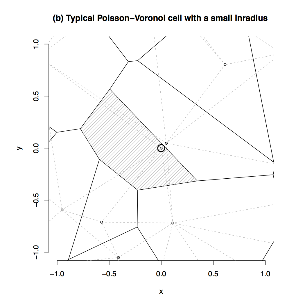
Refer to caption Refer to caption
Figure 3: Small inradius for a Poisson-Voronoi tessellation

4.3 Circumradius

For xη𝐑2𝑥𝜂superscript𝐑2x\in\eta\subset\mathbf{R}^{2}, we define the so-called circumradius of Cη(x)subscript𝐶𝜂𝑥C_{\eta}(x) as

Rη(x):=R(Cη(x)):=inf{r0:B(x,r)Cη(x)}.assignsuperscript𝑅𝜂𝑥𝑅subscript𝐶𝜂𝑥assigninfimumconditional-set𝑟0subscript𝐶𝜂𝑥𝐵𝑥𝑟R^{\eta}(x):=R(C_{\eta}(x)):=\inf\{r\geq 0:B(x,r)\supset C_{\eta}(x)\}.

According to [6], we know that

2vev(πR(𝒞)2>v,)4vev,2ve^{-v}\leq\mathbb{P}\left(\,\pi R(\mathcal{C})^{2}>v,\right)\leq 4ve^{-v},

for each v0.337𝑣0.337v\geq 0.337. Actually, simulations suggest that the upper bound above is the order of (πR(𝒞)2>v)𝜋𝑅superscript𝒞2𝑣\mathbb{P}\left(\pi R(\mathcal{C})^{2}>v\right) as v𝑣v goes to infinity (see Table 1 in [6]). If we assume that (πR(𝒞)2>v)ρavev𝜋𝑅superscript𝒞2𝑣𝜌similar-to𝑎𝑣superscript𝑒𝑣\mathbb{P}\left(\,\pi R(\mathcal{C})^{2}>v\,\right)\underset{\rho\rightarrow\infty}{\sim}ave^{-v} for some 2a42𝑎42\leq a\leq 4, we have ρ(R(𝒞)>vρ(τ))ρτ𝜌𝑅𝒞subscript𝑣𝜌𝜏𝜌𝜏\rho\cdot\mathbb{P}\left(\,R(\mathcal{C})>v_{\rho}(\tau)\right)\underset{\rho\rightarrow\infty}{\longrightarrow}\tau, when

vρ(τ):=π1/2(log(aρlogρτ1))1/2.assignsubscript𝑣𝜌𝜏superscript𝜋12superscript𝑎𝜌𝜌superscript𝜏112v_{\rho}(\tau):=\pi^{-1/2}\left(\log\left(a\rho\log\rho\tau^{-1}\right)\right)^{1/2}.

Thanks to (2.c) in [7], we know that

(maxxη𝐖ρRη(x)vρ(τ))ρeτ/a.subscript𝑥𝜂subscript𝐖𝜌superscript𝑅𝜂𝑥subscript𝑣𝜌𝜏𝜌superscript𝑒𝜏𝑎\mathbb{P}\left(\,\max_{x\in\eta\cap\mathbf{W}_{\rho}}R^{\eta}(x)\leq v_{\rho}(\tau)\right)\underset{\rho\rightarrow\infty}{\longrightarrow}e^{-\tau/a}.

Hence, provided that (πR(𝒞)2>v)ρavev𝜋𝑅superscript𝒞2𝑣𝜌similar-to𝑎𝑣superscript𝑒𝑣\mathbb{P}\left(\,\pi R(\mathcal{C})^{2}>v\,\right)\underset{\rho\rightarrow\infty}{\sim}ave^{-v}, the extremal index of the maximum of circumradius of a planar Poisson-Voronoi tessellation exists and should be equal to θ=1/a𝜃1𝑎\theta=1/a.

Now, we explain how we evaluate by simulation the value of the extremal index and the distribution p𝑝p. According to Lemma 1 in [13], we know that Rη{0}(0)>vsuperscript𝑅𝜂00𝑣R^{\eta\cup\{0\}}(0)>v if and only if there exists a disk of radius v𝑣v containing the origin on its boundary and no particle inside. Without loss of generality, we can assume that the disk, that contains the origin on its boundary and no particle inside, has its center on the x𝑥x-axis, since the Poisson point process is isotropic. Hence, we proceed as follows. First, we simulate a random variable Rbsubscript𝑅𝑏R_{b}, with distribution such that (πRb2>v)vbvev𝜋superscriptsubscript𝑅𝑏2𝑣𝑣similar-to𝑏𝑣superscript𝑒𝑣\operatorname{\mathbb{P}}\left(\,\pi R_{b}^{2}>v\,\right)\underset{v\rightarrow\infty}{\sim}bve^{-v}, with b=4𝑏4b=4, given that Rb>vexp(100)(1)5.81subscript𝑅𝑏subscript𝑣1001similar-to-or-equals5.81R_{b}>v_{\exp(100)}(1)\simeq 5.81. We have taken b=4𝑏4b=4 since we should have (πR(𝒞)2>v)v4vev𝜋𝑅superscript𝒞2𝑣𝑣similar-to4𝑣superscript𝑒𝑣\operatorname{\mathbb{P}}\left(\,\pi R(\mathcal{C})^{2}>v\,\right)\underset{v\rightarrow\infty}{\sim}4ve^{-v} as suggested in the simulations in [6]. However, this choice is arbitrary and does not have influence on the final result since the conditional distribution of Rbsubscript𝑅𝑏R_{b} does not depend on b𝑏b for high thresholds. Then, we generate a Voronoi tessellation induced by the point process ηB((R,0),R)c{0}subscript𝜂𝐵superscript𝑅0𝑅𝑐0\eta_{B((R,0),R)^{c}}\cup\{0\}, where ηB((R,0),R)csubscript𝜂𝐵superscript𝑅0𝑅𝑐\eta_{B((R,0),R)^{c}} is a Poisson point process of intensity measure 𝕀xB((R,0),R)cdxsubscript𝕀𝑥𝐵superscript𝑅0𝑅𝑐d𝑥\mathbb{I}_{x\in B((R,0),R)^{c}}\,\mathrm{d}x.

On the left part of Figure 4, we provide a simulation of the Palm version of the Poisson-Voronoi tessellation, given that R(𝒞)>vexp(100)(1)5.81𝑅𝒞subscript𝑣1001similar-to-or-equals5.81R(\mathcal{C})>v_{\exp(100)}(1)\simeq 5.81. We notice that the typical cell is very elongated and that the same fact holds for a large number of its connected cells. In particular, the size of a cluster of exceedances is random. On the right part of Figure 4, we provide the box plots of the empirical distributions. This time, the empirical distributions of the cluster size probabilities are not degenerated for k=3,,9𝑘39k=3,\ldots,9, and their interquartile ranges are quite large for k=3,4,5𝑘345k=3,4,5. We also notice that the empirical value of the extremal index is very concentrated around a value close to 1/4141/4. This confirms that if a𝑎a exists, it should be close to 4.

Refer to caption Refer to caption
Figure 4: Large circumradius for a Poisson-Voronoi tessellation

5 The case of the Poisson-Delaunay tessellation

The Poisson-Delaunay tessellation

Let χlf𝜒subscript𝑙𝑓\chi\in\mathcal{F}_{lf} be a locally finite subset of 𝐑dsuperscript𝐑𝑑\mathbf{R}^{d} such that each subset of size n<d+1𝑛𝑑1n<d+1 of points are affinely independent and no d+2𝑑2d+2 points lie on a sphere. If two points x,yχ𝑥𝑦𝜒x,y\in\chi are Voronoi neighbors, i.e. Cχ(x)Cχ(y)subscript𝐶𝜒𝑥subscript𝐶𝜒𝑦C_{\chi}(x)\cap C_{\chi}(y)\neq\varnothing, we connect these two points by an edge. The family of these edges defines a partition of 𝐑dsuperscript𝐑𝑑\mathbf{R}^{d} into simplices which is the so-called Delaunay tessellation. Another useful characterization of the Delaunay tessellation is the following: a simplex associated with d+1𝑑1d+1 points of χ𝜒\chi is a Delaunay simplex if and only if its circumball contains no point of χ𝜒\chi in its interior. Delaunay tessellations are very popular structures in computational geometry [1] and are extensively used in many areas such as surface reconstruction [9] or mesh generation [11].

For each cell C𝐶C of the Delaunay tessellation, the nucleus z(C)𝑧𝐶z(C) is defined as the center of the circumball of C𝐶C. The set of this nuclei is denoted by Z(χ)𝑍𝜒Z(\chi). Besides, for each zZ(χ)𝑧𝑍𝜒z\in Z(\chi), we denote by C(z)𝐶𝑧C(z) the Delaunay cell whose the center of its circumball is z𝑧z.

When χ=η𝜒𝜂\chi=\eta is a homogeneous Poisson point process, the family of these cells is the so-called Poisson-Delaunay tessellation. If we denote by γηsubscript𝛾𝜂\gamma_{\eta} the intensity of η𝜂\eta, then the intensity of the Poisson-Delaunay tessellation is γZ(η)=βd1γηsubscript𝛾𝑍𝜂superscriptsubscript𝛽𝑑1subscript𝛾𝜂\gamma_{Z(\eta)}=\beta_{d}^{-1}\cdot\gamma_{\eta}, where

βd:=(d3+d2)Γ(d22)Γd(d+12)Γ(d2+12)Γd(d+22)2d+1πd12.assignsubscript𝛽𝑑superscript𝑑3superscript𝑑2Γsuperscript𝑑22superscriptΓ𝑑𝑑12Γsuperscript𝑑212superscriptΓ𝑑𝑑22superscript2𝑑1superscript𝜋𝑑12\beta_{d}:=\frac{(d^{3}+d^{2})\Gamma\left(\frac{d^{2}}{2}\right)\Gamma^{d}\left(\frac{d+1}{2}\right)}{\Gamma\left(\frac{d^{2}+1}{2}\right)\Gamma^{d}\left(\frac{d+2}{2}\right)2^{d+1}\pi^{\frac{d-1}{2}}}.

In particular, if d=2𝑑2d=2, we have β2=1/2subscript𝛽212\beta_{2}=1/2. In the rest of the paper, we assume that γη=βdsubscript𝛾𝜂subscript𝛽𝑑\gamma_{\eta}=\beta_{d} to ensure that γZ(η)=1subscript𝛾𝑍𝜂1\gamma_{Z(\eta)}=1.

The typical cell of a Poisson-Delaunay tessellation can be made explicit as follows. Let Sd1:={x𝐑d:|x|=1}assignsuperscript𝑆𝑑1conditional-set𝑥superscript𝐑𝑑𝑥1S^{d-1}:=\{x\in\mathbf{R}^{d}:|x|=1\} be the unit sphere of 𝐑dsuperscript𝐑𝑑\mathbf{R}^{d} and, for u1:d+1(Sd1)d+1subscript𝑢:1𝑑1superscriptsuperscript𝑆𝑑1𝑑1u_{1:d+1}\in(S^{d-1})^{d+1}, let Δ(u1:d+1):=conv(u1,,ud+1)assignΔsubscript𝑢:1𝑑1𝑐𝑜𝑛𝑣subscript𝑢1subscript𝑢𝑑1\Delta(u_{1:d+1}):=conv(u_{1},\ldots,u_{d+1}). According to Miles (see e.g. Theorem 10.4.4 in [28]), for any bounded measurable function f:𝐑+×Sd1𝐑:𝑓subscript𝐑superscript𝑆𝑑1𝐑f:\mathbf{R}_{+}\times S^{d-1}\rightarrow\mathbf{R}, we have

𝔼[f(𝒞)]:=adγηd𝐑+Sd1Sd1a(u1:d+1)rd21eγηκdrdf(Δ(ru1:d+1))σ(du1:d+1)dr,assign𝔼delimited-[]𝑓𝒞subscript𝑎𝑑superscriptsubscript𝛾𝜂𝑑subscriptsubscript𝐑subscriptsuperscript𝑆𝑑1subscriptsuperscript𝑆𝑑1𝑎subscript𝑢:1𝑑1superscript𝑟superscript𝑑21superscript𝑒subscript𝛾𝜂subscript𝜅𝑑superscript𝑟𝑑𝑓Δ𝑟subscript𝑢:1𝑑1𝜎dsubscript𝑢:1𝑑1differential-d𝑟\mathbb{E}[f(\mathcal{C})]:=a_{d}\gamma_{\eta}^{d}\int_{\mathbf{R}_{+}}\int_{S^{d-1}}\cdots\int_{S^{d-1}}a(u_{1:d+1})r^{d^{2}-1}e^{-\gamma_{\eta}\kappa_{d}r^{d}}f(\Delta(ru_{1:d+1}))\sigma(\mathrm{d}u_{1:d+1})\mathrm{d}r, (5.1)

where ad:=βd/(d+1)assignsubscript𝑎𝑑subscript𝛽𝑑𝑑1a_{d}:=\beta_{d}/(d+1) and a(u1:d+1):=λd(Δ(u1:d+1))assign𝑎subscript𝑢:1𝑑1subscript𝜆𝑑Δsubscript𝑢:1𝑑1a(u_{1:d+1}):=\lambda_{d}\left(\Delta(u_{1:d+1})\right). The measure σ(du)𝜎d𝑢\sigma(\mathrm{d}u) is the uniform distribution on Sd1superscript𝑆𝑑1S^{d-1} with normalization σ(Sd1)=ωd1𝜎superscript𝑆𝑑1subscript𝜔𝑑1\sigma(S^{d-1})=\omega_{d-1}, where ωd1:=dκdassignsubscript𝜔𝑑1𝑑subscript𝜅𝑑\omega_{d-1}:=d\kappa_{d} is the area of the unit sphere and σ(du1:d+1):=i=1d+1σ(dui)assign𝜎dsubscript𝑢:1𝑑1superscriptsubscripttensor-product𝑖1𝑑1𝜎dsubscript𝑢𝑖\sigma(\mathrm{d}u_{1:d+1}):=\bigotimes_{i=1}^{d+1}\sigma(\mathrm{d}u_{i}). Hence, the typical satisifes the equality in distribution 𝒞=𝒟Δ(RU1:d+1)𝒞𝒟Δ𝑅subscript𝑈:1𝑑1\mathcal{C}\overset{\mathcal{D}}{=}\Delta(RU_{1:d+1}), where R>0𝑅0R>0 and U1:d+1(Sd1)d+1subscript𝑈:1𝑑1superscriptsuperscript𝑆𝑑1𝑑1U_{1:d+1}\in(S^{d-1})^{d+1} are two independent random variables whose the distributions are provided in (1.1).

The extremes of the Poisson-Delaunay tessellation

Let g𝑔g be a geometric characteristic such that (1.6) holds. As for a Poisson-Voronoi tessellation, we consider the point process of normalized exceedances, say

Ψη(τ):=ρ1/d{zZ(η):g(C(z))>vρ(τ)}.assignsuperscriptΨ𝜂𝜏superscript𝜌1𝑑conditional-set𝑧𝑍𝜂𝑔𝐶𝑧subscript𝑣𝜌𝜏\Psi^{\eta}(\tau):=\rho^{-1/d}\cdot\left\{z\in Z(\eta):g(C(z))>v_{\rho}(\tau)\right\}.

For any Borel subset B𝐑d𝐵superscript𝐑𝑑B\subset\mathbf{R}^{d}, we write ΨBη(τ):=Ψη(τ)(ρ1/dB)assignsubscriptsuperscriptΨ𝜂𝐵𝜏superscriptΨ𝜂𝜏superscript𝜌1𝑑𝐵\Psi^{\eta}_{B}(\tau):=\Psi^{\eta}(\tau)\cap(\rho^{-1/d}B). We also let Ψη,0(τ)superscriptΨ𝜂0𝜏\Psi^{\eta,0}(\tau) be the Palm version of Ψη(τ)superscriptΨ𝜂𝜏\Psi^{\eta}(\tau) and ΨBη,0(τ)=Ψη,0(τ)BsuperscriptsubscriptΨ𝐵𝜂0𝜏superscriptΨ𝜂0𝜏𝐵\Psi_{B}^{\eta,0}(\tau)=\Psi^{\eta,0}(\tau)\cap B. In the rest of the paper, the quantity pk,B(τ)subscript𝑝𝑘𝐵𝜏p_{k,B}(\tau) refers to as the probability that there exist k𝑘k exceedance cells in B𝐵B conditional on the fact that the typical cell is an exceedance, i.e. pk,B(τ):=(#ψBη,0(τ)=k)assignsubscript𝑝𝑘𝐵𝜏#superscriptsubscript𝜓𝐵𝜂0𝜏𝑘p_{k,B}(\tau):=\operatorname{\mathbb{P}}\left(\,\#\psi_{B}^{\eta,0}(\tau)=k\,\right). In the same spirit as Lemma 2, we provide below an explicit characterization of this probability.

Proposition 8.

Let 𝒜𝒜\mathcal{A} be a Borel subset in lfsubscript𝑙𝑓\mathcal{F}_{lf}. Then

(Ψη,0(τ)𝒜)=(Ψη𝐑dB(0,R){RU1:d+1}(τ)𝒜|g(Δ(RU1:d+1))>vρ(τ)).superscriptΨ𝜂0𝜏𝒜superscriptΨsubscript𝜂superscript𝐑𝑑𝐵0𝑅𝑅subscript𝑈:1𝑑1𝜏𝒜ket𝑔Δ𝑅subscript𝑈:1𝑑1subscript𝑣𝜌𝜏\mathbb{P}\left(\,\Psi^{\eta,0}(\tau)\in\mathcal{A}\,\right)=\mathbb{P}\left(\,\left.\Psi^{\eta_{\mathbf{R}^{d}\setminus B(0,R)}\cup\{RU_{1:d+1}\}}(\tau)\in\mathcal{A}\right|g(\Delta(RU_{1:d+1}))>v_{\rho}(\tau)\right).

Therefore, for any B𝐑d𝐵superscript𝐑𝑑B\subset\mathbf{R}^{d},

pk,B(τ)=(#ΨBη𝐑dB(0,R){RU1:d+1}(τ)=k|g(Δ(RU1:d+1))>vρ(τ)).subscript𝑝𝑘𝐵𝜏#superscriptsubscriptΨ𝐵subscript𝜂superscript𝐑𝑑𝐵0𝑅𝑅subscript𝑈:1𝑑1𝜏𝑘ket𝑔Δ𝑅subscript𝑈:1𝑑1subscript𝑣𝜌𝜏p_{k,B}(\tau)=\mathbb{P}\left(\,\left.\#\Psi_{B}^{\eta_{\mathbf{R}^{d}\setminus B(0,R)}\cup\{RU_{1:d+1}\}}(\tau)=k\right|g(\Delta(RU_{1:d+1}))>v_{\rho}(\tau)\right).

Proof Let A𝐑d𝐴superscript𝐑𝑑A\subset\mathbf{R}^{d} be such that λd(A)=1subscript𝜆𝑑𝐴1\lambda_{d}(A)=1. It follows from the definition of the Palm distribution of the point process Ψη(τ)superscriptΨ𝜂𝜏\Psi^{\eta}(\tau), that

(Ψη,0(τ)𝒜):=1γΨη(τ)𝔼[zΨη(τ)A𝕀(Ψη(τ)z)𝒜]=1γΨη(τ)𝔼[{x1:d+1}η𝕀(Ψη(τ)ρ1/dz(x1:d+1))𝒜𝕀z(x1:d+1)Z(η)𝐀ρ],assignsuperscriptΨ𝜂0𝜏𝒜1subscript𝛾superscriptΨ𝜂𝜏𝔼delimited-[]subscript𝑧superscriptΨ𝜂𝜏𝐴subscript𝕀superscriptΨ𝜂𝜏𝑧𝒜1subscript𝛾superscriptΨ𝜂𝜏𝔼delimited-[]subscriptsubscript𝑥:1𝑑1𝜂subscript𝕀superscriptΨ𝜂𝜏superscript𝜌1𝑑𝑧subscript𝑥:1𝑑1𝒜subscript𝕀𝑧subscript𝑥:1𝑑1𝑍𝜂subscript𝐀𝜌\begin{split}\mathbb{P}\left(\Psi^{\eta,0}(\tau)\in\mathcal{A}\,\right)&:=\frac{1}{\gamma_{\Psi^{\eta}(\tau)}}\mathbb{E}\left[\,\sum_{z\in\Psi^{\eta}(\tau)\cap A}\mathbb{I}_{(\Psi^{\eta}(\tau)-z)\in\mathcal{A}}\right]\\ &=\frac{1}{\gamma_{\Psi^{\eta}(\tau)}}\mathbb{E}\left[\,\sum_{\{x_{1:d+1}\}\subset\eta}\mathbb{I}_{(\Psi^{\eta}(\tau)-\rho^{1/d}z(x_{1:d+1}))\in\mathcal{A}}\,\mathbb{I}_{z(x_{1:d+1})\in Z(\eta)\cap\mathbf{A}_{\rho}}\,\,\right],\end{split}

where z(x1:d+1)𝑧subscript𝑥:1𝑑1z(x_{1:d+1}) is the center of the circumball of the simplex Δ(x1:d+1)Δsubscript𝑥:1𝑑1\Delta(x_{1:d+1}). According to the Slivnyak-Mecke formula and the Blaschke-Petkantschin formula (e.g. Theorem 7.3.1 in [28]) that

(Ψη,0(τ)𝒜)=γηd+1d!γΨη(τ)(d+1)!𝐀ρ𝐑+Sd+1rd21a(u1:d+1)×((Ψη(τ)ρ1/dz)𝒜,ηB(z,r)=)𝕀g(z+Δ(ru1:d+1))>vρ(τ)σ(du1:d+1)drdz.superscriptΨ𝜂0𝜏𝒜superscriptsubscript𝛾𝜂𝑑1𝑑subscript𝛾superscriptΨ𝜂𝜏𝑑1subscriptsubscript𝐀𝜌subscriptsubscript𝐑subscriptsuperscript𝑆𝑑1superscript𝑟superscript𝑑21𝑎subscript𝑢:1𝑑1formulae-sequencesuperscriptΨ𝜂𝜏superscript𝜌1𝑑𝑧𝒜𝜂𝐵𝑧𝑟subscript𝕀𝑔𝑧Δ𝑟subscript𝑢:1𝑑1subscript𝑣𝜌𝜏𝜎dsubscript𝑢:1𝑑1d𝑟d𝑧\mathbb{P}\left(\Psi^{\eta,0}(\tau)\in\mathcal{A}\right)=\frac{\gamma_{\eta}^{d+1}d!}{\gamma_{\Psi^{\eta}(\tau)}(d+1)!}\int_{\mathbf{A}_{\rho}}\int_{\mathbf{R}_{+}}\int_{S^{d+1}}r^{d^{2}-1}a(u_{1:d+1})\\ \times\mathbb{P}\left((\Psi^{\eta}(\tau)-\rho^{1/d}z)\in\mathcal{A},\eta\cap B(z,r)=\varnothing\,\right)\mathbb{I}_{g(z+\Delta(ru_{1:d+1}))>v_{\rho}(\tau)}\,\sigma(\mathrm{d}u_{1:d+1})\mathrm{d}r\mathrm{d}z.

Since η𝜂\eta is stationary and since g𝑔g is translation-invariant, the integrand does not depend on z𝑧z. Integrating over z𝐀ρ𝑧subscript𝐀𝜌z\in\mathbf{A}_{\rho}, and using the fact that λd(𝐀ρ)=ρsubscript𝜆𝑑subscript𝐀𝜌𝜌\lambda_{d}(\mathbf{A}_{\rho})=\rho, we get

(Ψη,0(τ)𝒜)=γηd+1ργΨη(τ)(d+1)𝐑+Sd+1rd21a(u1:d+1)×(Ψη(τ)𝒜,ηB(0,r)=)𝕀g(Δ(ru1:d+1))>vρ(τ)σ(du1:d+1)dr.superscriptΨ𝜂0𝜏𝒜superscriptsubscript𝛾𝜂𝑑1𝜌subscript𝛾superscriptΨ𝜂𝜏𝑑1subscriptsubscript𝐑subscriptsuperscript𝑆𝑑1superscript𝑟superscript𝑑21𝑎subscript𝑢:1𝑑1formulae-sequencesuperscriptΨ𝜂𝜏𝒜𝜂𝐵0𝑟subscript𝕀𝑔Δ𝑟subscript𝑢:1𝑑1subscript𝑣𝜌𝜏𝜎dsubscript𝑢:1𝑑1d𝑟\mathbb{P}\left(\,\Psi^{\eta,0}(\tau)\in\mathcal{A}\right)=\frac{\gamma_{\eta}^{d+1}\rho}{\gamma_{\Psi^{\eta}(\tau)}(d+1)}\int_{\mathbf{R}_{+}}\int_{S^{d+1}}r^{d^{2}-1}a(u_{1:d+1})\\ \times\mathbb{P}\left(\Psi^{\eta}(\tau)\in\mathcal{A},\eta\cap B(0,r)=\varnothing\,\right)\mathbb{I}_{g(\Delta(ru_{1:d+1}))>v_{\rho}(\tau)}\,\sigma(\mathrm{d}u_{1:d+1})\mathrm{d}r.

We give below an explicit representation for the integrand. Let ηB(0,r)subscript𝜂𝐵0𝑟\eta_{B(0,r)} and η𝐑dB(0,r)subscript𝜂superscript𝐑𝑑𝐵0𝑟\eta_{\mathbf{R}^{d}\setminus B(0,r)} be two independent Poisson point processes with intensity measures γη𝕀xB(0,R)dxsubscript𝛾𝜂subscript𝕀𝑥𝐵0𝑅d𝑥\gamma_{\eta}\mathbb{I}_{x\in B(0,R)}\,\mathrm{d}x and γη𝕀x𝐑dB(0,r)dxsubscript𝛾𝜂subscript𝕀𝑥superscript𝐑𝑑𝐵0𝑟d𝑥\gamma_{\eta}\mathbb{I}_{x\in\mathbf{R}^{d}\setminus B(0,r)}\,\mathrm{d}x respectively. We know that

η=𝒟ηB(0,r)η𝐑dB(0,r).𝜂𝒟subscript𝜂𝐵0𝑟subscript𝜂superscript𝐑𝑑𝐵0𝑟\eta\overset{\mathcal{D}}{=}\eta_{B(0,r)}\cup\eta_{\mathbf{R}^{d}\setminus B(0,r)}.

This gives

(Ψη(τ)𝒜,ηB(0,r)=)=(Ψη𝐑dB(0,r){ru1:d+1}(τ)𝒜,ηB(0,r)B(0,r)=)=eγηκdrd(Ψη𝐑dB(0,r){ru1:d+1}(τ)𝒜).formulae-sequencesuperscriptΨ𝜂𝜏𝒜𝜂𝐵0𝑟formulae-sequencesuperscriptΨsubscript𝜂superscript𝐑𝑑𝐵0𝑟𝑟subscript𝑢:1𝑑1𝜏𝒜subscript𝜂𝐵0𝑟𝐵0𝑟superscript𝑒subscript𝛾𝜂subscript𝜅𝑑superscript𝑟𝑑superscriptΨsubscript𝜂superscript𝐑𝑑𝐵0𝑟𝑟subscript𝑢:1𝑑1𝜏𝒜\begin{split}\mathbb{P}\left(\Psi^{\eta}(\tau)\in\mathcal{A},\eta\cap B(0,r)=\varnothing\,\right)&=\mathbb{P}\left(\,\Psi^{\eta_{\mathbf{R}^{d}\setminus B(0,r)}\cup\{ru_{1:d+1}\}}(\tau)\in\mathcal{A},\eta_{B(0,r)}\cap B(0,r)=\varnothing\,\right)\\ &=e^{-\gamma_{\eta}\kappa_{d}r^{d}}\mathbb{P}\left(\,\Psi^{\eta_{\mathbf{R}^{d}\setminus B(0,r)}\cup\{ru_{1:d+1}\}}(\tau)\in\mathcal{A}\,\right).\end{split}

Hence,

(Ψη,0(τ)𝒜)=γηd+1ργΨη(τ)(d+1)𝐑+Sd+1rd21a(u1:d+1)×eγηκdrd(Ψη𝐑dB(0,r){ru1:d+1}(τ)𝒜)σ(du1:d+1)dr.superscriptΨ𝜂0𝜏𝒜superscriptsubscript𝛾𝜂𝑑1𝜌subscript𝛾superscriptΨ𝜂𝜏𝑑1subscriptsubscript𝐑subscriptsuperscript𝑆𝑑1superscript𝑟superscript𝑑21𝑎subscript𝑢:1𝑑1superscript𝑒subscript𝛾𝜂subscript𝜅𝑑superscript𝑟𝑑superscriptΨsubscript𝜂superscript𝐑𝑑𝐵0𝑟𝑟subscript𝑢:1𝑑1𝜏𝒜𝜎dsubscript𝑢:1𝑑1d𝑟\mathbb{P}\left(\,\Psi^{\eta,0}(\tau)\in\mathcal{A}\right)=\frac{\gamma_{\eta}^{d+1}\rho}{\gamma_{\Psi^{\eta}(\tau)}(d+1)}\int_{\mathbf{R}_{+}}\int_{S^{d+1}}r^{d^{2}-1}a(u_{1:d+1})\\ \times e^{-\gamma_{\eta}\kappa_{d}r^{d}}\mathbb{P}\left(\Psi^{\eta_{\mathbf{R}^{d}\setminus B(0,r)}\cup\{ru_{1:d+1}\}}(\tau)\in\mathcal{A}\,\right)\sigma(\mathrm{d}u_{1:d+1})\mathrm{d}r.

Moreover, we know that γΨη(τ)=ρ(g(𝒞)>vρ(τ))subscript𝛾superscriptΨ𝜂𝜏𝜌𝑔𝒞subscript𝑣𝜌𝜏\gamma_{\Psi^{\eta}(\tau)}=\rho\mathbb{P}\left(g(\mathcal{C})>v_{\rho}(\tau)\right) and that γη=(d+1)adsubscript𝛾𝜂𝑑1subscript𝑎𝑑\gamma_{\eta}=(d+1)a_{d}. Then, we get

(Ψη,0(τ)𝒜)=adγηd(g(𝒞)>vρ(τ))𝐑+Sd+1rd21a(u1:d+1)×eγηκdrd(Ψη𝐑dB(0,r){ru1:d+1}𝒜)σ(du1:d+1)dr.superscriptΨ𝜂0𝜏𝒜subscript𝑎𝑑superscriptsubscript𝛾𝜂𝑑𝑔𝒞subscript𝑣𝜌𝜏subscriptsubscript𝐑subscriptsuperscript𝑆𝑑1superscript𝑟superscript𝑑21𝑎subscript𝑢:1d1superscript𝑒subscript𝛾𝜂subscript𝜅𝑑superscript𝑟𝑑superscriptΨsubscript𝜂superscript𝐑𝑑𝐵0𝑟𝑟subscript𝑢:1𝑑1𝒜𝜎dsubscript𝑢:1𝑑1d𝑟\mathbb{P}\left(\,\Psi^{\eta,0}(\tau)\in\mathcal{A}\right)=\frac{a_{d}\gamma_{\eta}^{d}}{\mathbb{P}\left(\,g(\mathcal{C})>v_{\rho}(\tau)\right)}\int_{\mathbf{R}_{+}}\int_{S^{d+1}}r^{d^{2}-1}a(u_{1:\mathrm{d}+1})\\ \times e^{-\gamma_{\eta}\kappa_{d}r^{d}}\mathbb{P}\left(\,\Psi^{\eta_{\mathbf{R}^{d}\setminus B(0,r)}\cup\{ru_{1:d+1}\}}\in\mathcal{A}\,\right)\sigma(\mathrm{d}u_{1:d+1})\mathrm{d}r.

This proves the first equality in Proposition 8 since 𝒞=𝒟Δ(RU1:d+1)𝒞𝒟Δ𝑅subscript𝑈:1𝑑1\mathcal{C}\overset{\mathcal{D}}{=}\Delta(RU_{1:d+1}). The second equality is a direct consequence of the first one. \square

We think that Theorem 4 can be adapted in the context of a Poisson-Delaunay tessellation. To do it, we have to replace the point process Φη(τ)superscriptΦ𝜂𝜏\Phi^{\eta}(\tau) by the point process Ψη(τ)superscriptΨ𝜂𝜏\Psi^{\eta}(\tau) and we have to use the characterization of the probability pk,𝔔ρ(τ0)subscript𝑝𝑘subscript𝔔𝜌subscript𝜏0p_{k,\mathfrak{Q}_{\rho}}(\tau_{0}) as described in the above proposition. We can easily extend Lemma 1 and adapt Condition (C) in the particular setting of a Poisson-Delaunay tessellation. However, the main difficulty to adapt Theorem 4 focuses on an analogous version of Proposition 3 since its proof seems very technical. We give below a numerical illustration which confirms that Theorem 4 should be true for a Poisson-Delaunay tessellation.

A numerical illustration

Let mPDTsubscript𝑚𝑃𝐷𝑇m_{PDT} be a Poisson-Delaunay tessellation generated by a Poisson point process η𝜂\eta in 𝐑dsuperscript𝐑𝑑\mathbf{R}^{d} with intensity γη=βdsubscript𝛾𝜂subscript𝛽𝑑\gamma_{\eta}=\beta_{d}. For each cell CmPDT𝐶subscript𝑚𝑃𝐷𝑇C\in m_{PDT}, we consider the so-called circumcenter of C𝐶C defined as

R(C):=inf{R0:CB(z,R),zd}.assign𝑅𝐶infimumconditional-set𝑅0formulae-sequence𝐶𝐵𝑧𝑅𝑧superscript𝑑R(C):=\inf\{R\geq 0:C\subset B(z,R),z\in\mathbb{R}^{d}\}.

According to (5.1)italic-(5.1italic-)\eqref{def:TypicalDelaunay}, the random variable κdR(𝒞)dsubscript𝜅𝑑𝑅superscript𝒞𝑑\kappa_{d}R(\mathcal{C})^{d} is Gamma distributed with parameters (d,βd)𝑑subscript𝛽𝑑(d,\beta_{d}). A Taylor expansion of (R(𝒞)>v)𝑅𝒞𝑣\mathbb{P}\left(R(\mathcal{C})>v\right) as v𝑣v goes to infinity (e.g. Equation (3.14) in [10]), shows that ρ(R(𝒞)>vρ(τ))ρτ𝜌𝑅𝒞subscript𝑣𝜌𝜏𝜌𝜏\rho\cdot\mathbb{P}\left(\,R(\mathcal{C})>v_{\rho}(\tau)\right)\underset{\rho\rightarrow\infty}{\longrightarrow}\tau, when

vρ(τ):=(κdβd)1/d(log([(d1)!]1ρlog(βdρ)d1τ1))1/d.v_{\rho}(\tau):=(\kappa_{d}\beta_{d})^{-1/d}\cdot\left(\log\left([(d-1)!]^{-1}\rho\log(\beta_{d}\rho)^{d-1}\tau^{-1}\right)\right)^{1/d}.

Moreover, with standard arguments, we can easily show that the maximum of circumradii of Delaunay cells maxCmPDT,z(C)𝐖ρR(C)subscriptabsentformulae-sequence𝐶subscript𝑚𝑃𝐷𝑇𝑧𝐶subscript𝐖𝜌𝑅𝐶\max_{\underset{}{C\in m_{PDT},z(C)\in\mathbf{W}_{\rho}}}R(C) has the same asymptotic behavior as the maximum of circumradii of the associated Voronoi cells maxxη𝐖ρR(Cη(x))subscript𝑥𝜂subscript𝐖𝜌𝑅subscript𝐶𝜂𝑥\max_{x\in\eta\cap\mathbf{W}_{\rho}}R(C_{\eta}(x)). Besides, according to (2c) in [10], we know that

(maxxη𝐖ρR(Cη(x))(κdβd)1/d(log(αdβdρlog(βdρ)d1τ1))1/d)ρeτ,\operatorname{\mathbb{P}}\left(\,\max_{x\in\eta\cap\mathbf{W}_{\rho}}R(C_{\eta}(x))\leq(\kappa_{d}\beta_{d})^{-1/d}\left(\log\left(\alpha_{d}\beta_{d}\rho\log(\beta_{d}\rho)^{d-1}\tau^{-1}\right)\right)^{1/d}\,\right)\underset{\rho\rightarrow\infty}{\longrightarrow}e^{-\tau},

where αd:=1d!(π1/2Γ(d2+1)Γ(d+12))d1assignsubscript𝛼𝑑1𝑑superscriptsuperscript𝜋12Γ𝑑21Γ𝑑12𝑑1\alpha_{d}:=\frac{1}{d!}\left(\frac{\pi^{1/2}\Gamma\left(\frac{d}{2}+1\right)}{\Gamma\left(\frac{d+1}{2}\right)}\right)^{d-1}. It follows that

(maxCmPDT,z(C)𝐖ρR(C)vρ(τ))ρeθdτ,\mathbb{P}\left(\,\max_{\underset{z(C)\in\mathbf{W}_{\rho}}{C\in m_{PDT},}}R(C)\leq v_{\rho}(\tau)\,\right)\underset{\rho\rightarrow\infty}{\longrightarrow}e^{-\theta_{d}\tau},

where

θd:=αdβd(d1)!=(d3+d2)Γ(d22)Γ(d+12)dΓ(d2+12)Γ(d+22)2d+1.assignsubscript𝜃𝑑subscript𝛼𝑑subscript𝛽𝑑𝑑1superscript𝑑3superscript𝑑2Γsuperscript𝑑22Γ𝑑12𝑑Γsuperscript𝑑212Γ𝑑22superscript2𝑑1\theta_{d}:=\alpha_{d}\beta_{d}(d-1)!=\frac{(d^{3}+d^{2})\Gamma\left(\frac{d^{2}}{2}\right)\Gamma\left(\frac{d+1}{2}\right)}{d\Gamma\left(\frac{d^{2}+1}{2}\right)\Gamma\left(\frac{d+2}{2}\right)2^{d+1}}.

In particular, when d=1,2,3𝑑123d=1,2,3, the extremal index equals θ1=1subscript𝜃11\theta_{1}=1, θ2=1/2subscript𝜃212\theta_{2}=1/2 and θ3=35/128subscript𝜃335128\theta_{3}=35/128 respectively.

Now, we explain how we evaluate by simulation the value of the extremal index and the distribution p𝑝p when d=2𝑑2d=2. First, we simulate a random variable R𝑅R such that πR2𝜋superscript𝑅2\pi R^{2} is Gamma distributed with parameters (2,1/2)212(2,1/2), given that R>vexp(100)(1)8.16𝑅subscript𝑣1001similar-to-or-equals8.16R>v_{\exp(100)}(1)\simeq 8.16. Then we simulate a typical cell 𝒞𝒞\mathcal{C}, with circumradius R𝑅R, by using the method described in [17]. The Poisson-Delaunay tessellation which is generated is induced by the point process ηB(0,2R)c{0}subscript𝜂𝐵superscript02𝑅𝑐0\eta_{B(0,2R)^{c}}\cup\{0\}, where ηB(0,2R)csubscript𝜂𝐵superscript02𝑅𝑐\eta_{B(0,2R)^{c}} is a Poisson point process with intensity measure 𝕀xB(0,2R)cdxsubscript𝕀𝑥𝐵superscript02𝑅𝑐d𝑥\mathbb{I}_{x\in B(0,2R)^{c}}\,\mathrm{d}x (see Proposition 8).

On the left part of Figure 5, we provide a simulation of the Palm version of the Poisson-Delaunay tessellation given that the typical cell has a circumradius larger than 8.168.168.16. The number of neighbors of the typical cells which are exceedances is random. The right part of Figure 5 provides the box plots of the empirical probabilities. Notice that these empirical distributions are not degenerated for k=1,,8𝑘18k=1,\ldots,8. Their interquartile ranges are not so important as for the circumradii of the Poisson-Voronoi tessellation, but the spread of the empirical distribution of the extremal index is larger. Besides, the empirical value of the extremal index is very concentrated around a value close to 1/2121/2, which is the theoretical value of θ𝜃\theta.

Refer to caption Refer to caption
Figure 5: Large circumradius for a Poisson-Delaunay tessellation

References

  • [1] F. Aurenhammer, R. Klein, D.T. Lee. Voronoi diagrams and Delaunay triangulations. World Scientific, (8): 2013.
  • [2] F. Avram and D. Bertsimas. On central limit theorem in geometrical probability. The Annals of Applied Probability, 3(4):1033–1046, 1993.
  • [3] F. Baccelli and B. Blaszczyszyn. Stochastic geometry and wireless networks. Volume 2: Applications. Foundations and Trends in Networking : Vol. 1: Theory, Vol. 2: Applications No 1-2, 2009.
  • [4] B. Basrak and J. Segers. Regularly varying multivariate time series. Stochastic Process. Appl., 119(4):1055–1080, 2009.
  • [5] V. Baumstark and G. Last. Some distributional results for Poisson-Voronoi tessellations. Adv. in Appl. Probab., 39(1):16–40, 2007.
  • [6] P. Calka. The distributions of the smallest disks containing the Poisson-Voronoi typical cell and the Crofton cell in the plane. Adv. in Appl. Probab., 34(4):702–717, 2002.
  • [7] P. Calka and N. Chenavier. Extreme values for characteristic radii of a Poisson-Voronoi tessellation. Extremes, 17(3):359–385, 2014.
  • [8] P. Calka and T. Schreiber. Limit theorems for the typical Poisson-Voronoi cell and the Crofton cell with a large inradius. Ann. Probab., 33(4):1625–1642, 2005.
  • [9] F. Cazals and J. Giesen. Delaunay triangulation based surface reconstruction. Effective computational geometry for curves and surfaces, 231–276, 2006.
  • [10] N. Chenavier. A general study of extremes of stationary tessellations with examples. Stochastic Process. Appl., 124(9):2917–2953, 2014.
  • [11] S.W. Cheng, T.K. Dey, J. Shewchuk. Delaunay mesh generation. CRC Press, 2012.
  • [12] H. Ferreira and L. Pereira. Point processes of exceedances by random fields. J. Statist. Plann., 142(3):773–779, 2012.
  • [13] S. G. Foss and S. A. Zuyev. On a Voronoi aggregative process related to a bivariate Poisson process. Adv. in Appl. Probab., 28(4):965–981, 1996.
  • [14] L. Heinrich and L. Muche. Second-order properties of the point process of nodes in a stationary Voronoi tessellation. Math. Nachr., 281(3):350–375, 2008.
  • [15] L. Hsing, J. Hüsler, and M. R. Leadbetter. On the exceedance point process for a stationary sequence. Probab. Theory Related Fields, 78(1):97–112, 1988.
  • [16] D. Hug, M. Reitzner, and R. Schneider. Large Poisson–Voronoi cells and Crofton cells. Adv. in Appl. Probab, 36: 667–690, 2004.
  • [17] D.G. Kendall, D. G. Random Delaunay simplexes in 𝐑msuperscript𝐑𝑚{\bf R}^{m}. J. Statist. Plann. Inference, 25(3):225–234, 1990.
  • [18] M.R. Leadbetter, M. R. Extremes and local dependence in stationary sequences. Z. Wahrsch. Verw. Gebiete, 65: 291–306, 1983.
  • [19] R. E. Miles. The various aggregates of random polygons determined by random lines in a plane. Adv. Math. 10: 256–290, 1973.
  • [20] J. Møller. Random tessellations in Rdsuperscript𝑅𝑑R^{d}. Adv. in Appl. Probab., 21(1):37–73, 1989.
  • [21] L. Muche. The Poisson-Voronoi tessellation: relationships for edges. Adv. in Appl. Probab., 37(2):279–296, 2005.
  • [22] A. Okabe, B. Boots, K. Sugihara, and S. N. Chiu. Spatial tessellations: concepts and applications of Voronoi diagrams. Wiley Series in Probability and Statistics. John Wiley & Sons Ltd., Chichester, second edition, 2000.
  • [23] G.Pagès, G. and B. Wilbertz. Optimal Delaunay and Voronoi quantization schemes for pricing American style options. Springer Proc. Math. 12:171–213, 2012.
  • [24] R. Perfekt. Extremal behaviour of stationary Markov chains with applications. Ann. Appl. Probab., 4(2):529–548, 1994.
  • [25] A. Poupon. Voronoi and Voronoi-related tessellations in studies of protein structure and interaction. Current Opinion in Structural Biology, 14(2):233–241, 2004.
  • [26] C. Y. Robert. Inference for the limiting cluster size distribution of extreme values. Ann. Statist., 37(1):271–310, 2009.
  • [27] H. Rootzen. Maxima and exceedances of stationary Markov chain. Adv. Appli. Probab, 1988.
  • [28] R. Schneider and W. Weil. Stochastic and integral geometry. Probability and its Applications (New York). Springer-Verlag, Berlin, 2008.
  • [29] R.L. Smith, and I. Weissman. Estimating the extremal index. J. Roy. Statist. Soc. Ser. B, 56: 56, 515–528, 1994.
  • [30] R.L. Smith. A counterexample concerning the extremal index. Adv. in Appl. Probab., 20:681–683, 1988.
  • [31] D. Stoyan, W. Kendall, and J. Mecke, J. Stochastic Geometry and its applications. Wiley, 2008.
  • [32] L. Zaninetti. The oscillating behavior of the pair correlation function in galaxies. Applied Physics Research, 1:35–46, 2014.