Adaptive Gray World-Based Color Normalization of Thin Blood Film Images

Abstract

This paper presents an effective color normalization method for thin blood film images of peripheral blood specimens. Thin blood film images can easily be separated to foreground (cell) and background (plasma) parts. The color of the plasma region is used to estimate and reduce the differences arising from different illumination conditions. A second stage normalization based on the database-gray world algorithm transforms the color of the foreground objects to match a reference color character. The quantitative experiments demonstrate the effectiveness of the method and its advantages against two other general purpose color correction methods: simple gray world and Retinex.

Index Terms—  blood cells, color normalization, gray world, Retinex, thin blood film,

1 Introduction

Microscopy examination of blood specimens is still the gold standard for the diagnosis of several diseases. However, it is usually a tedious and subjective task to perform manually. On the other hand, automated diagnosis systems aim to replicate diagnostic expertise by specifically tailored image processing, analysis, and pattern recognition algorithms [1]. However, image variations that are commonly neglected by humans generate problems for automated algorithms.

An image acquired from a stained blood specimen (thick or thin) using a conventional light microscope can have several conditions which may affect the observed colors of the cells, plasma (background), and stained objects. These conditions may be due to the microscope components such as: different color characteristics of light sources, intensity adjustments, or color filters; use of different cameras or different settings in the same camera such as exposure, aperture diagram, or white balance settings. It is possible to reduce these effects by calibration. However, variations can also be caused in slide preparation such as use of different stain concentrations, exposure to different staining durations, or non-uniform staining.

There are various studies addressing the calibration and color constancy issues for general imaging [2]. However, the field literature for microscope imaging is quite limited. The general purpose methods of color correction is not appropriate for microscope imaging because first the Lambertian surface model does not fit to microscope imaging, 2) the use of the reference color charts are not practical. Simply, because the sensor (or human eye) does not receive the light reflecting from a surface; it is the attenuated light that is left from the object’s (i.e. specimen’s) absorption. In fact, image formation of the stained slides with light microscopes can be appropriately modeled with the “Beer-Lambert Law”, which states that there is a linear relationship between the concentration, thickness of illuminated media, and the “absorbance” [3]. In addition, the reference color patches (as proposed for other medical imaging applications, e.g. [4], is not practical for microscopes. Moreover, there is still the human factor in preparation of the slides which results in non-standard and inhomogeneous staining concentrations and colors [5].

The problem of non-standard preparation of the slides (specimen) was addressed in [6]. To correct under/over staining conditions of the slide, Abe et al. obtained the spectral transmittance by a multi- spectral camera, and mathematically modeled the relation between the transmittance and the amount of stain (dye) for each pixel using the Beer-Lambert Law and Wiener inverse estimation. However, the method required a multi-spectral camera to operate, and variations caused by different light sources were not addressed.

In [7] we proposed a practical method which exploits the special characteristics of the peripheral thin blood film images that are easily separable to foreground and background regions. However, the method was presented briefly as a procedure and no quantifiable evaluation was given. In this study, we reformulate this color normalization algorithm, and compare it to two other general purpose color correction algorithms: simple gray world [2] and Retinex [8].

2 Color Constancy

The primary aim of color constancy is to obtain an illumination and imaging sensor independent color representation of scenes. In general, these two factors are studied separately: illumination change and camera calibration. Sometimes the latter is not considered (as in this study) when the imaging sensor or camera is unknown or its calibration is not possible.

There are some different models of illumination change in the literature [2]. The “diagonal model” is a simple and satisfactory model which assumes that there is a diagonal $3\times 3$ linear transformation matrix ($\mathbf{M}$) which maps the RGB response of an unknown illuminant $\textbf{p}^{u}=(r^{u},g^{u},b^{u})$ to the RGB response of a canonical known illuminant $\textbf{p}^{c}=(r^{c},g^{c},b^{c})$: ($\mathbf{p}^{c}=\mathbf{M}\mathbf{p}^{u}$). If the transformation matrix is assumed to be diagonal (1), its non-zero elements ($m_{ii}$) can be calculated by simple scaling $p^{c}_{i}/p^{u}_{i}$ where $i\in\{r,g,b\}$.

$$\mathbf{M}=\left[\begin{array}[]{ccc}m_{rr}&0&0\\ 0&m_{gg}&0\\ 0&0&m_{bb}\end{array}\right]$$ (1)

where the non-zero elements of the diagonal matrix $m_{rr}$, $m_{gg}$, and $m_{bb}$ are the illumination factors. If the illumination is assumed to be uniform, using the diagonal model, an image of unknown illumination $\mathbf{I}^{u}$ with RGB color vector can be simply transformed to a known illuminant space $\mathbf{I}^{c}$ by multiplying all the pixel values with the diagonal matrix $(\mathbf{I}^{c}=\mathbf{M}\>\mathbf{I}^{u})$.

The simplest color constancy algorithm is based on the “gray world” assumption that the average value of the scene is stable (i.e. gray) under the same illumination. Therefore, a deviation of the average value of the image is expected to show the illumination change. The different interpretations of this assumption can lead to different approaches. For example, the average value of the scene can be assumed to be the level that is a portion (e.g. half) of the maximum possible intensity value of each channel. Thus, using the diagonal model, the illuminant factors can be calculated as in (2):

$$m_{i}=\frac{G_{i}}{\mu^{u}_{i}}\qquad(\mu^{u}_{i}=\frac{1}{N}\sum_{N}I^{u}_{i})\qquad i=\{r,g,b\}$$ (2)

where $G_{i}$ is the constant (assumed) gray value and the $\mu^{u}_{i}$ is the mean of the channel $I^{u}_{i}$ which has $N$ total pixels. Alternatively, the gray value(s) can be defined with respect to the recorded values of the scene under a known illuminant. This is called the database gray- world algorithm [9, 10] and can be represented as in (3):

$$m_{i}=\frac{\mu^{c}_{i}}{\mu^{u}_{i}}\qquad i=\{r,g,b\}$$ (3)

Thus the illumination factors are calculated by the ratios of the average values of the each channel of the reference ($\mu^{c}_{i}$) to those of unknown ($\mu^{u}_{i}$). Hence the term database refers to calculation of the gray value from a reference set of images.

For ordinary images, the illumination estimation or color normalization based on the gray world assumption with either of the calculations yields poor results compared with more sophisticated algorithms such as gamut mapping, Retinex or color by correlation [2, 9, 10]. Obviously, the weakness of the gray world algorithm arises from the fact that it is hard to assume that unconstrained physical scenes to average to a universal gray value.

2.1 Proposed Methodology

The images subject to this study are simpler to generalize because they are composed of two basic parts: plasma and the rest which contains mostly red blood cells. Moreover, these parts can be separated by thresholding. Plasma or more appropriately background of the peripheral thin blood film image can be assumed to be a colorless transparent region which reflects the chromaticity of the absorbed light. Therefore, by calculating the average pixel values of the different color channels in the plasma (background) region of the images, we can obtain an estimate for the illuminant $RGB$, which can be used to normalize each channel (of the whole image) respectively.

This normalization cannot correct the variation due to staining because, as explained before, illuminant and staining are two independent sources of variation. However, now the illuminant variation is saturated, we can assume the perceived difference in foreground objects is due to staining concentration. Thus, it is possible to transform foreground pixels using Eq.3, where the gray values under known illuminant can be used as reference or database gray values.

Therefore, initially, input images must be separated into foreground and background regions. The separation (i.e. binarization) can be performed using Otsu’s thresholding or the method proposed by [11], which provides advantages. This method uses area morphology to estimate size of the cells and then extracts foreground objects and estimates individual histograms for the foreground and background regions. These histograms are used to obtain two separate thresholds to perform a morphological double thresholding operation [12].

After separating the input ($\mathbf{I}^{u}_{i}$) channels ($i\in\{r,g,b\}$), foreground $(\mathbf{I_{f}}^{u}_{i})$ and background $(\mathbf{I_{b}}^{u}_{i})$ images are obtained. Then the proposed color normalization is performed as follows:

1. Calculate $\mathbf{M^{b}}$ using $(\mathbf{I_{b}}^{u}_{i})$ channel averages:
   $m^{b}_{i}=\frac{255}{\mu^{\mathbf{I_{b}}^{u}_{i}}}$.

2. Transform the whole image: $\mathbf{I^{1}}$ = $\mathbf{M^{b}}$ $\mathbf{I^{u}}$ using Eq.2.

3. Calculate $\mathbf{M^{f}}:$ $m^{f}_{i}$ using Eq. 3 with $(\mathbf{I_{f}}^{1}_{i})$ and the reference image foreground channels $\mathbf{I_{f}}^{c}_{i}$.

4. Transform only the foreground channels: $\mathbf{I_{f}}^{2}=\mathbf{M^{f}}\mathbf{I_{f}}^{1}$

5. Replace the foreground channels of $\mathbf{I^{1}}$ with $\mathbf{I_{f}}^{2}$ to obtain the final color normalized output image $\mathbf{I^{2}}$.

The procedure is demonstrated with an example image in Fig 1. Following the image binarization using the area morphology technique [11], the background pixels are extracted. Using the background pixel averages in (3), input image is normalized with respect to the background average color values (estimated illumination color). Then from this image only the foreground pixels are extracted and normalized according to the $R,G,B$ values that were determined by a reference set. The final result is obtained by replacing the normalized foreground pixels.

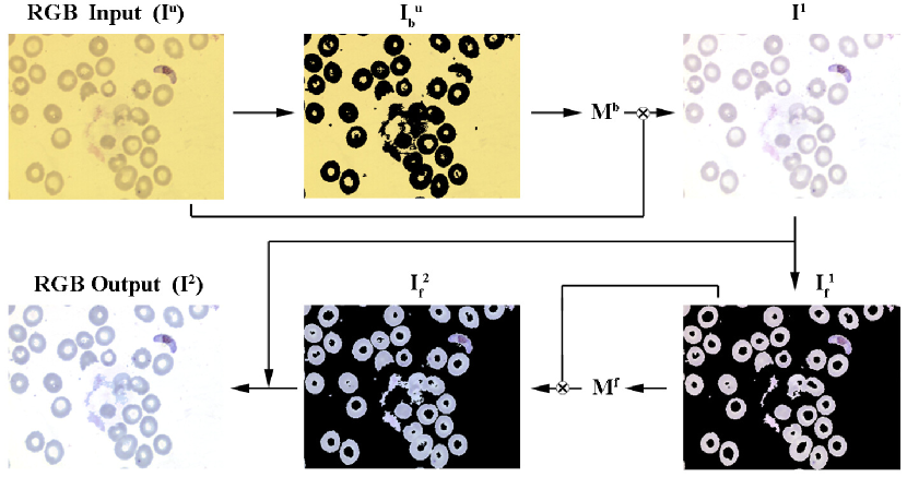
Fig. 1: Color normalization steps: 1) Input RGB image, 2) background pixels are separated, 3) input image is normalized by its background average value (for each channel $RGB$) ($I^{1}$), 4) foreground pixels are extracted $({I_{f}}^{1}_{r,g,b})$, 5) the foreground pixels are normalized $\mathbf{I_{f}}^{2}$, 6) the normalized foreground pixels of each channel are replaced with the ones in $I^{1}$ to obtain output (color corrected image) $I^{2}$.

3 Experimental Results

In order to evaluate the proposed method we have collected 15 images of the same thin blood film (standard Giemsa-stained) field using a Brunel Sp 200 (Brunel, UK) microscope and a Canon A60 digital camera coupled with Unilink (Brunel, UK) adapter. In order to construct the database reference (gray) values, a reference set of 12 thin color film images (of different fields) was prepared; however, the images were not chosen in terms of quality. The only criterion was that the images have to be acquired with the same illumination and camera settings. The illuminant or camera settings were not recorded or required. After an initial normalization with respect to the background channel average values $R,G,B$, the foreground $R,G,B$ channel average values were calculated for each channel ($\mu^{c}_{r}=183,\mu^{c}_{g}=189,\mu^{c}_{b}=214$), respectively, which were then used in the normalizations of the foreground images. To provide a comparison we implemented simple gray world normalization algorithm and also used a MATLAB^TM implementation of Retinex [8]. However, in order to work effectively Retinex implementation [8] requires log-quantized input images, which was not possible to provide with Canon A60. However, we applied pre-normalization with respect to the minimum and maximum channel values. The number of iterations parameter for Retinex was set to 4. To measure and compare the performance, we followed the related works [9, 10] and calculated the RMS (root mean square) of the angular difference:

$$E_{\theta}=acos(\frac{\mathbf{p_{1}}.\mathbf{p_{2}}}{\left\|\mathbf{p_{1}}\right\|\left\|\mathbf{p_{2}}\right\|})$$

where $p_{1}$ and $p_{2}$ are two different output pixel $RGB$ triples.

Fig. 2 shows input images and corresponding outputs from the three different algorithms: database gray world (GW-DB), Retinex, and the proposed (foreground-background separation based) gray world (FG-BG GW). The input images contain significant color casts which result from the different illumination and sensor color balance. In general all three algorithms can remove the color casts in majority of cases, whereas our algorithm can recover colors even in the desaturated image. Figure 3a visualizes the sum of RMS angular differences for each input images, where the RMS difference values for the unprocessed inputs are provided as a reference. It can be seen that the both of Retinex and FG-BG GW algorithms performed best in five images whereas GW-DB, whereas GW performed poor in most of the cases.

Note that, the presented algorithm is not proposed as an iterative process, however it is expected to be idempotent and make no difference if applied to an input image with correct colors. Figure 3b shows the RMS difference between an input-output pair of the FG-BG GW algorithm with respect to consecutive applications. It can be observed the significant difference is obtained in the first run, whereas the algorithm converges rapidly, as the ratios (i.e. diagonal entries of $\mathbf{M}$) approach to $1$. Moreover, we have tested our algorithm on arbitrary thin blood film images of different blood abnormalities from arbitrary internet sources and observed that it provides robust color correction.

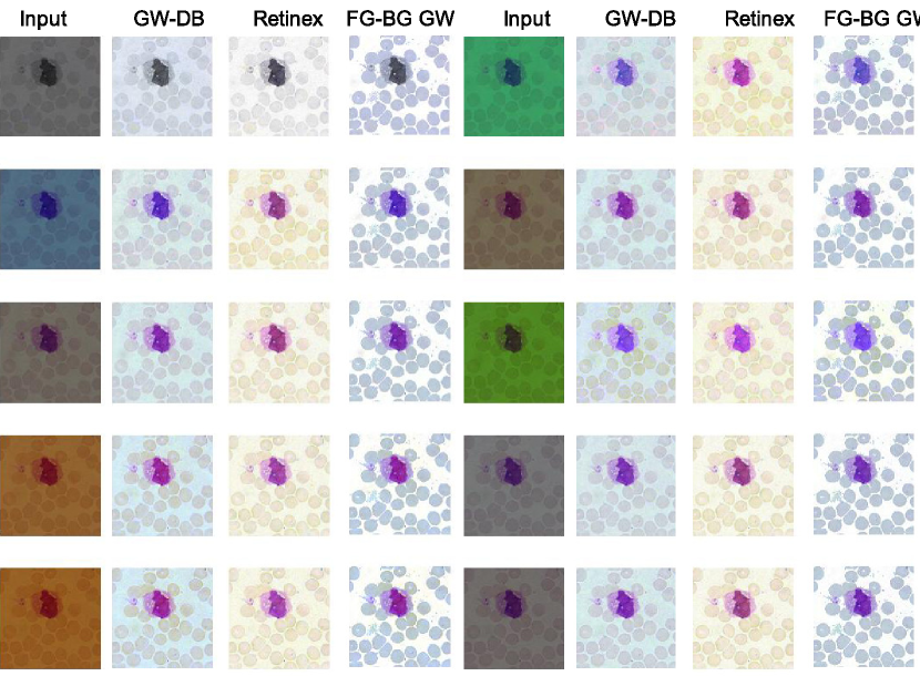
Fig. 2: Different input images of the same field under different imaging conditions and output of gray world (GW), database gray world (GW-DB), Retinex, and proposed gray world algorithm (FG-BG GW).

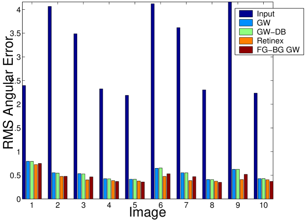
(a)

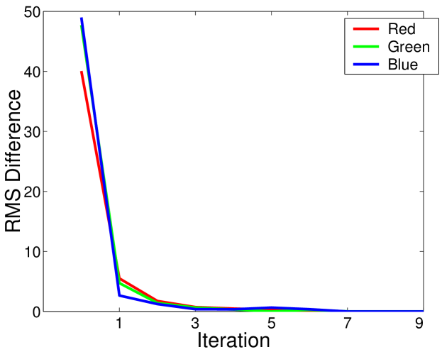
(b)

Fig. 3: (a) Sum of RMS angular differences between color corrected outputs of different algorithms, (b) RMS difference versus iteration of the proposed method for an input and output image.

4 Conclusions

We presented a novel color correction method for peripheral thin blood film images based on the gray world and database gray world assumptions. Our method assumes that plasma (background) is observable in the input image. It further assumes the background is colorless under ideal microscope lighting conditions; it scales the whole image to shift the plasma color towards maximum possible level to reduce the effects of illumination. The foreground color correction assumes that the foreground scene in the image is distributed normally around an average value, which is then scaled to match a value that is calculated from a reference image set of desired color.

We show that it is better than the simple gray world algorithms, whereas it has similar or better performance to Retinex (in terms of RMS angular error). A color correction algorithm must be idempotent if applied to an already normalized image. Our algorithm converges rapidly to a stable state after the first application.

In addition, our algorithm is favorable to Retinex, because the latter requires iterations which are computationally more demanding. However, it is possible to investigate whether the proposed method can be improved with use of Retinex instead of the simple gray world assumption. Moreover, it would be useful to test and compare the performance of the methods in terms of their performance as a preprocessing step to an automatic analysis algorithm.

References

- [1] F. B. Tek, A. G. Dempster, and İzzet Kale, “Parasite detection and identification for automated thin blood film malaria diagnosis,” Computer Vision and Image Understanding, vol. 114, no. 1, pp. 21 – 32, 2010.
- [2] K. Barnard, Practical colour constancy, Ph.d. thesis, Simon Fraser University School of Computing Science, 1999.
- [3] H.-C. Lee, Introduction to Color Imaging Science, Cambridge University Press, UK, 2005.
- [4] C. Grana, G. Pellacani, and S. Seidenari, “Practical color calibration for dermoscopy, applied to a digital epiluminescence microscope,” Skin Research and Technology, vol. 11, pp. 242–247, 2005.
- [5] Y. Yagi and J. R. Gilbertson, “Digital imaging in pathology: the case for standardization,” Journal of Telemedicine and Telecare, vol. 11, pp. 109–116, 2005.
- [6] T. Abe, M. Yamaguchi, Y. Murakami, N. Ohyama, and Y. Yagi, “Color correction of pathological images for different staining-condition slides,” in Proc. 6th International HealthCom Workshop, Odawara, Japan, 2004.
- [7] F. B. Tek, A. G. Dempster, and I. Kale, “A colour normalization method for giemsa-stained blood cell images,” in Proc. Signal Processing and Applications (IEEE), SIU2006, Antalya, Turkey, 2006.
- [8] B. Funt, F. Ciurea, and J. McCann, “Retinex in matlab,” in Proceedings of the IS&T/SID Eighth Color Imaging Conference:Color Science, Systems and Applications, 2000, pp. 112–121.
- [9] S. Hordley and G. Finlayson, “Re-evaluating colour constancy algorithms,” in Proc. of the 17th International Conference on Pattern Recognition, Cambridge, UK, 2004.
- [10] K. Barnard, L. Martin, A. Coath, and B. Funt, “A comparison of computational color constancy algorithms. ii. experiments with image data,” IEEE Transactions on Image Processing, vol. 11, pp. 985–996, 2002.
- [11] K. N. R. M. Rao, Application of Mathematical Morphology to Biomedical Image Processing, Ph.D. thesis, University of Westminster, London, UK, 2004.
- [12] P. Soille, Morphological Image Analysis, Springer-Verlag, Heidelberg, Germany, 2003.