Steady states of elastically-coupled
extensible double-beam systems

Abstract.

Given $\beta\in\mathbb{R}$ and $\varrho,k>0$, we analyze an abstract version of the nonlinear stationary model in dimensionless form

$$\begin{cases}u^{\prime\prime\prime\prime}-\Big{(}\beta+\varrho\int_{0}^{1}|u^{\prime}(s)|^{2}\,{\rm d}s\Big{)}u^{\prime\prime}+k(u-v)=0\\ \vskip 2.27621pt\cr v^{\prime\prime\prime\prime}-\Big{(}\beta+\varrho\int_{0}^{1}|v^{\prime}(s)|^{2}\,{\rm d}s\Big{)}v^{\prime\prime}-k(u-v)=0\end{cases}$$

describing the equilibria of an elastically-coupled extensible double-beam system subject to evenly compressive axial loads. Necessary and sufficient conditions in order to have nontrivial solutions are established, and their explicit closed-form expressions are found. In particular, the solutions are shown to exhibit at most three nonvanishing Fourier modes. In spite of the symmetry of the system, nonsymmetric solutions appear, as well as solutions for which the elastic energy fails to be evenly distributed. Such a feature turns out to be of some relevance in the analysis of the longterm dynamics, for it may lead up to nonsymmetric energy exchanges between the two beams, mimicking the transition from vertical to torsional oscillations.

1. Introduction

1.1. Physical motivations

For engineering purposes, the mathematical modeling process can be viewed as the first step towards the analysis of both static and dynamic responses of actual mechanical structures. Nevertheless, it relies on an idealization of the physical world, and has limits of validity that must be specified. For a given system, different models can be constructed, the “best” being the simplest one able to capture all the essential features needed in the investigation. Among others, models of elastic sandwich-structured composites are experiencing an increasing interest in the literature, mainly due to their wide use in sandwich panels and their applications in many branches of modern civil, mechanical and aerospace engineering [30]. Sandwich structures are in general symmetric, and their variety depends on the configuration of the core. Such devices are designed to have high bending stiffness with overall low density [9, 18]. In particular, sandwich beams, plates and shells are flexible elastic structures built up by attaching two thin and stiff external layers (beams, plates or shells) to a homogeneously-distributed lightweight and thick elastic core [23]. Their interest, which is relevant in structural mechanics, has been recently extended even to nanostructures (see e.g. [6] and references therein).

Models of elastic sandwich structures can be obtained by applying either the Euler-Bernoulli theory for beams or the Kirchhoff-Love theory for thin plates. In this context, several papers have been devoted to the mechanical properties of elastically-connected double Euler-Bernoulli beams systems. For instance, free and forced transverse vibrations of simply supported double-beam systems have been studied in [17, 22, 26], while the articles [31, 32] are concerned with the effect of compressive axial load on free and forced oscillations. Within the framework of nanostructures, axial instability and buckling of double-nanobeam systems have been analyzed in [21, 27].

Once a model is established, the next step is to (possibly) solve the mathematical equations, in order to discover the nature of the system response. In fact, the main goal is to predict and control the actual dynamics. To this end, the analysis of the steady states, and in particular of their closed-form expressions, becomes crucial. This is even more urgent when dealing with nonlinear systems, where the longterm dynamics is strongly influenced by the occurrence of a rich set of stationary solutions.

1.2. The model

In this paper, we aim to classify the stationary solutions, finding their explicit closed-form expressions, to symmetric elastically-coupled extensible double-beam systems. For instance, a sandwich structure composed of two elastic beams bonded to an elastic core (Fig. 1a), or the road bed of a girder bridge composed of an elastic rug connecting two lateral elastic beams (Fig. 1b). In both cases, the mechanical structure can be described by means of two equal beams complying with the nonlinear model of Woinowsky-Krieger [29], which takes into account extensibility, so that large deformations are allowed. The beams are supposed to have the same natural length $\ell>0$, constant mass density, and common thickness $0<h\ll\ell$. At their ends, they are simply supported and subject to evenly distributed axial loads. A system of linear springs models the elastic filler connecting the beams: when the system lies in its natural configuration, the beams are straight and parallel. The distance between the beams is equal to the free lengths of the springs. Denoting by $\nu\in(-1,\tfrac{1}{2})$ the Poisson ratio of the beams, the dynamics of the resulting undamped model is ruled by the following nonlinear equations in dimensionless form (see the final Appendix for more details about the derivation of the model)

(1.1) $$\begin{cases}\displaystyle\frac{\ell(1-\nu)}{h}\Big{(}\partial_{tt}-\frac{h^{2}}{12\ell^{2}}\partial_{ttxx}\Big{)}u+\delta\partial_{xxxx}u-\big{(}\chi+\|\partial_{x}u\|^{2}\big{)}\partial_{xx}u+\kappa(u-v)=0,\\ \vskip 4.83694pt\cr\displaystyle\frac{\ell(1-\nu)}{h}\Big{(}\partial_{tt}-\frac{h^{2}}{12\ell^{2}}\partial_{ttxx}\Big{)}v+\delta\partial_{xxxx}v-\big{(}\chi+\|\partial_{x}v\|^{2}\big{)}\partial_{xx}v-\kappa(u-v)=0,\end{cases}$$

having set

$$\|f\|=\bigg{(}\int_{0}^{1}|f(s)|^{2}\,{\rm d}s\bigg{)}^{\frac{1}{2}}.$$

In the vertical plane ($x$-$z$), system (1.1) describes the in-plane downward rescaled deflections of the midline of the beams

$$u,v:[0,1]\times\mathbb{R}^{+}\to\mathbb{R}$$

with respect to their natural configuration (see Fig. 1a). It may be also used to describe out-of-plane rescaled deflections of the same double-beam structure, accounting for both vertical and torsional oscillations (see Fig. 1b). In the latter situation, each beam is assumed to swing in a vertical plane and the lateral movements are neglected. The structural constants $\delta,\kappa>0$ are related to the common flexural rigidity of the beams and the common stiffness of the inner elastic springs, respectively, whereas the parameter $\chi\in\mathbb{R}$ summarizes the effect of the axial force acting at the right ends of the beams: positive when the beams are stretched, negative when compressed.

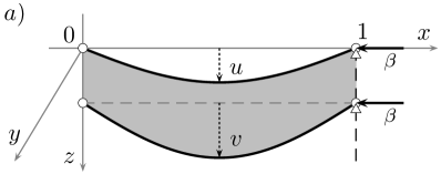
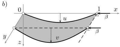
Figure 1. In-plane (a) and out-of-plane (b) deflections of a double-beam system under compressive axial loads $\beta={\chi}/{\delta}.$

In this work, we are interested in the stationary solutions to the evolutionary problem (1.1), subject to the hinged boundary conditions. Namely, setting

$$\beta=\frac{\chi}{\delta}\in\mathbb{R},\qquad\varrho=\frac{1}{\delta}>0,\qquad k=\frac{\kappa}{\delta}>0,$$

we consider the dimensionless system of ODEs

(1.2) $$\begin{cases}u^{\prime\prime\prime\prime}-\big{(}\beta+\varrho\|u^{\prime}\|^{2}\big{)}u^{\prime\prime}+k(u-v)=0,\\ \vskip 2.84526pt\cr v^{\prime\prime\prime\prime}-\big{(}\beta+\varrho\|v^{\prime}\|^{2}\big{)}v^{\prime\prime}-k(u-v)=0,\end{cases}$$

supplemented with the boundary conditions

(1.3) $$\begin{cases}u(0)=u(1)=u^{\prime\prime}(0)=u^{\prime\prime}(1)=0,\\ \vskip 1.42262pt\cr v(0)=v(1)=v^{\prime\prime}(0)=v^{\prime\prime}(1)=0.\end{cases}$$

It is apparent that problem (1.2)-(1.3) always admits the trivial solution $u=v=0$, while the occurrence and the complexity of nontrivial solutions strongly depend on the values of structural dimensionless parameters $\beta,\varrho,k$, all of which are allowed to be large (see the final comment in the Appendix).

1.3. Earlier results on single-beam equations

When system (1.2) is uncoupled (i.e. in the limit situation when $k=0$), the analysis reduces to the one of the single Woinowsky-Krieger beam

$$u^{\prime\prime\prime\prime}-\big{(}\beta+\varrho\|u^{\prime}\|^{2}\big{)}u^{\prime\prime}=0.$$

In this case, it is well-known that an increasing compressive axial load leads to a series of fork bifurcations. The critical values of $\beta$ at which bifurcations occur depend on the eigenvalues of the differential operator (see e.g. [2, 8]). After exceeding these values, the axial compression is sustained in one of two states of equilibrium: a purely compressed state with no lateral deviation (the trivial solution) or two symmetric laterally-deformed configurations (buckled solutions). This is why the phenomenon is usually referred to as buckling. Another interesting model, formally obtained by neglecting the second equation of system (1.2) and by taking $v\equiv 0$ in the first one, reads

$$u^{\prime\prime\prime\prime}-\big{(}\beta+\varrho\|u^{\prime}\|^{2}\big{)}u^{\prime\prime}+ku=0,$$

namely, a single Woinowsky-Krieger beam which relies on an elastic foundation. In this case, bifurcations of the trivial solution split into two series, whose critical values depend also on the ratio $k$ between the parameters $\kappa$ and $\delta$ connected with the stiffness of the foundation and the flexural rigidity of the beam [3].

1.4. The goal of the present work

Clearly, when the double-beam system (1.2) is considered, the picture becomes much more difficult. To the best of our knowledge, in spite of the quite large number of papers about statics and dynamics of single Woinowsky-Krieger beams (e.g. [2, 3, 7, 8, 10, 11, 12, 14, 15, 24]), no analytic results concerning models with a coupling between two (or more) nonlinear beams of this type are available in the literature. This may be due to the fact that classifying and finding closed-form expressions for the solutions to equations of this kind is in general a very difficult, if not impossible, task. Indeed, it is usually unavoidable to replace distributed characteristics with discrete ones, so producing approximate solutions by resorting to some discretization procedures. Unfortunately, this strategy can be hardly applied when multiple stable states occur (see e.g. [18] and references therein).

Here, our aim is to fill this gap. To this end, we first recast (1.2)-(1.3) into an abstract nonlinear system involving an arbitrary strictly positive selfadjoint linear operator $A$ with compact inverse. Then, we classify all the nontrivial solutions, finding also their explicit expressions. In particular, every solution is shown to exhibit at most three nonvanishing Fourier modes. According to our classification, the set of stationary solutions to nonlinear double-beam systems is very rich. The nonlinear terms accounting for extensibility substantially influence the instability (or buckling): the effects are higher with increasing values of (minus) the axial-load parameter $\beta$, and give rise to both in-phase (synchronous) buckling modes and out-of-phase (asynchronous) buckling modes. This feature becomes quite important in the study of the longterm behavior, as it may lead up to nonsymmetric energy exchanges between the two beams under small perturbations. In the asymptotic dynamics of a double-beam structure like the road bed of a girder bridge (Fig. 1b), a nonsymmetric energy exchange of this kind is apt to mimic the transition from vertical to torsional oscillations, such as those occurred in the collapse of the Tacoma Narrows suspension bridge (see e.g. [20] and references therein). Another remarkable fact is that the model (1.2) has been derived under the assumption that the ratio $h/\ell$ between the thickness and the natural length of the beam is very small; the critical values at which bifurcations occur are consistent with such an assumption, namely, they are of order $h/\ell$ as well. We also stress that system (1.2) is dimensionless, and no physical parameters have been artificially set equal to one. Finally it is worth noting that, as a consequence of the abstract formulation, all the results are valid also for multidimensional structures. In particular, they are applicable to flexible double-plate sandwich structures with hinged boundaries, provided that the plates are modeled according to the Berger’s approach [1, 16].

1.5. Plan of the paper

In the next §2 we introduce the aforementioned operator $A$, and we rewrite (1.2)-(1.3) in an abstract form. In §3 we prove that every solution can be expressed as a linear combination of at most three distinct eigenvectors of $A$. The subsequent §4 deals with the analysis of unimodal solutions (i.e. solutions with only one eigenvector involved). In particular, we show that not only a double series of fork bifurcations of the trivial solution occur, but also buckled solutions may suffer from a further bifurcation when $-\beta$ exceeds some greater critical value. In §5 we study the so-called equidistributed energy solutions (i.e. solutions with evenly distributed elastic energy), and we prove that bimodal and trimodal steady states pop up. In §6 we classify the general (not necessarily equidistributed) bimodal solutions, while in §7 we show that every trimodal solution is necessarily an equidistributed energy solution, The final §8 is devoted to a comparison with some single-beam equations previously studied in the literature. The derivation of the evolutionary physical model (1.1) is carried out in full detail in the concluding Appendix.

2. The Abstract Model

Let $({\rm H},\langle\cdot,\cdot\rangle,\|\cdot\|)$ be a separable real Hilbert space, and let

$$A:{\mathfrak{D}}(A)\Subset{\rm H}\to{\rm H}$$

be a strictly positive selfadjoint linear operator, where the (dense) embedding ${\mathfrak{D}}(A)\Subset{\rm H}$ is compact. In particular, the inverse $A^{-1}$ of $A$ turns out to be a compact operator on ${\rm H}$. Accordingly, for $r\geq 0$, we introduce the compactly nested family of Hilbert spaces (the index $r$ will be omitted whenever zero)

$${\rm H}^{r}={\mathfrak{D}}(A^{\frac{r}{2}}),\qquad\langle u,v\rangle_{r}=\langle A^{\frac{r}{2}}u,A^{\frac{r}{2}}v\rangle,\qquad\|u\|_{r}=\|A^{\frac{r}{2}}u\|.$$

Then, given $\beta\in\mathbb{R}$ and $\varrho,k>0$, we consider the abstract nonlinear stationary problem in the unknown variables $(u,v)\in{\rm H}^{2}\times{\rm H}^{2}$

(2.1) $$\begin{cases}A^{2}u+C_{u}Au+k(u-v)=0,\\ \vskip 1.99168pt\cr A^{2}v+C_{v}Av-k(u-v)=0,\end{cases}$$

where

(2.2) $$C_{u}=\beta+\varrho\|u\|_{1}^{2}C_{v}=\beta+\varrho\|v\|_{1}^{2}.$$

Definition 2.1.

A couple $(u,v)\in{\rm H}^{2}\times{\rm H}^{2}$ is called a weak solution to (2.1) if

(2.3) $$\begin{cases}\langle u,\phi\rangle_{2}+C_{u}\langle u,\phi\rangle_{1}+k\langle(u-v),\phi\rangle=0,\\ \vskip 1.99168pt\cr\langle v,\psi\rangle_{2}+C_{v}\langle v,\psi\rangle_{1}-k\langle(u-v),\psi\rangle=0,\end{cases}$$

for every test $(\phi,\psi)\in{\rm H}^{2}\times{\rm H}^{2}$.

It is apparent that the trivial solution $u=v=0$ always exists.

Example 2.2.

The concrete physical system (1.2) is recovered by setting ${\rm H}=L^{2}(0,1)$ and $A=L$, where

$$L=-\frac{{\rm d}^{2}}{{\rm d}x^{2}}\qquad\text{with}\qquad{\mathfrak{D}}(L)=H^{2}(0,1)\cap H_{0}^{1}(0,1).$$

Here $L^{2}(0,1)$, as well as $H_{0}^{1}(0,1)$ and $H^{2}(0,1)$, denote the usual Lebesgue and Sobolev spaces on the unit interval $(0,1)$. In particular

$${\rm H}^{2}=H^{2}(0,1)\cap H_{0}^{1}(0,1)\,\,\,\Subset\,\,\,{\rm H}^{1}=H_{0}^{1}(0,1)\,\,\,\Subset\,\,\,{\rm H}=L^{2}(0,1).$$

Notation. For any $n\in\mathbb{N}=\{1,2,3,\ldots\}$ we denote by

$$0<\lambda_{n}\to\infty$$

the increasing sequence of eigenvalues of $A$, and by $e_{n}\in{\rm H}$ the corresponding normalized eigenvectors, which form a complete orthonormal basis of ${\rm H}$. In this work, all the eigenvalues $\lambda_{n}$ are assumed to be simple, which is certainly true for the concrete realization $A=L$ arising in the considered physical models. Indeed, in such a case, the eigenvalues are equal to

$$\lambda_{n}=n^{2}\pi^{2}$$

with corresponding eigenvectors

$$e_{n}(x)=\sqrt{2}\sin{(n\pi x)}.$$

3. General Structure of the Solutions

In this section we provide two general results on the solutions to system (2.1). To this end, we introduce the set of effective modes

$$\mathbb{E}=\{n:\lambda_{n}<-\beta\}.$$

Clearly,

(3.1) $$\mathbb{E}\not=\emptyset\quad\Leftrightarrow\quad\beta<-\lambda_{1}.$$

Therefore, if $\mathbb{E}\neq\emptyset$,

$$\mathbb{E}=\{1,2,\ldots,n_{\star}\},$$

where

$$n_{\star}=\max\{n:\lambda_{n}<-\beta\}=|\mathbb{E}|.$$

Example 3.1.

When $A=L$ (the Laplace-Dirichlet operator introduced in the previous section), we have

$$\mathbb{E}=\big{\{}n:n^{2}\pi^{2}<-\beta\big{\}}.$$

Accordingly, in the nontrivial case $\beta<0$,

$$|\mathbb{E}|=\left\lceil\sqrt{-\frac{\beta}{\pi^{2}}}\,\,\right\rceil-1,$$

the symbol $\lceil a\rceil$ standing for the smallest integer greater than or equal to $a$.

We begin to prove that the picture is trivial whenever the set $\mathbb{E}$ is empty.

Proposition 3.2.

If $\mathbb{E}=\emptyset$ system (2.1) admits only the trivial solution.

Proof.

Let $(u,v)$ be a weak solution to (2.1). Choosing $(\phi,\psi)=(u,v)$ in the weak formulation (2.3), and adding the resulting expressions, we obtain the identity

$$\|u\|_{2}^{2}+\|v\|_{2}^{2}+(\beta+\varrho\|u\|_{1}^{2})\|u\|_{1}^{2}+(\beta+\varrho\|v\|_{1}^{2})\|v\|_{1}^{2}+k\|u-v\|^{2}=0.$$

Then, exploiting the Poincaré inequality

$$\lambda_{1}\|w\|_{1}^{2}\leq\|w\|_{2}^{2},\quad\forall w\in{\rm H}^{2},$$

we infer that

$$(\lambda_{1}+\beta)(\|u\|_{1}^{2}+\|v\|_{1}^{2})+\varrho\|u\|_{1}^{4}+\varrho\|v\|_{1}^{4}+k\|u-v\|^{2}\leq 0,$$

and, since $\lambda_{1}+\beta\geq 0$, we conclude that $u=v=0$. ∎

Accordingly, from now on we will assume (often without explicit mention) that (3.1) be satisfied. As it will be clear from the subsequent analysis, this condition turns out to be sufficient as well in order to have nontrivial solutions. Hence, a posteriori, we can reformulate Proposition 3.2 by saying that system (2.1) admits nontrivial solutions if and only if the set $\mathbb{E}$ is nonempty.

The next result shows that every weak solution can be written as linear combination of at most three distinct eigenvectors of $A$.

Lemma 3.3.

Let $(u,v)$ be a weak solution of system (2.1). Then

$$u=\sum_{n}\alpha_{n}e_{n}v=\sum_{n}\gamma_{n}e_{n}$$

for some $\alpha_{n},\gamma_{n}\in\mathbb{R}$, where $\alpha_{n}\not=0$ for at most three distinct values of $n\in\mathbb{N}$. Moreover,

$$\alpha_{n}=0\quad\Leftrightarrow\quad\gamma_{n}=0.$$

Proof.

Let $(u,v)$ be a weak solution to (2.1). Then, writing

$$u=\sum_{n}\alpha_{n}e_{n}v=\sum_{n}\gamma_{n}e_{n}$$

for some $\alpha_{n},\gamma_{n}\in\mathbb{R}$, and choosing $\phi=\psi=e_{n}$ in the weak formulation (2.3), we obtain for every $n\in\mathbb{N}$ the system

(3.2) $$\begin{cases}\lambda_{n}^{2}\alpha_{n}+C_{u}\lambda_{n}\alpha_{n}+k(\alpha_{n}-\gamma_{n})=0,\\ \lambda_{n}^{2}\gamma_{n}+C_{v}\lambda_{n}\gamma_{n}-k(\alpha_{n}-\gamma_{n})=0.\end{cases}$$

It is apparent that

$$\alpha_{n}=0\quad\Leftrightarrow\quad\gamma_{n}=0.$$

Substituting the first equation into the second one, we get

$$\gamma_{n}(\lambda_{n}^{2}+C_{v}\lambda_{n}+k)(\lambda_{n}^{2}+C_{u}\lambda_{n}+k)=k^{2}\gamma_{n}.$$

Hence, if $\gamma_{n}\not=0$ (and so $\alpha_{n}\not=0$), we end up with

$$\lambda_{n}^{3}+(C_{u}+C_{v})\lambda_{n}^{2}+(C_{u}C_{v}+2k)\lambda_{n}+k(C_{u}+C_{v})=0.$$

Since the equation above admits at most three distinct solutions $\lambda_{n_{i}}$ we are done. ∎

Summarizing, every weak solution $(u,v)$ can be written as

(3.3) $$u=\sum_{i=1}^{3}\alpha_{n_{i}}e_{n_{i}}v=\sum_{i=1}^{3}\gamma_{n_{i}}e_{n_{i}},$$

for three distinct $n_{i}\in\mathbb{N}$ and some coefficients $\alpha_{n}{{}_{i}},\gamma_{n_{i}}\in\mathbb{R}$. In particular, from (2.2), we deduce the explicit expressions

(3.4) $$C_{u}=\beta+\varrho\sum_{i=1}^{3}\lambda_{n_{i}}\alpha_{n_{i}}^{2}C_{v}=\beta+\varrho\sum_{i=1}^{3}\lambda_{n_{i}}\gamma_{n_{i}}^{2}.$$

In addition, when

$$\alpha_{n_{i}}\not=0\quad\Leftrightarrow\quad\gamma_{n_{i}}\not=0,$$

the corresponding eigenvalue $\lambda_{n_{i}}$ is a root of the cubic polynomial

$$P(\lambda)=\lambda^{3}+(C_{u}+C_{v})\lambda^{2}+(C_{u}C_{v}+2k)\lambda+k(C_{u}+C_{v}).$$

Notably, when the equality $C_{u}=C_{v}$ holds, the polynomial $P(\lambda)$ can be written in the simpler form

$$P(\lambda)=(\lambda+C_{u})(\lambda^{2}+C_{u}\lambda+2k).$$

Remark 3.4.

Adding the two equations of system (3.2), we infer that

(3.5) $$\lambda_{n}=-\frac{C_{u}\alpha_{n}+C_{v}\gamma_{n}}{\alpha_{n}+\gamma_{n}}$$

whenever $\alpha_{n}+\gamma_{n}\not=0$. This relation will be crucial for our purposes.

As an immediate consequence of Lemma 3.3, we also have

Corollary 3.5.

Every weak solution $(u,v)$ is actually a strong solution. Namely, $(u,v)\in{\rm H}^{4}\times{\rm H}^{4}$ and (2.1) holds. Even more so, $(u,v)\in{\rm H}^{r}\times{\rm H}^{r}$ for every $r$.

Remark 3.6.

In the concrete situation when $A=L$, every weak solution $(u,v)$ is regular, that is, $(u,v)\in\mathcal{C}^{\infty}([0,1])\times\mathcal{C}^{\infty}([0,1])$.

Finally, in the light of Lemma 3.3, we give the following definition.

Definition 3.7.

We call a solution $(u,v)$ unimodal, bimodal or trimodal if it involves one, two or three distinct eigenvectors, that is, if $\alpha_{n}\not=0$ (and so $\gamma_{n}\not=0$) for one, two or three indexes $n$, respectively.

4. Unimodal Solutions

We now focus on unimodal solutions. More precisely, we look for solutions $(u,v)$ of the form

(4.1) $$\begin{cases}u=\alpha_{n}e_{n},\\ v=\gamma_{n}e_{n},\end{cases}$$

for a fixed $n\in\mathbb{N}$ and some coefficients $\alpha_{n},\gamma_{n}\not=0$. In order to classify such solutions, we introduce the positive sequences

$$\mu_{n}=\frac{2k}{\lambda_{n}}+\lambda_{n}\nu_{n}=\frac{3k}{\lambda_{n}}+\lambda_{n},$$

along with the (disjoint) subsets of $\mathbb{E}$

$$\mathbb{E}_{1}=\{n:\lambda_{n}<-\beta\leq\mu_{n}\},$$

$$\mathbb{E}_{2}=\{n:\mu_{n}<-\beta\leq\nu_{n}\},$$

$$\mathbb{E}_{3}=\{n:\nu_{n}<-\beta\}.$$

Clearly,

$$\mathbb{E}_{1}\cup\mathbb{E}_{2}\cup\mathbb{E}_{3}=\mathbb{E}.$$

Then, we consider the real numbers (whenever defined)

(4.2) $$\begin{cases}\displaystyle\alpha_{n,1}^{\pm}=\pm\sqrt{\frac{-\beta-\lambda_{n}}{\varrho{\lambda_{n}}}},\\ \vskip 2.84526pt\cr\displaystyle\alpha_{n,2}^{\pm}=\pm\sqrt{\frac{-\beta-\mu_{n}}{\varrho{\lambda_{n}}}},\\ \vskip 2.84526pt\cr\displaystyle\alpha_{n,3}^{\pm}=\pm\sqrt{\frac{-\beta+\mu_{n}-\nu_{n}-\lambda_{n}+\sqrt{(\beta+\lambda_{n}+\mu_{n}-\nu_{n})(\beta+\nu_{n})}}{2\varrho\lambda_{n}}},\\ \vskip 2.84526pt\cr\displaystyle\alpha_{n,4}^{\pm}=\pm\sqrt{\frac{-\beta+\mu_{n}-\nu_{n}-\lambda_{n}-\sqrt{(\beta+\lambda_{n}+\mu_{n}-\nu_{n})(\beta+\nu_{n})}}{2\varrho\lambda_{n}}},\end{cases}$$

hereafter called unimodal amplitudes, or u-amplitudes for brevity. By elementary calculations, one can easily verify that

$$\alpha_{n,1}^{\pm}\in\mathbb{R}\quad\Leftrightarrow\quad\lambda_{n}\leq-\beta,$$

$$\alpha_{n,2}^{\pm}\in\mathbb{R}\quad\Leftrightarrow\quad\mu_{n}\leq-\beta,$$

$$\alpha_{n,3}^{\pm}\in\mathbb{R}\quad\Leftrightarrow\quad\nu_{n}\leq-\beta,$$

$$\alpha_{n,4}^{\pm}\in\mathbb{R}\quad\Leftrightarrow\quad\nu_{n}\leq-\beta.$$

Lemma 4.1.

For every fixed $n\in\mathbb{N}$, let us consider the set

$$\Gamma_{n}=\{\alpha_{n,i}^{\pm}:i=1,2,3,4\}.$$

Then, $\Gamma_{n}$ contains exactly

• 2 distinct nontrivial u-amplitudes $\{\alpha_{n,1}^{\pm}\}$ if $n\in\mathbb{E}_{1}$;

• 4 distinct nontrivial u-amplitudes $\{\alpha_{n,1}^{\pm},\alpha_{n,2}^{\pm}\}$ if $n\in\mathbb{E}_{2}$;

• 8 distinct nontrivial u-amplitudes $\{\alpha_{n,1}^{\pm},\alpha_{n,2}^{\pm},\alpha_{n,3}^{\pm},\alpha_{n,4}^{\pm}\}$ if $n\in\mathbb{E}_{3}$.

If $n\notin\mathbb{E}$, the set $\Gamma_{n}$ is either empty or it contains exactly the (trivial) u-amplitudes $\alpha_{n,1}^{+}=\alpha_{n,1}^{-}=0$.

Proof.

We analyze separately all the possible cases.

• If $n\in\mathbb{E}_{1}$, there are only two distinct nontrivial u-amplitudes, that is, $\alpha_{n,1}^{\pm}$. Indeed, when $\mu_{n}=-\beta$,

  $$\alpha_{n,2}^{\pm}=0.$$

• If $n\in\mathbb{E}_{2}$, there are only four distinct nontrivial u-amplitudes, that is, $\alpha_{n,1}^{\pm}$ and $\alpha_{n,2}^{\pm}$. Indeed, when $\nu_{n}=-\beta$,

  $$\alpha_{n,3}^{+}=\alpha_{n,4}^{+}=\alpha_{n,2}^{+}\alpha_{n,3}^{-}=\alpha_{n,4}^{-}=\alpha_{n,2}^{-}.$$

• If $n\in\mathbb{E}_{3}$, all the eight u-amplitudes $\alpha_{n,i}^{\pm}$ are distinct and nontrivial.

If $n\notin\mathbb{E}$, all the u-amplitudes $\alpha_{n,i}^{\pm}$, whenever defined, are trivial. In particular, the only two allowed amplitudes are $\alpha_{n,1}^{+}=\alpha_{n,1}^{-}=0$. ∎

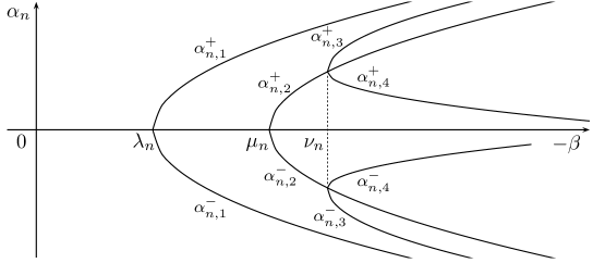
Figure 2. The u-amplitudes $\alpha_{n,i}^{\pm}$ for a fixed $n\in\mathbb{N}$.

We are now in a position to state our main result on unimodal solutions.

Theorem 4.2.

System (2.1) admits nontrivial unimodal solutions if and only if the set $\mathbb{E}$ is nonempty. More precisely, for every $n\in\mathbb{N}$, one of the following disjoint situations occurs.

• If $n\in\mathbb{E}_{1}$, we have exactly 2 nontrivial unimodal solutions of the form

  $$(u,v)=\begin{cases}(\alpha_{n,1}^{+}\,e_{n},\,\alpha_{n,1}^{+}\,e_{n})\\ (\alpha_{n,1}^{-}\,e_{n},\,\alpha_{n,1}^{-}\,e_{n}).\end{cases}$$

• If $n\in\mathbb{E}_{2}$, we have exactly 4 nontrivial unimodal solutions of the form

  $$(u,v)=\begin{cases}(\alpha_{n,1}^{+}\,e_{n},\,\alpha_{n,1}^{+}\,e_{n})\\ (\alpha_{n,1}^{-}\,e_{n},\,\alpha_{n,1}^{-}\,e_{n})\\ (\alpha_{n,2}^{+}\,e_{n},\,\alpha_{n,2}^{-}\,e_{n})\\ (\alpha_{n,2}^{-}\,e_{n},\,\alpha_{n,2}^{+}\,e_{n}).\end{cases}$$

• If $n\in\mathbb{E}_{3}$, we have exactly 8 nontrivial unimodal solutions of the form

  $$(u,v)=\begin{cases}(\alpha_{n,1}^{+}\,e_{n},\,\alpha_{n,1}^{+}\,e_{n})\\ (\alpha_{n,1}^{-}\,e_{n},\,\alpha_{n,1}^{-}\,e_{n})\\ (\alpha_{n,2}^{+}\,e_{n},\,\alpha_{n,2}^{-}\,e_{n})\\ (\alpha_{n,2}^{-}\,e_{n},\,\alpha_{n,2}^{+}\,e_{n})\\ (\alpha_{n,3}^{+}\,e_{n},\,\alpha_{n,4}^{-}\,e_{n})\\ (\alpha_{n,3}^{-}\,e_{n},\,\alpha_{n,4}^{+}\,e_{n})\\ (\alpha_{n,4}^{+}\,e_{n},\,\alpha_{n,3}^{-}\,e_{n})\\ (\alpha_{n,4}^{-}\,e_{n},\,\alpha_{n,3}^{+}\,e_{n}).\end{cases}$$

• If $n\notin\mathbb{E}$, all the unimodal solutions involving the eigenvector $e_{n}$ are trivial.

In summary, system (2.1) admits $2|\mathbb{E}_{1}|+4|\mathbb{E}_{2}|+8|\mathbb{E}_{3}|$ nontrivial unimodal solutions.

Proof.

Let us look for nontrivial solutions $(u,v)$ of the form (4.1). Choosing $\phi=\psi=e_{n}$ in the weak formulation (2.3) and recalling (3.4), we obtain the system

$$\begin{cases}\lambda_{n}^{2}\alpha_{n}+(\beta+\varrho\lambda_{n}\alpha_{n}^{2})\lambda_{n}\alpha_{n}+k(\alpha_{n}-\gamma_{n})=0,\\ \vskip 0.85358pt\cr\lambda_{n}^{2}\gamma_{n}+(\beta+\varrho\lambda_{n}\gamma_{n}^{2})\lambda_{n}\gamma_{n}-k(\alpha_{n}-\gamma_{n})=0,\end{cases}$$

which, setting

$$\eta_{n}=1+\frac{\beta}{\lambda_{n}}+\frac{k}{\lambda_{n}^{2}}\omega_{n}=\frac{\lambda_{n}^{2}}{k},$$

can be rewritten as

(4.3) $$\begin{cases}\gamma_{n}=\omega_{n}\alpha_{n}(\eta_{n}+\varrho\alpha_{n}^{2}),\\ \alpha_{n}=\omega_{n}\gamma_{n}(\eta_{n}+\varrho\gamma_{n}^{2}).\end{cases}$$

Solving with respect to $\alpha_{n}$, we arrive at the nine-order equation

$$\alpha_{n}(\varrho^{4}\alpha_{n}^{8}\omega_{n}^{4}+3\varrho^{3}\alpha_{n}^{6}\omega_{n}^{4}\eta_{n}+3\varrho^{2}\alpha_{n}^{4}\omega_{n}^{4}\eta_{n}^{2}+\varrho\alpha_{n}^{2}\omega_{n}^{4}\eta_{n}^{3}+\varrho\alpha_{n}^{2}\omega_{n}^{2}\eta_{n}+\omega_{n}^{2}\eta_{n}^{2}-1)=0.$$

If $\alpha_{n}=0$ the solution is trivial (since in this case also $\gamma_{n}$ is zero). Otherwise, introducing the auxiliary variable

$$x_{n}=\omega_{n}(\eta_{n}+\varrho\alpha_{n}^{2}),$$

we end up with

$$(x_{n}^{2}-1)(x_{n}^{2}-x_{n}\omega_{n}\eta_{n}+1)=0.$$

Making use of the relations

(4.4) $$\begin{cases}\displaystyle\omega_{n}\eta_{n}=-\frac{\lambda_{n}}{k}\big{(}-\beta+\mu_{n}-\nu_{n}-\lambda_{n}\big{)},\\ \vskip 4.2679pt\cr\displaystyle\omega_{n}^{2}\eta_{n}^{2}-4=\frac{\lambda_{n}^{2}}{k^{2}}\big{(}\beta+\lambda_{n}+\mu_{n}-\nu_{n}\big{)}(\beta+\nu_{n}),\end{cases}$$

one can easily realize that the solutions are the u-amplitudes $\alpha_{n,i}^{\pm}$ given by (4.2). Hence, according to Lemma 4.1, we have exactly

• 2 distinct nontrivial solutions $\{\alpha_{n,1}^{\pm}\}$ for every $n\in\mathbb{E}_{1}$;

• 4 distinct nontrivial solutions $\{\alpha_{n,1}^{\pm},\alpha_{n,2}^{\pm}\}$ for every $n\in\mathbb{E}_{2}$;

• 8 distinct nontrivial solutions $\{\alpha_{n,1}^{\pm},\alpha_{n,2}^{\pm},\alpha_{n,3}^{\pm},\alpha_{n,4}^{\pm}\}$ for every $n\in\mathbb{E}_{3}$.

By the same token, when $n\notin\mathbb{E}$, we have only the trivial solution. We are left to find the explicit values $\gamma_{n,i}^{\pm}$, which can be obtained from (4.3). To this end, it is apparent to see that

$$\begin{cases}\gamma_{n,1}^{\pm}=\alpha_{n,1}^{\pm},\\ \vskip 2.84526pt\cr\gamma_{n,2}^{\pm}=\alpha_{n,2}^{\mp}.\end{cases}$$

Moreover, invoking (4.4) and observing that the product $\omega_{n}\eta_{n}$ is negative when $n\in\mathbb{E}_{3}$,

$$\gamma_{n,3}^{\pm} =\pm\frac{\sqrt{k}\big{(}\omega_{n}\eta_{n}+\sqrt{\omega_{n}^{2}\eta_{n}^{2}-4}\big{)}}{2}\sqrt{\frac{-\omega_{n}\eta_{n}+\sqrt{\omega_{n}^{2}\eta_{n}^{2}-4}}{2\varrho\lambda_{n}^{2}}}$$

$$=\mp\sqrt{k}\sqrt{\frac{-\omega_{n}\eta_{n}-\sqrt{\omega_{n}^{2}\eta_{n}^{2}-4}}{2\varrho\lambda_{n}^{2}}}=\alpha_{n,4}^{\mp},$$

and

$$\gamma_{n,4}^{\pm}= =\pm\frac{\sqrt{k}\big{(}\omega_{n}\eta_{n}-\sqrt{\omega_{n}^{2}\eta_{n}^{2}-4}\big{)}}{2}\sqrt{\frac{-\omega_{n}\eta_{n}-\sqrt{\omega_{n}^{2}\eta_{n}^{2}-4}}{2\varrho\lambda_{n}^{2}}}$$

$$=\mp\sqrt{k}\sqrt{\frac{-\omega_{n}\eta_{n}+\sqrt{\omega_{n}^{2}\eta_{n}^{2}-4}}{2\varrho\lambda_{n}^{2}}}=\alpha_{n,3}^{\mp}.$$

The theorem is proved. ∎

5. Equidistributed Energy Solutions

In order to investigate the existence of solutions to system (2.1) which are not necessarily unimodal, we begin to analyze a particular but still very interesting situation.

Definition 5.1.

A nontrivial solution $(u,v)$ is called an equidistributed energy solution (ee-solution for brevity) if

(5.1) $$\|u\|_{1}=\|v\|_{1}\quad\Leftrightarrow\quad C_{u}=C_{v}.$$

At first glance, this condition might look restrictive. Though, as we will see in the next two lemmas, ee-solutions are in fact quite general. In particular, they pop up whenever a mode of $u$ is equal or opposite to the corresponding mode of $v$.

Lemma 5.2.

With reference to (3.3), if

$$\alpha_{n_{i}}\alpha_{n_{j}}=\pm\gamma_{n_{i}}\gamma_{n_{j}}\not=0$$

for some (possibly coinciding) $n_{i},n_{j}$, then $(u,v)$ is an ee-solution. In particular, this is the case when

$$|\alpha_{n_{i}}|=|\gamma_{n_{i}}|\not=0$$

for some $n_{i}$.

Proof.

Let $n_{i},n_{j}$ be such that

$$\alpha_{n_{i}}\alpha_{n_{j}}=\pm\gamma_{n_{i}}\gamma_{n_{j}}\not=0.$$

Choosing $\phi=\psi=e_{n_{i}}$ in the weak formulation (2.3), we obtain

(5.2) $$\begin{cases}\lambda_{n_{i}}^{2}\alpha_{n_{i}}+C_{u}\lambda_{n_{i}}\alpha_{n_{i}}+k(\alpha_{n_{i}}-\gamma_{n_{i}})=0,\\ \lambda_{n_{i}}^{2}\gamma_{n_{i}}+C_{v}\lambda_{n_{i}}\gamma_{n_{i}}-k(\alpha_{n_{i}}-\gamma_{n_{i}})=0,\end{cases}$$

while, choosing $\phi=\psi=e_{n_{j}}$, we get

(5.3) $$\begin{cases}\lambda_{n_{j}}^{2}\alpha_{n_{j}}+C_{u}\lambda_{n_{j}}\alpha_{n_{j}}+k(\alpha_{n_{j}}-\gamma_{n_{j}})=0,\\ \lambda_{n_{j}}^{2}\gamma_{n_{j}}+C_{v}\lambda_{n_{j}}\gamma_{n_{j}}-k(\alpha_{n_{j}}-\gamma_{n_{j}})=0.\end{cases}$$

Then, from (5.2),

$$\begin{cases}\displaystyle C_{u}=-\lambda_{n_{i}}-\frac{k(\alpha_{n_{i}}-\gamma_{n_{i}})}{\lambda_{n_{i}}\alpha_{n_{i}}},\\ \vskip 3.1298pt\cr\displaystyle C_{v}=-\lambda_{n_{i}}+\frac{k(\alpha_{n_{i}}-\gamma_{n_{i}})}{\lambda_{n_{i}}\gamma_{n_{i}}}.\end{cases}$$

These expressions, substituted into (5.3), yield

$$\begin{cases}\lambda_{n_{j}}^{2}\lambda_{n_{i}}\alpha_{n_{i}}\alpha_{n_{j}}-\lambda_{n_{i}}^{2}\lambda_{n_{j}}\alpha_{n_{i}}\alpha_{n_{j}}-k\lambda_{n_{j}}\alpha_{n_{j}}(\alpha_{n_{i}}-\gamma_{n_{i}})+k\lambda_{n_{i}}\alpha_{n_{i}}(\alpha_{n_{j}}-\gamma_{n_{j}})=0,\\ \vskip 0.85358pt\cr\lambda_{n_{j}}^{2}\lambda_{n_{i}}\gamma_{n_{i}}\gamma_{n_{j}}-\lambda_{n_{i}}^{2}\lambda_{n_{j}}\gamma_{n_{i}}\gamma_{n_{j}}+k\lambda_{n_{j}}\gamma_{n_{j}}(\alpha_{n_{i}}-\gamma_{n_{i}})-k\lambda_{n_{i}}\gamma_{n_{i}}(\alpha_{n_{j}}-\gamma_{n_{j}})=0.\end{cases}$$

If

$$\alpha_{n_{i}}\alpha_{n_{j}}=\gamma_{n_{i}}\gamma_{n_{j}}\not=0,$$

subtracting the two equations of the system above we readily find

$$|\alpha_{n_{i}}|=|\gamma_{n_{i}}|.$$

On the other hand, if

$$\alpha_{n_{i}}\alpha_{n_{j}}=-\gamma_{n_{i}}\gamma_{n_{j}}\not=0,$$

(implying $n_{i}\not=n_{j}$), adding the two equations of the system we still conclude that

$$|\alpha_{n_{i}}|=|\gamma_{n_{i}}|.$$

At this point, an exploitation of (5.2) gives $C_{u}=C_{v}$. ∎

Lemma 5.3.

With reference to (3.3), if

$$\alpha_{n_{i}}\gamma_{n_{j}}=\alpha_{n_{j}}\gamma_{n_{i}}\not=0$$

for some $n_{i}\not=n_{j}$, then $(u,v)$ is an ee-solution.

Proof.

By assumption, there exists $\varpi\not=0$ such that

$$\alpha_{n_{i}}=\varpi\gamma_{n_{i}}\alpha_{n_{j}}=\varpi\gamma_{n_{j}}.$$

Due to Lemma 5.2, to reach the conclusion it is sufficient to show that $\varpi=-1$. If not, exploiting (3.5),

$$\lambda_{n_{i}}=-\frac{C_{u}\alpha_{n_{i}}+C_{v}\gamma_{n_{i}}}{\alpha_{n_{i}}+\gamma_{n_{i}}}=-\frac{C_{u}\varpi+C_{v}}{\varpi+1}=-\frac{C_{u}\alpha_{n_{j}}+C_{v}\gamma_{n_{j}}}{\alpha_{n_{j}}+\gamma_{n_{j}}}=\lambda_{n_{j}},$$

yielding a contradiction. ∎

We now proceed with a detailed description of the class of ee-solutions.

5.1. The unimodal case

The unimodal solutions have been already classified in the previous section. In particular, from Theorem 4.2 we learn that all unimodal solutions, except the ones involving the u-amplitudes $\alpha_{n,3}^{\pm}$ and $\alpha_{n,4}^{\pm}$ arising from the further bifurcation at $\nu_{n}=-\beta$, are in fact ee-solutions. That is, system (2.1) admits

$$2|\mathbb{E}_{1}|+4|\mathbb{E}_{2}|+4|\mathbb{E}_{3}|$$

unimodal ee-solutions, explicitly computed.

5.2. The bimodal case

In order to classify the bimodal ee-solutions, we introduce the (disjoint and possibly empty) subsets of $\mathbb{E}\times\mathbb{E}$

$$\mathbb{B}_{1}=\{(n_{1},n_{2}):n_{1}<n_{2},\,\lambda_{n_{1}}+\lambda_{n_{2}}<-\beta\,\text{ and }\,\lambda_{n_{1}}\lambda_{n_{2}}=2k\}$$

and

$$\mathbb{B}_{2}=\{(n_{1},n_{2}):n_{1}<n_{2},\,\lambda_{n_{2}}<-\beta\,\text{ and }\,\lambda_{n_{1}}(\lambda_{n_{2}}-\lambda_{n_{1}})=2k\}.$$

Then, setting

$$\mathbb{B}=\mathbb{B}_{1}\cup\mathbb{B}_{2},$$

we have the following result.

Theorem 5.4.

System (2.1) admits bimodal ee-solutions if and only if the set $\mathbb{B}$ is nonempty. More precisely, for every couple $(n_{1},n_{2})\in\mathbb{N}\times\mathbb{N}$ with $n_{1}<n_{2}$, one of the following disjoint situations occurs.

• If $(n_{1},n_{2})\in\mathbb{B}_{1}$, we have exactly the (infinitely many) solutions of the form

  $$\begin{cases}u=xe_{n_{1}}+ye_{n_{2}},\\ v=-xe_{n_{1}}-ye_{n_{2}},\end{cases}$$

  for all $(x,y)\in\mathbb{R}^{2}$ satisfying the equality

  $$\varrho x^{2}\lambda_{n_{1}}+\varrho y^{2}\lambda_{n_{2}}+\lambda_{n_{1}}+\lambda_{n_{2}}+\beta=0\qquad\text{with}\qquad xy\neq 0.$$

• If $(n_{1},n_{2})\in\mathbb{B}_{2}$, we have exactly the (infinitely many) solutions of the form

  $$\begin{cases}u=xe_{n_{1}}+ye_{n_{2}},\\ v=-xe_{n_{1}}+ye_{n_{2}},\end{cases}$$

  for all $(x,y)\in\mathbb{R}^{2}$ satisfying the equality

  $$\varrho x^{2}\lambda_{n_{1}}+\varrho y^{2}\lambda_{n_{2}}+\lambda_{n_{2}}+\beta=0\qquad\text{with}\qquad xy\neq 0.$$

• If $(n_{1},n_{2})\notin\mathbb{B}$, there are no bimodal ee-solutions involving the eigenvectors $e_{n_{1}}$ and $e_{n_{2}}$.

Proof.

Let us look for bimodal ee-solutions $(u,v)$ of the form

$$\begin{cases}u=\alpha_{n_{1}}e_{n_{1}}+\alpha_{n_{2}}e_{n_{2}},\\ v=\gamma_{n_{1}}e_{n_{1}}+\gamma_{n_{2}}e_{n_{2}},\end{cases}$$

with $n_{1}<n_{2}\in\mathbb{N}$ and $\alpha_{n_{i}},\gamma_{n_{i}}\in\mathbb{R}\setminus\{0\}$. Choosing $\phi=\psi=e_{n_{1}}$ in the weak formulation (2.3), we obtain

$$\begin{cases}\lambda_{n_{1}}^{2}\alpha_{n_{1}}+C_{u}\lambda_{n_{1}}\alpha_{n_{1}}+k(\alpha_{n_{1}}-\gamma_{n_{1}})=0,\\ \lambda_{n_{1}}^{2}\gamma_{n_{1}}+C_{v}\lambda_{n_{1}}\gamma_{n_{1}}-k(\alpha_{n_{1}}-\gamma_{n_{1}})=0,\end{cases}$$

while, choosing $\phi=\psi=e_{n_{2}}$, we get

$$\begin{cases}\lambda_{n_{2}}^{2}\alpha_{n_{2}}+C_{u}\lambda_{n_{2}}\alpha_{n_{2}}+k(\alpha_{n_{2}}-\gamma_{n_{2}})=0,\\ \lambda_{n_{2}}^{2}\gamma_{n_{2}}+C_{v}\lambda_{n_{2}}\gamma_{n_{2}}-k(\alpha_{n_{2}}-\gamma_{n_{2}})=0.\end{cases}$$

Since we require $C_{u}=C_{v}$, we infer that

(5.4) $$C_{u}=-\lambda_{n_{1}}-\frac{k(\alpha_{n_{1}}-\gamma_{n_{1}})}{\lambda_{n_{1}}\alpha_{n_{1}}},$$

(5.5) $$C_{u}=-\lambda_{n_{1}}+\frac{k(\alpha_{n_{1}}-\gamma_{n_{1}})}{\lambda_{n_{1}}\gamma_{n_{1}}},$$

(5.6) $$C_{u}=-\lambda_{n_{2}}-\frac{k(\alpha_{n_{2}}-\gamma_{n_{2}})}{\lambda_{n_{2}}\alpha_{n_{2}}},$$

(5.7) $$C_{u}=-\lambda_{n_{2}}+\frac{k(\alpha_{n_{2}}-\gamma_{n_{2}})}{\lambda_{n_{2}}\gamma_{n_{2}}}.$$

At this point, we shall distinguish three cases.

$\diamond$ When

$$\begin{cases}\gamma_{n_{1}}+\alpha_{n_{1}}=0,\\ \gamma_{n_{2}}+\alpha_{n_{2}}=0,\end{cases}$$

equations (5.4)-(5.7) reduce to

$$\begin{cases}\lambda_{n_{1}}C_{u}=-\lambda_{n_{1}}^{2}-2k,\\ \lambda_{n_{2}}C_{u}=-\lambda_{n_{2}}^{2}-2k,\end{cases}$$

implying

$$\lambda_{n_{1}}\lambda_{n_{2}}=2k.$$

Moreover, the value $C_{u}$ is determined by (3.4), which provides the equality

$$\varrho\alpha_{n_{1}}^{2}\lambda_{n_{1}}+\varrho\alpha_{n_{2}}^{2}\lambda_{n_{2}}+\lambda_{n_{1}}+\lambda_{n_{2}}+\beta=0.$$

Hence, there exist bimodal ee-solutions (explicitly computed) if and only if the pair $(n_{1},n_{2})\in\mathbb{B}_{1}$.

$\diamond$ When

$$\begin{cases}\gamma_{n_{1}}+\alpha_{n_{1}}=0,\\ \gamma_{n_{2}}+\alpha_{n_{2}}\neq 0,\end{cases}$$

we take the difference of (5.7) and (5.6), establishing the identity

$$\gamma_{n_{2}}=\alpha_{n_{2}}.$$

Thus, equations (5.4)-(5.7) reduce to

$$\begin{cases}\lambda_{n_{1}}C_{u}=-\lambda_{n_{1}}^{2}-2k,\\ \vskip 3.69885pt\cr C_{u}=-\lambda_{n_{2}},\end{cases}$$

implying

$$\lambda_{n_{1}}(\lambda_{n_{2}}-\lambda_{n_{1}})=2k.$$

Again, the value $C_{u}$ is determined by (3.4), which gives

$$\varrho\alpha_{n_{1}}^{2}\lambda_{n_{1}}+\varrho\alpha_{n_{2}}^{2}\lambda_{n_{2}}+\lambda_{n_{2}}+\beta=0.$$

Hence, there exist bimodal ee-solutions (explicitly computed) if and only if the pair $(n_{1},n_{2})\in\mathbb{B}_{2}$.

$\diamond$ We show that the remaining case

$$\gamma_{n_{1}}+\alpha_{n_{1}}\neq 0$$

is impossible. Indeed, taking the difference of (5.5) and (5.4), we find

$$\gamma_{n_{1}}=\alpha_{n_{1}}.$$

If $\gamma_{n_{2}}+\alpha_{n_{2}}=0$, from (5.4) and (5.6) we conclude that

$$0<2k=\lambda_{n_{2}}(\lambda_{n_{1}}-\lambda_{n_{2}})<0,$$

yielding a contradiction. On the other hand, if $\gamma_{n_{2}}+\alpha_{n_{2}}\neq 0$, we learn once more that

$$\gamma_{n_{2}}=\alpha_{n_{2}}.$$

But in this situation, equations (5.4) and (5.6) lead to $\lambda_{n_{1}}=\lambda_{n_{2}},$ and the sought contradiction follows. ∎

5.3. The trimodal case

Finally, we classify the trimodal ee-solutions. To this end, we consider the (possibly empty) subset of $\mathbb{E}\times\mathbb{E}\times\mathbb{E}$

$$\mathbb{T}=\{(n_{1},n_{2},n_{3}):n_{1}<n_{2}<n_{3},\,\lambda_{n_{3}}<-\beta\,\text{ and }\,\lambda_{n_{1}}(\lambda_{n_{3}}-\lambda_{n_{1}})=\lambda_{n_{2}}(\lambda_{n_{3}}-\lambda_{n_{2}})=2k\}.$$

The result reads as follows.

Theorem 5.5.

System (2.1) admits trimodal ee-solutions if and only if the set $\mathbb{T}$ is nonempty. More precisely, for every triplet $(n_{1},n_{2},n_{3})\in\mathbb{N}\times\mathbb{N}\times\mathbb{N}$ with $n_{1}<n_{2}<n_{3}$, one of the following disjoint situations occurs.

• If $(n_{1},n_{2},n_{3})\in\mathbb{T}$, we have exactly the (infinitely many) solutions of the form

  $$\begin{cases}u=xe_{n_{1}}+ye_{n_{2}}+ze_{n_{3}},\\ v=-xe_{n_{1}}-ye_{n_{2}}+ze_{n_{3}},\end{cases}$$

  for all $(x,y,z)\in\mathbb{R}^{3}$ satisfying the equality

  $$\varrho x^{2}\lambda_{n_{1}}+\varrho y^{2}\lambda_{n_{2}}+\varrho z^{2}\lambda_{n_{3}}+\lambda_{n_{3}}+\beta=0\qquad\text{with}\qquad xyz\neq 0.$$

• If $(n_{1},n_{2},n_{3})\notin\mathbb{T}$, there are no trimodal ee-solutions involving the eigenvectors $e_{n_{1}},e_{n_{2}},e_{n_{3}}$.

Proof.

The argument goes along the same lines of Theorem 5.4. For this reason, we limit ourselves to give a short (albeit complete) proof, leaving the verification of some calculations to the reader.

As customary, let us look for trimodal ee-solutions $(u,v)$ of the form

$$\begin{cases}u=\alpha_{n_{1}}e_{n_{1}}+\alpha_{n_{2}}e_{n_{2}}+\alpha_{n_{3}}e_{n_{3}},\\ v=\gamma_{n_{1}}e_{n_{1}}+\gamma_{n_{2}}e_{n_{2}}+\gamma_{n_{3}}e_{n_{3}},\end{cases}$$

with $n_{1}<n_{2}<n_{3}\in\mathbb{N}$ and $\alpha_{n_{i}},\gamma_{n_{i}}\in\mathbb{R}\setminus\{0\}$. Accordingly, from the weak formulation (2.3), choosing first $\phi=\psi=e_{n_{1}}$, then $\phi=\psi=e_{n_{2}}$, and finally $\phi=\psi=e_{n_{3}}$, we obtain the six equations

(5.8) $$\begin{cases}\displaystyle C_{u}=-\lambda_{n_{1}}-\frac{k(\alpha_{n_{1}}-\gamma_{n_{1}})}{\lambda_{n_{1}}\alpha_{n_{1}}},\\ \vskip 3.69885pt\cr\displaystyle C_{u}=-\lambda_{n_{1}}+\frac{k(\alpha_{n_{1}}-\gamma_{n_{1}})}{\lambda_{n_{1}}\gamma_{n_{1}}},\\ \vskip 3.69885pt\cr\displaystyle C_{u}=-\lambda_{n_{2}}-\frac{k(\alpha_{n_{2}}-\gamma_{n_{2}})}{\lambda_{n_{2}}\alpha_{n_{2}}},\\ \vskip 3.69885pt\cr\displaystyle C_{u}=-\lambda_{n_{2}}+\frac{k(\alpha_{n_{2}}-\gamma_{n_{2}})}{\lambda_{n_{2}}\gamma_{n_{2}}},\\ \vskip 3.69885pt\cr\displaystyle C_{u}=-\lambda_{n_{3}}-\frac{k(\alpha_{n_{3}}-\gamma_{n_{3}})}{\lambda_{n_{3}}\alpha_{n_{3}}},\\ \vskip 3.69885pt\cr\displaystyle C_{u}=-\lambda_{n_{3}}+\frac{k(\alpha_{n_{3}}-\gamma_{n_{3}})}{\lambda_{n_{3}}\gamma_{n_{3}}},\end{cases}$$

where the condition $C_{u}=C_{v}$ has been used. The next step is to show that

(5.9) $$\begin{cases}\gamma_{n_{1}}+\alpha_{n_{1}}=0,\\ \gamma_{n_{2}}+\alpha_{n_{2}}=0,\\ \gamma_{n_{3}}+\alpha_{n_{3}}\neq 0,\end{cases}$$

being the remaining cases impossible. To prove the claim, the argument is similar to the one of Theorem 5.4. For instance, assuming

$$\begin{cases}\gamma_{n_{1}}+\alpha_{n_{1}}=0,\\ \gamma_{n_{2}}+\alpha_{n_{2}}=0,\\ \gamma_{n_{3}}+\alpha_{n_{3}}=0,\end{cases}$$

system (5.8) reduces to

$$\begin{cases}\lambda_{n_{1}}C_{u}=-\lambda_{n_{1}}^{2}-2k,\\ \vskip 2.84526pt\cr\lambda_{n_{2}}C_{u}=-\lambda_{n_{2}}^{2}-2k,\\ \vskip 2.84526pt\cr\lambda_{n_{3}}C_{u}=-\lambda_{n_{3}}^{2}-2k,\end{cases}$$

forcing

$$2k=\lambda_{n_{1}}\lambda_{n_{2}}=\lambda_{n_{2}}\lambda_{n_{3}}$$

and yielding a contradiction. The other cases can be carried out analogously; the details are left to the reader. Within (5.9), we take the difference of the last two equations of (5.8), and we obtain

$$\gamma_{n_{3}}=\alpha_{n_{3}}.$$

Thus, system (5.8) turns into

$$\begin{cases}\lambda_{n_{1}}C_{u}=-\lambda_{n_{1}}^{2}-2k,\\ \vskip 2.84526pt\cr\lambda_{n_{2}}C_{u}=-\lambda_{n_{2}}^{2}-2k,\\ \vskip 2.84526pt\cr C_{u}=-\lambda_{n_{3}},\end{cases}$$

implying

$$\lambda_{n_{1}}(\lambda_{n_{3}}-\lambda_{n_{1}})=\lambda_{n_{2}}(\lambda_{n_{3}}-\lambda_{n_{2}})=2k.$$

Moreover, the value $C_{u}$ is determined by (3.4), which provides the equality

$$\varrho\alpha_{n_{1}}^{2}\lambda_{n_{1}}+\varrho\alpha_{n_{2}}^{2}\lambda_{n_{2}}+\varrho\alpha_{n_{3}}^{2}\lambda_{n_{3}}+\lambda_{n_{3}}+\beta=0.$$

Hence, there exist trimodal ee-solutions (explicitly computed) if and only if the triplet $(n_{1},n_{2},n_{3})\in\mathbb{T}$. ∎

Corollary 5.6.

Let $(u,v)$ be a trimodal ee-solution. Then, with reference to (3.3), if $n_{1}<n_{2}<n_{3}$ the eigenvalues $\lambda_{n_{1}},\lambda_{n_{2}},\lambda_{n_{3}}$ fulfill the relation

$$\lambda_{n_{1}}+\lambda_{n_{2}}=\lambda_{n_{3}}.$$

Proof.

In the light of Theorem 5.5, we know that $(n_{1},n_{2},n_{3})\in\mathbb{T}$. In particular,

$$\lambda_{n_{1}}(\lambda_{n_{3}}-\lambda_{n_{1}})=\lambda_{n_{2}}(\lambda_{n_{3}}-\lambda_{n_{2}}).$$

Since $\lambda_{n_{1}}\neq\lambda_{n_{2}}$, the conclusion follows. ∎

6. General Bimodal Solutions

In this section, we investigate the existence of general (not necessarily equidistributed) bimodal solutions to system (2.1). First, specializing Lemmas 5.2 and 5.3, we obtain

Theorem 6.1.

Let $(u,v)$ be a bimodal solution. With reference to (3.3), if

• $|\alpha_{n_{1}}|=|\gamma_{n_{1}}|\not=0$, or

• $|\alpha_{n_{2}}|=|\gamma_{n_{2}}|\not=0$, or

• $\alpha_{n_{1}}\alpha_{n_{2}}=\pm\gamma_{n_{1}}\gamma_{n_{2}}\not=0$, or

• $\alpha_{n_{1}}\gamma_{n_{2}}=\alpha_{n_{2}}\gamma_{n_{1}}\not=0$,

then $(u,v)$ is an ee-solution.

Even if Theorem 6.1 somehow tells that a bimodal solution is likely to be an ee-solution, it is possible to have bimodal solutions of not equidistributed energy. Indeed, the complete picture will be given in the next Theorem 6.8 of §6.4. Some preparatory work is needed.

6.1. Technical lemmas

In what follows, $(n_{1},n_{2})\in\mathbb{N}\times\mathbb{N}$ is an arbitrary, but fixed, pair of natural numbers, with $n_{1}<n_{2}$. We will introduce several quantities depending on $(n_{1},n_{2})$. Setting

(6.1) $$\zeta=\zeta(n_{1},n_{2})=\frac{\lambda_{n_{2}}}{\lambda_{n_{1}}}>1,$$

and

(6.2) $$\sigma=\sigma(n_{1},n_{2})=\frac{k-\lambda_{n_{1}}\lambda_{n_{2}}}{k}\in\mathbb{R},$$

we consider the real numbers (defined whenever $\sigma\neq 0$)

$$\Phi=\Phi(n_{1},n_{2})=\frac{(\zeta+1)+(\zeta-1)\sigma^{2}}{\sigma\zeta},$$

and

$$\Psi=\Psi(n_{1},n_{2})=\frac{(\zeta+1)-(\zeta-1)\sigma^{2}}{\sigma}.$$

By direct computations, we have the identity

$$\Phi^{2}\zeta^{2}-\Psi^{2}=4(\zeta^{2}-1),$$

which, in turn, yields

(6.3) $$(\Phi^{2}-4)\zeta^{2}=\Psi^{2}-4=\frac{(\zeta-1)^{2}\sigma^{4}-2(\zeta^{2}+1)\sigma^{2}+(\zeta+1)^{2}}{\sigma^{2}}.$$

This relation will be useful later. Then, we introduce the real numbers (whenever defined)

$$X=X(n_{1},n_{2}) =\frac{\Phi+\sqrt{\Phi^{2}-4}}{2},$$

$$Y=Y(n_{1},n_{2}) =\frac{\Phi-\sqrt{\Phi^{2}-4}}{2},$$

$$W=W(n_{1},n_{2}) =\frac{\Psi+\sqrt{\Psi^{2}-4}}{2},$$

$$Z=Z(n_{1},n_{2}) =\frac{\Psi-\sqrt{\Psi^{2}-4}}{2}.$$

Lemma 6.2.

The following are equivalent.

• At least one of the numbers $X,Y,W,Z$ belongs to $\mathbb{R}$.

• All the numbers $X,Y,W,Z$ belong to $\mathbb{R}$.

• $\lambda_{n_{1}}\lambda_{n_{2}}\in(0,2k]\setminus\{k\}$ or $\lambda_{n_{1}}(\lambda_{n_{2}}-\lambda_{n_{1}})\in[2k,\infty)$.

Proof.

It is apparent to see that

$$X\in\mathbb{R}\quad\Leftrightarrow\quad\Phi^{2}\geq 4\quad\Leftrightarrow\quad Y\in\mathbb{R},$$

and

$$W\in\mathbb{R}\quad\Leftrightarrow\quad\Psi^{2}\geq 4\quad\Leftrightarrow\quad Z\in\mathbb{R}.$$

Moreover, in the light of (6.3),

$$\Phi^{2}\geq 4\quad\Leftrightarrow\quad\Psi^{2}\geq 4.$$

Therefore, in order to reach the conclusion, it is sufficient to show that

$$\Psi^{2}\geq 4\quad\Leftrightarrow\quad\lambda_{n_{1}}\lambda_{n_{2}}\in(0,2k]\setminus\{k\}\quad\text{or}\quad\lambda_{n_{1}}(\lambda_{n_{2}}-\lambda_{n_{1}})\in[2k,\infty).$$

To this end, exploiting (6.3),

$$\Psi^{2}\geq 4\quad\Leftrightarrow\quad\begin{cases}\lambda_{n_{1}}\lambda_{n_{2}}\neq k,\\ \vskip 1.99168pt\cr(\zeta-1)^{2}\sigma^{4}-2(\zeta^{2}+1)\sigma^{2}+(\zeta+1)^{2}\geq 0.\end{cases}$$

Making use of the trivial inequality $\sigma<1$, one can verify by elementary calculations that

$$(\zeta-1)^{2}\sigma^{4}-2(\zeta^{2}+1)\sigma^{2}+(\zeta+1)^{2}\geq 0$$

if and only if

$$\sigma\in\big{(}-\infty,\frac{\zeta+1}{1-\zeta}\bigg{]}\cup[-1,1).$$

Since

$$\sigma\in\big{(}-\infty,\frac{\zeta+1}{1-\zeta}\bigg{]}\quad\Leftrightarrow\quad\lambda_{n_{1}}(\lambda_{n_{2}}-\lambda_{n_{1}})\in[2k,\infty),$$

and

$$\sigma\in[-1,1)\quad\Leftrightarrow\quad\lambda_{n_{1}}\lambda_{n_{2}}\in(0,2k]\setminus\{k\},$$

the proof is finished. ∎

Lemma 6.3.

The following are equivalent.

• $X=Y$.

• $W=Z$.

• $\lambda_{n_{1}}\lambda_{n_{2}}=2k$  or  $\lambda_{n_{1}}(\lambda_{n_{2}}-\lambda_{n_{1}})=2k$.

The argument goes along the same lines of Lemma 6.2 (actually, it is even simpler). For this reason, the proof is omitted and left to the reader.

At this point, we state a simple but crucial identity, which follows immediately from (6.3) and the definitions of the numbers $\zeta,\Phi,\Psi,X,Y,W,Z$.

Lemma 6.4.

We have the equality

(6.4) $$\zeta X-W=\zeta Y-Z=(\zeta-1)\sigma,$$

provided that the expressions above are well-defined.

6.2. The numbers $\mathfrak{m}$ and $\mathfrak{M}$

A crucial role in our analysis will be played by the following two real numbers (again, defined whenever $\sigma\neq 0$)

(6.5) $$\mathfrak{m}=\mathfrak{m}(n_{1},n_{2})=\frac{k^{2}+k\lambda_{n_{2}}(\lambda_{n_{2}}-\lambda_{n_{1}})+\lambda_{n_{1}}^{2}\lambda_{n_{2}}^{2}}{(\lambda_{n_{1}}\lambda_{n_{2}}-k)\lambda_{n_{2}}},$$

and

(6.6) $$\mathfrak{M}=\mathfrak{M}(n_{1},n_{2})=\frac{k^{2}-k\lambda_{n_{1}}(\lambda_{n_{2}}-\lambda_{n_{1}})+\lambda_{n_{1}}^{2}\lambda_{n_{2}}^{2}}{(\lambda_{n_{1}}\lambda_{n_{2}}-k)\lambda_{n_{1}}}.$$

In particular, it is immediate to verify that

$$\sigma<0\quad\Rightarrow\quad\mathfrak{M}>\mathfrak{m}>0.$$

Such numbers can be written in several different ways as functions of $X,Y,W,Z$. To see that, we will exploit the relations

(6.7) $$\begin{cases}XY=1,\\ X+Y=\Phi,\\ WZ=1,\\ W+Z=\Psi,\end{cases}$$

valid whenever $X,Y,W,Z\in\mathbb{R}$. Then, setting

$$f=f(n_{1},n_{2})=\frac{kX-\lambda_{n_{1}}^{2}-k}{\lambda_{n_{1}}},$$

$$g=g(n_{1},n_{2})=\frac{kY-\lambda_{n_{1}}^{2}-k}{\lambda_{n_{1}}},$$

and making use of (6.4), it is easy to prove that

(6.8) $$\begin{cases}\displaystyle f=\frac{kW-\lambda_{n_{2}}^{2}-k}{\lambda_{n_{2}}},\\ \vskip 5.69054pt\cr\displaystyle g=\frac{kZ-\lambda_{n_{2}}^{2}-k}{\lambda_{n_{2}}}.\end{cases}$$

Lemma 6.5.

We have the equalities

$$\mathfrak{m}=-g-\frac{kW^{2}(X-Y)}{\lambda_{n_{1}}(W^{2}-1)}=-g-\frac{k(X-Y)}{\lambda_{n_{1}}(1-Z^{2})},$$

and

$$\mathfrak{M}=-g-\frac{kX^{2}(X-Y)}{\lambda_{n_{1}}(X^{2}-1)}=-g-\frac{k(X-Y)}{\lambda_{n_{1}}(1-Y^{2})}.$$

provided that the expressions above are well-defined.

Proof.

Exploiting (6.7), we obtain the identities

$$\frac{W^{2}}{W^{2}-1}=\frac{W}{W-Z}=\frac{1}{1-Z^{2}},$$

$$\frac{X^{2}}{X^{2}-1}=\frac{X}{X-Y}=\frac{1}{1-Y^{2}}.$$

Thus, in order to complete the proof, it is sufficient to show that

$$-\mathfrak{m}=g+\frac{kW^{2}(X-Y)}{\lambda_{n_{1}}(W^{2}-1)},$$

and

$$-\mathfrak{M}=g+\frac{kX^{2}(X-Y)}{\lambda_{n_{1}}(X^{2}-1)}.$$

To this end, in the light of (6.4), (6.7), (6.8) and the definitions of $\zeta,\sigma,\Psi,g$, we compute

$$g+\frac{kW^{2}(X-Y)}{\lambda_{n_{1}}(W^{2}-1)} =\frac{kY-\lambda_{n_{1}}^{2}-k}{\lambda_{n_{1}}}+\frac{kW^{2}(X-Y)}{\lambda_{n_{1}}(W^{2}-1)}$$

$$=\frac{kZ-\lambda_{n_{2}}^{2}-k}{\lambda_{n_{2}}}+\frac{kW^{2}(W-Z)}{\lambda_{n_{2}}(W^{2}-1)}$$

$$=\frac{kZ-\lambda_{n_{2}}^{2}-k}{\lambda_{n_{2}}}+\frac{kW}{\lambda_{n_{2}}}$$

$$=\frac{k\Psi-\lambda_{n_{2}}^{2}-k}{\lambda_{n_{2}}}$$

$$=\frac{k\zeta-k\sigma^{2}\zeta+k\sigma^{2}-\sigma\lambda_{n_{2}}^{2}+\lambda_{n_{1}}\lambda_{n_{2}}}{\sigma\lambda_{n_{2}}}$$

$$=\frac{(k-\lambda_{n_{1}}\lambda_{n_{2}})^{2}+k\lambda_{n_{2}}^{2}+k\lambda_{n_{1}}\lambda_{n_{2}}}{\sigma k\lambda_{n_{2}}}$$

$$=-\mathfrak{m},$$

while, making use of (6.7), along with the definitions of $\zeta,\sigma,\Phi,g$, we have

$$g+\frac{kX^{2}(X-Y)}{\lambda_{n_{1}}(X^{2}-1)} =\frac{kY-\lambda_{n_{1}}^{2}-k}{\lambda_{n_{1}}}+\frac{kX}{\lambda_{n_{1}}}$$

$$=\frac{k\Phi-\lambda_{n_{1}}^{2}-k}{\lambda_{n_{1}}}$$

$$=\frac{k+k\sigma^{2}\zeta-k\sigma^{2}-\sigma\lambda_{n_{1}}\lambda_{n_{2}}+\lambda_{n_{2}}^{2}}{\sigma\lambda_{n_{1}}\zeta}$$

$$=\frac{(k-\lambda_{n_{1}}\lambda_{n_{2}})^{2}+k\lambda_{n_{1}}^{2}+k\lambda_{n_{2}}\lambda_{n_{1}}}{\sigma k\lambda_{n_{1}}}$$

$$=-\mathfrak{M}.$$

The lemma is proved. ∎

6.3. The circle-ellipse systems

We need to investigate the solvability of the circle-ellipse systems

(6.9) $$\begin{cases}\varrho r^{2}\lambda_{n_{1}}+\varrho t^{2}\lambda_{n_{2}}+\beta=f,\\ \vskip 2.84526pt\cr\varrho r^{2}\lambda_{n_{1}}X^{2}+\varrho t^{2}\lambda_{n_{2}}W^{2}+\beta=g,\end{cases}$$

and

(6.10) $$\begin{cases}\varrho r^{2}\lambda_{n_{1}}+\varrho t^{2}\lambda_{n_{2}}+\beta=g,\\ \vskip 2.84526pt\cr\varrho r^{2}\lambda_{n_{1}}Y^{2}+\varrho t^{2}\lambda_{n_{2}}Z^{2}+\beta=f,\end{cases}$$

in the unknowns $r$ and $t$.

Lemma 6.6.

The following hold.

• Let $\lambda_{n_{1}}\lambda_{n_{2}}\in(0,k)$. Then neither system (6.9) nor (6.10) admit real solutions.

• Let $\lambda_{n_{1}}\lambda_{n_{2}}\in(k,2k)$. Then system (6.9) admits real solutions $(r,t)$ with $rt\neq 0$ if and only if the same does (6.10), if and only if

  $$\mathfrak{m}<-\beta<\mathfrak{M}.$$

  In which case, system (6.9) admits exactly four distinct real solutions, and the same does (6.10). Besides, they do not share any solution.

• Let $\lambda_{n_{1}}(\lambda_{n_{2}}-\lambda_{n_{1}})\in(2k,\infty)$. Then system (6.9) admits real solutions $(r,t)$ with $rt\neq 0$ if and only if the same does (6.10), if and only if

  $$\mathfrak{M}<-\beta.$$

  In which case, system (6.9) admits exactly four distinct real solutions, and the same does (6.10). Besides, they do not share any solution.

Proof.

We first observe that systems (6.9) and (6.10) do not share any solution. Indeed, if it were so, we would have $f=g$ (meaning that $X=Y$) and therefore, in the light of Lemma 6.3,

$$\lambda_{n_{1}}\lambda_{n_{2}}=2k{\qquad\text{or}\qquad}\lambda_{n_{1}}(\lambda_{n_{2}}-\lambda_{n_{1}})=2k.$$

Then, setting $s=\sqrt{\zeta}t$, we can rewrite (6.9) and (6.10) as

(6.11) $$\begin{cases}r^{2}+s^{2}=F,\\ \vskip 2.84526pt\cr X^{2}r^{2}+W^{2}s^{2}=G,\end{cases}$$

and

(6.12) $$\begin{cases}r^{2}+s^{2}=G,\\ \vskip 2.84526pt\cr Y^{2}r^{2}+Z^{2}s^{2}=F,\end{cases}$$

where

$$F=\frac{f-\beta}{\varrho\lambda_{n_{1}}}G=\frac{g-\beta}{\varrho\lambda_{n_{1}}}.$$

In particular, calling

$$\nu=\frac{k(X-Y)}{\varrho\lambda_{n_{1}}^{2}}\geq 0,$$

we have the equality

(6.13) $$F=G+\nu.$$

Systems (6.11) and (6.12) represent the intersection between a circle and an ellipse, both centered at the origin. Therefore, real solutions $(r,s)$ with $rs\neq 0$ exist if and only if the radius of the circle is strictly greater than the minor semi-axis of the ellipse and strictly smaller than the major semi-axis of the ellipse. In such a case, there are exactly four distinct solutions. We shall distinguish three cases.

$\diamond$ Case 1: $\lambda_{n_{1}}\lambda_{n_{2}}\in(0,k)$. By direct computations, one can easily see that

$$\Psi>\Phi>2,$$

implying

$$W>X>1>Y>Z>0.$$

In particular, the number $\nu$ is strictly positive. As a consequence, in the light of the discussion above and (6.13), system (6.11) admits real solutions $(r,s)$ with $rs\neq 0$ if and only if

$$\frac{G}{W^{2}}<G+\nu<\frac{G}{X^{2}}.$$

Being $X^{2}>1$, it is apparent to see that the relation above is impossible. Analogously, system (6.12) admits real solutions $(r,s)$ with $rs\neq 0$ if and only if

$$\frac{G+\nu}{Y^{2}}<G<\frac{G+\nu}{Z^{2}}.$$

Again, being $Y^{2}<1$, the relation is impossible. In conclusion, neither system (6.11) nor (6.12) admit real solutions.

$\diamond$ Case 2: $\lambda_{n_{1}}\lambda_{n_{2}}\in(k,2k)$. By direct computations, one can easily see that

$$\Psi<\Phi<-2,$$

implying

$$Z<Y<-1<X<W<0.$$

Analogously to the previous case, we infer that system (6.11) admits real solutions $(r,s)$ with $rs\neq 0$ if and only if

$$\frac{G}{X^{2}}<G+\nu<\frac{G}{W^{2}}.$$

Being $W^{2}<1$ and $X^{2}<1$, in the light of Lemma 6.5 we get

$$\mathfrak{m}=-g-\frac{kW^{2}(X-Y)}{\lambda_{n_{1}}(W^{2}-1)}<-\beta<-g-\frac{kX^{2}(X-Y)}{\lambda_{n_{1}}(X^{2}-1)}=\mathfrak{M}.$$

Moreover, system (6.12) admits real solutions $(r,s)$ with $rs\neq 0$ if and only if

$$\frac{G+\nu}{Z^{2}}<G<\frac{G+\nu}{Y^{2}}.$$

Being $Z^{2}>1$ and $Y^{2}>1$, invoking Lemma 6.5 we conclude that

$$\mathfrak{m}=-g-\frac{k(X-Y)}{\lambda_{n_{1}}(1-Z^{2})}<-\beta<-g-\frac{k(X-Y)}{\lambda_{n_{1}}(1-Y^{2})}=\mathfrak{M}.$$

$\diamond$ Case 3: $\lambda_{n_{1}}(\lambda_{n_{2}}-\lambda_{n_{1}})\in(2k,\infty)$. By direct computations, one can easily see that

$$\Phi<-2\Psi>2,$$

implying

$$Y<-1<X<0<Z<1<W.$$

Arguing as in the previous cases, system (6.11) admits real solutions $(r,s)$ with $rs\neq 0$ if and only if

$$\frac{G}{W^{2}}<G+\nu<\frac{G}{X^{2}}.$$

Since $W^{2}>1$, the relation above reduces to

$$G+\nu<\frac{G}{X^{2}}.$$

Being $X^{2}<1$, making use of Lemma 6.5 we end up with

$$\mathfrak{M}=-g-\frac{kX^{2}(X-Y)}{\lambda_{n_{1}}(X^{2}-1)}<-\beta.$$

On the other hand, system (6.12) admits real solutions $(r,s)$ with $rs\neq 0$ if and only if

$$\frac{G+\nu}{Y^{2}}<G<\frac{G+\nu}{Z^{2}}.$$

Again, since $0<Z^{2}<1$, the relation above reduces to

$$\frac{G+\nu}{Y^{2}}<G.$$

Being $Y^{2}>1$, an exploitation of Lemma 6.5 leads to

$$\mathfrak{M}=-g-\frac{k(X-Y)}{\lambda_{n_{1}}(1-Y^{2})}<-\beta.$$

The proof is finished. ∎

6.4. Classification of general bimodal solutions

In order to classify the general bimodal solutions, we introduce the (disjoint and possibly empty) subsets of $\mathbb{N}\times\mathbb{N}$, with $\mathfrak{m}$ and $\mathfrak{M}$ given by (6.5) and (6.6),

$$\mathbb{B}^{\star}_{1}=\big{\{}(n_{1},n_{2}):n_{1}<n_{2},\,\mathfrak{m}<-\beta<\mathfrak{M}\,\text{ and }\,\lambda_{n_{1}}\lambda_{n_{2}}\in(k,2k)\big{\}},$$

and

$$\mathbb{B}^{\star}_{2}=\big{\{}(n_{1},n_{2}):n_{1}<n_{2},\,\mathfrak{M}<-\beta\,\text{ and }\,\lambda_{n_{1}}(\lambda_{n_{2}}-\lambda_{n_{1}})\in(2k,\infty)\big{\}},$$

and we set

$$\mathbb{B}^{\star}=\mathbb{B}^{\star}_{1}\cup\mathbb{B}^{\star}_{2}.$$

Lemma 6.7.

We have the inclusion $\mathbb{B}^{\star}\subset\mathbb{E}\times\mathbb{E}$. In particular, $\mathbb{B}^{\star}$ has finite cardinality.

Proof.

By means of elementary computations, one can easily verify that the following implications hold:

$$\lambda_{n_{1}}\lambda_{n_{2}}\in(k,2k)\quad\Rightarrow\quad\lambda_{n_{2}}<\mathfrak{m},$$

$$\lambda_{n_{1}}(\lambda_{n_{2}}-\lambda_{n_{1}})\in(2k,\infty)\quad\Rightarrow\quad\lambda_{n_{2}}<\mathfrak{M}.$$

Therefore, by the very definitions of $\mathbb{B}^{\star}$ and $\mathbb{E}$,

$$(n_{1},n_{2})\in\mathbb{B}^{\star}\quad\Rightarrow\quad(n_{1},n_{2})\in\mathbb{E}\times\mathbb{E},$$

as claimed. ∎

We have now all the ingredients to state our main theorem.

Theorem 6.8.

System (2.1) admits bimodal solutions of not equidistributed energy if and only if the set $\mathbb{B}^{\star}$ is nonempty. More precisely, for every couple $(n_{1},n_{2})\in\mathbb{N}\times\mathbb{N}$ with $n_{1}<n_{2}$, one of the following disjoint situations occurs.

• If $(n_{1},n_{2})\in\mathbb{B}^{\star}$, we have exactly 8 distinct bimodal solutions of not equidistributed energy: 4 of the form

  $$\begin{cases}u=re_{n_{1}}+te_{n_{2}},\\ v=rXe_{n_{1}}+tWe_{n_{2}},\end{cases}$$

  where $r,t$ solve system (6.9), and 4 of the form

  $$\begin{cases}u=re_{n_{1}}+te_{n_{2}},\\ v=rYe_{n_{1}}+tZe_{n_{2}},\end{cases}$$

  where $r,t$ solve system (6.10).

• If $(n_{1},n_{2})\notin\mathbb{B}^{\star}$, there are no bimodal solutions of not equidistributed energy involving the eigenvectors $e_{n_{1}}$ and $e_{n_{2}}$.

In summary, system (2.1) admits $8|\mathbb{B}^{\star}|$ bimodal solutions of not equidistributed energy.

Proof.

Let us look for bimodal solutions of not equidistributed energy $(u,v)$ of the form

$$\begin{cases}u=\alpha_{n_{1}}e_{n_{1}}+\alpha_{n_{2}}e_{n_{2}},\\ v=\gamma_{n_{1}}e_{n_{1}}+\gamma_{n_{2}}e_{n_{2}},\end{cases}$$

with $n_{1}<n_{2}\in\mathbb{N}$ and $\alpha_{n_{i}},\gamma_{n_{i}}\in\mathbb{R}\setminus\{0\}$.

$\diamond$ Step 1. We preliminarily show that

(6.14) $$\lambda_{n_{1}}\lambda_{n_{2}}\in(0,2k)\setminus\{k\}\quad\text{or}\quad\lambda_{n_{1}}(\lambda_{n_{2}}-\lambda_{n_{1}})\in(2k,\infty).$$

To this end, with reference to the weak formulation (2.3), choosing first $\phi=\psi=e_{n_{1}}$ and then $\phi=\psi=e_{n_{2}}$, we obtain the system

(6.15) $$\begin{cases}\alpha_{n_{1}}(\lambda_{n_{1}}^{2}+C_{u}\lambda_{n_{1}}+k)=k\gamma_{n_{1}},\\ \gamma_{n_{1}}(\lambda_{n_{1}}^{2}+C_{v}\lambda_{n_{1}}+k)=k\alpha_{n_{1}},\\ \alpha_{n_{2}}(\lambda_{n_{2}}^{2}+C_{u}\lambda_{n_{2}}+k)=k\gamma_{n_{2}},\\ \gamma_{n_{2}}(\lambda_{n_{2}}^{2}+C_{v}\lambda_{n_{2}}+k)=k\alpha_{n_{2}}.\end{cases}$$

Next, setting

(6.16) $$\begin{cases}\displaystyle x_{n_{1}}=\frac{\lambda_{n_{1}}^{2}+C_{u}\lambda_{n_{1}}+k}{k},\\ \vskip 4.83694pt\cr\displaystyle y_{n_{1}}=\frac{\lambda_{n_{1}}^{2}+C_{v}\lambda_{n_{1}}+k}{k},\\ \vskip 4.83694pt\cr\displaystyle x_{n_{2}}=\frac{\lambda_{n_{2}}^{2}+C_{u}\lambda_{n_{2}}+k}{k},\\ \vskip 4.83694pt\cr\displaystyle y_{n_{2}}=\frac{\lambda_{n_{2}}^{2}+C_{v}\lambda_{n_{2}}+k}{k},\end{cases}$$

we get

$$\begin{cases}x_{n_{1}}y_{n_{1}}=1,\\ \vskip 1.99168pt\cr x_{n_{2}}y_{n_{2}}=1,\\ \vskip 1.99168pt\cr\zeta x_{n_{1}}-(\zeta-1)\sigma=x_{n_{2}},\\ \vskip 1.99168pt\cr\zeta y_{n_{1}}-(\zeta-1)\sigma=y_{n_{2}}.\end{cases}$$

Observe that $\sigma\neq 0$, otherwise

$$\begin{cases}x_{n_{1}}y_{n_{1}}=1,\\ \vskip 1.99168pt\cr x_{n_{2}}y_{n_{2}}=1,\\ \vskip 1.99168pt\cr\zeta x_{n_{1}}=x_{n_{2}},\\ \vskip 1.99168pt\cr\zeta y_{n_{1}}=y_{n_{2}},\end{cases}$$

yielding $\zeta^{2}=1$ and contradicting the assumption $n_{1}<n_{2}$. Therefore, we obtain

(6.17) $$x_{n_{1}}y_{n_{1}}=1,$$

(6.18) $$x_{n_{1}}+y_{n_{1}}=\Phi,$$

(6.19) $$x_{n_{2}}y_{n_{2}}=1,$$

(6.20) $$x_{n_{2}}+y_{n_{2}}=\Psi.$$

Clearly, the solutions are given by the four quadruplets

$$(X,Y,W,Z),$$

$$(X,Y,Z,W),$$

$$(Y,X,W,Z),$$

$$(Y,X,Z,W).$$

Since at least one (hence all) of the quadruplets has to have real components, making use of Lemma 6.2 we infer that

$$\lambda_{n_{1}}\lambda_{n_{2}}\in(0,2k]\setminus\{k\}\quad\text{or}\quad\lambda_{n_{1}}(\lambda_{n_{2}}-\lambda_{n_{1}})\in[2k,\infty).$$

In addition, due to the fact that $(u,v)$ does not have equidistributed energy,

$$C_{u}\neq C_{v}\quad\Rightarrow\quad x_{n_{1}}\neq y_{n_{1}}.$$

Thus, an exploitation of Lemma 6.3 yields

$$\begin{cases}\lambda_{n_{1}}\lambda_{n_{2}}\neq 2k,\\ \lambda_{n_{1}}(\lambda_{n_{2}}-\lambda_{n_{1}})\neq 2k,\end{cases}$$

and (6.14) follows.

$\diamond$ Step 2. We now prove that, within (6.14), the coefficients $\alpha_{n_{1}}$ and $\alpha_{n_{2}}$ are solutions of system (6.9) or (6.10). Indeed, from (6.16) and recalling the definitions of $f$ and $g$, four possibilities occur:

(6.21) $$\begin{cases}\displaystyle C_{u}=f=\frac{kW-\lambda_{n_{2}}^{2}-k}{\lambda_{n_{2}}},\\ \vskip 5.69054pt\cr\displaystyle C_{v}=g=\frac{kZ-\lambda_{n_{2}}^{2}-k}{\lambda_{n_{2}}},\end{cases}$$

or

(6.22) $$\begin{cases}\displaystyle C_{u}=f=\frac{kZ-\lambda_{n_{2}}^{2}-k}{\lambda_{n_{2}}},\\ \vskip 5.69054pt\cr\displaystyle C_{v}=g=\frac{kW-\lambda_{n_{2}}^{2}-k}{\lambda_{n_{2}}},\end{cases}$$

or

(6.23) $$\begin{cases}\displaystyle C_{u}=g=\frac{kW-\lambda_{n_{2}}^{2}-k}{\lambda_{n_{2}}},\\ \vskip 5.69054pt\cr\displaystyle C_{v}=f=\frac{kZ-\lambda_{n_{2}}^{2}-k}{\lambda_{n_{2}}},\end{cases}$$

or

(6.24) $$\begin{cases}\displaystyle C_{u}=g=\frac{kZ-\lambda_{n_{2}}^{2}-k}{\lambda_{n_{2}}},\\ \vskip 5.69054pt\cr\displaystyle C_{v}=f=\frac{kW-\lambda_{n_{2}}^{2}-k}{\lambda_{n_{2}}}.\end{cases}$$

At this point, exploiting (6.14) and Lemma 6.3, we learn that $W\neq Z$. As a consequence, taking into account (6.8), we conclude that only systems (6.21) and (6.24) survive. Recalling the explicit forms of $C_{u}$ and $C_{v}$ given by (3.4), we remain with

$$\begin{cases}\varrho\alpha_{n_{1}}^{2}\lambda_{n_{1}}+\varrho\alpha_{n_{2}}^{2}\lambda_{n_{2}}+\beta=f,\\ \varrho\gamma_{n_{1}}^{2}\lambda_{n_{1}}+\varrho\gamma_{n_{2}}^{2}\lambda_{n_{2}}+\beta=g,\end{cases}$$

and

$$\begin{cases}\varrho\alpha_{n_{1}}^{2}\lambda_{n_{1}}+\varrho\alpha_{n_{2}}^{2}\lambda_{n_{2}}+\beta=g,\\ \varrho\gamma_{n_{1}}^{2}\lambda_{n_{1}}+\varrho\gamma_{n_{2}}^{2}\lambda_{n_{2}}+\beta=f.\end{cases}$$

Finally, due to (6.15), in the first case we infer that

$$\begin{cases}\gamma_{n_{1}}=X\alpha_{n_{1}},\\ \gamma_{n_{2}}=W\alpha_{n_{2}},\end{cases}$$

while in the second one

$$\begin{cases}\gamma_{n_{1}}=Y\alpha_{n_{1}},\\ \gamma_{n_{2}}=Z\alpha_{n_{2}}.\end{cases}$$

$\diamond$ Step 3. Collecting Steps 1-2 and Lemma 6.6, there exist bimodal solutions of not equidistributed energy (explicitly computed) if and only if the couple $(n_{1},n_{2})\in\mathbb{B}^{\star}$. ∎

6.5. Two explicit examples

We conclude by showing two explicit examples of bimodal solutions of not equidistributed energy. In what follows, in order to avoid the presence of unnecessary constants, we take for simplicity $\varrho=1$, and we choose

$$A=\frac{1}{\pi^{2}}L,$$

being $L$ the Laplace-Dirichlet operator of the concrete Example 2.2. Accordingly, the eigenvalues of $A$ read

$$\lambda_{n}=n^{2},$$

with corresponding eigenvectors

$$e_{n}(x)=\sqrt{2}\,\sin(n\pi x).$$

Example 6.9.

Let

$$k=3(n_{1},n_{2})=(1,2).$$

In this situation, an easy computation shows that

$$X =-2+\sqrt{3},$$

$$Y =-2-\sqrt{3},$$

$$W =-7+4\sqrt{3},$$

$$Z =-7-4\sqrt{3},$$

and

$$\mathfrak{m}=\frac{61}{4}<16=\mathfrak{M}.$$

Accordingly, if $\beta$ is such that

$$\frac{61}{4}<-\beta<16,$$

the couple $(n_{1},n_{2})$ belongs to $\mathbb{B}^{\star}_{1}$. Hence, there exist four solutions of the form

$$\begin{cases}u=\alpha_{1}e_{1}+\alpha_{2}e_{2},\\ \vskip 1.99168pt\cr v=(\sqrt{3}-2)\alpha_{1}e_{1}+(4\sqrt{3}-7)\alpha_{2}e_{2},\end{cases}$$

where $\alpha_{1},\alpha_{2}\in\mathbb{R}$ solve the system

(6.25) $$\begin{cases}\displaystyle\alpha_{1}^{2}+4\alpha_{2}^{2}=3\sqrt{3}-10-\beta,\\ \vskip 2.84526pt\cr\displaystyle\alpha_{1}^{2}(\sqrt{3}-2)^{2}+4\alpha_{2}^{2}(4\sqrt{3}-7)^{2}=-3\sqrt{3}-10-\beta,\end{cases}$$

and four solutions of the form

$$\begin{cases}u=\alpha_{1}e_{1}+\alpha_{2}e_{2},\\ \vskip 2.84526pt\cr v=-(\sqrt{3}+2)\alpha_{1}e_{1}-(4\sqrt{3}+7)\alpha_{2}e_{2},\end{cases}$$

where $\alpha_{1},\alpha_{2}\in\mathbb{R}$ solve the system

(6.26) $$\begin{cases}\displaystyle\alpha_{1}^{2}+4\alpha_{2}^{2}=-3\sqrt{3}-10-\beta,\\ \vskip 2.84526pt\cr\displaystyle\alpha_{1}^{2}(\sqrt{3}+2)^{2}+4\alpha_{2}^{2}(4\sqrt{3}+7)^{2}=3\sqrt{3}-10-\beta.\end{cases}$$

For instance, when $\beta=-31/2$, the solutions of system (6.25) are

$$(\pm\alpha_{1},\pm\alpha_{2})(\pm\alpha_{1},\mp\alpha_{2}),$$

with

$$\alpha_{1}=-\sqrt{\frac{7\sqrt{3}-12}{26\sqrt{3}-45}}\approx-1.93185,$$

$$\alpha_{2}=-\frac{1}{2}\sqrt{\frac{362\sqrt{3}-627}{2(5042\sqrt{3}-8733)}}\approx-1.31948,$$

while the solutions of system (6.26) are

$$(\pm\alpha_{1},\pm\alpha_{2})(\pm\alpha_{1},\mp\alpha_{2}),$$

with

$$\alpha_{1}=-\sqrt{\frac{7\sqrt{3}+12}{26\sqrt{3}+45}}\approx-0.51763,$$

$$\alpha_{2}=-\frac{1}{2}\sqrt{\frac{362\sqrt{3}+627}{2(5042\sqrt{3}+8733)}}\approx-0.09473.$$

Example 6.10.

Let

$$k=1(n_{1},n_{2})=(1,2).$$

In this situation, an easy computation shows that

$$X =\frac{-4+\sqrt{7}}{3},$$

$$Y =\frac{-4-\sqrt{7}}{3},$$

$$W =\frac{11+4\sqrt{7}}{3},$$

$$Z =\frac{11-4\sqrt{7}}{3},$$

and

$$\mathfrak{M}=\frac{14}{3}.$$

Accordingly, if $\beta$ is such that

$$\frac{14}{3}<-\beta,$$

the couple $(n_{1},n_{2})$ belongs to $\mathbb{B}^{\star}_{2}$. Hence, there exist four solutions of the form

$$\begin{cases}u=\alpha_{1}e_{1}+\alpha_{2}e_{2},\\ \vskip 3.41432pt\cr\displaystyle v=\frac{\sqrt{7}-4}{3}\,\alpha_{1}e_{1}+\frac{4\sqrt{7}+11}{3}\,\alpha_{2}e_{2},\end{cases}$$

where $\alpha_{1},\alpha_{2}\in\mathbb{R}$ solve the system

(6.27) $$\begin{cases}\displaystyle\alpha_{1}^{2}+4\alpha_{2}^{2}=\frac{\sqrt{7}-4}{3}-2-\beta,\\ \vskip 2.84526pt\cr\displaystyle\alpha_{1}^{2}\Big{(}\frac{\sqrt{7}-4}{3}\Big{)}^{2}+4\alpha_{2}^{2}\Big{(}\frac{4\sqrt{7}+11}{3}\Big{)}^{2}=-\frac{4+\sqrt{7}}{3}-2-\beta,\end{cases}$$

and four solutions of the form

$$\begin{cases}u=\alpha_{1}e_{1}+\alpha_{2}e_{2},\\ \vskip 3.41432pt\cr\displaystyle v=-\frac{4+\sqrt{7}}{3}\,\alpha_{1}e_{1}+\frac{11-4\sqrt{7}}{3}\,\alpha_{2}e_{2},\end{cases}$$

where $\alpha_{1},\alpha_{2}\in\mathbb{R}$ solve the system

(6.28) $$\begin{cases}\displaystyle\alpha_{1}^{2}+4\alpha_{2}^{2}=-\frac{4+\sqrt{7}}{3}-2-\beta,\\ \vskip 2.84526pt\cr\displaystyle\alpha_{1}^{2}\Big{(}\frac{4+\sqrt{7}}{3}\Big{)}^{2}+4\alpha_{2}^{2}\Big{(}\frac{11-4\sqrt{7}}{3}\Big{)}^{2}=\frac{\sqrt{7}-4}{3}-2-\beta.\end{cases}$$

For instance, when $\beta=-5$, the solutions of system (6.27) are

$$(\pm\alpha_{1},\pm\alpha_{2})(\pm\alpha_{1},\mp\alpha_{2}),$$

with

$$\alpha_{1}=-\frac{1}{3}\sqrt{\frac{31(28+11\sqrt{7})}{35+16\sqrt{7}}}\approx-1.59482,$$

$$\alpha_{2}=-\frac{1}{6}\sqrt{\frac{883+316\sqrt{7}}{18011+6808\sqrt{7}}}\approx-0.03587,$$

while the solutions of system (6.28) are

$$(\pm\alpha_{1},\pm\alpha_{2})(\pm\alpha_{1},\mp\alpha_{2}),$$

with

$$\alpha_{1}=-\frac{1}{3}\sqrt{\frac{31(11\sqrt{7}-28)}{16\sqrt{7}-35}}\approx-0.71992,$$

$$\alpha_{2}=-\frac{1}{6}\sqrt{\frac{316\sqrt{7}-883}{6808\sqrt{7}-18011}}\approx-0.25809.$$

7. General Trimodal Solutions

Finally, we consider general trimodal solutions to system (2.1). As previously shown, trimodal ee-solutions exist. Then, one might ask if system (2.1) admits also trimodal solutions of not equidistributed energy. The answer to this question is negative.

Theorem 7.1.

Every trimodal solution is necessarily an ee-solution.

Proof.

Let $(u,v)$ be a (general) trimodal solution. In particular, with reference to (3.3), $\alpha_{n_{i}}\not=0$ and $\gamma_{n_{i}}\not=0$ for every $n_{i}$. Assume by contradiction that $(u,v)$ is not an ee-solution. Then, in the light of Lemma 5.3, the vectors

$$\begin{bmatrix}\alpha_{n_{1}}\\ \gamma_{n_{1}}\\ \end{bmatrix},\,\begin{bmatrix}\alpha_{n_{2}}\\ \gamma_{n_{2}}\\ \end{bmatrix},\,\begin{bmatrix}\alpha_{n_{3}}\\ \gamma_{n_{3}}\\ \end{bmatrix}$$

are pairwise linearly independent. Accordingly, each of them can be written as a linear combination of the other two. In particular, there exist $a,b,c,d,e,f\neq 0$ such that

(7.1) $$\begin{cases}\alpha_{n_{3}}=a\alpha_{n_{1}}+b\alpha_{n_{2}},\\ \gamma_{n_{3}}=a\gamma_{n_{1}}+b\gamma_{n_{2}},\end{cases}$$

(7.2) $$\begin{cases}\alpha_{n_{1}}=c\alpha_{n_{2}}+d\alpha_{n_{3}},\\ \gamma_{n_{1}}=c\gamma_{n_{2}}+d\gamma_{n_{3}},\end{cases}$$

and

(7.3) $$\begin{cases}\alpha_{n_{2}}=e\alpha_{n_{1}}+f\alpha_{n_{3}},\\ \gamma_{n_{2}}=e\gamma_{n_{1}}+f\gamma_{n_{3}}.\end{cases}$$

Moreover, due to Lemma 5.2,

(7.4) $$\begin{cases}\alpha_{n_{1}}+\gamma_{n_{1}}\not=0,\\ \alpha_{n_{2}}+\gamma_{n_{2}}\not=0,\\ \alpha_{n_{3}}+\gamma_{n_{3}}\not=0.\end{cases}$$

Therefore, recalling (3.5),

(7.5) $$\displaystyle\lambda_{n_{1}}=-\frac{C_{u}\alpha_{n_{1}}+C_{v}\gamma_{n_{1}}}{\alpha_{n_{1}}+\gamma_{n_{1}}},$$

(7.6) $$\displaystyle\lambda_{n_{2}}=-\frac{C_{u}\alpha_{n_{2}}+C_{v}\gamma_{n_{2}}}{\alpha_{n_{2}}+\gamma_{n_{2}}},$$

(7.7) $$\displaystyle\lambda_{n_{3}}=-\frac{C_{u}\alpha_{n_{3}}+C_{v}\gamma_{n_{3}}}{\alpha_{n_{3}}+\gamma_{n_{3}}}.$$

Substituting the expressions of $\alpha_{n_{3}}$ and $\gamma_{n_{3}}$ given by (7.1) into (7.7), we obtain the identity

$$[a(\alpha_{n_{1}}+\gamma_{n_{1}})+b(\alpha_{n_{2}}+\gamma_{n_{2}})]\lambda_{n_{3}}=-C_{u}[a\alpha_{n_{1}}+b\alpha_{n_{2}}]-C_{v}[a\gamma_{n_{1}}+b\gamma_{n_{2}}]$$

which, making use of (7.5)-(7.6), yields

(7.8) $$\textsf{A}\lambda_{n_{1}}+\textsf{B}\lambda_{n_{2}}=(\textsf{A}+\textsf{B})\lambda_{n_{3}}$$

where

$$\textsf{A}=a(\alpha_{n_{1}}+\gamma_{n_{1}})\textsf{B}=b(\alpha_{n_{2}}+\gamma_{n_{2}}).$$

An analogous reasoning, exploiting now (7.2) and (7.3), provides the further equalities

(7.9) $$\textsf{C}\lambda_{n_{2}}+\textsf{D}\lambda_{n_{3}} =(\textsf{C}+\textsf{D})\lambda_{n_{1}},$$

(7.10) $$\textsf{E}\lambda_{n_{1}}+\textsf{F}\lambda_{n_{3}} =(\textsf{E}+\textsf{F})\lambda_{n_{2}},$$

having set

$$\textsf{C}=c(\alpha_{n_{2}}+\gamma_{n_{2}}),$$

$$\textsf{D}=d(\alpha_{n_{3}}+\gamma_{n_{3}}),$$

$$\textsf{E}=e(\alpha_{n_{1}}+\gamma_{n_{1}}),$$

$$\textsf{F}=f(\alpha_{n_{3}}+\gamma_{n_{3}}).$$

Since $a,b,c,d,e,f\not=0$, from (7.4) we learn that $\textsf{A},\textsf{B},\textsf{C},\textsf{D},\textsf{E},\textsf{F}\not=0$. Then, introducing the matrix

$${\bf M}=\begin{bmatrix}\textsf{A}&\textsf{B}&-(\textsf{A}+\textsf{B})\\ -(\textsf{C}+\textsf{D})&\textsf{C}&\textsf{D}\\ \textsf{E}&-(\textsf{E}+\textsf{F})&\textsf{F}\\ \end{bmatrix}$$

and the vector

$$\boldsymbol{\lambda}=\begin{bmatrix}\lambda_{n_{1}}\\ \lambda_{n_{2}}\\ \lambda_{n_{3}}\\ \end{bmatrix},$$

we rewrite (7.8)-(7.10) as

$${\bf M}\boldsymbol{\lambda}=\boldsymbol{0}.$$

Direct calculations show that Det$({\bf M})=0$, thus Rank$({\bf M})<3$.

$\diamond$ If Rank$({\bf M})=2$, in the light of the Rank-Nullity Theorem the solution set is a one-dimensional linear subspace of $\mathbb{R}^{3}$, explicitly given by

$${\rm Ker}({\bf M})=\left\{\boldsymbol{\lambda}=\begin{bmatrix}\lambda\\ \lambda\\ \lambda\\ \end{bmatrix}:\lambda\in\mathbb{R}\right\}.$$

In particular, this forces $\lambda_{n_{1}}=\lambda_{n_{2}}=\lambda_{n_{3}}$, implying the desired contradiction.

$\diamond$ If Rank$({\bf M})=1$, there exists $\omega\not=0$ such that

$$\begin{cases}\textsf{A}=\omega\,\textsf{B},\\ (1+\omega)\textsf{C}=\textsf{D}.\end{cases}$$

Substituting the explicit expressions of $\textsf{A},\textsf{B},\textsf{C},\textsf{D}$ into the system above

(7.11) $$a(\alpha_{n_{1}}+\gamma_{n_{1}})=\omega b(\alpha_{n_{2}}+\gamma_{n_{2}}),$$

(7.12) $$c(1+\omega)(\alpha_{n_{2}}+\gamma_{n_{2}})=d(\alpha_{n_{3}}+\gamma_{n_{3}}).$$

Then, plugging (7.1) into (7.12) and exploiting (7.11) and (7.4),

$$c(1+\omega)=db(1+\omega).$$

Since $1+\omega\neq 0$ (due to the fact that $\textsf{D}\neq 0$), we end up with

$$c=db.$$

Appealing now to (7.1) and (7.2),

$$(1+da)\begin{bmatrix}\alpha_{n_{1}}\\ \gamma_{n_{1}}\end{bmatrix}=2d\begin{bmatrix}\alpha_{n_{3}}\\ \gamma_{n_{3}}\end{bmatrix},$$

meaning that the two vectors

$$\begin{bmatrix}\alpha_{n_{1}}\\ \gamma_{n_{1}}\end{bmatrix}\begin{bmatrix}\alpha_{n_{3}}\\ \gamma_{n_{3}}\end{bmatrix}$$

are linearly dependent. ∎

Example 7.2.

As a particular case, let us consider

$$A=L^{\frac{p+1}{2}},\quad p\in\mathbb{N},$$

with $L$ as in Example 2.2. In this situation, the eigenvalues read

$$\lambda_{n}=n^{p+1}\pi^{p+1}.$$

Accordingly, given a trimodal solution (which, as we know, is necessarily an ee-solution) and exploiting Corollary 5.6, we deduce the relation

$$n_{1}^{p+1}+n_{2}^{p+1}=n_{3}^{p+1}.$$

Therefore, when $p=1$, they form a Pythagorean triplet. Otherwise the identity is impossible, due to the celebrated Fermat’s Last Theorem proved by A. Wiles in recent years [25, 28]. Hence, for $p=2,3,4,\ldots,$ trimodal solutions do not exist.

8. Comparison with Single-Beam Equations

We conclude by comparing our results on the double-beam system (2.1) with some previous achievements on extensible single-beam equations. As customary, along the section, we will set

(8.1) $$C_{u}=\beta+\varrho\|u\|_{1}^{2}.$$

The following theorem has been proved in [8].

Theorem 8.1.

The nontrivial solutions of the single-beam equation

$$Au+C_{u}u=0$$

are exactly $2|\mathbb{E}|$, where, in the usual notation,

$$\mathbb{E}=\{n:\lambda_{n}<-\beta\}$$

denotes the (finite) set of effective modes. Such solutions are unimodal, explicitly given by

$$u_{n}^{\pm}=\pm\sqrt{\frac{-\beta-\lambda_{n}}{\varrho\lambda_{n}}}\,e_{n},$$

for every $n\in\mathbb{E}$.

Concerning the case of single beams which rely on an elastic foundation, the result reads as follows.

Theorem 8.2.

The nontrivial solutions of the single-beam equation

(8.2) $$A^{2}u+C_{u}Au+ku=0$$

can be either unimodal or bimodal (but not trimodal). In addition, the following hold.

• Equation (8.2) admits nontrivial unimodal solutions if and only if the set

  $$\mathbb{F}=\left\{n:\frac{k}{\lambda_{n}}+\lambda_{n}<-\beta\right\}$$

  is nonempty. More precisely, for every $n\in\mathbb{N}$, one of the following disjoint situations occurs.

  • If $n\in\mathbb{F}$, we have exactly 2 nontrivial unimodal solutions of the form

    $$u_{n}^{\pm}=\pm\sqrt{\frac{1}{\varrho\lambda_{n}}\left(-\beta-\frac{k}{\lambda_{n}}-\lambda_{n}\right)}\,e_{n}.$$

  • If $n\notin\mathbb{F}$ all the unimodal solutions involving the eigenvector $e_{n}$ are trivial.

• Equation (8.2) admits nontrivial bimodal solutions if and only if the set

  $$\mathbb{G}=\{(n_{1},n_{2}):n_{1}<n_{2},\,\lambda_{n_{1}}+\lambda_{n_{2}}<-\beta\,\text{ and }\,\lambda_{n_{1}}\lambda_{n_{2}}=k\}$$

  is nonempty. More precisely, for every couple $(n_{1},n_{2})\in\mathbb{N}$ with $n_{1}<n_{2}$, one of the following disjoint situations occurs.

  • If $(n_{1},n_{2})\in\mathbb{G}$, we have exactly the (infinitely many) solutions of the form

    $$u=xe_{n_{1}}+ye_{n_{2}},$$

    for all $(x,y)\in\mathbb{R}^{2}$ satisfying the equality

    $$\varrho x^{2}\lambda_{n_{1}}+\varrho y^{2}\lambda_{n_{2}}+\lambda_{n_{1}}+\lambda_{n_{2}}+\beta=0\qquad\text{with}\qquad xy\neq 0.$$

  • If $(n_{1},n_{2})\notin\mathbb{G}$, there are no nontrivial bimodal solutions involving the eigenvectors $e_{n_{1}}$ and $e_{n_{2}}$.

Theorem 8.2 has been proved in [3], in the concrete situation when $A=L$ (the Laplace-Dirichlet operator). We present here a short proof, which is valid even in our abstract setting.

Proof of Theorem 8.2.

Let $u$ be a weak solution to (8.2). Arguing as in the proof of Lemma 3.3, that is, writing

$$u=\sum_{n}\alpha_{n}e_{n}$$

for some $\alpha_{n}\in\mathbb{R}$, we obtain, for every $n\in\mathbb{N}$, the identity

$$\lambda_{n}^{2}\alpha_{n}+C_{u}\lambda_{n}\alpha_{n}+k\alpha_{n}=0.$$

Hence, if $\alpha_{n}\not=0$, we infer that

$$\lambda_{n}^{2}+C_{u}\lambda_{n}+k=0.$$

Since the equation above admits at most two distinct solutions $\lambda_{n_{i}}$, we conclude that the nontrivial solutions to equation (8.2) can be either unimodal or bimodal (but not trimodal).

First, let us look for unimodal solutions $u$ of the form

$$u=\alpha_{n}e_{n}$$

for a fixed $n\in\mathbb{N}$ and some coefficient $\alpha_{n}\neq 0$. Analogously to the proof of Theorem 4.2, from (8.2) we obtain

$$\lambda_{n}^{2}+(\beta+\varrho\lambda_{n}\alpha_{n}^{2})\lambda_{n}+k=0,$$

which implies

$$\alpha_{n}^{2}=\frac{1}{\varrho\lambda_{n}}\Big{(}-\beta-\frac{k}{\lambda_{n}}-\lambda_{n}\Big{)}.$$

Therefore, there exist nontrivial unimodal solutions (explicitly computed) if and only if $n\in\mathbb{F}$.

Next, let us look for bimodal solutions $u$ of the form

$$u=\alpha_{n_{1}}e_{n_{1}}+\alpha_{n_{2}}e_{n_{2}}$$

with $n_{1}<n_{2}\in\mathbb{N}$ and $\alpha_{n_{i}}\in\mathbb{R}\setminus\{0\}$. Similarly to the previous situation, from (8.2) we obtain the system

$$\begin{cases}\lambda_{n_{1}}^{2}+C_{u}\lambda_{n_{1}}+k=0,\\ \lambda_{n_{2}}^{2}+C_{u}\lambda_{n_{2}}+k=0.\end{cases}$$

Hence

$$\lambda_{n_{1}}\lambda_{n_{2}}=k$$

and the value $C_{u}$ is determined by (8.1), which yields the relation

$$\varrho\alpha_{n_{1}}^{2}\lambda_{n_{1}}+\varrho\alpha_{n_{2}}^{2}\lambda_{n_{2}}+\lambda_{n_{1}}+\lambda_{n_{2}}+\beta=0.$$

Therefore, there exist nontrivial bimodal solutions (explicitly computed) if and only if $(n_{1},n_{2})\in\mathbb{G}$. ∎

A closer look to Theorems 8.1 and 8.2 reveals that the set of steady states of the double-beam system (2.1) is very rich, and by no means represents a “double-copy” of the set of stationary solutions of a single-beam equation:

• According to §4, nonsymmetric unimodal solutions pop up, as well as unimodal solutions for which the elastic energy is not evenly distributed. This feature is illustrated in the forthcoming pictures. Moreover, not only a double series of bifurcations of the trivial solution occurs, but even buckled unimodal solutions suffer from a further bifurcation (see Lemma 4.1 and Fig. 2 of §4).

• According to §5 and §6, system (2.1) admits infinitely many bimodal and trimodal ee-solutions, and also finitely many nonsymmetric bimodal solutions of not equidistributed energy.

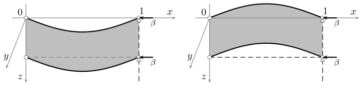
Figure 3. Symmetric in-phase unimodal solutions $(\alpha_{1,1}^{\pm},\alpha_{1,1}^{\pm})$.

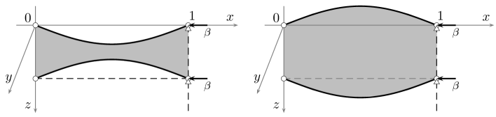
Figure 4. Symmetric out-of-phase unimodal solutions $(\alpha_{1,2}^{\pm},\alpha_{1,2}^{\mp})$.

Figure 5. Nonsymmetric out-of-phase unimodal solutions $(\alpha_{1,3}^{\pm},\alpha_{1,4}^{\mp})$.

Figure 6. Nonsymmetric out-of-phase unimodal solutions $(\alpha_{1,4}^{\pm},\alpha_{1,3}^{\mp})$.

Appendix: Dimensionless Models of Double-Beam Systems

Let us consider a thin and elastic Woinowsky-Krieger beam of natural length $\ell>0$, uniform cross section $\Omega$, and thickness $0<h\ll\ell$. The beam is supposed to be homogeneous, of constant mass density $\rho>0$ per unit volume, and symmetric with respect to the vertical plane ($\xi$-$z$). Hence, we can restrict our attention to its rectangular section lying in the plane $y=0$. Identifying the beam with such a section, we assume that its middle line at rest occupies the interval $[0,\ell]$ of the $\xi$-axis. According to the physical analysis carried out in [8, 13], in the isothermal case the motion equation for the vertical deflection of the midline of the beam

$$U:(\xi,\tau)\in[0,\ell]\times\mathbb{R}^{+}\mapsto\mathbb{R}$$

reads

$$\mathfrak{L}U-\frac{Eh}{2\ell^{2}(1-\nu^{2})}\bigg{(}2D+\int_{0}^{\ell}|\partial_{\xi}U(s)|^{2}\,{\rm d}s\bigg{)}\partial_{\xi\xi}U=\frac{G}{\ell|\Omega|}.$$

Here,

$$\mathfrak{L}=\rho\partial_{\tau\tau}-\frac{\rho h^{2}}{12}\partial_{\tau\tau\xi\xi}+\frac{Eh^{3}}{12\ell(1-\nu^{2})}\,\partial_{\xi\xi\xi\xi}$$

denotes the evolution operator, while

• $|\Omega|>0$ is the area of the cross section,

• $E>0$ is the Young modulus (force per unit area),

• $\nu\in(-1,\frac{1}{2})$ is the Poisson ratio, which is negative for auxetic materials,

• $D\in\mathbb{R}$ is the axial displacement at the right end of the beam,

• $G:[0,\ell]\times\mathbb{R}^{+}\to\mathbb{R}$ is the vertical body force applied on the section $\Omega$.

We point out that the model is obtained by supposing the beam slender (i.e. $h\ll\ell$), and the modulus of the axial displacement $D$ small when compared to the length of the beam (i.e. $|D|\ll\ell$ as well). See also [4, 5, 19] for more details.

Assuming that $G$ is due to the distributed and mutual elastic action exerted between two equal Woinowsky-Krieger beams with vertical deflections $U=U(\xi,\tau)$ and $V=V(\xi,\tau)$, respectively, we let

$$G(\xi,\tau)=-\varkappa\big{[}U(\xi,\tau)-V(\xi,\tau)\big{]},$$

being $\varkappa>0$ the uniform stiffness (force per unit length) of the elastic core. In this situation, the model describing the motion of the resulting elastically-coupled extensible double-beam nonlinear system becomes

$$\begin{cases}\displaystyle\mathfrak{L}U-\frac{Eh}{2\ell^{2}(1-\nu^{2})}\Big{(}2D+\int_{0}^{\ell}|\partial_{\xi}U(s)|^{2}\,{\rm d}s\Big{)}\,\partial_{\xi\xi}U+\frac{\varkappa}{\ell|\Omega|}(U-V)=0,\\ \vskip 3.69885pt\cr\displaystyle\mathfrak{L}V-\frac{Eh}{2\ell^{2}(1-\nu^{2})}\Big{(}2D+\int_{0}^{\ell}|\partial_{\xi}V(s)|^{2}\,{\rm d}s\Big{)}\,\partial_{\xi\xi}V-\frac{\varkappa}{\ell|\Omega|}(U-V)=0.\end{cases}$$

In order to rewrite the system in dimensionless form, we exploit the fact that the two beams have the same structural parameters. In particular, $\ell$ is viewed as the common characteristic length of the beams, while the characteristic time $\tau_{0}$ is obtained by means of the well-known shear wave velocity $c_{0}$ in bulk elasticity, given by

$$c_{0}=\sqrt{\frac{E}{2\rho(1+\nu)}}.$$

Then, the characteristic time $\tau_{0}$ is equal to the ratio $\ell/c_{0}$. Explicitly,

$$\tau_{0}=\sqrt{\frac{2\ell^{2}\rho(1+\nu)}{E}}.$$

Consequently, introducing the dimensionless space and time variables

$$x=\frac{\xi}{\ell}\in[0,1]t=\frac{\tau}{\tau_{0}}\in\mathbb{R}^{+},$$

along with the rescaled unknowns $u,v:[0,1]\times\mathbb{R}^{+}\to\mathbb{R}$ defined as

$$u(x,t)=\frac{U(\ell x,\tau_{0}t)}{\ell}v(x,t)=\frac{V(\ell x,\tau_{0}t)}{\ell},$$

we end up with the dimensionless model

$$\begin{cases}\displaystyle\frac{\ell(1-\nu)}{h}\Big{(}\partial_{tt}-\frac{h^{2}}{12\ell^{2}}\partial_{ttxx}\Big{)}u+\delta\partial_{xxxx}u-\big{(}\chi+\|\partial_{x}u\|^{2}\big{)}\partial_{xx}u+\kappa(u-v)=0,\\ \vskip 4.83694pt\cr\displaystyle\frac{\ell(1-\nu)}{h}\Big{(}\partial_{tt}-\frac{h^{2}}{12\ell^{2}}\partial_{ttxx}\Big{)}v+\delta\partial_{xxxx}v-\big{(}\chi+\|\partial_{x}v\|^{2}\big{)}\partial_{xx}v-\kappa(u-v)=0,\end{cases}$$

where $\|\cdot\|$ denotes the $L^{2}$-norm on the unit interval $[0,1]$, and

$$\delta=\frac{h^{2}}{6\ell^{2}}>0,\qquad\chi=\frac{2D}{\ell}\in\mathbb{R},\qquad\kappa=\frac{2\varkappa\ell^{2}(1-\nu^{2})}{E|\Omega|h}>0.$$

Under reasonably physical assumptions on the stiffness $\varkappa$ of the elastic core, and since $D$ and $h$ are comparable, we may conclude that $|\chi|$ and $\kappa$ share the same order of magnitude $h/\ell$, whereas $\delta$ is much smaller. Accordingly, $|{\chi}/{\delta}|$ and ${\kappa}/{\delta}$ may assume large values, for their order of magnitude is $\ell/h\gg 1$. Hence, all the stationary solutions exhibited in this paper are physically consistent.

References

- [1] I.V. Andrianov, On the theory of berger plates, J. Appl. Math. Mech. 47 (1983), 142–144.
- [2] J.M. Ball, Stability theory for an extensible beam, J. Differential Equations 14 (1973), 399–418.
- [3] I. Bochicchio and E. Vuk, Buckling and longterm dynamics of a nonlinear model for the extensible beam, Math. Comput. Modelling 51 (2010), 833–846.
- [4] P.G. Ciarlet, A justification of the von Krmn equations, Arch. Rational Mech. Anal. 73 (1980), 349–389.
- [5] P.G. Ciarlet and L. Gratie, From the classical to the generalized von Krmn and Marguerre-von Krmn equations, J. Comput. Appl. Math. 190 (2006), 470–486.
- [6] A. Ciekot and S. Kukla, Frequency analysis of a double-nanobeam-system, J. Appl. Math. Comput. Mech. 13 (2014), 23–31.
- [7] M. Coti Zelati, Global and exponential attractors for the singularly perturbed extensible beam, Discrete Contin. Dyn. Syst. 25 (2009), 1041–1060.
- [8] M. Coti Zelati, C. Giorgi and V. Pata, Steady states of the hinged extensible beam with external load, Math. Models Methods Appl. Sci. 20 (2010), 43–58.
- [9] J.M. Davies, Lightweight sandwich construction, Wiley-Blackwell, Oxford, 2001.
- [10] R.W. Dickey, Free vibrations and dynamic buckling of the extensible beam, J. Math. Anal. Appl. 29 (1970), 443–454.
- [11] R.W. Dickey, Dynamic stability of equilibrium states of the extensible beam, Proc. Amer. Math. Soc. 41 (1973), 94–102.
- [12] A. Eden and A.J. Milani, Exponential attractors for extensible beam equations, Nonlinearity 6 (1993), 457–479.
- [13] C. Giorgi and M.G. Naso, Modeling and steady state analysis of the extensible thermoelastic beam, Math. Comp. Modelling 53 (2011), 896–908.
- [14] C. Giorgi, V. Pata and E. Vuk, On the extensible viscoelastic beam, Nonlinearity 21 (2008), 713–733.
- [15] P. Holmes and J. Marsden, A partial differential equation with infinitely many periodic orbits: chaotic oscillations of a forced beam, Arch. Rational Mech. Anal. 76 (1981), 135–165.
- [16] N. Kamiya, Governing equations for large deflections of sandwich plates, AIAA Journal 14 (1976), 250–253.
- [17] S.G. Kelly and S. Srinivas, Free vibrations of elastically connected stretched beams, J. Sound Vibration 326 (2009), 883–893.
- [18] W. Lacarbonara, Nonlinear structural mechanics. Theory, dynamical phenomena and modeling, Springer, New York, 2013.
- [19] J.E. Lagnese and J.L. Lions, Modelling analysis and control of thin plates, Masson, Paris, 1988.
- [20] P.J. McKenna, Oscillations in suspension bridges, vertical and torsional, Discrete Contin. Dyn. Syst. Ser. S 7 (2014), 785–791.
- [21] T. Murmu and S. Adhikari, Axial instability of a double-nanobeam-systems, Phys. Lett. A 375 (2011), 601–608.
- [22] Z. Oniszczuk, Forced transverse vibrations of an elastically connected complex simply supported double-beam system, J. Sound Vibration 264 (2003), 273–286.
- [23] F.J. Plantema, Sandwich construction: the bending and buckling of sandwich beams, plates, and shells, John Wiley and Sons, New York, 1966.
- [24] E.L. Reiss and B.J. Matkowsky, Nonlinear dynamic buckling of a compressed elastic column, Quart. Appl. Math. 29 (1971), 245–260.
- [25] R. Taylor and A. Wiles, Ring-theoretic properties of certain Hecke algebras, Ann. of Math. 141 (1995), 553–572.
- [26] H.V. Vu, A.M. Ordez and B.K. Karnopp, Vibration of a double-beam system, J. Sound Vibration 229 (2000), 807–822.
- [27] D.H. Wang and G.F. Wang, Surface effects on the vibration and buckling of double-nanobeam-systems, Journal of Nanomaterials vol. 2011 (2011), Article ID 518706, 7 pages.
- [28] A. Wiles, Modular elliptic curves and Fermat’s last theorem, Ann. of Math. 141 (1995), 443–551.
- [29] S. Woinowsky-Krieger, The effect of an axial force on the vibration of hinged bars, J. Appl. Mech. 17 (1950), 35–36.
- [30] D. Zenkert, An introduction to sandwich construction, EMAS Publications, West Midlands, United Kingdom, 1995.
- [31] Y.Q. Zhang, Y. Lu and G.W. Ma, Effect of compressive axial load on forced transverse vibrations of a double-beam system, Int. J. Mech. Sci. 50 (2008), 299–305.
- [32] Y.Q. Zhang, Y. Lu, S.L. Wang and X. Liu, Vibration and buckling of a double-beam system under compressive axial loading, J. Sound Vibration 318 (2008), 341–352.