Comparison principle for stochastic heat equation on $\mathbb{R}^{d}$

Abstract

We establish the strong comparison principle and strict positivity of solutions to the following nonlinear stochastic heat equation on $\mathbb{R}^{d}$

$$\left(\frac{\partial}{\partial t}-\frac{1}{2}\Delta\right)u(t,x)=\rho(u(t,x))\>\dot{M}(t,x),$$

for measure-valued initial data, where $\dot{M}$ is a spatially homogeneous Gaussian noise that is white in time and $\rho$ is Lipschitz continuous. These results are obtained under the condition that $\int_{\mathbb{R}^{d}}(1+|\xi|^{2})^{\alpha-1}\hat{f}(\text{d}\xi)<\infty$ for some $\alpha\in(0,1]$, where $\hat{f}$ is the spectral measure of the noise. The weak comparison principle and nonnegativity of solutions to the same equation are obtained under Dalang’s condition, i.e., $\alpha=0$. As some intermediate results, we obtain handy upper bounds for $L^{p}(\Omega)$-moments of $u(t,x)$ for all $p\geq 2$, and also prove that $u$ is a.s. Hölder continuous with order $\alpha-\epsilon$ in space and $\alpha/2-\epsilon$ in time for any small $\epsilon>0$.

Keywords. Stochastic heat equation; parabolic Anderson model; space-time Hölder regularity; spatially homogeneous noise; comparison principle; measure-valued initial data.

AMS 2010 subject classification. Primary 60H15; Secondary 35R60, 60G60.

1 Introduction

In this paper, we study the sample-path comparison principle, or simply comparison principle of the solutions to the following stochastic heat equation (SHE) with rough initial conditions,

$$\begin{cases}\displaystyle\left(\frac{\partial}{\partial t}-\frac{1}{2}\Delta\right)u(t,x)=\rho(u(t,x))\>\dot{M}(t,x),&x\in\mathbb{R}^{d},\;t>0,\\ \displaystyle\quad u(0,\cdot)=\mu(\cdot).\end{cases}$$ (1.1)

In this equation, $\rho$ is assumed to be a globally Lipschitz continuous function. The linear case, i.e., $\rho(u)=\lambda u$, is called the parabolic Anderson model (PAM) [3]. The noise $\dot{M}$ is a Gaussian noise that is white in time and homogeneously colored in space. Informally,

$$\mathbb{E}\left[\dot{M}(t,x)\dot{M}(s,y)\right]=\delta_{0}(t-s)f(x-y)$$

where $\delta_{0}$ is the Dirac delta measure with unit mass at zero and $f$ is a “correlation function” i.e., a nonnegative and nonnegative definite function that is not identically zero. The Fourier transform of $f$ is denoted by $\hat{f}$

$$\hat{f}(\xi)=\mathcal{F}f(\xi)=\int_{\mathbb{R}^{d}}\exp\left(-i\>\xi\cdot x\right)f(x)\mathrm{d}x.$$

In general, $\hat{f}$ is again a nonnegative and nonnegative definite measure, which is usually called the spectral measure. The precise meaning of the “rough initial conditions/data” are specified as follows. We first note that by the Jordan decomposition, any signed Borel measure $\mu$ can be decomposed as $\mu=\mu_{+}-\mu_{-}$ where $\mu_{\pm}$ are two non-negative Borel measures with disjoint support. Denote $|\mu|:=\mu_{+}+\mu_{-}$. The rough initial data refers to any signed Borel measure $\mu$ such that

$$\int_{\mathbb{R}^{d}}e^{-a|x|^{2}}|\mu|(\mathrm{d}x)<+\infty\;,\quad\text{for all $a>0$}\;,$$ (1.2)

where $|x|=\sqrt{x_{1}^{2}+\dots+x_{d}^{2}}$ denotes the Euclidean norm. It is easy to see that condition (1.2) is equivalent to the condition that the solution to the homogeneous equation – $J_{0}(t,x)$ defined in (1.6) below – exists for all $t>0$ and $x\in\mathbb{R}^{d}$.

The comparison principle refers to the property that if two initial conditions are comparable, then the corresponding solutions to the stochastic partial differential equations are also comparable. For any Borel measure $\mu$ on $\mathbb{R}^{d}$, “$\mu\geq 0$” has its obvious meaning that $\mu$ is a nonnegative measure and “$\mu>0$” refers to the fact that $\mu\geq 0$ and $\mu$ is nonvanishing, i.e., $\mu\neq 0$. Let $u_{1}$ and $u_{2}$ be two solutions starting from two measures $\mu_{1}$ and $\mu_{2}$, respectively. We say that (1.1) satisfies the weak comparison principle if $u_{1}(t,x)\leq u_{2}(t,x)$ a.s. for all $t>0$ and $x\in\mathbb{R}^{d}$ whenever $\mu_{1}\leq\mu_{2}$. Similarly, we say that (1.1) satisfies the strong comparison principle if $u_{1}(t,x)<u_{2}(t,x)$ for all $t>0$ and $x\in\mathbb{R}^{d}$ a.s. whenever $\mu_{1}<\mu_{2}$. Note that when $\rho(u)=\lambda u$, it is relatively easier to establish the weak comparison principle since the solution can be approximated by its regularized version, which admits a Feynman-Kac formula; see [16, 17, 18].

Most strong comparison principles are obtained through Mueller’s original work [19], where he proved the case when $d=1$, $\dot{M}$ is the space-time white noise, $\rho(u)=|u|^{\gamma}$ (for all $\gamma\leq 1$), and the initial data is a bounded function. In [22], Shiga studied the same equation as that in [19] except that $\rho$ is assumed to be Lipschitz and there can be a drift term. By using concentration of measure arguments for discrete directed polymers in Gaussian environments, Flores established in [13] the strict positivity of solution to 1-d PAM with Dirac delta initial data. Following arguments by Mueller and Shiga, Chen and Kim extended these results in [8] to allow both fractional Laplace operators and rough initial data. Recently, by using paracontrolled distributions, Gubinelli and Perkowski gave an intrinsic proof of the strict positivity; see [15]. Their proof does not depend on the details of noise, though they require the initial data to be a function that is strict positive anywhere.

When $d\geq 2$, in order to study a random field solution, the noise has to have some color in space. Equation (1.1) has been much studied since the introduction by Dawson and Salehi [12] as a model for the growth of a population in a random environment. In [10, 11], it is shown that if the initial condition is a bounded function, and under some integrability condition on $\hat{f}$, now called Dalang’s condition, i.e.,

$$\Upsilon(\beta):=(2\pi)^{-d}\int_{\mathbb{R}^{d}}\frac{\hat{f}(\mathrm{d}\xi)}{\beta+|\xi|^{2}}<+\infty\quad\text{for some and hence for all $\beta>0$,}$$ (1.3)

there is a unique random field solution to equation (1.1). This equation has been extensively studied; see, e.g., [6, 14, 16, 18]. Recently, Chen and Kim showed that Dalang’s condition (1.3) also guarantees an $L^{2}(\Omega)$-continuous random field solution starting from rough initial conditions; see [7]. To the best of our knowledge, comparison principle in this setting is much less known, though people believe that it is true. In [23], Tessitore and Zabczyk proved the strict positivity for the case when $\hat{f}$ belongs to $L^{p}(\mathbb{R}^{d})$ for some $p\in[1,d/(d-2))$. Clearly, this condition excludes the important Riesz kernel case, i.e., $f(x)=|x|^{-\beta}$ with $\beta\in(0,2\wedge d)$. Indeed, we will show that under Dalang’s condition (1.3), if $\rho(0)=0$, then the solution $u(t,x)$ starting from any nonnegative rough initial data is a.s. nonnegative for any $t>0$ and $x\in\mathbb{R}^{d}$. Moreover, if the nonnegative rough initial data is nonvanishing and $f$ satisfies

$$\int_{\mathbb{R}^{d}}\frac{\hat{f}(\mathrm{d}\xi)}{\left(1+|\xi|^{2}\right)^{1-\alpha}}<\infty,\quad\text{for some $\alpha\in(0,1]$,}$$ (1.4)

then we are able to establish the strict positivity of $u(t,x)$ through the following small-ball probability estimate:

$$\mathbb{P}\left(u(t,x)<\epsilon\right)\leq A\exp\left(-A|\log\epsilon|^{\alpha}\left(\log|\log\epsilon|\right)^{1+\alpha}\right)\,.$$

Similar small-ball probabilities in various settings can be found in [8, 9, 13, 20]. These nonnegativity statements can be translated into comparison statements by considering $v=u_{1}-u_{2}$.

Condition (1.4) is natural since in a recent paper [6], it is shown that Dalang’s condition (1.3) alone cannot guarantee the existence of a continuous version of the solution. There might be solutions that behave so badly that they may hit zero. Whether this phenomenon does happen is still not clear to us and it is left for future exploration. For the moment, we are content with this slightly strong condition (1.4). Indeed, if the initial condition is a bounded function, Sanz-Solé and Sarrà [21] showed that condition (1.4) guarantees that the solution is a.s. Hölder continuous with order $\alpha-\epsilon$ in space and $\alpha/2-\epsilon$ in time for any small $\epsilon>0$. In this paper, we have extended this result for rough initial conditions. The space-time white noise case is proved in [5].

In all these studies, the moment bounds/formulas play an important role. The upper bounds for the second moments under Dalang’s condition (1.3) for rough initial conditions is obtained in [7]. In this paper, we extend this bound to obtain similar upper bounds for all $p$-th moments, $p\geq 2$. Using these moments upper bounds, we establish the (weak) comparison principle, whose property is assumed in [7] in order to obtain some nontrivial lower bounds for the second moments. Note when $\rho(u)=\lambda u$, the $p$-th moment admits a Feynman-Kac representation, which has been exploited to study the intermittency phenomenon in [16, 17, 18].

1.1 Main results

The solution to (1.1) is understood as the mild form

$$u(t,x) =J_{0}(t,x)+\int_{0}^{t}\int_{\mathbb{R}^{d}}G(t-s,x-y)\rho(u(s,y))M(\mathrm{d}s,\mathrm{d}y),$$ (1.5)

where $J_{0}(t,x)$ is the solution to the homogeneous equation

$$J_{0}(t,x):=\left(\mu*G(t,\cdot)\right)(x)=\int_{\mathbb{R}^{d}}G(t,x-y)\mu(\mathrm{d}y)$$ (1.6)

and

$$G(t,x)=\left(2\pi t\right)^{-d/2}\exp\left(-\frac{|x|^{2}}{2t}\right).$$ (1.7)

We will prove seven theorems listed as follows:

Theorem 1.1 (Weak comparison principle).

Assume that $f$ satisfies Dalang’s condition (1.3). Let $u_{1}(t,x)$ and $u_{2}(t,x)$ be two solutions to (1.1) with the initial measures $\mu_{1}$ and $\mu_{2}$ that satisfy (1.2), respectively. If $\mu_{1}\leq\mu_{2}$, then

$$\mathbb{P}\left(u_{1}(t,x)\leq u_{2}(t,x)\right)=1\,,\quad\text{for all}\ t\geq 0\ \text{and}\ x\in\mathbb{R}^{d}\,.$$ (1.8)

Moreover, if the paths of $u_{1}(t,x)$ and $u_{2}(t,x)$ are a.s. continuous, then

$$\mathbb{P}\left(u_{1}(t,x)\leq u_{2}(t,x)\ \text{for all}\ t\geq 0\ \text{and}\ x\in\mathbb{R}^{d}\right)=1\,.$$ (1.9)

If $\rho(0)=0$, then $u\equiv 0$ is the unique solution to (1.1) starting from $\mu=0$. Hence, we have the following corollary:

Corollary 1.2 (Nonnegativity).

Assume that $f$ satisfies Dalang’s condition (1.3) and $\rho(0)=0$. Let $u$ be the solution to (1.1) with the initial measure $\mu$ that satisfies (1.2). If $\mu\geq 0$, then

$$\mathbb{P}\left(u(t,x)\geq 0\right)=1\,,\quad\text{for all}\ t\geq 0\ \text{and}\ x\in\mathbb{R}^{d}\,.$$ (1.10)

Moreover, if the path of $u(t,x)$ are a.s. continuous, then

$$\mathbb{P}\left(u(t,x)\geq 0\ \text{for all}\ t\geq 0\ \text{and}\ x\in\mathbb{R}^{d}\right)=1\,.$$ (1.11)

Theorem 1.3 (Strong comparison principle).

Assume that $f$ satisfies (1.4) for some $\alpha\in(0,1]$. Let $u_{1}(t,x)$ and $u_{2}(t,x)$ be two solutions to (1.1) with the initial data $\mu_{1}$ and $\mu_{2}$, respectively. Then the fact that $\mu_{1}<\mu_{2}$ implies

$$\mathbb{P}\left(u_{1}(t,x)<u_{2}(t,x)\ \text{for all}\ t>0\ \text{and}\ x\in\mathbb{R}^{d}\>\right)=1.$$ (1.12)

Theorem 1.4 (Strict positivity).

Assume that $f$ satisfies (1.4) for some $\alpha\in(0,1]$ and $\rho(0)=0$. Let $u$ be the solution to (1.1) with initial measure $\mu>0$ that satisfies (1.2). Then for any compact set $K\subset\mathbb{R}_{+}^{*}\times\mathbb{R}^{d}$, there exists a finite constant $A>0$ which only depends on $K$ such that for all $\epsilon>0$ small enough,

$$\mathbb{P}\left(\inf_{(t,x)\in K}u(t,x)<\epsilon\right)\leq A\exp\left(-A|\log\epsilon|^{\alpha}\left(\log|\log\epsilon|\right)^{1+\alpha}\right)\,.$$ (1.13)

In order to establish the above results, we need to prove the following four theorems, which are of interest by themselves. The first result is a general moment bound. This provides us with a very handy tool in studying various properties of the solution to (1.1). This result extends the previous work [7] from the two-point correlation function to higher moments. Let $\operatorname{Lip}_{\rho}>0$ be the Lipschitz constant for $\rho$. See Section 3 for the proof.

Theorem 1.5 (Moment bounds).

Under Dalang’s condition (1.3), if the initial data $\mu$ is a signed measure that satisfies (1.2), then the solution $u$ to (1.1) for any given $t>0$ and $x\in\mathbb{R}^{d}$ is in $L^{p}(\Omega)$, $p\geq 2$, and

$$\left|\left|u(t,x)\right|\right|_{p}\leq\sqrt{2}\left[\operatorname{\overline{\varsigma}}+\sqrt{2}\left(|\mu|*G(t,\cdot)\right)(x)\right]H\left(t;\gamma_{p}\right)^{1/2},$$ (1.14)

where $\operatorname{\overline{\varsigma}}=|\rho(0)|/\operatorname{Lip}_{\rho}$ and $\gamma_{p}=32p\operatorname{Lip}_{\rho}^{2}$ and $H(t;\gamma_{p})$ is defined in (2.5) below. Moreover, if for some $\alpha\in(0,1]$ condition (1.4) is satisfied, then when $p\geq 2$ is large enough, there exists some constant $C>0$ such that

$$\left|\left|u(t,x)\right|\right|_{p}\leq C\Big{[}\>\operatorname{\overline{\varsigma}}+\left(|\mu|*G(t,\cdot)\right)(x)\Big{]}\exp\left(Cp^{1/\alpha}t\right)\,.$$ (1.15)

The second result is about the sample-path regularity under condition (1.4) for rough initial conditions. This result is used to obtain a large deviation estimates in proving the strong comparison principle. See Section 4 for its proof.

Theorem 1.6 (Hölder regularity).

Suppose that $\mu$ is any measure that satisfies (1.2) and $f$ satisfies (1.4) for some $\alpha\in(0,1]$. Then the solution to (1.1) starting from $\mu$ is a.s. $\beta_{1}$-Hölder continuous in time and $\beta_{2}$-Hölder continuous in space on $(0,\infty)\times\mathbb{R}^{d}$ with

$$\beta_{1}\in\left(0,\alpha/2\right)\quad\text{and}\quad\beta_{2}\in\left(0,\alpha\right).$$

The third theorem consists of two approximation results, which are used to establish the weak comparison principle. The first one says that we can approximate a solution starting from a rough initial data by solutions starting from smooth and bounded initial conditions. This result allows us to pass from the weak comparison principle for $L^{\infty}(\mathbb{R}^{d})$-valued initial data to that for rough initial data. In the second approximation, we mollify the noise and establish an uniform $L^{2}(\Omega)$-limit. See Section 5 for the proof.

Theorem 1.7 (Two approximations).

Assume that $f$ satisfies Dalang’s condition (1.3).

(1) Suppose that the initial measure $\mu$ satisfies (1.2). If $u(t,x)$ and $u_{\epsilon}(t,x)$ be the solutions to (1.1) starting from $\mu$ and $((\mu\>\psi_{\epsilon})*G(\epsilon,\cdot))(x)$, respectively, where

$$\psi_{\epsilon}(x)={{\rm 1\mkern-1.5mu}\!{\rm I}}_{\{|x|\leq 1/\epsilon\}}+\left(1+1/\epsilon-|x|\right){{\rm 1\mkern-1.5mu}\!{\rm I}}_{\{1/\epsilon<|x|\leq 1+1/\epsilon\}},$$ (1.16)

then

$$\lim_{\epsilon\rightarrow 0_{+}}\left|\left|u(t,x)-u_{\epsilon}(t,x)\right|\right|_{2}=0,\quad\text{for all $t>0$ and $x\in\mathbb{R}^{d}$.}$$

(2) Let $\phi$ be any continuous, nonnegative and nonnegative definite function on $\mathbb{R}^{d}$ with compact support such that $\int_{\mathbb{R}^{d}}\phi(x)\mathrm{d}x=1$. Let $u$ be the solution to (1.1) starting from a bounded initial data, i.e., $\mu(\mathrm{d}x)=g(x)\mathrm{d}x$ with $g\in L^{\infty}(\mathbb{R}^{d})$. If $u^{\epsilon}$ is the solution to the following mollified equation

$$\frac{\partial}{\partial t}u_{\epsilon}(t,x)=\frac{1}{2}\Delta u_{\epsilon}(t,x)+\rho(u_{\epsilon}(t,x))\dot{M}^{\epsilon}(t,x)\,,$$ (1.17)

with the same initial condition $u^{\epsilon}(0,\cdot)=\mu$ as $u$, where

$$M^{\epsilon}(\mathrm{d}s,\mathrm{d}x)=\int_{\mathbb{R}^{d}}\phi_{\epsilon}(x-y)M(\mathrm{d}s,\mathrm{d}y)\mathrm{d}x\,,$$ (1.18)

and $\phi_{\epsilon}(x)=\epsilon^{-d}\phi(x/\epsilon)$, then

$$\lim_{\epsilon\rightarrow 0_{+}}\sup_{x\in\mathbb{R}^{d}}\left|\left|u(t,x)-u_{\epsilon}(t,x)\right|\right|_{2}=0,\quad\text{for all $t>0$.}$$ (1.19)

Remark 1.8.

One can always find one example of such function $\phi$ in part (2) of Theorem 1.7, e.g., $\phi(x)=\prod_{i=1}^{d}\left(1-|x_{i}|\right){{\rm 1\mkern-1.5mu}\!{\rm I}}_{\{|x_{i}|\leq 1\}}$ whose Fourier transform is nonnegative: $\hat{\phi}(\xi)=2^{d}\prod_{j=1}^{d}\xi_{j}^{-2}(1-\cos(\xi_{j}))\geq 0$.

The last result shows that the solution $u(t,x)$ to (1.1) converges to its initial data $\mu$ weakly as $t\rightarrow 0$. This result is used to establish the strong comparison principle for measure-valued initial data given that for function-valued initial data. See Section 6 for the proof. Let $C_{c}(\mathbb{R}^{d})$ be the set of continuous functions with compact support.

Theorem 1.9.

Under Dalang’s condition (1.3), if $u(t,x)$ be the solution to (1.1) starting from a Borel measure $\mu$ that satisfies (1.2), then

$$\lim_{t\rightarrow 0}\int_{\mathbb{R}^{d}}u(t,x)\phi(x)\mathrm{d}x=\int_{\mathbb{R}^{d}}\phi(x)\mu(\mathrm{d}x)\qquad\text{in $L^{2}(\Omega)$ for all $\phi\in C_{c}(\mathbb{R}^{d})$,}$$ (1.20)

where the probability space is introduced in Section 2.

This paper is organized as follows: After some preliminaries in Section 2, we first prove the moment bounds, Theorem 1.5, in Section 3. Using these moment bounds, we proceed to establish the Hölder regularity, Theorem 1.6, in Section 4. Then in Section 5 we prove Theorem 1.7 for the two approximations. The weak limit as $t$ goes to zero, i.e., Theorem 1.9, is proved in Section 6. With these preparation, we prove the weak comparison principle, Theorem 1.1, in Section 7. Finally, in Section 8 we prove both the strong comparison principle (Theorem 1.3) and the strict positivity (Theorem 1.4). Some technical lemmas are given in Appendix. Throughout this paper, $C$ will denote a generic constant which may vary at each occurrence.

2 Some preliminaries

2.1 Definition and existence of a solution

Recall that a spatially homogeneous Gaussian noise that is white in time is an $L^{2}(\Omega)$-valued mean zero Gaussian process on a complete probability space $\left(\Omega,\mathcal{F},\mathbb{P}\right)$

$$\left\{F(\psi):\>\psi\in C_{c}^{\infty}\left([0,\infty)\times\mathbb{R}^{d}\right)\>\right\},$$

such that

$$\mathbb{E}\left[F(\psi)F(\phi)\right]=\int_{0}^{\infty}\mathrm{d}s\iint_{\mathbb{R}^{2d}}\psi(s,x)\phi(s,y)f(x-y)\mathrm{d}x\mathrm{d}y.$$

Let $\mathcal{B}_{b}(\mathbb{R}^{d})$ be the collection of Borel measurable sets with finite Lebesgue measure. As in Dalang-Walsh theory [10, 24], one can extend $F$ to a $\sigma$-finite $L^{2}(\Omega)$-valued martingale measure $B\mapsto F(B)$ defined for $B\in\mathcal{B}_{b}(\mathbb{R}_{+}\times\mathbb{R}^{d})$. Then define

$$M_{t}(B):=F\left([0,t]\times B\right),\quad B\in\mathcal{B}_{b}(\mathbb{R}^{d}).$$

Let $(\mathcal{F}_{t},t\geq 0)$ be the natural filtration generated by $M_{\cdot}(\cdot)$ and augmented by all $\mathbb{P}$-null sets $\mathcal{N}$ in $\mathcal{F}$, i.e.,

$$\mathcal{F}_{t}:=\sigma\left(M_{s}(A):\>0\leq s\leq t,A\in\mathcal{B}_{b}\left(\mathbb{R}^{d}\right)\right)\vee\mathcal{N},\quad t\geq 0,$$

Then for any adapted, jointly measurable (with respect to $\mathcal{B}\left((0,\infty)\times\mathbb{R}^{d}\right)\times\mathcal{F}$) random field $\{X(t,x):t>0,x\in\mathbb{R}^{d}\}$ such that

$$\int_{0}^{\infty}\mathrm{d}s\iint_{\mathbb{R}^{2d}}\mathrm{d}x\mathrm{d}y\>\left|\left|X(s,y)X(s,x)\right|\right|_{\frac{p}{2}}f(x-y)<\infty,$$

the stochastic integral

$$\int_{0}^{\infty}\int_{\mathbb{R}^{d}}X(s,y)M(\mathrm{d}s,\mathrm{d}y)$$

is well-defined in the sense of Dalang-Walsh. Here we only require the joint-measurability instead of predictability; see Proposition 2.2 in [7] for this case or Proposition 3.1 in [4] for the space-time white noise case. Throughout this paper, $\left|\left|\cdot\right|\right|_{p}$ denotes the $L^{p}(\Omega)$-norm.

We formally write the SPDE (1.1) in the integral form

$$u(t,x)=J_{0}(t,x)+I(t,x)$$ (2.1)

where

$$I(t,x):=\iint_{[0,t]\times\mathbb{R}^{d}}G(t-s,x-y)\rho(u(s,y))M(\mathrm{d}s,\mathrm{d}y).$$

The above stochastic integral is understood in the sense of Walsh [10, 24].

Definition 2.1.

A process $u=\left(u(t,x),\>(t,x)\in(0,\infty)\times\mathbb{R}^{d}\right)$ is called a random field solution to (1.1) if

1. $u$ is adapted, i.e., for all $(t,x)\in(0,\infty)\times\mathbb{R}^{d}$, $u(t,x)$ is $\mathcal{F}_{t}$-measurable;

2. $u$ is jointly measurable with respect to $\mathcal{B}\left((0,\infty)\times\mathbb{R}^{d}\right)\times\mathcal{F}$;

3. $\left|\left|I(t,x)\right|\right|_{2}<+\infty$ for all $(t,x)\in(0,\infty)\times\mathbb{R}^{d}$;

4. $I$ is $L^{2}(\Omega)$-continuous, i.e., the function $(t,x)\mapsto I(t,x)$ mapping $(0,\infty)\times\mathbb{R}^{d}$ into $L^{2}(\Omega)$ is continuous;

5. $u$ satisfies (2.1) a.s., for all $(t,x)\in(0,\infty)\times\mathbb{R}^{d}$.

Theorem 2.2 (Theorem 2.4 in [7]).

If the initial data $\mu$ satisfies (1.2), then under Dalang’s condition (1.3), SPDE (1.1) has a unique (in the sense of versions) random field solution $\left\{u(t,x):t>0,x\in\mathbb{R}^{d}\right\}$ starting from $\mu$. This solution is $L^{2}(\Omega)$-continuous.

2.2 Some special functions

We first introduce some notation following [7]. Denote

$$k(t):=\int_{\mathbb{R}^{d}}f(z)G(t,z)\mathrm{d}z.$$ (2.2)

By Fourier transform, this function can be written in the following form

$$k(t):=(2\pi)^{-d}\int_{\mathbb{R}^{d}}\hat{f}(\mathrm{d}\xi)\exp\left(-\frac{t|\xi|^{2}}{2}\right).$$ (2.3)

Define $h_{0}(t):=1$ and for $n\geq 1$,

$$h_{n}(t)=\int_{0}^{t}\mathrm{d}s\>h_{n-1}(s)k(t-s).$$ (2.4)

Let

$$H(t;\gamma):=\sum_{n=0}^{\infty}\gamma^{n}h_{n}(t).$$ (2.5)

This function is defined through the correlation function $f$. The following lemma tells us that this function has an exponential bound.

Lemma 2.3 (Lemma 2.5 in [7] or Lemma 3.8 in [2]).

For all $t\geq 0$ and $\gamma\geq 0$,

$$\limsup_{t\rightarrow\infty}\frac{1}{t}\log H(t;\gamma)\leq\inf\left\{\beta>0:\>\Upsilon\left(\beta\right)<\frac{1}{\gamma}\right\}.$$ (2.6)

2.3 A remark on two recursions

The purpose of this part is to compare the two recursions (3.1) and (2.10) below. While Lemma 3.1 gives an easy to use upper bound, Lemma 2.4 is sharper and used in [7] to obtain lower bounds for the second moment. Recursion (2.10) and its conclusion (2.12) will play a crucial role in the proof of part (1) of Theorem 1.7.

In order to make this statement clear, we need to introduce some notation. For $h,w:\mathbb{R}_{+}\times\mathbb{R}^{3d}\mapsto\mathbb{R}$, define the (asymmetric convolution) operation “$\rhd$”, which depends on $f$, as follows

$$\left(h\rhd w\right)(t,x,x^{\prime};y):=\int_{0}^{t}\mathrm{d}s\iint_{\mathbb{R}^{2d}}\mathrm{d}z\mathrm{d}z^{\prime}\;h(t-s,x-z,x^{\prime}-z^{\prime};y-(z-z^{\prime}))$$ (2.7)

$$\qquad\times w(s,z,z^{\prime};y)\>f(y-(z-z^{\prime}))$$ .

By change of variables,

$$\left(h\rhd w\right)(t,x,x^{\prime};y):=\int_{0}^{t}\mathrm{d}s\iint_{\mathbb{R}^{2d}}\mathrm{d}z\mathrm{d}z^{\prime}\>h(s,z,z^{\prime};y-[(x-z)-(x^{\prime}-z^{\prime})])$$ (2.8)

$$\times w(t-s,x-z,x^{\prime}-z^{\prime};y)\>f(y-[(x-z)-(x^{\prime}-z^{\prime})])$$ .

This operation is associative (see Lemma B.1 in [7])

$$\left(\left(h\rhd w\right)\rhd v\right)(t,x,x^{\prime};y)=\left(h\rhd\left(w\rhd v\right)\right)(t,x,x^{\prime};y).$$

We use the convention that if a function $h$ is defined on $\mathbb{R}_{+}\times\mathbb{R}^{2d}$ instead of $\mathbb{R}_{+}\times\mathbb{R}^{3d}$, when applying the operation $\rhd$ to $h$, it is meant for $h^{\prime}(t,x,x^{\prime};y):=h(t,x,x^{\prime})$.

For $t>0$ and $x,x^{\prime},y\in\mathbb{R}^{d}$, define recursively:

$$\mathcal{L}_{0}(t,x,x^{\prime};y):=G(t,x)G(t,x^{\prime})$$

and for $n\geq 1$,

$$\mathcal{L}_{n}(t,x,x^{\prime};y):=\left(\mathcal{L}_{0}\rhd\mathcal{L}_{n-1}\right)(t,x,x^{\prime};y).$$

For $\lambda\in\mathbb{R}$, Lemma 2.7 of [7] ensures that the following series is well defined

$$\mathcal{K}_{\lambda}(t,x,x^{\prime};y):=\sum_{n=0}^{\infty}\lambda^{2(n+1)}\mathcal{L}_{n}(t,x,x^{\prime};y)\leq\mathcal{L}_{0}(t,x,x^{\prime})H(t;2\lambda^{2}).$$ (2.9)

Then the upper bounds for the two-point correlation function in Theorem 2.4 of [7] can be summarized as the following lemma.

Lemma 2.4.

If for some nonnegative function $J_{*}:\mathbb{R}_{+}\times\mathbb{R}^{2d}\mapsto\mathbb{R}_{+}$ and $\lambda\geq 0$, a function $g:\mathbb{R}_{+}\times\mathbb{R}^{2d}\mapsto\mathbb{R}$ satisfies the following integral inequality

$$\begin{aligned} g(t,x,x^{\prime})\leq J_{*}(t,x,x^{\prime})+\lambda^{2}\int_{0}^{t}\mathrm{d}s\iint_{\mathbb{R}^{2d}}&G(t-s,x-y_{1})G(t-s,x^{\prime}-y_{2})\\ &\times f(y_{1}-y_{2})g(s,y_{1},y_{2})\mathrm{d}y_{1}\mathrm{d}y_{2},\end{aligned}$$ (2.10)

then

$$g(t,x,x^{\prime})\leq J_{*}(t,x,x^{\prime})+\left(\mathcal{K}_{\lambda}\rhd J_{*}\right)(t,x,x^{\prime};0).$$ (2.11)

In particular,

$$\begin{aligned} g(t,x,x^{\prime})\leq J_{*}(t,x,x^{\prime})+H(t;2\lambda^{2})\int_{0}^{t}\mathrm{d}s\iint_{\mathbb{R}^{2d}}&G(t-s,x-y_{1})G(t-s,x^{\prime}-y_{2})\\ &\times f(y_{1}-y_{2})J_{*}(s,y_{1},y_{2})\mathrm{d}y_{1}\mathrm{d}y_{2}.\end{aligned}$$ (2.12)

When the inequality in (2.10) is equality, the conclusion in (2.11) is also an equality.

Proof.

This lemma is proved using the Picard iteration. We need only to prove the case when both inequalities in (2.10) and (2.12) are equalities. Notice that (2.10) (with inequality replaced by equality) can be written as

$$g(t,x,x^{\prime})=J_{*}(t,x,x^{\prime})+\lambda^{2}(\mathcal{L}_{0}\rhd g)(t,x,x^{\prime};0).$$

Let

$$g_{0}(t,x,x^{\prime}):=J_{*}(t,x,x^{\prime}),$$

and for $n\geq 1$,

$$g_{n}(t,x,x^{\prime})=J_{*}(t,x,x^{\prime})+\lambda^{2}\left(\mathcal{L}_{0}\rhd g_{n-1}\right)(t,x,x^{\prime};0).$$ (2.13)

Then by the associativity of the operator $\rhd$, we see that

$$g_{n}(t,x,x^{\prime})=J_{*}(t,x,x^{\prime})+\sum_{k=0}^{n}\lambda^{2(k+1)}\left(\mathcal{L}_{k}\rhd J_{*}\right)(t,x,x^{\prime};0).$$

Therefore,

$$g(t,x,x^{\prime})=\lim_{n\rightarrow\infty}g_{n}(t,x,x^{\prime}) =J_{*}(t,x,x^{\prime})+\sum_{k=0}^{\infty}\lambda^{2(k+1)}\left(\mathcal{L}_{k}\rhd J_{*}\right)(t,x,x^{\prime};0)$$

$$=J_{*}(t,x,x^{\prime})+\left(\mathcal{K}_{\lambda}\rhd J_{*}\right)(t,x,x^{\prime};0)$$

$$\leq J_{*}(t,x,x^{\prime})+H(t;2\lambda^{2})\left(\mathcal{L}_{0}\rhd J_{*}\right)(t,x,x^{\prime};0),$$

where in the last step we have applied the bound for $\mathcal{K}$ in (2.9). This proves Lemma 2.4. ∎

3 Moment bounds (Proof of Theorem 1.5)

While Lemma 2.4 is appropriate for dealing with the two-point correlation function, the corresponding recursion for the $p$-point $(p>2)$ correlation function will be much more complicated. We will instead consider the bounds for the $p$-th moment. The following lemma will play the same role to the $p$-th moment as Lemma 2.4 to the two-point correlation function.

Lemma 3.1.

Suppose that $\mu$ is a signed measure that satisfies (1.2) and let $J_{0}(t,x)$ be the solution to the homogeneous equation (see (1.6)). If a nonnegative function $g:\mathbb{R}_{+}\times\mathbb{R}^{d}\mapsto\mathbb{R}_{+}$ satisfies the following integral inequality

$$\begin{aligned} g(t,x)^{2}\leq J_{0}^{2}(t,x)+\lambda^{2}\int_{0}^{t}\mathrm{d}s\iint_{\mathbb{R}^{2d}}&G(t-s,x-y_{1})G(t-s,x-y_{2})\\ &\times f(y_{1}-y_{2})g(s,y_{1})g(s,y_{2})\mathrm{d}y_{1}\mathrm{d}y_{2},\end{aligned}$$ (3.1)

for all $t>0$ and $x\in\mathbb{R}^{d}$, then

$$\begin{aligned} g(t,x)\leq\sqrt{2}\>\left(|\mu|*G(t,\cdot)\right)(x)\>H(t;2\lambda^{2})^{1/2}.\end{aligned}$$ (3.2)

Proof.

We prove this lemma using the Picard iteration. As the proof of Lemma 2.4, we need only to prove the case when the inequality in (3.1) is an equality. Let

$$g_{0}(t,x)=\left(|\mu|*G(t,\cdot)\right)(x),$$

and for $n\geq 1$,

$$\begin{aligned} g_{n}^{2}(t,x)=J_{0}^{2}(t,x)+\lambda^{2}\int_{0}^{t}\mathrm{d}s\iint_{\mathbb{R}^{2d}}&G(t-s,x-y_{1})G(t-s,x-y_{2})f(y_{1}-y_{2})\\ &\times g_{n-1}(s,y_{1})g_{n-1}(s,y_{2})\mathrm{d}y_{1}\mathrm{d}y_{2}.\end{aligned}$$ (3.3)

For $\gamma=2\lambda^{2}$, we claim that

$$g_{n}(t,x)\leq\sqrt{2}\>g_{0}(t,x)\left(\sum_{i=0}^{n}\gamma^{i}h_{i}(t)\right)^{1/2},\quad\text{for all $n\geq 0$.}$$ (3.4)

It is clear that (3.4) holds for $n=0$. Suppose that (3.4) is true for $n\geq 0$. Notice that

$$g_{n+1}^{2}(t,x)= J_{0}^{2}(t,x)+\lambda^{2}\int_{0}^{t}\iint_{\mathbb{R}^{2d}}G(t-s,x-y_{1})G(t-s,x-y_{2})f(y_{1}-y_{2})$$

$$\hskip 100.00015pt\times g_{n}(s,y_{1})g_{n}(s,y_{2})\mathrm{d}s\mathrm{d}y_{1}\mathrm{d}y_{2}$$

$$=: J_{0}^{2}(t,x)+\lambda^{2}\>I(t,x).$$

By the induction assumption,

$$I(t,x)\leq 2\int_{0}^{t}\mathrm{d}s\iint_{\mathbb{R}^{2d}}\mathrm{d}y_{1}\mathrm{d}y_{2}\>f(y_{1}-y_{2})G(t-s,x-y_{1})G(t-s,x-y_{2})$$

$$\times|J_{0}(s,y_{1})|\>|J_{0}(s,y_{2})|\left(\sum_{i=0}^{n}\gamma^{i}h_{i}(s)\right)$$

$$= 2\int_{0}^{t}\mathrm{d}s\iint_{\mathbb{R}^{2d}}\mathrm{d}y_{1}\mathrm{d}y_{2}\>f(y_{1}-y_{2})G(t-s,x-y_{1})G(t-s,x-y_{2})$$

$${\times\iint_{\mathbb{R}^{2d}}|\mu|(\mathrm{d}z_{1})|\mu|(\mathrm{d}z_{2})G(s,y_{1}-z_{1})G(s,y_{2}-z_{2})\left(\sum_{i=0}^{n}\gamma^{i}h_{i}(s)\right).}$$

Because (see [4, Lemma 5.4])

$$G(s,x)G(t-s,y)=G\left(\frac{s(t-s)}{t},\frac{sy-(t-s)x}{t}\right)G(t,x+y),$$ (3.5)

we see that

$$G(t-s,x-y_{1})G(s,y_{1}-z_{1})=G(t,x-z_{1})G\left(\frac{s(t-s)}{t},y_{1}-z_{1}-\frac{s}{t}(x-z_{1})\right).$$

Hence,

$$I(t,x)\leq 2\int_{0}^{t}\mathrm{d}s\left(\sum_{i=0}^{n}\gamma^{i}h_{i}(s)\right)\iint_{\mathbb{R}^{2d}}\mathrm{d}y_{1}\mathrm{d}y_{2}\>f(y_{1}-y_{2})$$

$$\times G\left(\frac{s(t-s)}{t},y_{1}-z_{1}-\frac{s}{t}(x-z_{1})\right)$$

$$\times G\left(\frac{s(t-s)}{t},y_{2}-z_{2}-\frac{s}{t}(x-z_{2})\right)$$

$${\times\iint_{\mathbb{R}^{2d}}|\mu|(\mathrm{d}z_{1})|\mu|(\mathrm{d}z_{2})\>G(t,x-z_{1})G(t,x-z_{2}).}$$

By Fourier transform, we see that the above double integral $\mathrm{d}y_{1}\mathrm{d}y_{2}$ is equal to

$$(2\pi)^{-d}\int_{\mathbb{R}^{d}}\hat{f}(\mathrm{d}\xi) \exp\left(i\frac{t-s}{t}(z_{1}-z_{2})\cdot\xi-\frac{s(t-s)}{t}|\xi|^{2}\right).$$

Since $f$ is nonnegative and nonnegative definite, this integral is bounded by

$$(2\pi)^{-d}\int_{\mathbb{R}^{d}}\hat{f}(\mathrm{d}\xi)\exp\left(-\frac{s(t-s)}{t}|\xi|^{2}\right).$$

Hence,

$$I(t,x)\leq 2\ g_{0}^{2}(t,x)\int_{0}^{t}\mathrm{d}s\left(\sum_{i=0}^{n}\gamma^{i}h_{i}(s)\right)(2\pi)^{-d}\int_{\mathbb{R}^{d}}\hat{f}(\mathrm{d}\xi)\exp\left(-\frac{s(t-s)}{t}|\xi|^{2}\right).$$

Then using the fact that $t\rightarrow h_{i}(t)$ is nondecreasing (see Lemma 2.6 in [7]), by Lemma A.1 with $\beta=|\xi|^{2}/2$, we see that

$$I(t,x)\leq 4\ g_{0}^{2}(t,x)\int_{0}^{t}\mathrm{d}s\left(\sum_{i=0}^{n}\gamma^{i}h_{i}(s)\right)(2\pi)^{-d}\int_{\mathbb{R}^{d}}\hat{f}(\mathrm{d}\xi)\exp\left(-\frac{t-s}{2}|\xi|^{2}\right).$$

Then by (2.3) and (2.4), we see that

$$I(t,x) \leq 4\ g_{0}^{2}(t,x)\int_{0}^{t}\mathrm{d}s\left(\sum_{i=0}^{n}\gamma^{i}h_{i}(s)\right)k(t-s)$$

$$=4\ g_{0}^{2}(t,x)\sum_{i=0}^{n}\gamma^{i}h_{i+1}(t).$$

Therefore,

$$g_{n+1}^{2}(t,x) \leq g_{0}^{2}(t,x)+4\lambda^{2}g_{0}^{2}(t,x)\sum_{i=0}^{n}\gamma^{i}h_{i+1}(t)\leq 2J_{0}^{2}(t,x)\sum_{i=0}^{n+1}\gamma^{i}h_{i}(t).$$

This proves (3.4). Finally,

$$g(t,x)\leq\lim_{n\rightarrow\infty}\sqrt{2}g_{0}(t,x)\left(\sum_{i=0}^{n}\gamma^{i}h_{i}(t)\right)^{1/2}=\sqrt{2}\ g_{0}(t,x)\left(\sum_{i=0}^{\infty}\gamma^{i}h_{i}(t)\right)^{1/2},$$

which completes the proof of Lemma 3.1. ∎

Proof of Theorem 1.5.

The unique solution in $L^{2}(\Omega)$ has been established in [7]. We will prove the moment bounds in three steps.

Step 1.  Now we prove this moment bound using the Picard iteration. Let

$$u_{0}(t,x)=J_{0}(t,x),$$

and for $n\geq 1$,

$$u_{n}(t,x)=J_{0}(t,x)+\int_{0}^{t}\int_{\mathbb{R}^{d}}G(t-s,x-y)\rho(u_{n-1}(s,y))M(\mathrm{d}s,\mathrm{d}y).$$ (3.6)

Since $\rho$ is Lipschitz, by denoting $\operatorname{\overline{\varsigma}}=|\rho(0)|/\operatorname{Lip}_{\rho}$,

$$\left|\left|\rho\left(X\right)\right|\right|_{p}\leq\operatorname{Lip}_{\rho}\left|\left|\operatorname{\overline{\varsigma}}+|X|\>\right|\right|_{p}\leq\operatorname{Lip}_{\rho}\sqrt{2\left(\operatorname{\overline{\varsigma}}^{2}+\left|\left|X\right|\right|_{p}^{2}\right)}\>.$$

Because by the Burkholder-Davis-Gundy inequality and linear growth condition of $\rho$,

$$\operatorname{\overline{\varsigma}}^{2}+\left|\left|u_{n+1}(t,x)\right|\right|_{p}^{2}\leq \operatorname{\overline{\varsigma}}^{2}+2J_{0}^{2}(t,x)+8p\int_{0}^{t}\iint_{\mathbb{R}^{2d}}G(t-s,x-y_{1})G(t-s,x-y_{2})f(y_{1}-y_{2})$$

$$\hskip 60.00009pt\times\left|\left|\rho(u_{n}(s,y_{1}))\right|\right|_{p}\left|\left|\rho(u_{n}(s,y_{2}))\right|\right|_{p}\mathrm{d}s\mathrm{d}y_{1}\mathrm{d}y_{2}$$

$$\leq \operatorname{\overline{\varsigma}}^{2}+2J_{0}^{2}(t,x)+16p\operatorname{Lip}_{\rho}^{2}\int_{0}^{t}\iint_{\mathbb{R}^{2d}}G(t-s,x-y_{1})G(t-s,x-y_{2})f(y_{1}-y_{2})$$

$$\hskip 60.00009pt\times\sqrt{\operatorname{\overline{\varsigma}}^{2}+\left|\left|u_{n}(s,y_{1})\right|\right|_{p}^{2}}\sqrt{\operatorname{\overline{\varsigma}}^{2}+\left|\left|u_{n}(s,y_{2})\right|\right|_{p}^{2}}\mathrm{d}s\mathrm{d}y_{1}\mathrm{d}y_{2},$$

we can apply the same induction arguments as those in the proof of Lemma 3.1 with $\lambda^{2}=16p\operatorname{Lip}_{\rho}^{2}$ and $g_{n}(t,x)=\sqrt{\operatorname{\overline{\varsigma}}^{2}+\left|\left|u_{n}(t,x)\right|\right|_{p}^{2}}$ and $J_{0}(t,x)$ replaced by $\operatorname{\overline{\varsigma}}+\sqrt{2}J_{0}(t,x)$ to conclude that

$$\left|\left|u_{n}(t,x)\right|\right|_{p} \leq\sqrt{\operatorname{\overline{\varsigma}}^{2}+\left|\left|u_{n}(t,x)\right|\right|_{p}^{2}}$$

$$\leq\sqrt{2}\left(\operatorname{\overline{\varsigma}}+\sqrt{2}\>\left(|\mu|*G(t,\cdot)\right)(x)\right)\left(\sum_{i=0}^{n}\left(32p\operatorname{Lip}_{\rho}^{2}\right)^{i}h_{i}(t)\right)^{1/2},$$ (3.7)

for all $n\geq 0$.

Step 2.  In this step, we will show that $\{u_{n}(t,x),\>n\in\mathbb{N}\}$ defined in (3.6) is a Cauchy sequence in $L^{p}(\Omega)$. Without loss of generality, we may assume that $\mu\geq 0$, otherwise one may simply replace $\mu$ by $|\mu|$ at each occurrence of $\mu$. This will then imply the moment bound in (1.14). Denote

$$F_{n}(t,x)=\left|\left|u_{n+1}(t,x)-u_{n}(t,x)\right|\right|_{p}.$$

Then

$$F_{n}^{2}(t,x)\leq 8p\operatorname{Lip}_{\rho}^{2}\int_{0}^{t}\mathrm{d}s\iint_{\mathbb{R}^{2d}}\mathrm{d}y_{1}\mathrm{d}y_{2}\>G(t-s,x-y_{1})G(t-s,x-y_{2})$$

$$\times f(y_{1}-y_{2})F_{n-1}(s,y_{1})F_{n-1}(s,y_{2}),$$

for $n\geq 1$, and

$$F_{0}^{2}(t,x)= \left|\left|u_{1}(t,x)-J_{0}(t,x)\right|\right|_{p}^{2}$$

$$\leq 8p\operatorname{Lip}_{\rho}^{2}\int_{0}^{t}\mathrm{d}s\iint_{\mathbb{R}^{2d}}\mathrm{d}y_{1}\mathrm{d}y_{2}\>G(t-s,x-y_{1})G(t-s,x-y_{2})$$

$$\times f(y_{1}-y_{2})J_{0}(s,y_{1})J_{0}(s,y_{2}).$$

Then by setting $F_{-1}(t,x):=J_{0}(t,x)$ and $\gamma=16p\operatorname{Lip}_{\rho}^{2}$, we see that one can apply the same induction arguments in the proof of Lemma 3.1 to conclude that

$$\sum_{n=0}^{\infty}F_{n}(t,x)\leq\sqrt{2}J_{0}(t,x)\left(\sum_{i=0}^{\infty}\gamma^{i}h_{i}(t)\right)^{1/2}<\infty.$$

Therefore, $\{u_{n}(t,x),\>n\in\mathbb{N}\}$ is a Cauchy sequence in $L^{p}(\Omega)$ and

$$\left|\left|u(t,x)\right|\right|_{p} =\lim_{n\rightarrow\infty}\left|\left|u_{n}(t,x)\right|\right|_{p}$$

$$\leq\lim_{n\rightarrow\infty}\sqrt{2}\left(\operatorname{\overline{\varsigma}}+\sqrt{2}J_{0}(t,x)\right)\left(\sum_{i=0}^{n}(32p\operatorname{Lip}_{\rho}^{2})^{i}h_{i}(t)\right)^{1/2}$$

$$=\sqrt{2}\left(\operatorname{\overline{\varsigma}}+\sqrt{2}J_{0}(t,x)\right)H\left(t;32p\operatorname{Lip}_{\rho}^{2}\right)^{1/2}<\infty.$$

This proves (1.14).

Step 3.  In this step, we will prove (1.15). Notice that in this case for $\beta>0$,

$$\Upsilon(\beta) =(2\pi)^{-d}\int_{\mathbb{R}^{d}}\frac{1}{\left(\beta+|\xi|^{2}\right)^{\alpha}}\frac{\hat{f}(\mathrm{d}\xi)}{\left(\beta+|\xi|^{2}\right)^{1-\alpha}}$$

$$\leq\frac{C}{\beta^{\alpha}}\left(\int_{|\xi|\leq 1}\frac{\hat{f}(\mathrm{d}\xi)}{\beta^{1-\alpha}}+\int_{|\xi|>1}\frac{\hat{f}(\mathrm{d}\xi)}{|\xi|^{2(1-\alpha)}}\right)\leq C\left(\frac{1}{\beta}+\frac{1}{\beta^{\alpha}}\right).$$

From now on fix the constant $C$ on the right-hand side of the above inequalities. If $p$ is large enough such that $32p\operatorname{Lip}_{\rho}^{2}C>1$, then

$$C\left(\frac{1}{\beta}+\frac{1}{\beta^{\alpha}}\right)\leq\frac{1}{32p\operatorname{Lip}_{\rho}^{2}}\quad\Longleftarrow\quad\frac{2C}{\beta^{\alpha}}\leq\frac{1}{32p\operatorname{Lip}_{\rho}^{2}}\quad\Longleftrightarrow\quad\beta\geq\left(C64p\operatorname{Lip}_{\rho}^{2}\right)^{1/\alpha}=:\beta_{p}.$$

Then an application of Lemma 2.3 shows that

$$\limsup_{t\rightarrow\infty}\frac{1}{t}\log H(t;32p\operatorname{Lip}_{\rho}^{2})\leq\beta_{p}.$$

Hence, the function $e^{-\beta_{p}t}H(t;32p\operatorname{Lip}_{\rho}^{2})$ is a continuous function on $[0,\infty]$. Therefore, for some constant $C^{\prime}>0$, $e^{-\beta_{p}t}H(t;32p\operatorname{Lip}_{\rho}^{2})\leq C^{\prime}$ for all $t\geq 0$. This proves (1.15) and also completes the whole proof of Theorem 1.5. ∎

4 Hölder regularity (Proof of Theorem 1.6)

We first prove one lemma.

Lemma 4.1.

For all $\alpha\in(0,1]$, $x,y\in\mathbb{R}^{d}$ and $t^{\prime}\geq t>0$, we have that

$$\left|G(t,x)-G(t,y)\right|\leq\frac{C}{t^{\alpha/2}}\left[G(2t,x)+G(2t,y)\right]|x-y|^{\alpha},$$ (4.1)

and

$$\left|G(t,x)-G(t^{\prime},x)\right|\leq Ct^{-\alpha/2}G\left(4t^{\prime},x\right)(t^{\prime}-t)^{\alpha/2}.$$ (4.2)

Proof.

We first prove (4.1). By the scaling property, it suffices to prove that

$$\left|G(1,x)-G(1,y)\right|\leq\left[G(2,x)+G(2,y)\right]|x-y|^{\alpha}.$$

We may assume that $|x|\leq|y|$. Choosing $\bar{x}\in\mathbb{R}^{d}$ such that $|\bar{x}|=|x|$ and $y=a\bar{x}$ for some $a\geq 1$, i,e, $\bar{x}$, $y$ and the origin are on the same line. By the mean-value theorem, for some $c\in[0,1]$ and $\xi=c\bar{x}+(1-c)y$,

$$\left|G(1,x)-G(1,y)\right|= \left|G(1,\bar{x})-G(1,y)\right|\leq G(1,\xi)|\xi||\bar{x}-y|\leq CG(2,\xi)|\bar{x}-y|.$$

Then by the choice of $\bar{x}$, we see that

$$G(2,\xi)|\bar{x}-y|\leq C\left[G(2,\bar{x})+G(2,y)\right]|\bar{x}-y|\leq C\left[G(2,x)+G(2,y)\right]|x-y|\,.$$

Therefore,

$$\left|G(1,x)-G(1,y)\right| =\left|G(1,x)-G(1,y)\right|^{\alpha}\left|G(1,x)-G(1,y)\right|^{1-\alpha}$$

$$\leq C\left[G(2,x)+G(2,y)\right]^{\alpha}|x-y|^{\alpha}\left|G(2,x)+G(2,y)\right|^{1-\alpha}$$

$$=C\left[G(2,x)+G(2,y)\right]|x-y|^{\alpha},$$

which proves (4.1).

As for (4.2), notice that

$$|G(t,x)-G(t^{\prime},x)|\leq (2\pi)^{-d/2}\left|t^{-d/2}-(t^{\prime})^{-d/2}\right|e^{-\frac{|x|^{2}}{2t}}+(2\pi)^{-d/2}(t^{\prime})^{-d/2}\left|e^{-\frac{|x|^{2}}{2t}}-e^{-\frac{|x|^{2}}{2t^{\prime}}}\right|$$

$$= t^{d/2}\left|t^{-d/2}-(t^{\prime})^{-d/2}\right|G(t,x)+(t^{\prime})^{-d/2}\left|G\left(1,\frac{x}{\sqrt{t}}\right)-G\left(1,\frac{x}{\sqrt{t^{\prime}}}\right)\right|.$$

For any $\gamma\in(0,1)$, because $t^{\prime}>t$,

$$\left|t^{-d/2}-(t^{\prime})^{-d/2}\right| =\left|t^{-d/2}-(t^{\prime})^{-d/2}\right|^{1-\gamma}\left|t^{-d/2}-(t^{\prime})^{-d/2}\right|^{\gamma}$$

$$\leq C\left[2t^{-d/2}\right]^{1-\gamma}\left[\left(t^{-d/2-1}+(t^{\prime})^{-d/2-1}\right)|t-t^{\prime}|\right]^{\gamma}$$

$$\leq Ct^{-d/2-\gamma}|t-t^{\prime}|^{\gamma}.$$ (4.3)

By (4.1), for all $\alpha\in(0,1]$,

$$\left|G\left(1,\frac{x}{\sqrt{t}}\right)-G\left(1,\frac{x}{\sqrt{t^{\prime}}}\right)\right|\leq C\left[G\left(2,\frac{x}{\sqrt{t}}\right)+G\left(2,\frac{x}{\sqrt{t^{\prime}}}\right)\right]|x|^{\alpha}\left|t^{-1/2}-(t^{\prime})^{-1/2}\right|^{\alpha}$$

$$\leq CG\left(2,\frac{x}{\sqrt{t^{\prime}}}\right)|x|^{\alpha}\left|t^{-1/2}-(t^{\prime})^{-1/2}\right|^{\alpha}$$

$$= C(t^{\prime})^{d/2}G\left(2t^{\prime},x\right)|x|^{\alpha}\left|t^{-1/2}-(t^{\prime})^{-1/2}\right|^{\alpha}.$$

By the subadditivity of $\sqrt{x}$, we see that

$$|t^{-1/2}-(t^{\prime})^{-1/2}|=\frac{\sqrt{t^{\prime}}-\sqrt{t}}{\sqrt{tt^{\prime}}}=\frac{\sqrt{t^{\prime}-t+t}-\sqrt{t}}{\sqrt{tt^{\prime}}}\leq\frac{\sqrt{t^{\prime}-t}+\sqrt{t}-\sqrt{t}}{\sqrt{tt^{\prime}}}=\frac{\sqrt{t^{\prime}-t}}{\sqrt{tt^{\prime}}}.$$

Hence,

$$\left|G\left(1,\frac{x}{\sqrt{t}}\right)-G\left(1,\frac{x}{\sqrt{t^{\prime}}}\right)\right|\leq Ct^{-\alpha/2}(t^{\prime})^{(d-\alpha)/2}G\left(2t^{\prime},x\right)|x|^{\alpha}(t^{\prime}-t)^{\alpha/2}$$

$$\leq Ct^{-\alpha/2}(t^{\prime})^{d/2}G\left(4t^{\prime},x\right)(t^{\prime}-t)^{\alpha/2}.$$

The bound in (4.2) is proved by taking $\gamma=\alpha/2$ in (4.3) and using the fact that $G(t,x)\leq CG(4t^{\prime},x)$. This completes the proof of Lemma 4.1. ∎

Proof of Theorem 1.6..

Denote the stochastic integral in (1.5) by $\mathcal{I}(t,x)$. Set $\operatorname{\overline{\varsigma}}=|\rho(0)|/\operatorname{Lip}_{\rho}$. We need only to prove the Hölder regularity for $\mathcal{I}(t,x)$. Fix $n>1$. For all $(t,x)$ and $(t^{\prime},x^{\prime})\in[1/n,n]\times\mathbb{R}^{d}$ with $t^{\prime}>t$, we see that

$$\left|\left|\mathcal{I}(t,x)-\mathcal{I}(t^{\prime},x^{\prime})\right|\right|_{p}^{2}\leq CI_{1}(t,x,x^{\prime})+CI_{2}(t,t^{\prime},x^{\prime})+CI_{3}(t,t^{\prime},x^{\prime}),$$

where

$$\begin{aligned} I_{1}(t,x,x^{\prime})=&\int_{0}^{t}\mathrm{d}s\iint_{\mathbb{R}^{2d}}\mathrm{d}y_{1}\mathrm{d}y_{2}\>f(y_{1}-y_{2})\\ &\times\left|G(t-s,x-y_{1})-G(t-s,x^{\prime}-y_{1})\right|\sqrt{\operatorname{\overline{\varsigma}}^{2}+\left|\left|u(s,y_{1})\right|\right|_{p}^{2}}\\ &\times\left|G(t-s,x-y_{2})-G(t-s,x^{\prime}-y_{2})\right|\sqrt{\operatorname{\overline{\varsigma}}^{2}+\left|\left|u(s,y_{2})\right|\right|_{p}^{2}}\end{aligned}$$ (4.4)

and

$$\begin{aligned} I_{2}(t,t^{\prime},x^{\prime})=&\int_{0}^{t}\mathrm{d}s\iint_{\mathbb{R}^{2d}}\mathrm{d}y_{1}\mathrm{d}y_{2}\>f(y_{1}-y_{2})\\ &\times\left|G(t-s,x^{\prime}-y_{1})-G(t^{\prime}-s,x^{\prime}-y_{1})\right|\sqrt{\operatorname{\overline{\varsigma}}^{2}+\left|\left|u(s,y_{1})\right|\right|_{p}^{2}}\\ &\times\left|G(t-s,x^{\prime}-y_{2})-G(t^{\prime}-s,x^{\prime}-y_{2})\right|\sqrt{\operatorname{\overline{\varsigma}}^{2}+\left|\left|u(s,y_{2})\right|\right|_{p}^{2}}\end{aligned}$$ (4.5)

and

$$\begin{aligned} I_{3}(t,t^{\prime},x^{\prime})=&\int_{t}^{t^{\prime}}\mathrm{d}s\iint_{\mathbb{R}^{2d}}\mathrm{d}y_{1}\mathrm{d}y_{2}\>f(y_{1}-y_{2})\\ &\times G(t^{\prime}-s,x^{\prime}-y_{1})\sqrt{\operatorname{\overline{\varsigma}}^{2}+\left|\left|u(s,y_{1})\right|\right|_{p}^{2}}\\ &\times G(t^{\prime}-s,x^{\prime}-y_{2})\sqrt{\operatorname{\overline{\varsigma}}^{2}+\left|\left|u(s,y_{2})\right|\right|_{p}^{2}}.\end{aligned}$$ (4.6)

Note that when $\operatorname{\overline{\varsigma}}\neq 0$, from the moment bounds in (1.14), by choosing

$$\widetilde{\mu}(\mathrm{d}x)=\sqrt{2}\mu(\mathrm{d}x)+\operatorname{\overline{\varsigma}}\mathrm{d}x\quad\text{and}\quad\widetilde{J_{0}}(t,x):=\sqrt{2}J_{0}(t,x)+\operatorname{\overline{\varsigma}}\,,$$

one can reduce it to the case that $\operatorname{\overline{\varsigma}}=0$, i.e., $\rho(0)=0$. Hence, in the following, we only need to consider the case that $\operatorname{\overline{\varsigma}}=0$. We will study these three increments in three steps.

Step 1.  In this step, we study $I_{1}$. We apply the moment bound (1.14) to (4.4), it follows that

$$I_{1}(t,x,x^{\prime})\leq CH(t,\gamma_{p}) \int_{0}^{t}\mathrm{d}s\iint_{\mathbb{R}^{2d}}\mathrm{d}y_{1}\mathrm{d}y_{2}\>f(y_{1}-y_{2})$$

$$\times\left|G(t-s,x-y_{1})-G(t-s,x^{\prime}-y_{1})\right|$$

$$\times\left|G(t-s,x-y_{2})-G(t-s,x^{\prime}-y_{2})\right|$$

$$\times\iint_{\mathbb{R}^{2d}}\mu(\mathrm{d}z_{1})\mu(\mathrm{d}z_{2})G(s,y_{1}-z_{1})G(s,y_{2}-z_{2})\,.$$

Here we have used the definition of $J_{0}(t,x)$ and the fact that $H(s,\gamma_{p})$ is nondecreasing in $s$, see Lemma 2.6 in [7]. By Lemma 4.1 and and (3.5), for all $\alpha\in(0,1)$,

$$\big{|}G(t-s,x-y_{1}) -G(t-s,x^{\prime}-y_{1})\big{|}$$

$$\leq C\left[G(2(t-s),x-y_{1})+G(2(t-s),x^{\prime}-y_{1})\right]\frac{\left|x-x^{\prime}\right|^{\alpha}}{(t-s)^{\alpha/2}},$$

and

$$G(s,y_{1}-z_{1}) \left|G(t-s,x-y_{1})-G(t-s,x^{\prime}-y_{1})\right|$$

$$\leq CG(2s,y_{1}-z_{1})\left[G(2(t-s),x-y_{1})+G(2(t-s),x^{\prime}-y_{1})\right]\frac{\left|x-x^{\prime}\right|^{\alpha}}{(t-s)^{\alpha/2}}$$

$$=C\frac{\left|x-x^{\prime}\right|^{\alpha}}{(t-s)^{\alpha/2}}\Bigg{[}G(2t,x-z_{1})G\left(\frac{2s(t-s)}{t},y_{1}-z_{1}-\frac{s}{t}(x-z_{1})\right)$$

$$\hskip 70.0001pt+G(2t,x^{\prime}-z_{1})G\left(\frac{2s(t-s)}{t},y_{1}-z_{1}-\frac{s}{t}(x^{\prime}-z_{1})\right)\Bigg{]}.$$

A similar bound holds for the expression with respect to $y_{2}$ and $z_{2}$. Expanding the product of the two bounds, we will get a sum of four terms,

$$I_{1}(t,x,x^{\prime})\leq\sum_{k=1}^{4}I_{1,k}(t,x,x^{\prime}),$$

where, for example,

$$I_{1,1}(t,x,x^{\prime})\leq C|x-x^{\prime}|^{2\alpha}\iint_{\mathbb{R}^{2d}}\mu(\mathrm{d}z_{1})\mu(\mathrm{d}z_{2})\int_{0}^{t}\mathrm{d}s\iint_{\mathbb{R}^{2d}}\mathrm{d}y_{1}\mathrm{d}y_{2}\>f(y_{1}-y_{2})\frac{1}{(t-s)^{\alpha}}$$

$$\times G(2t,x-z_{1})G\left(\frac{2s(t-s)}{t},y_{1}-z_{1}-\frac{s}{t}(x-z_{1})\right)$$

$$\times G(2t,x^{\prime}-z_{2})G\left(\frac{2s(t-s)}{t},y_{2}-z_{2}-\frac{s}{t}(x-z_{2})\right),$$

and similarly for $I_{1,i}$, $i=2,3,4$. Because

$$\left|\mathcal{F}[G(t,\cdot+w)](\xi)\right|\leq\exp\left(-\frac{t}{2}|\xi|^{2}\right),\quad\text{for all $w\in\mathbb{R}^{d}$},$$

we see that

$$I_{1,1}(t,x,x^{\prime})\leq C|x-x^{\prime}|^{2\alpha}\iint_{\mathbb{R}^{2d}}\mu(\mathrm{d}z_{1})\mu(\mathrm{d}z_{2})\int_{0}^{t}\mathrm{d}s\int_{\mathbb{R}^{d}}\hat{f}(\mathrm{d}\xi)\>\frac{1}{(t-s)^{\alpha}}$$

$$\times G(2t,x-z_{1})G(2t,x-z_{2})\exp\left(-\frac{2s(t-s)}{t}|\xi|^{2}\right)$$

$$= C|x-x^{\prime}|^{2\alpha}J_{0}(2t,x)J_{0}(2t,x^{\prime})\int_{0}^{t}\mathrm{d}s\int_{\mathbb{R}^{d}}\hat{f}(\mathrm{d}\xi)\>\frac{\exp\left(-\frac{2s(t-s)}{t}|\xi|^{2}\right)}{(t-s)^{\alpha}}.$$

By Lemma A.1 with $g(s)=s^{-1/\alpha}$ and $\beta=|\xi|^{2}$ ($g$ is nonincreasing),

$$\int_{0}^{t}\mathrm{d}s\int_{\mathbb{R}^{d}}\hat{f}(\mathrm{d}\xi)\>\frac{\exp\left(-\frac{2s(t-s)}{t}|\xi|^{2}\right)}{(t-s)^{\alpha}} \leq 2\int_{0}^{t}\mathrm{d}s\int_{\mathbb{R}^{d}}\hat{f}(\mathrm{d}\xi)\>\frac{1}{s^{\alpha}}\exp\left(-s|\xi|^{2}\right)$$

$$\leq 2e^{t}\int_{0}^{t}\mathrm{d}s\int_{\mathbb{R}^{d}}\hat{f}(\mathrm{d}\xi)\>\frac{1}{s^{\alpha}}\exp\left(-s(|\xi|^{2}+1)\right)$$

$$\leq C\int_{\mathbb{R}^{d}}\frac{\hat{f}(\mathrm{d}\xi)}{(1+|\xi|^{2})^{1-\alpha}}.$$

Hence,

$$I_{1,1}(t,x,x^{\prime})\leq C|x-x^{\prime}|^{2\alpha}J_{0}(2t,x)J_{0}(2t,x^{\prime})\int_{\mathbb{R}^{d}}\frac{\hat{f}(\mathrm{d}\xi)}{(1+|\xi|^{2})^{1-\alpha}}.$$

One can obtain similar bounds for all the other three terms. Therefore,

$$I_{1}(t,x,x^{\prime})\leq C|x-x^{\prime}|^{2\alpha}[J_{0}(2t,x)+J_{0}(2t,x^{\prime})]^{2}\int_{\mathbb{R}^{d}}\frac{\hat{f}(\mathrm{d}\xi)}{(1+|\xi|^{2})^{1-\alpha}}.$$

Step 2.  Now we consider the time increment $I_{2}$. By the moment bound (1.14),

$$I_{2}(t,t^{\prime},x^{\prime})\leq C\int_{0}^{t}\mathrm{d}s\iint_{\mathbb{R}^{2d}}\mathrm{d}y_{1}\mathrm{d}y_{2}\>\left|G(t-s,x^{\prime}-y_{1})-G(t^{\prime}-s,x^{\prime}-y_{1})\right|$$

$$\times\left|G(t-s,x^{\prime}-y_{2})-G(t^{\prime}-s,x^{\prime}-y_{2})\right|f(y_{1}-y_{2})J_{0}(s,y_{1})J_{0}(s,y_{2})$$

$$= C\iint_{\mathbb{R}^{d}}\mu(\mathrm{d}z_{1})\mu(\mathrm{d}z_{2})\int_{0}^{t}\mathrm{d}s\iint_{\mathbb{R}^{2d}}\mathrm{d}y_{1}\mathrm{d}y_{2}\>f(y_{1}-y_{2})$$

$$\times G(s,y_{1}-z_{1})\left|G(t-s,x^{\prime}-y_{1})-G(t^{\prime}-s,x^{\prime}-y_{1})\right|$$

$$\times G(s,y_{2}-z_{2})\left|G(t-s,x^{\prime}-y_{2})-G(t^{\prime}-s,x^{\prime}-y_{2})\right|.$$

Applying (4.2), using the fact that $G(s,y_{1}-z_{1})\leq CG(4s,y_{1}-z_{1})$ and then applying (3.5), we see that

$$G(s,y_{1}-z_{1}) |G(t-s,x^{\prime}-y_{1})-G(t^{\prime}-s,x^{\prime}-y_{1})|$$

$$\leq C(t-s)^{-\alpha/2}G(s,y_{1}-z_{1})G(4(t^{\prime}-s),x^{\prime}-y_{1})\left(t^{\prime}-t\right)^{\alpha/2}$$

$$\leq C(t-s)^{-\alpha/2}G(4s,y_{1}-z_{1})G(4(t^{\prime}-s),x^{\prime}-y_{1})\left(t^{\prime}-t\right)^{\alpha/2}$$

$$\leq C(t-s)^{-\alpha/2}G(4t^{\prime},x^{\prime}-z_{1})G\left(\frac{4s(t^{\prime}-s)}{t^{\prime}},y_{1}-z_{1}-\frac{s}{t^{\prime}}(x^{\prime}-z_{1})\right)\left(t^{\prime}-t\right)^{\alpha/2}.$$

Therefore,

$$I_{2}(t,t^{\prime},x^{\prime})\leq C(t^{\prime}-t)^{\alpha}\iint_{\mathbb{R}^{2d}}\mu(\mathrm{d}z_{1})\mu(\mathrm{d}z_{2})G(4t^{\prime},x^{\prime}-z_{1})G(4t^{\prime},x^{\prime}-z_{2})$$

$$\times\int_{0}^{t}\mathrm{d}s\>(t-s)^{-\alpha}\iint_{\mathbb{R}^{2d}}\mathrm{d}y_{1}\mathrm{d}y_{2}\>f(y_{1}-y_{2})$$

$$\times G\left(\frac{4s(t^{\prime}-s)}{t^{\prime}},y_{1}-z_{1}-\frac{s}{t^{\prime}}(x^{\prime}-z_{1})\right)G\left(\frac{4s(t^{\prime}-s)}{t^{\prime}},y_{2}-z_{2}-\frac{s}{t^{\prime}}(x^{\prime}-z_{2})\right)$$

$$\leq C(t^{\prime}-t)^{\alpha}\iint_{\mathbb{R}^{2d}}\mu(\mathrm{d}z_{1})\mu(\mathrm{d}z_{2})G(4t^{\prime},x^{\prime}-z_{1})G(4t^{\prime},x^{\prime}-z_{2})$$

$$\times\int_{0}^{t}\mathrm{d}s\>(t-s)^{-\alpha}\int_{\mathbb{R}^{d}}\hat{f}(\mathrm{d}\xi)\exp\left(-\frac{4s(t-s)}{t}|\xi|^{2}\right)$$

$$= C(t^{\prime}-t)^{\alpha}J_{0}^{2}(4t^{\prime},x^{\prime})\int_{\mathbb{R}^{d}}\hat{f}(\mathrm{d}\xi)\int_{0}^{t}\mathrm{d}s\>(t-s)^{-\alpha}\exp\left(-\frac{4s(t-s)}{t}|\xi|^{2}\right),$$

where in the second inequality above we have used the fact that

$$\exp\left(-\frac{4s(t^{\prime}-s)}{t^{\prime}}|\xi|^{2}\right)\leq\exp\left(-\frac{4s(t-s)}{t}|\xi|^{2}\right)$$

since $t^{\prime}\geq t$. By the same arguments as those in Step 1,

$$I_{2}(t,t^{\prime},x^{\prime}) \leq C(t^{\prime}-t)^{\alpha}J_{0}^{2}(4t^{\prime},x^{\prime})\int_{\mathbb{R}^{d}}\hat{f}(\mathrm{d}\xi)\int_{0}^{t}\mathrm{d}s\>s^{-\alpha}\exp\left(-2s|\xi|^{2}\right)$$

$$\leq C(t^{\prime}-t)^{\alpha}J_{0}^{2}(4t^{\prime},x^{\prime})\int_{\mathbb{R}^{d}}\hat{f}(\mathrm{d}\xi)\int_{0}^{t}\mathrm{d}s\>s^{-\alpha}\exp\left(-2s\left(1+|\xi|^{2}\right)\right)$$

$$\leq C(t^{\prime}-t)^{\alpha}J_{0}^{2}(4t^{\prime},x^{\prime})\int_{\mathbb{R}^{d}}\frac{\hat{f}(\mathrm{d}\xi)}{(1+|\xi|^{2})^{1-\alpha}}\,.$$

Step 3.  Now we consider the time increment $I_{3}$. By the moment bound (1.14) and (3.5),

$$I_{3}(t,t^{\prime},x^{\prime})\leq C\int_{t}^{t^{\prime}}\mathrm{d}s\iint_{\mathbb{R}^{2d}}\mathrm{d}y_{1}\mathrm{d}y_{2}\>G(t^{\prime}-s,x^{\prime}-y_{1})G(t^{\prime}-s,x^{\prime}-y_{2})f(y_{1}-y_{2})J_{0}(s,y_{1})J_{0}(s,y_{2})$$

$$= C\iint_{\mathbb{R}^{d}}\mu(\mathrm{d}z_{1})\mu(\mathrm{d}z_{2})\int_{t}^{t^{\prime}}\mathrm{d}s\iint_{\mathbb{R}^{2d}}\mathrm{d}y_{1}\mathrm{d}y_{2}\>f(y_{1}-y_{2})$$

$$\times G(s,y_{1}-z_{1})G(t^{\prime}-s,x^{\prime}-y_{1})G(s,y_{2}-z_{2})G(t^{\prime}-s,x^{\prime}-y_{2})$$

$$= C\iint_{\mathbb{R}^{d}}\mu(\mathrm{d}z_{1})\mu(\mathrm{d}z_{2})G(t^{\prime},x^{\prime}-z_{1})G(t^{\prime},x^{\prime}-z_{2})\int_{t}^{t^{\prime}}\mathrm{d}s\iint_{\mathbb{R}^{2d}}\mathrm{d}y_{1}\mathrm{d}y_{2}\>f(y_{1}-y_{2})$$

$$\times G\left(\frac{s(t^{\prime}-s)}{t^{\prime}},y_{1}-z_{1}-\frac{s}{t^{\prime}}(x^{\prime}-z_{1})\right)G\left(\frac{s(t^{\prime}-s)}{t^{\prime}},y_{2}-z_{2}-\frac{s}{t^{\prime}}(x^{\prime}-z_{2})\right)$$

$$\leq C\iint_{\mathbb{R}^{d}}\mu(\mathrm{d}z_{1})\mu(\mathrm{d}z_{2})G(t^{\prime},x^{\prime}-z_{1})G(t^{\prime},x^{\prime}-z_{2})\int_{t}^{t^{\prime}}\mathrm{d}s\int_{\mathbb{R}^{d}}\hat{f}(\mathrm{d}\xi)$$

$$\times\exp\left(-\frac{s(t^{\prime}-s)}{t^{\prime}}|\xi|^{2}\right)$$

$$= CJ_{0}^{2}(t^{\prime},x^{\prime})\int_{t}^{t^{\prime}}\mathrm{d}s\int_{\mathbb{R}^{d}}\hat{f}(\mathrm{d}\xi)\exp\left(-\frac{s(t^{\prime}-s)}{t^{\prime}}|\xi|^{2}\right).$$

Notice that for any $\alpha\in(0,1]$,

$$\int_{t}^{t^{\prime}}\mathrm{d}s\exp\left(-\frac{s(t^{\prime}-s)}{t^{\prime}}|\xi|^{2}\right) \leq\int_{t}^{t^{\prime}}\mathrm{d}s\exp\left(-\frac{t(t^{\prime}-s)}{t^{\prime}}|\xi|^{2}\right)$$

$$\leq\int_{t}^{t^{\prime}}\mathrm{d}s\exp\left(-\frac{t(t^{\prime}-s)}{t^{\prime}}\left(1+|\xi|^{2}\right)+\frac{t(t^{\prime}-t)}{t^{\prime}}\right)$$

$$\leq C\int_{t}^{t^{\prime}}\mathrm{d}s\exp\left(-\frac{t(t^{\prime}-s)}{t^{\prime}}\left(1+|\xi|^{2}\right)\right)$$

$$=C\frac{1-\exp\left(-\frac{t(t^{\prime}-t)}{t^{\prime}}\left(1+|\xi|^{2}\right)\right)}{1+|\xi|^{2}}$$

$$\leq C\frac{\left(\frac{t(t^{\prime}-t)}{t^{\prime}}\left(1+|\xi|^{2}\right)\right)^{\alpha}}{1+|\xi|^{2}}=\frac{C(t^{\prime}-t)^{\alpha}}{\left(1+|\xi|^{2}\right)^{1-\alpha}}.$$

Therefore,

$$I_{3}(t,t^{\prime},x^{\prime})\leq C(t^{\prime}-t)^{\alpha}J_{0}^{2}(t^{\prime},x^{\prime})\int_{\mathbb{R}^{d}}\frac{\hat{f}(\mathrm{d}\xi)}{(1+|\xi|^{2})^{1-\alpha}}.$$ (4.7)

Combining these three cases and applying the Kolmogorov’s continuity theorem, we have completed the proof of Theorem 1.6. ∎

5 One approximation result (Proof of Theorem 1.7)

Proof of Theorem 1.7.

(1)  By Theorem 2.2, we see that both $u$ and $u_{\epsilon}$ are well-defined random field solutions to (1.1). Let $v_{\epsilon}(t,x)=u_{\epsilon}(t,x)-u(t,x)$ and $\tilde{\rho}(v_{\epsilon}):=\rho(v_{\epsilon}+u)-\rho(u)$. It is clear that $\tilde{\rho}$ is a Lipschitz continuous function satisfying $\tilde{\rho}(0)=0$ and $\operatorname{Lip}_{\tilde{\rho}}=\operatorname{Lip}_{\rho}$. Then $v_{\epsilon}$ is a solution to (1.1) with $\rho$ replaced by $\tilde{\rho}$ starting from $\mu_{\epsilon}:=\left((\mu\>\psi_{\epsilon})*G(\epsilon,\cdot)\right)(x)-\mu$. Denote

$$J_{\epsilon}(t,x)=(\mu_{\epsilon}*G(t,\cdot))(x)\quad\text{and}\quad g_{\epsilon}(t,x,x^{\prime})=\left|\mathbb{E}\left[v_{\epsilon}(t,x)v_{\epsilon}(t,x^{\prime})\right]\right|.$$

Then $g$ satisfies the following integral equation

$$g_{\epsilon}(t,x,x^{\prime})\leq \quad|J_{\epsilon}(t,x)J_{\epsilon}(t,x^{\prime})|$$

$$+\operatorname{Lip}_{\rho}^{2}\int_{0}^{t}\mathrm{d}s\iint_{\mathbb{R}^{2d}}G(t-s,x-y)G(t-s,x^{\prime}-y^{\prime})f(y-y^{\prime})g(s,y,y^{\prime})\mathrm{d}y\mathrm{d}y^{\prime}.$$

By Lemma 2.4, we see that

$$g_{\epsilon}(t,x,x^{\prime})\leq \quad|J_{\epsilon}(t,x)J_{\epsilon}(t,x^{\prime})|$$

$$+C\int_{0}^{t}\mathrm{d}s\iint_{\mathbb{R}^{2d}}G(t-s,x-y)G(t-s,x^{\prime}-y^{\prime})f(y-y^{\prime})|J_{\epsilon}(s,y^{\prime})J_{\epsilon}(s,y^{\prime})|\mathrm{d}y\mathrm{d}y^{\prime}.$$

Notice that

$$\left|J_{\epsilon}(t,x)\right| \leq\left[\left(|\mu\>\psi_{\epsilon}|*\left|G(t+\epsilon,\cdot)-G(t,\cdot)\right|\right)(x)+\left(|\mu\psi_{\epsilon}-\mu|*G(t,\cdot)\right)(x)\right]$$

$$\leq\left[\left(|\mu|*\left|G(t+\epsilon,\cdot)-G(t,\cdot)\right|\right)(x)+\left(|\mu\psi_{\epsilon}-\mu|*G(t,\cdot)\right)(x)\right].$$

Because for any $\epsilon\in(0,t)$, $\left|G(t+\epsilon,x)-G(t,x)\right|\leq CG(2t,x)$ for all $x\in\mathbb{R}^{d}$ uniformly in $\epsilon$, and because $|\mu\psi_{\epsilon}-\mu|\leq|\mu|$, we see that

$$\left|J_{\epsilon}(t,x)\right|\leq C\left(|\mu|*G(2t,\cdot)\right)(x)+\left(|\mu|*G(t,\cdot)\right)(x).$$

Then one can apply the dominated convergence theorem twice to conclude that

$$\lim_{\epsilon\rightarrow 0}g_{\epsilon}(t,x,x^{\prime})=0,$$

which completes the proof of part (1) of Theorem 1.7.

(2)  Since $u$ and $u_{\epsilon}$ start from the same initial data, we see that

$$\mathbb{E}\left[\left(u(t,x)-u_{\epsilon}(t,x)\right)^{2}\right]\leq \quad 2\mathbb{E}\left(\int_{0}^{t}\int_{\mathbb{R}^{d}}G(t-s,x-y)\left[\rho(u(s,y))-\rho(u_{\epsilon}(s,y))\right]M(\mathrm{d}s,\mathrm{d}y)\right)^{2}$$

$$+2\mathbb{E}\left(\int_{0}^{t}\int_{\mathbb{R}^{d}}G(t-s,x-y)\rho(u_{\epsilon}(s,y))\left(M(\mathrm{d}s,\mathrm{d}y)-M^{\epsilon}(\mathrm{d}s,\mathrm{d}y)\right)\right)^{2}$$

$$:= I_{1}(t,\epsilon)+I_{2}(t,\epsilon)\,.$$

For $I_{1}(t,\epsilon)$, using the Lipschitz condition on $\rho$ and since the initial condition is bounded, we obtain that

$$I_{1}(t,\epsilon) \leq C\int_{0}^{t}\int_{\mathbb{R}^{d}}G(2(t-s),y)f(y)\sup_{z\in\mathbb{R}^{d}}\mathbb{E}\left[\left(u(s,z)-u_{\epsilon}(s,z)\right)^{2}\right]\mathrm{d}y\mathrm{d}s$$

$$=C\int_{0}^{t}\mathrm{d}s\>k(2(t-s))\sup_{z\in\mathbb{R}^{d}}\mathbb{E}\left[\left(u(s,z)-u_{\epsilon}(s,z)\right)^{2}\right]\,,$$

where $k(\cdot)$ function is defined in (2.2). As for $I_{2}(t,\epsilon)$, we have that

$$\mathbb{E}\left(\int_{0}^{t}\int_{\mathbb{R}^{d}}G(t-s,x-y)\rho(u_{\epsilon}(s,y))M(\mathrm{d}s,\mathrm{d}y)\int_{0}^{t}\int_{\mathbb{R}^{d}}G(t-s,x-y)\rho(u_{\epsilon}(s,y))M^{\epsilon}(\mathrm{d}s,\mathrm{d}y)\right)$$

$$= \mathbb{E}\bigg{(}\int_{0}^{t}\int_{\mathbb{R}^{d}}G(t-s,x-y)\rho(u_{\epsilon}(s,y))M(\mathrm{d}s,\mathrm{d}y)$$

$$\quad\times\int_{0}^{t}\iint_{\mathbb{R}^{2d}}G(t-s,x-y)\rho(u_{\epsilon}(s,y))\phi_{\epsilon}(y-z)M(\mathrm{d}s,\mathrm{d}z)\mathrm{d}y\bigg{)}$$

$$= \mathbb{E}\bigg{(}\int_{0}^{t}\int_{\mathbb{R}^{d}}G(t-s,x-y)\rho(u_{\epsilon}(s,y))M(\mathrm{d}s,\mathrm{d}y)$$

$$\quad\times\int_{0}^{t}\int_{\mathbb{R}^{d}}\left(\int_{\mathbb{R}^{d}}G(t-s,x-y)\rho(u_{\epsilon}(s,y))\phi_{\epsilon}(y-z)\mathrm{d}y\right)M(\mathrm{d}s,\mathrm{d}z)\bigg{)}$$

$$= \mathbb{E}\int_{0}^{t}\mathrm{d}s\iint_{\mathbb{R}^{2d}}\mathrm{d}y_{1}\mathrm{d}y_{2}\>G(t-s,x-y_{1})\rho(u_{\epsilon}(s,y_{1}))G(t-s,x-y_{2})\rho(u_{\epsilon}(s,y_{2}))$$

$$\quad\times\int_{\mathbb{R}^{d}}\mathrm{d}z\>\phi_{\epsilon}(y_{2}-z)f(y_{1}-z)$$

$$= \mathbb{E}\int_{0}^{t}\mathrm{d}s\iint_{\mathbb{R}^{2d}}\mathrm{d}y_{1}\mathrm{d}y_{2}\>G(t-s,x-y_{1})\rho(u_{\epsilon}(s,y_{1}))G(t-s,x-y_{2})\rho(u_{\epsilon}(s,y_{2}))f^{\epsilon}(y_{1}-y_{2})\,,$$

where we have applied the stochastic Fubini theorem and $f^{\epsilon}(x):=\left(\phi_{\epsilon}*f\right)(x)$. In the same way, we can get

$$\mathbb{E}\left[\left(\int_{0}^{t}\int_{\mathbb{R}^{d}}G(t-s,x-y)\rho(u_{\epsilon}(s,y))M^{\epsilon}(\mathrm{d}s,\mathrm{d}y)\right)^{2}\right]$$

$$= \mathbb{E}\int_{0}^{t}\mathrm{d}s\iint_{\mathbb{R}^{2d}}\mathrm{d}y_{1}\mathrm{d}y_{2}\>G(t-s,x-y_{1})\rho(u_{\epsilon}(s,y_{1}))G(t-s,x-y_{2})\rho(u_{\epsilon}(s,y_{2}))f^{\epsilon,\epsilon}(y_{1}-y_{2}),$$

where $f^{\epsilon,\epsilon}(x):=\left(\phi_{\epsilon}*\phi_{\epsilon}*f\right)(x)$. Since $\phi$ is nonnegative definite, both $f^{\epsilon}$ and $f^{\epsilon,\epsilon}$ are well-defined kernel functions. From the above calculation, we see that the spatial correlation function for the noise $M^{\epsilon}$ is $f^{\epsilon,\epsilon}(x)$. Notice that

$$k_{\epsilon}(t) :=\int_{\mathbb{R}^{d}}f^{\epsilon,\epsilon}(z)G(t,z)\mathrm{d}z=(2\pi)^{-d}\int_{\mathbb{R}^{d}}\hat{f}(\mathrm{d}\xi)\hat{\phi}_{\epsilon}(\xi)^{2}\exp\left(-\frac{t|\xi|^{2}}{2}\right)$$

$$\leq(2\pi)^{-d}\int_{\mathbb{R}^{d}}\hat{f}(\mathrm{d}\xi)\exp\left(-\frac{t|\xi|^{2}}{2}\right)=k(t),$$

for all $\epsilon>0$, where we have used the fact that

$$\hat{\phi}_{\epsilon}(\xi)^{2}=\hat{\phi}(\epsilon\xi)^{2}=\left|\int_{\mathbb{R}^{d}}e^{-i\epsilon\left\langle\xi,x\right\rangle}\phi(x)\mathrm{d}x\right|^{2}\leq\left(\int_{\mathbb{R}^{d}}\phi(x)\mathrm{d}x\right)^{2}=1.$$ (5.1)

Therefore, by Theorem 1.5,

$$\sup_{\epsilon>0}\sup_{(s,x)\in[0,t]\times\mathbb{R}^{d}}\left|\left|u_{\epsilon}(s,x)\right|\right|_{2}\leq\sup_{(s,x)\in[0,t]\times\mathbb{R}^{d}}\left|\left|u(s,x)\right|\right|_{2}<\infty.$$

Thus,

$$I_{2}(t,\epsilon)\leq C\int_{0}^{t}\iint_{\mathbb{R}^{2d}}G(t-s,x-y)G(t-s,x-z)$$

$$\times\left|f(y-z)-2f^{\epsilon}(y-z)+f^{\epsilon,\epsilon}(y-z)\right|\mathrm{d}y\mathrm{d}z\mathrm{d}s$$

$${=} C\int_{0}^{t}\int_{\mathbb{R}^{d}}G(2(t-s),y)|f(y)-2f^{\epsilon}(y)+f^{\epsilon,\epsilon}(y)|\mathrm{d}y\mathrm{d}s$$

$$\leq C\int_{0}^{t}\int_{\mathbb{R}^{d}}G(2(t-s),y)|f(y)-f^{\epsilon}(y)|\mathrm{d}y\mathrm{d}s$$

$$+C\int_{0}^{t}\int_{\mathbb{R}^{d}}G(2(t-s),y)|f(y)-f^{\epsilon,\epsilon}(y)|\mathrm{d}y\mathrm{d}s$$

$$= C\int_{\mathbb{R}^{d}}g(2t,|y|)|f(y)-f^{\epsilon}(y)|\mathrm{d}y+C\int_{\mathbb{R}^{d}}g(2t,|y|)|f(y)-f^{\epsilon,\epsilon}(y)|\mathrm{d}y\,,$$

where the function $g(t,|x|)$ is defined in Lemma A.4. Because $f$ is nonnegative and

$$\int_{\mathbb{R}^{d}}g(4t,|y|)f(y)\mathrm{d}y=\int_{0}^{t}\int_{\mathbb{R}^{d}}G(4s,y)f(y)\mathrm{d}y\mathrm{d}s=\int_{0}^{t}k(4s)\mathrm{d}s\leq h_{1}(4t)<\infty,$$

part (2) of Lemma A.5 implies that $\lim_{\epsilon\to 0}I_{2}(t,\epsilon)=0$. Hence an application of Gronwall’s lemma shows that

$$\lim_{\epsilon\rightarrow 0_{+}}\sup_{z\in\mathbb{R}^{d}}\mathbb{E}\left[\left(u(t,z)-u_{\epsilon}(t,z)\right)^{2}\right]=0,$$

which completes the proof of Theorem 1.7. ∎

6 A weak limit (Proof of Theorem 1.9)

Proof of Theorem 1.9.

Fix $\phi\in C_{c}(\mathbb{R}^{d})$. Let $I(t,x)$ be the stochastic integral part of (1.5). We only need to prove that

$$\lim_{t\rightarrow 0_{+}}\int_{\mathbb{R}^{d}}\mathrm{d}x\>I(t,x)\phi(x)=0\quad\text{in $L^{2}(\Omega)$}.$$

Denote $L(t):=\int_{\mathbb{R}}I(t,x)\phi(x)\mathrm{d}x$. By the stochastic Fubini theorem (see [24, Theorem 2.6, p. 296]),

$$L(t)=\int_{0}^{t}\int_{\mathbb{R}^{d}}\left(\int_{\mathbb{R}^{d}}\mathrm{d}x\;G(t-s,x-y)\phi(x)\right)\rho(u(s,y))M(\mathrm{d}s,\mathrm{d}y).$$

Hence, by Itô’s isometry and the linear growth condition on $\rho$,

$$\mathbb{E}\left[L(t)^{2}\right]\leq\operatorname{Lip}_{\rho}^{2}\int_{0}^{t}\mathrm{d}s \iint_{\mathbb{R}^{2d}}\mathrm{d}y_{1}\mathrm{d}y_{2}\>f(y_{1}-y_{2})\iint_{\mathbb{R}^{2d}}\mathrm{d}x_{1}\mathrm{d}x_{2}\>$$

$$\times\sqrt{\operatorname{\overline{\varsigma}}^{2}+\left|\left|u(s,y_{1})\right|\right|_{2}^{2}}G(t-s,x_{1}-y_{1})|\phi(x_{1})|$$

$$\times\sqrt{\operatorname{\overline{\varsigma}}^{2}+\left|\left|u(s,y_{2})\right|\right|_{2}^{2}}G(t-s,x_{2}-y_{2})|\phi(x_{2})|\,,$$

where $\operatorname{\overline{\varsigma}}=|\rho(0)|/\operatorname{Lip}_{\rho}$. Then by the moment bounds (1.14),

$$\mathbb{E}\left[L(t)^{2}\right]\leq C\int_{0}^{t}\mathrm{d}s \iint_{\mathbb{R}^{2d}}\mathrm{d}y_{1}\mathrm{d}y_{2}\>f(y_{1}-y_{2})\iint_{\mathbb{R}^{2d}}\mathrm{d}x_{1}\mathrm{d}x_{2}\>$$

$$\times\sqrt{1+J_{0}^{2}(s,y_{1})}\>G(t-s,x_{1}-y_{1})|\phi(x_{1})|$$

$$\times\sqrt{1+J_{0}^{2}(s,y_{2})}\>G(t-s,x_{2}-y_{2})|\phi(x_{2})|\,.$$

Assume that $t\leq 1/2$. By considering $\mu_{*}(\mathrm{d}x)=\mu(\mathrm{d}x)+\mathrm{d}x$ and setting $J_{*}(t,x)=\left(\mu_{*}*G(t,\cdot)\right)(x)$, we see that

$$1+J_{0}^{2}(t,x)\leq J_{*}^{2}(t,x).$$

Because for some constant $C>0$, $|\phi(x)|\leq CG(1,x)$ for all $x\in\mathbb{R}^{d}$, we can apply the semigroup property to get

$$\mathbb{E}\left[L(t)^{2}\right]\leq C\int_{0}^{t}\mathrm{d}s\iint_{\mathbb{R}^{2d}}\mathrm{d}y_{1}\mathrm{d}y_{2}\>f(y_{1}-y_{2})\> J_{*}(s,y_{1})G(t+1-s,y_{1})$$

$$\times J_{*}(s,y_{2})G(t+1-s,y_{2}).$$

Then by a similar argument as those in the proof of Lemma 3.1, we see that

$$\mathbb{E}\left[L(t)^{2}\right]\leq CJ_{*}^{2}(t+1,x)\int_{\mathbb{R}^{d}}\hat{f}(\mathrm{d}\xi)\int_{0}^{t}\mathrm{d}s\>\exp\left(-\frac{s(t+1-s)}{t+1}|\xi|^{2}\right)$$

$$\leq CJ_{*}^{2}(t+1,x)\int_{\mathbb{R}^{d}}\hat{f}(\mathrm{d}\xi)\int_{0}^{t}\mathrm{d}s\>\exp\left(-\frac{s}{2}|\xi|^{2}\right),$$

where the last inequality is due to $t\leq 1/2$. Since the above double integral is finite for $t=1/2$, by the dominated convergence theorem, we see that this double integral goes to zero as $t\rightarrow 0$. This completes the proof of Theorem 1.9. ∎

7 Weak comparison principle (Proof of Theorem 1.1)

Proof of Theorem 1.1.

We begin by noting that (1.9) is an immediate consequence of (1.8). So we only need to prove (1.8). The proof consists of four steps. Both the setup and Steps 1 & 4 of the proof follow the same lines as those in the proof of Theorem 1.1 in [8] with some minor changes. The main difference lies in Step 2 and Step 3.

Now we set up some notation in the proof. We view the $G(t,x)$ as an operator, denoted by ${\bf G}(t)$, as follows:

$${\bf G}(t)f(x):=(G(t,\cdot)*f)(x)\,.$$ (7.1)

Let $\bf I$ be the identity operator: ${\bf I}f(x):=(\delta*f)(x)=f(x)$. Set

$$\Delta^{\epsilon}=\frac{{\bf G}(\epsilon)-{\bf I}}{\epsilon}\,.$$ (7.2)

Let

$$G^{\epsilon}(t)=\exp(t\Delta^{\epsilon})=e^{-\frac{t}{\epsilon}}\sum_{n=0}^{\infty}\frac{(t/\epsilon)^{n}}{n!}{\bf G}(n\epsilon):=e^{-t/\epsilon}{\bf I}+{\bf R}^{\epsilon}(t)\,,$$ (7.3)

where the operator ${\bf R}^{\epsilon}(t)$ has a density, denoted by $R^{\epsilon}(t,x)$, which is equal to

$$R^{\epsilon}(t,x)=e^{-t/\epsilon}\sum_{n=1}^{\infty}\frac{(t/\epsilon)^{n}}{n!}G(n\epsilon,x)\,.$$ (7.4)

For $\epsilon>0$ and $x\in\mathbb{R}^{d}$, denote

$$M_{x}^{\epsilon}(t)=\int_{0}^{t}\int_{\mathbb{R}^{d}}G(\epsilon,x-y)M(\mathrm{d}s,\mathrm{d}y)\,,\quad\text{for}\ t\geq 0\,.$$ (7.5)

Denote $\dot{M}_{x}^{\epsilon}(t)=\frac{\partial}{\partial t}M_{x}^{\epsilon}(t)$. Then the quadratic variation of $\mathrm{d}M_{x}^{\epsilon}(t)$ is

$$\mathrm{d}\langle M_{x}^{\epsilon}(t)\rangle= \iint_{\mathbb{R}^{2d}}G(\epsilon,x-y_{1})G(\epsilon,x-y_{2})f(y_{1}-y_{2})\mathrm{d}y_{1}\mathrm{d}y_{2}\mathrm{d}t$$

$$= \int_{\mathbb{R}^{d}}e^{-\epsilon|\xi|^{2}}\hat{f}(\mathrm{d}\xi)\mathrm{d}t\,.$$

Consider the following stochastic partial differential equation

$$\left\{\begin{array}[]{ll}\displaystyle\frac{\partial}{\partial t}u_{\epsilon}(t,x)=\Delta^{\epsilon}u_{\epsilon}(t,x)+\rho(u_{\epsilon}(t,x))\dot{M}_{x}^{\epsilon}(t)\,,&t>0\,,x\in\mathbb{R}^{d}\,,\\[10.00002pt] \displaystyle u_{\epsilon}(0,x)=(\mu*G(\epsilon,\cdot))(x)\,,&x\in\mathbb{R}^{d}\,.\\ \end{array}\right.$$ (7.6)

Since $\rho$ is Lipschitz continuous and $\Delta^{\epsilon}$ is a bounded operator, (7.6) has a unique strong solution

$$u_{\epsilon}(t,x)=\left(\mu*G(\epsilon,\cdot)\right)(x)+\int_{0}^{t}\mathrm{d}s\Delta^{\epsilon}u_{\epsilon}(s,x)+\int_{0}^{t}\rho(u_{\epsilon}(s,x))\mathrm{d}M_{x}^{\epsilon}(s)\,.$$ (7.7)

We proceed the proof in three steps. We fix $t>0$ and assume that $\epsilon\in(0,1\wedge t)$.

Step 1: Let $u_{\epsilon,1}(t,x)$ and $u_{\epsilon,2}(t,x)$ be the solutions to (7.6) with initial data $\mu_{1}$ and $\mu_{2}$, respectively. Following exactly the same lines as those in Step 2 of the proof in [8], we can prove that $v_{\epsilon}(t,x):=u_{\epsilon,2}(t,x)-u_{\epsilon,1}(t,x)$ satisfies

$$\mathbb{P}\Big{(}v_{\epsilon}(t,x)\geq 0,\ \text{for every }t>0\ \text{and}\ x\in\mathbb{R}^{d}\>\Big{)}=1\,.$$ (7.8)

We will not repeat the proof here.

Step 2. In this step we consider the case that the initial condition is bounded nonnegative function, i.e., $\mu(\mathrm{d}x)=g(x)\mathrm{d}x$ where $g(x)\geq 0$ and $g\in L^{\infty}(\mathbb{R}^{d})$. We also assume that the covariance function $f$ satisfies condition (1.4) with $\alpha=1$, i.e.,

$$\int_{\mathbb{R}^{d}}\hat{f}(\mathrm{d}\xi)<\infty.$$

Let $u_{\epsilon}(t,x)$ be the solution to (1.1) starting from $u_{\epsilon}(0,x):=\left(\mu*G(\epsilon,\cdot)\right)(x)$. The aim of this step is to prove

$$\lim_{\epsilon\to 0}\sup_{x\in\mathbb{R}^{d}}\|u_{\epsilon}(t,x)-u(t,x)\|_{2}^{2}=0\,,\quad\text{for all $t>0$}\,.$$ (7.9)

Notice that $u_{\epsilon}(t,x)$ can be written in the following mild form using the kernel of ${\bf G}^{\epsilon}(t)$:

$$u_{\epsilon}(t,x) =\left(u_{\epsilon}(0,\cdot)*G^{\epsilon}(t,\cdot)\right)(x)+\int_{0}^{t}e^{-(t-s)/\epsilon}\rho(u_{\epsilon}(s,x))\mathrm{d}M_{x}^{\epsilon}(s)$$

$$\quad\quad+\int_{0}^{t}\int_{\mathbb{R}^{d}}R^{\epsilon}(t-s,x-y)\rho(u_{\epsilon}(s,y))\mathrm{d}M_{y}^{\epsilon}(s)$$

$$=\left(u_{\epsilon}(0,\cdot)*G^{\epsilon}(t,\cdot)\right)(x)+\int_{0}^{t}e^{-(t-s)/\epsilon}\rho(u_{\epsilon}(s,x))\mathrm{d}M_{x}^{\epsilon}(s)$$

$$\quad\quad+\int_{0}^{t}\int_{\mathbb{R}^{d}}\left(\int_{\mathbb{R}^{d}}R^{\epsilon}(t-s,x-z)\rho(u_{\epsilon}(s,z))G(\epsilon,y-z)\mathrm{d}z\right)M(\mathrm{d}s,\mathrm{d}y).$$

The boundedness of the initial data implies that

$$A_{t}:=\sup_{\epsilon\in(0,1]}\sup_{s\in[0,t]}\sup_{x\in\mathbb{R}^{d}}\|u_{\epsilon}(s,x)\|^{2}_{2}\vee\|u(s,x)\|^{2}_{2}<\infty\,.$$ (7.10)

By the assumption on $\rho$, we have the following estimate:

$$\|u_{\epsilon}(t,x)-u(t,x)\|_{2}^{2}\leq C\sum_{n=1}^{6}I_{n}(t,x;\epsilon)\,,$$

where

$$I_{1}(t,x;\epsilon):=\left(\left(u_{\epsilon}(0,\cdot)*G^{\epsilon}(t,\cdot)\right)(x)-u(0,\cdot)*G(t,\cdot)(x)\right)^{2}\,,$$

$$I_{2}(t,x;\epsilon):=\int_{0}^{t}\mathrm{d}s\int_{\mathbb{R}^{d}}e^{-\epsilon|\xi|^{2}}e^{-\frac{2(t-s)}{\epsilon}}\hat{f}(\mathrm{d}\xi)\,,$$

$$I_{3}(t,x;\epsilon):=\left\|\int_{0}^{t}\int_{\mathbb{R}^{d}}\int_{\mathbb{R}^{d}}R^{\epsilon}(t-s,x-z)\left[\rho(u_{\epsilon}(s,z))-\rho(u(s,z))\right]G(\epsilon,y-z)\mathrm{d}zM(\mathrm{d}s,\mathrm{d}y)\right\|_{2}^{2},$$

$$I_{4}(t,x;\epsilon):=\left\|\int_{0}^{t}\int_{\mathbb{R}^{d}}\int_{\mathbb{R}^{d}}R^{\epsilon}(t-s,x-z)\left[\rho(u(s,z))-\rho(u(s,y))\right]G(\epsilon,y-z)\mathrm{d}zM(\mathrm{d}s,\mathrm{d}y)\right\|_{2}^{2},$$

$$I_{5}(t,x;\epsilon):=\left\|\int_{0}^{t}\int_{\mathbb{R}^{d}}\int_{\mathbb{R}^{d}}\left(R^{\epsilon}(t-s,x-z)-G(t-s,x-z)\right)\rho(u(s,y))G(\epsilon,y-z)\mathrm{d}zM(\mathrm{d}s,\mathrm{d}y)\right\|_{2}^{2},$$

and

$$I_{6}(t,x;\epsilon):=\left\|\int_{0}^{t}\int_{\mathbb{R}^{d}}\int_{\mathbb{R}^{d}}\left(G(t-s,x-y)-G(t-s,x-z)\right)\rho(u(s,y))G(\epsilon,y-z)\mathrm{d}zM(\mathrm{d}s,\mathrm{d}y)\right\|_{2}^{2}.$$

Since $\mu$ has a bounded density, we see that

$$I_{1}(t,x;\epsilon)\leq C\left|\left(u_{\epsilon}(0,\cdot)*G^{\epsilon}(t,\cdot)\right)(x)-\left(u(0,\cdot)*G(t,\cdot)\right)(x)\right|$$

$$\leq C\left(u_{\epsilon}(0,\cdot)*|G^{\epsilon}(t,\cdot)-G(t,\cdot)|\right)(x)+C\left(u(0,\cdot)*|G(t+\epsilon,\cdot)-G(t,\cdot)|\right)(x)$$

$$\leq C\left(e^{-t/\epsilon}+\int_{\mathbb{R}^{d}}|R^{\epsilon}(t,y)-G(t,y)|dy+\int_{\mathbb{R}^{d}}|G(t+\epsilon,y)-G(t,y)|dy\right).$$

Then by Lemma A.3 and the fact that $\log(1+x)\leq\sqrt{x}$, we see that

$$\sup_{x\in\mathbb{R}^{d}}\sup_{s\in(0,t]}I_{1}(s,x;\epsilon)\leq C\left(e^{-t/\epsilon}+\sqrt{\epsilon/t}\right).$$ (7.11)

As for $I_{2}$, we see that

$$I_{2}(t,x;\epsilon) =\int_{\mathbb{R}^{d}}e^{-\epsilon|\xi|^{2}}\frac{\epsilon}{2}(1-e^{-2t/\epsilon})\hat{f}(\mathrm{d}\xi)\leq\frac{\epsilon}{2}\int_{\mathbb{R}^{d}}\hat{f}(\mathrm{d}\xi)\leq C\>\epsilon\,,$$

which implies that

$$\sup_{x\in\mathbb{R}^{d}}\sup_{s\in(0,t]}I_{2}(s,x;\epsilon)\leq C\>\epsilon\,.$$ (7.12)

The term $I_{3}$ will contribute to the recursion. By (7.10),

$$I_{3}(t,x;\epsilon) \leq\mathbb{E}\Bigg{[}\int_{0}^{t}\mathrm{d}s\iint_{\mathbb{R}^{2d}}\mathrm{d}y_{1}\mathrm{d}y_{2}\>f(y_{1}-y_{2})$$

$$\qquad\times\int_{\mathbb{R}^{d}}\mathrm{d}z_{1}\>R^{\epsilon}(t-s,x-z_{1})\left[\rho(u_{\epsilon}(s,z_{1}))-\rho(u(s,z_{1}))\right]G(\epsilon,y_{1}-z_{1})$$

$$\qquad\times\int_{\mathbb{R}^{d}}\mathrm{d}z_{2}\>R^{\epsilon}(t-s,x-z_{2})\left[\rho(u_{\epsilon}(s,z_{2}))-\rho(u(s,z_{2}))\right]G(\epsilon,y_{2}-z_{2})\Bigg{]}$$

$$\leq C\int_{0}^{t}\mathrm{d}s\>\sup_{z\in\mathbb{R}^{d}}\|u_{\epsilon}(s,z)-u(s,z)\|_{2}^{2}\iint_{\mathbb{R}^{2d}}\mathrm{d}y_{1}\mathrm{d}y_{2}\>f(y_{1}-y_{2})$$

$$\qquad\times\left(R^{\epsilon}(t-s,\cdot)*G(\epsilon,\cdot)\right)(x-y_{1})\>\left(R^{\epsilon}(t-s,\cdot)*G(\epsilon,\cdot)\right)(x-y_{2})$$

$$\leq C\int_{0}^{t}\mathrm{d}s\>\sup_{z\in\mathbb{R}^{d}}\|u_{\epsilon}(s,z)-u(s,z)\|_{2}^{2}\,,$$

where in the last line we used Lemma A.2. As for $I_{4}$,

$$I_{4}(t,x;\epsilon) =\mathbb{E}\Bigg{[}\int_{0}^{t}\mathrm{d}s\iint_{\mathbb{R}^{2d}}\mathrm{d}y_{1}\mathrm{d}y_{2}\>f(y_{1}-y_{2})$$

$$\qquad\times\left(\int_{\mathbb{R}^{d}}\mathrm{d}z_{1}\>R^{\epsilon}(t-s,x-z_{1})\left[\rho(u(s,z_{1}))-\rho(u(s,y_{1}))\right]G(\epsilon,y_{1}-z_{1})\right)$$

$$\qquad\times\left(\int_{\mathbb{R}^{d}}\mathrm{d}z_{2}\>R^{\epsilon}(t-s,x-z_{2})\left[\rho(u(s,z_{2}))-\rho(u(s,y_{2}))\right]G(\epsilon,y_{2}-z_{2})\right)\Bigg{]}$$

$$\leq C\int_{0}^{t}\mathrm{d}s\iint_{\mathbb{R}^{2d}}\mathrm{d}y_{1}\mathrm{d}y_{2}\>f(y_{1}-y_{2})\iint_{\mathbb{R}^{2d}}\mathrm{d}z_{1}\mathrm{d}z_{2}$$

$$\qquad\times R^{\epsilon}(t-s,x-z_{1})\left|\left|u(s,z_{1})-u(s,y_{1})\right|\right|_{2}G(\epsilon,y_{1}-z_{1})$$

$$\qquad\times R^{\epsilon}(t-s,x-z_{2})\left|\left|u(s,z_{2})-u(s,y_{2})\right|\right|_{2}G(\epsilon,y_{2}-z_{2}).$$

Then by the Hölder continuity of $u$ (see the proof of Theorem 1.6), we have that

$$I_{4}(t,x;\epsilon) \leq C\int_{0}^{t}\mathrm{d}s\iint_{\mathbb{R}^{2d}}\mathrm{d}y_{1}\mathrm{d}y_{2}\>f(y_{1}-y_{2})\iint_{\mathbb{R}^{2d}}\mathrm{d}z_{1}\mathrm{d}z_{2}$$

$$\qquad\times R^{\epsilon}(t-s,x-z_{1})|z_{1}-y_{1}|G(\epsilon,y_{1}-z_{1})$$

$$\qquad\times R^{\epsilon}(t-s,x-z_{2})|z_{2}-y_{2}|G(\epsilon,y_{2}-z_{2})$$

$$\leq C\epsilon\int_{0}^{t}\mathrm{d}s\iint_{\mathbb{R}^{2d}}\mathrm{d}y_{1}\mathrm{d}y_{2}\>f(y_{1}-y_{2})\iint_{\mathbb{R}^{2d}}\mathrm{d}z_{1}\mathrm{d}z_{2}$$

$$\qquad\times R^{\epsilon}(t-s,x-z_{1})G(2\epsilon,y_{1}-z_{1})R^{\epsilon}(t-s,x-z_{2})G(2\epsilon,y_{2}-z_{2})$$

$$\leq C\epsilon\,,$$

where the last inequality is due to Lemma A.2 and the second inequality is due to the following inequality with $\alpha=1$:

$$|z_{1}-y_{1}|^{\alpha}|z_{2}-y_{2}|^{\alpha}G(\epsilon,y_{1}-z_{1})G(\epsilon,y_{2}-z_{2})\leq C\epsilon^{\alpha}G(2\epsilon,y_{1}-z_{1})G(2\epsilon,y_{2}-z_{2})\,,$$ (7.13)

for all $\alpha\in(0,1]$. Hence,

$$\sup_{x\in\mathbb{R}^{d}}\sup_{s\in[0,t]}I_{4}(s,x;\epsilon)\leq C\epsilon\,.$$ (7.14)

Now let’s consider $I_{5}$,

$$I_{5}(t,x;\epsilon) =\mathbb{E}\Bigg{[}\int_{0}^{t}\mathrm{d}s\iint_{\mathbb{R}^{2d}}\mathrm{d}y_{1}\mathrm{d}y_{2}\>f(y_{1}-y_{2})$$

$$\qquad\times\left(\int_{\mathbb{R}^{d}}\mathrm{d}z_{1}\left(R^{\epsilon}(t-s,x-z_{1})-G(t-s,x-z_{1})\right)\rho(u(s,y_{1}))G(\epsilon,y_{1}-z_{1})\right)$$

$$\qquad\times\left(\int_{\mathbb{R}^{d}}\mathrm{d}z_{2}\left(R^{\epsilon}(t-s,x-z_{2})-G(t-s,x-z_{2})\right)\rho(u(s,z_{2}))G(\epsilon,y_{2}-z_{2})\right)\Bigg{]}$$

$$\leq C\int_{0}^{t}\mathrm{d}s\iint_{\mathbb{R}^{2d}}\mathrm{d}y_{1}\mathrm{d}y_{2}\>f(y_{1}-y_{2})\iint_{\mathbb{R}^{2d}}\mathrm{d}z_{1}\mathrm{d}z_{2}$$

$$\qquad\times\left|R^{\epsilon}(t-s,x-z_{1})-G(t-s,x-z_{1})\right|G(\epsilon,y_{1}-z_{1})$$

$$\qquad\times\left|R^{\epsilon}(t-s,x-z_{2})-G(t-s,x-z_{2})\right|G(\epsilon,y_{2}-z_{2})$$

$$\leq C\int_{0}^{t}\mathrm{d}s\iint_{\mathbb{R}^{2d}}\mathrm{d}z_{1}\mathrm{d}z_{2}\left|R^{\epsilon}(s,z_{1})-G(s,z_{1})\right|\>\left|R^{\epsilon}(s,z_{2})-G(s,z_{2})\right|$$

$$\qquad\times\iint_{\mathbb{R}^{2d}}\mathrm{d}y_{1}\mathrm{d}y_{2}\>f(y_{1}-y_{2})G(\epsilon,y_{1}-x+z_{1})G(\epsilon,y_{2}-x+z_{2})$$

$$=C\int_{0}^{t}\mathrm{d}s\iint_{\mathbb{R}^{2d}}\mathrm{d}z_{1}\mathrm{d}z_{2}\>\left|R^{\epsilon}(s,z_{1})-G(s,z_{1})\right|\>\left|R^{\epsilon}(s,z_{2})-G(s,z_{2})\right|f_{2\epsilon}(z_{1}-z_{2}),$$

where

$$f_{2\epsilon}(z)=(f*G(2\epsilon,\cdot))(z).$$

Hence,

$$I_{5}(t,x;\epsilon) \leq C\int_{0}^{t}\mathrm{d}s\int_{\mathbb{R}^{d}}\mathrm{d}z_{1}\mathrm{d}z_{2}\left|R^{\epsilon}(s,z_{1})-G(s,z_{1})\right|\int_{\mathbb{R}}\mathrm{d}z_{2}\>\left(R^{\epsilon}(s,z_{2})+G(s,z_{2})\right)f_{2\epsilon}(z_{1}-z_{2}).$$

Notice that by the assumption of $f$ in this step,

$$\int_{\mathbb{R}^{d}}\Big{(}R^{\epsilon}(s,z_{2})+ G(s,z_{2})\Big{)}f_{2\epsilon}(z_{1}-z_{2})\mathrm{d}z_{2}$$

$$\leq \int_{\mathbb{R}^{d}}\Big{(}R^{\epsilon}(s,z_{2})+G(s,z_{2})\Big{)}f_{2\epsilon}(z_{2})\mathrm{d}z_{2}$$

$$= \int_{\mathbb{R}^{d}}\left(e^{-s/\epsilon}\sum_{n=1}^{\infty}\frac{(s/\epsilon)^{n}}{n!}e^{-\frac{n\epsilon}{2}|\xi|^{2}}+e^{-\frac{s|\xi|^{2}}{2}}\right)e^{-\epsilon|\xi|^{2}}\hat{f}(\mathrm{d}\xi)\leq C\,.$$

Thus, according to Lemma A.3, we have

$$I_{5}(t,x;\epsilon)\leq C\int_{0}^{t}\left(e^{-s/\epsilon}+\frac{\epsilon^{1/2}}{s^{1/2}}\right)\leq C\epsilon^{1/2}\,.$$

Thus,

$$\sup_{x\in\mathbb{R}^{d}}\sup_{s\in(0,t]}I_{5}(s,x;\epsilon)\leq C\>\epsilon^{1/2}.$$ (7.15)

Now we study $I_{6}$. By Lemma 4.1,

$$I_{6}(t,x;\epsilon) =\mathbb{E}\Bigg{[}\int_{0}^{t}\mathrm{d}s\iint_{\mathbb{R}^{2d}}\mathrm{d}y_{1}\mathrm{d}y_{2}\>f(y_{1}-y_{2})\rho(u(s,y_{1}))\rho(u(s,y_{2}))$$

$$\qquad\times\left(\int_{\mathbb{R}^{d}}\mathrm{d}z_{1}\left(G(t-s,x-z_{1})-G(t-s,x-y_{1})\right)G(\epsilon,y_{1}-z_{1})\right)$$

$$\qquad\times\left(\int_{\mathbb{R}^{d}}\mathrm{d}z_{1}\left(G(t-s,x-z_{2})-G(t-s,x-y_{2})\right)G(\epsilon,y_{2}-z_{2})\right)\Bigg{]}$$

$$\leq C\int_{0}^{t}\mathrm{d}s\iint_{\mathbb{R}^{2d}}\mathrm{d}y_{1}\mathrm{d}y_{2}\>f(y_{1}-y_{2})\iint_{\mathbb{R}^{2d}}\mathrm{d}z_{1}\mathrm{d}z_{2}$$

$$\qquad\times\left|G(t-s,x-z_{1})-G(t-s,x-y_{1})\right|G(\epsilon,y_{1}-z_{1})$$

$$\qquad\times\left|G(t-s,x-z_{2})-G(t-s,x-y_{2})\right|G(\epsilon,y_{2}-z_{2})$$

$$\leq C\int_{0}^{t}\mathrm{d}s\>\frac{1}{(t-s)^{1/2}}\iint_{\mathbb{R}^{2d}}\mathrm{d}y_{1}\mathrm{d}y_{2}\>f(y_{1}-y_{2})\iint_{\mathbb{R}^{2d}}\mathrm{d}z_{1}\mathrm{d}z_{2}$$

$$\qquad\times|z_{1}-y_{1}|^{1/2}\left[G(2(t-s),x-z_{1})+G(2(t-s),x-y_{1})\right]G(\epsilon,y_{1}-z_{1})$$

$$\qquad\times|z_{2}-y_{2}|^{1/2}\left[G(2(t-s),x-z_{2})+G(2(t-s),x-y_{2})\right]G(\epsilon,y_{2}-z_{2}).$$

Then by (7.13) with $\alpha=1/2$ and by the semigroup property,

$$I_{6}(t,x;\epsilon) \leq C\epsilon^{1/2}\int_{0}^{t}\mathrm{d}s\>\frac{1}{s^{1/2}}\iint_{\mathbb{R}^{2d}}\mathrm{d}y_{1}\mathrm{d}y_{2}\>f(y_{1}-y_{2})\iint_{\mathbb{R}^{2d}}\mathrm{d}z_{1}\mathrm{d}z_{2}$$

$$\qquad\times\left[G(2s,x-z_{1})+G(2s,x-y_{1})\right]G(2\epsilon,y_{1}-z_{1})$$

$$\qquad\times\left[G(2s,x-z_{2})+G(2s,x-y_{2})\right]G(2\epsilon,y_{2}-z_{2})$$

$$=C\epsilon^{1/2}\int_{0}^{t}\mathrm{d}s\>\frac{1}{s^{1/2}}\iint_{\mathbb{R}^{2d}}\mathrm{d}y_{1}\mathrm{d}y_{2}\>f(y_{1}-y_{2})G(2(s+\epsilon),x-y_{1})G(2(s+\epsilon),x-y_{2})$$

$$\leq C\epsilon^{1/2}\int_{0}^{\infty}\mathrm{d}s\>\frac{1}{s^{1/2}}\int_{\mathbb{R}^{d}}e^{-2(s+\epsilon)(|\xi|^{2}+1)}\hat{f}(\mathrm{d}\xi)$$

$$\leq C\epsilon^{1/2}\int_{\mathbb{R}^{d}}\frac{\hat{f}(\mathrm{d}\xi)}{(1+|\xi|^{2})^{1/2}}\leq C\epsilon^{1/2}\,.$$

Thus,

$$\sup_{x\in\mathbb{R}^{d}}\sup_{s\in[0,t]}I_{6}(s,x;\epsilon)\leq C\epsilon^{1/2}\,.$$ (7.16)

Therefore, by setting

$$M(t;\epsilon):=\sup_{y\in\mathbb{R}^{d}}\left|\left|u_{\epsilon}(t,y)-u(t,y)\right|\right|_{2}^{2},$$

we have shown that

$$M(t;\epsilon)\leq C\left(\epsilon^{1/2}+e^{-t/\epsilon}+\sqrt{\epsilon/t}\right)+C\int_{0}^{t}M(s;\epsilon)\mathrm{d}s.$$

Then an application of Gronwall’s lemma shows that

$$M(t;\epsilon)\leq C\left(\epsilon^{1/2}+e^{-t/\epsilon}+\sqrt{\epsilon/t}\right)+Ce^{Ct}\int_{0}^{t}\left(\epsilon^{1/2}+e^{-s/\epsilon}+\sqrt{\epsilon/s}\right)\mathrm{d}s\rightarrow 0,\quad\text{as $\epsilon\rightarrow 0$,}$$

which proves (7.9).

Step 3 In this step we still work under the same assumption on the initial condition as in Step 2, i.e., $\mu(\mathrm{d}x)=g(x)\mathrm{d}x$ with $g\geq 0$ and $g\in L^{\infty}(\mathbb{R}^{d})$, but we assume that the covariance function $f$ satisfies Dalang’s condition (1.3). Choose a nonnegative and nonnegative definite function $\phi$ as in part (2) of Theorem 1.7 (see also Remark 1.8). Let $u(t,x)$ and $u_{\epsilon}(t,x)$ be the solutions to (1.1) and (1.17), respectively, with the same initial data $\mu$. From the proof of part (2) of Theorem 1.7, we see that the spatial covariance function for $M^{\epsilon}$ is $\left(f*\phi_{\epsilon}*\phi_{\epsilon}\right)(x)$. We claim that $\left(f*\phi_{\epsilon}*\phi_{\epsilon}\right)(x)$ satisfies (1.4) with $\alpha=1$. Indeed, because $\phi(x)\leq CG(1,x)$, we have that $\phi_{\epsilon}(x)\leq CG(\epsilon^{2},x)$ and

$$\int_{\mathbb{R}^{d}}\hat{f}(\mathrm{d}\xi)\hat{\phi}_{\epsilon}(\xi)^{2} =C\iint_{\mathbb{R}^{2d}}f(x-y)\phi_{\epsilon}(x)\phi_{\epsilon}(y)\mathrm{d}x\mathrm{d}y$$

$$\leq C\iint_{\mathbb{R}^{2d}}f(x-y)G(\epsilon^{2},x)G(\epsilon^{2},y)\mathrm{d}x\mathrm{d}y$$

$$=C\int_{\mathbb{R}^{d}}f(y)G(2\epsilon^{2},y)\mathrm{d}y=Ck(2\epsilon^{2})<\infty,$$

where $k(\cdot)$ is defined in (2.2). Hence, by Step 2, we see that

$$\mathbb{P}\left(u_{\epsilon}(t,x)\geq 0\right)=1,\quad\text{for all $t>0$ and $x\in\mathbb{R}^{d}$.}$$

Part (2) of Theorem 1.7 implies that $u_{\epsilon}(t,x)$ converges to $u(t,x)$ a.s., for each $t>0$ and $x\in\mathbb{R}^{d}$. Therefore,

$$\mathbb{P}\left(u(t,x)\geq 0\right)=1,\quad\text{for all $t>0$ and $x\in\mathbb{R}^{d}$.}$$

Finally, suppose that $\mu_{i}(\mathrm{d}x)=g_{i}(x)\mathrm{d}x$ with $g_{i}\in L^{\infty}(\mathbb{R}^{d})$, $i=1,2$. Let $u_{\epsilon,i}$ be the solutions of (1.17) driven by $M^{\epsilon}$ and starting from initial conditions $\mu_{i}$. If $g_{1}(x)\leq g_{2}(x)$ for almost all $x\in\mathbb{R}^{d}$, then by Step 1, $v_{\epsilon}(t,x):=u_{\epsilon,2}(t,x)-u_{\epsilon,1}(t,x)\geq 0$ a.s. for all $t>0$ and $x\in\mathbb{R}^{d}$. This step implies that $v_{\epsilon}(t,x)$ converges to $v(t,x)=u_{2}(t,x)-u_{1}(t,x)$ in $L^{2}(\Omega)$ for all $t>0$ and $x\in\mathbb{R}^{d}$. Therefore, $v(t,x)$ is nonnegative a.s., i.e.,

$$\mathbb{P}\Big{(}u_{1}(t,x)\leq u_{2}(t,x)\Big{)}=1\,,\>\text{for all $t>0$ and $x\in\mathbb{R}^{d}$}\,.$$

Step 4. Now we assume that the initial data $\mu_{1}$ and $\mu_{2}$ are measures that satisfy (1.2). Recall the definition of $\psi_{\epsilon}$ in (1.16). For $\epsilon>0$, let $u_{\epsilon,i}$, $i=1,2$, be the solutions to (1.1) starting from $\left([\mu_{i}\psi_{\epsilon}]*G(\epsilon,\cdot)\right)(x)$. Denote $v(t,x)=u_{2}(t,x)-u_{1}(t,x)$ and $v_{\epsilon}(t,x)=u_{\epsilon,2}(t,x)-u_{\epsilon,1}(t,x)$. Because $\psi_{\epsilon}$ is a continuous function with compact support on $\mathbb{R}$, the initial data for $u_{\epsilon,i}(t,x)$ are bounded functions. By Step 3, we have that

$$\mathbb{P}\Big{(}v_{\epsilon}(t,x)\geq 0\Big{)}=1,\quad\text{\>\text{for all $t>0$, $x\in\mathbb{R}^{d}$} and $\epsilon>0$.}$$

Then part (1) of Theorem 1.7 implies that

$$\mathbb{P}\Big{(}v(t,x)\geq 0\Big{)}=1,\>\text{for all $t>0$ and $x\in\mathbb{R}^{d}$},$$

which completes the whole proof of Theorem 1.1. ∎

8 Strong comparison principle and strict positivity
(Proofs of Theorems 1.3 & 1.4)

We need some lemmas. Denote $Q(r)=[-r,r]^{d}$, i.e., a $d$-dimensional centered cube in $\mathbb{R}^{d}$ of radius $r$.

Lemma 8.1.

Let $\ell>0$. For all $t>0$ and $M>0$, there exists some constants $1<m_{0}=m_{0}(t,M)<\infty$ and $\gamma>0$ such that for all $m\geq m_{0}$, $s\in\left[\frac{t}{2m},\frac{t}{m}\right]$ and $x\in\mathbb{R}^{d}$,

$$\left(G(s,\cdot)*{{\rm 1\mkern-1.5mu}\!{\rm I}}_{Q(\ell)}\right)(x)\geq\gamma{{\rm 1\mkern-1.5mu}\!{\rm I}}_{Q\left(\ell+\frac{M}{m}\right)}(x)\,.$$ (8.1)

Proof.

Since the $d$-dimensional heat kernel can be factored as a product of one-dimensional heat kernel, so the proof will be parallel with the proof of Lemma 4.1 in [8]. We will not repeat it here. ∎

Lemma 8.2.

Let $\ell>0$, $t>0$, and $M>0$. Assume that (1.4) holds for some $\alpha\in(0,1]$. If $\rho(0)=0$ and $\mu(\mathrm{d}x)={{\rm 1\mkern-1.5mu}\!{\rm I}}_{Q(\ell)}(x)\mathrm{d}x$, then there are some finite constants $\Theta:=\Theta(\beta,\operatorname{Lip}_{\rho},t)>0$, $\beta>0$, and $m_{0}>0$ such that for all $m\geq m_{0}$,

$$\mathbb{P}\bigg{(}u(s,x)\geq\beta{{\rm 1\mkern-1.5mu}\!{\rm I}}_{Q\left(\ell+\frac{M}{m}\right)}(x)\>\> \text{for all $\frac{t}{2m}\leq s\leq\frac{t}{m}$ and $x\in\mathbb{R}^{d}$}\bigg{)}$$

$$\geq 1-\exp\left(-\Theta m^{\alpha}\left(\log m\right)^{1+\alpha}\right)\,,$$

where $\alpha\in(0,1]$ is the constant in (1.4).

Proof.

This proof follows similar arguments as those in the proof of Lemma 4.3 in [8]. Here we only give a sketch of it. Denote $S:=S_{t,m,\ell,M}:=\left\{(s,y):\frac{t}{2m}\leq s\leq\frac{t}{m},y\in Q\left(\ell+\frac{M}{m}\right)\right\}$. By Lemma 8.1, for some constant $\beta>0$,

$$\left(\mu*G(s,\cdot)\right)(x)\geq 2\beta{{\rm 1\mkern-1.5mu}\!{\rm I}}_{Q\left(\ell+\frac{M}{m}\right)}(x)\quad\text{for all}\ s\in\left[\frac{t}{2m},\frac{t}{m}\right]\ \text{and}\ x\in\mathbb{R}^{d}\,.$$ (8.2)

Then the stochastic integral part $I(t,x)$ of the mild solution in (1.5) satisfies

$$\mathbb{P}\Big{(}u(s,x)< \>\beta{{\rm 1\mkern-1.5mu}\!{\rm I}}_{Q(\ell+\frac{M}{m})}\quad\text{for some }\ \frac{t}{2m}\leq s\leq\frac{t}{m}\ \text{and}\ x\in\mathbb{R}^{d}\Big{)}$$

$$\leq \mathbb{P}\Big{(}I(s,x)<-\beta\ \text{for some}\ (s,x)\in S\Big{)}$$

$$\leq \mathbb{P}\left(\sup_{(s,x)\in S}|I(s,x)|>\beta\right)\leq\beta^{-p}\mathbb{E}\left(\sup_{(s,x)\in S}|I(s,x)|^{p}\right)\,.$$

Denote $\tau=t/m$ and $S^{\prime}:=\left\{(s,y):0\leq s\leq t/m,|y|\leq\ell+M/m\right\}$. Using the fact that $I(0,x)\equiv 0$ for all $x\in\mathbb{R}^{d}$, we see that for all $0<\eta<1-\frac{6d}{\alpha p}$,

$$\mathbb{E}\left(\sup_{(s,x)\in S}\left|\frac{I(s,x)}{\tau^{\frac{\alpha\eta}{2}}}\right|^{p}\right)\leq \mathbb{E}\left(\sup_{(s,x),(s^{\prime},x^{\prime})\in S^{\prime}}\left|\frac{I(s,x)-I(s^{\prime},x^{\prime})}{\left(|x-x^{\prime}|^{\alpha}+|s-s^{\prime}|^{\alpha/2}\right)^{\eta}}\right|^{p}\right)\,.$$

We are interested in, and hence assume in the following, the case when $p=O([m\log m]^{\alpha})$ as $m\rightarrow\infty$; see (8.3) below. Since our initial condition is bounded, by (1.15), an application of the Kolmogorov’s continuity theorem shows that for large $p$,

$$\beta^{-p}\mathbb{E}\left(\sup_{(s,x)\in S}|I(s,x)|^{p}\right)\leq C\tau^{\frac{\alpha}{2}p\eta}e^{Cp^{\frac{\alpha+1}{\alpha}}\tau}\leq C\exp\left(\frac{1}{2}\alpha p\eta\log\left(\tau\right)+Cp^{\frac{\alpha+1}{\alpha}}\tau\right)\,.$$

Since $p$ is large, we may choose $\eta=1/2$. Hence, the exponent in the right-hand side of the above inequalities becomes

$$f(p):=\frac{1}{4}\alpha p\log\left(\tau\right)+Cp^{\frac{\alpha+1}{\alpha}}\tau.$$

Some elementary calculation shows that $f(p)$ is minimized at

$$p=\left(\frac{\alpha^{2}\log(1/\tau)}{4(\alpha+1)C\tau}\right)^{\alpha}=\left(\frac{\alpha^{2}m\log(m/t)}{4(\alpha+1)Ct}\right)^{\alpha}.$$ (8.3)

Hence, for some positive constants $A$ and $\Theta$,

$$\min_{p\geq 2}f(p)\leq f(p^{\prime})=-\Theta m^{\alpha}\left[\log(m)\right]^{1+\alpha}\quad\text{with $p^{\prime}=A\left[m\log(m)\right]^{\alpha}$.}$$

This completes the proof of Lemma 8.2. ∎

Proof of Theorem 1.3.

This proof follows the same arguments as those in the proof of Theorem 1.3 in [8]. Here we only give a sketch of the proof. Interested readers are referred to [8] for details.

Let $u(t,x):=u_{2}(t,x)-u_{1}(t,x)$ and denote $\tilde{\rho}(u)=\rho(u+u_{1})-\rho(u_{1})$. Then it is not hard to see that $u(t,x)$ is a solution to (1.1) with the nonlinear function $\tilde{\rho}$ and the initial data $\mu:=\mu_{2}-\mu_{1}$. Note that $\tilde{\rho}$ is a Lipschitz continuous function with the same Lipschitz constant as for $\rho$ and $\tilde{\rho}(0)=0$. For simplicity, we will use $\rho$ instead of $\tilde{\rho}$. By the weak comparison principle, we only need to consider the case when $\mu$ has compact support and show that $u(t,x)>0$ for all $t>0$ and $x\in\mathbb{R}^{d}$, a.s.

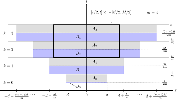
Case I.  We fist assume that $\mu(\mathrm{d}x)={{\rm 1\mkern-1.5mu}\!{\rm I}}_{Q(\ell)}\mathrm{d}x$ for some $\ell>0$. Denote

$$c(m):=\exp\left(-\Theta\>m^{\alpha}[\log(m)]^{1+\alpha}\right),$$ (8.4)

where $\Theta$ is a constant defined in Lemma 8.2. We comment that due to a version mismatch in [8], $B_{0}$ should be defined separately, i.e.,

$$A_{k} :=\left\{u(s,x)\geq\beta^{k+1}{{\rm 1\mkern-1.5mu}\!{\rm I}}_{S_{k}^{m}}(x)\>\text{for all $s\in\left[\frac{(2k+1)t}{2m},\frac{(k+1)t}{m}\right]$ and $x\in\mathbb{R}^{d}$}\right\},\quad k\geq 0,$$

$$B_{k} :=\left\{u(s,x)\geq\beta^{k+1}{{\rm 1\mkern-1.5mu}\!{\rm I}}_{S_{k}^{m}}(x)\>\text{for all $s\in\left[\frac{kt}{m},\frac{(2k+1)t}{2m}\right]$ and $x\in\mathbb{R}^{d}$}\right\},\quad k\geq 1,$$

$$B_{0} :=\left\{u\left(\frac{t}{2m},x\right)\geq\beta{{\rm 1\mkern-1.5mu}\!{\rm I}}_{S_{0}^{m}}(x)\>\text{for all $x\in\mathbb{R}^{d}$}\right\},$$

where

$$S^{m}_{k}:=\>\left(-\ell-\frac{Mk}{m},\ell+\frac{Mk}{m}\right)\>.$$

See Figure 1 for an illustration of the schema.

Figure 1: Induction schema for the strong comparison principle in the one-spatial dimension case.

By an argument using the strong Markov property, one can show that

$$\mathbb{P}\left(A_{k}\mid\mathcal{F}_{kt/m}\right)\geq 1-c(m),\quad\text{a.s. on $A_{k-1}$ for $0\leq k\leq m-1$,}$$

which implies

$$\mathbb{P}\left(A_{k}\mid A_{k-1}\cap\cdots\cap A_{0}\right)\geq 1-c(m),\quad\text{for all $1\leq k\leq m-1$.}$$

Notice that the fact that $A_{0}\subseteq B_{0}$ implies that $\mathbb{P}(B_{0})\geq\mathbb{P}(A_{0})\geq 1-c(m)$. By similar arguments as those for $A_{k}$, one can show that

$$\mathbb{P}\left(B_{k}\mid B_{k-1}\cap\cdots\cap B_{0}\right)\geq 1-c(m),\quad\text{for all $1\leq k\leq m-1$.}$$

Then,

$$\mathbb{P}\left(\cap_{0\leq k\leq m-1}\left[A_{k}\cap B_{k}\right]\right) \geq 1-\left(1-\mathbb{P}\left(\cap_{0\leq k\leq m-1}A_{k}\right)\right)-\left(1-\mathbb{P}\left(\cap_{0\leq k\leq m-1}B_{k}\right)\right)$$

$$\geq(1-c(m))^{m-1}\mathbb{P}(A_{0})+(1-c(m))^{m-1}\mathbb{P}(B_{0})-1$$

$$\geq 2(1-c(m))^{m}-1.$$ (8.5)

Therefore, for all $t>0$ and $M>0$,

$$\mathbb{P}\Big{(}u(s,x)>0\;\;\text{for all $t/2\leq s\leq t$ and $x\in Q(M/2)$}\Big{)} \geq\lim_{m\rightarrow\infty}\mathbb{P}\Big{(}\cap_{0\leq k\leq m-1}\left[A_{k}\cap B_{k}\right]\Big{)}$$

$$\geq\lim_{m\rightarrow\infty}2(1-c(m))^{m}-1=1.$$

Since $t$ and $M$ are arbitrary, this completes the proof for the case when $\mu(\mathrm{d}x)={{\rm 1\mkern-1.5mu}\!{\rm I}}_{Q(\ell)}\mathrm{d}x$.

Case II.  Now for general initial data $\mu$, we only need to prove that for each $\epsilon>0$,

$$\mathbb{P}\left(u(t,x)>0\;\text{for $t\geq\epsilon$ and $x\in\mathbb{R}^{d}$}\right)=1.$$ (8.6)

Fix $\epsilon>0$. Denote $V(t,x):=u(t+\epsilon,x)$. By the Markov property, $V(t,x)$ solves (1.1) with the time-shifted noise $\dot{M}_{\epsilon}(t,x):=\dot{M}(t+\epsilon,x)$ starting from $V(0,x)=u(\epsilon,x)$, i.e.,

$$V(t,x) =\left(u(\epsilon,\circ)*G(t,\cdot)\right)(x)+\iint_{[0,t]\times\mathbb{R}^{d}}\rho(V(s,y))G(t-s,x-y)M_{\epsilon}(\mathrm{d}s,\mathrm{d}y).$$ (8.7)

We first prove by contradiction that

$$\mathbb{P}\left(u(\epsilon,x)=0,\;\text{for all $x\in\mathbb{R}^{d}$}\right)=0.$$ (8.8)

Notice that by Theorem 1.6, the function $x\mapsto u(t,x)$ is Hölder continuous over $\mathbb{R}^{d}$ a.s. The weak comparison principle (Theorem 1.1) shows that $u(t,x)\geq 0$ a.s. Hence, if (8.8) is not true, then by the Markov property and the strong comparison principle in Case I, at all times $\eta\in[0,\epsilon]$, with some strict positive probability, $u(\eta,x)=0$ for all $x\in\mathbb{R}^{d}$, which contradicts Theorem 1.9 as $\eta$ goes to zero. Therefore, there exists a sample space $\Omega^{\prime}$ with $\mathbb{P}(\Omega^{\prime})=1$ such that for each $\omega\in\Omega^{\prime}$, there exists $x\in\mathbb{R}^{d}$ such that $u(\epsilon,x,\omega)>0$.

Since $u(\epsilon,x,\omega)$ is continuous at $x$, one can find two nonnegative constants $c=c(\omega)$ and $\beta=\beta(\omega)$ such that $u(\epsilon,y,\omega)\geq\beta{{\rm 1\mkern-1.5mu}\!{\rm I}}_{x+Q(c)}(y)$ for all $y\in\mathbb{R}^{d}$. Then Case I implies that

$$\mathbb{P}\left(V_{\omega}(t,x)>0\;\text{for all $t\geq 0$ and $x\in\mathbb{R}^{d}$}\right)=1,$$

where $V_{\omega}$ is the solution to (8.7) starting from $u(\epsilon,x,\omega)$. Therefore, (8.6) is true. This completes the proof of Theorem 1.3. ∎

Proof of Theorem 1.4.

Following the proof of Theorem 1.3, since $K$ is compact, we can choose $\eta,T,N>0$ such that $K\subset[\eta,T]\times Q(N)$. Let $\beta$, $A_{k}$ and $B_{k}$ be as in the proof of Theorem 1.3, we have

$$\mathbb{P}\left(\inf_{(t,x)\in K}u(t,x)<\beta^{m}\right)\leq 1-\mathbb{P}\Big{(}\cap_{0\leq k\leq m-1}(A_{k}\cap B_{k})\Big{)}$$

$$\leq 2\left[1-(1-c(m))^{m}\right]\,,$$

where $c(m)$ is a positive quantity defined in (8.4). Then we use the fact that $(1-x)^{m}\geq 1-mx$ for all $x>0$ and $m>1$ to conclude that for some $\Theta^{\prime}$ slightly bigger than the $\Theta$ in (8.4),

$$\mathbb{P}\left(\inf_{(t,x)\in K}u(t,x)<\beta^{m}\right)\leq 2mc(m)\leq\exp\left(-\Theta^{\prime}m^{\alpha}\left(\log m\right)^{1+\alpha}\right)\,.$$

Finally, by taking $m=|\log\epsilon|$, we complete the proof of Theorem 1.4. ∎

Appendix A Appendix: Some technical lemmas

Some technical lemmas are listed in this part.

Lemma A.1.

If $g(t)$ is a monotone function over $[0,T]$, then for all $\beta>0$ and $t\in(0,T]$,

$$\int_{0}^{t}g(t-s)\exp \left(-\frac{2\beta s(t-s)}{t}\right)\mathrm{d}s=\int_{0}^{t}g(s)\exp\left(-\frac{2\beta s(t-s)}{t}\right)\mathrm{d}s$$ (A.1)

$$\leq\begin{cases}\displaystyle 2\int_{0}^{t}g(s)e^{-\beta(t-s)}\mathrm{d}s&\text{if $g$ is nondecreasing,}\\[8.00003pt] \displaystyle 2\int_{0}^{t}g(s)e^{-\beta s}\mathrm{d}s&\text{if $g$ is nonincreasing.}\end{cases}$$ (A.2)

Proof.

Equality (A.1) is clear by change of variables. We first assume that $g(t)$ is nondecreasing in $[0,T]$. Denote the integral by $I$. Then

$$I= \int_{0}^{t/2}g(s)\exp\left(-\frac{2\beta s(t-s)}{t}\right)\mathrm{d}s+\int_{t/2}^{t}g(s)\exp\left(-\frac{2\beta s(t-s)}{t}\right)\mathrm{d}s$$

$$\leq \int_{0}^{t/2}g(s)\exp\left(-\beta s\right)\mathrm{d}s+\int_{t/2}^{t}g(s)\exp\left(-\beta(t-s)\right)\mathrm{d}s$$

$$\leq \int_{t/2}^{t}g(t-s)\exp\left(-\beta(t-s)\right)\mathrm{d}s+\int_{t/2}^{t}g(s)\exp\left(-\beta(t-s)\right)\mathrm{d}s$$

$$\leq 2\int_{t/2}^{t}g(s)\exp\left(-\beta(t-s)\right)\mathrm{d}s$$

$$\leq 2\int_{0}^{t}g(s)\exp\left(-\beta(t-s)\right)\mathrm{d}s.$$

If $g$ is nonincreasing in $[0,T]$, we simply replace the above $g(s)$ by $g(t-s)$ thanks to (A.1). This proves Lemma A.1. ∎

Lemma A.2.

Let $R^{\epsilon}$ be defined in (7.4). If $f$ satisfies (1.4) with $\alpha=1$, then there exists a positive constant $C$ such that for all $0\leq s,\epsilon\leq t$ and $x\in\mathbb{R}^{d}$,

$$\iint_{\mathbb{R}^{2d}}\mathrm{d}y_{1}\mathrm{d}y_{2}\>f(y_{1}-y_{2}) \left(R^{\epsilon}(t-s,\cdot)*G(\epsilon,\cdot)\right)(x-y_{1})$$

$$\times \left(R^{\epsilon}(t-s,\cdot)*G(\epsilon,\cdot)\right)(x-y_{2})\leq C\,.$$

Proof.

Denote the integral by $I$. Using Fourier transform we have

$$I \leq\int_{\mathbb{R}^{d}}e^{-\frac{2(t-s)}{\epsilon}}\sum_{n,m=1}^{\infty}\frac{\left(\frac{t-s}{\epsilon}\right)^{n}}{n!}\frac{\left(\frac{t-s}{\epsilon}\right)^{m}}{m!}e^{-\frac{(n+m)\epsilon}{2}|\xi|^{2}}\hat{f}(\mathrm{d}\xi)$$

$$\leq Ce^{-\frac{2(t-s)}{\epsilon}}\sum_{n,m=1}^{\infty}\left(\frac{t-s}{\epsilon}\right)^{m+n}\frac{1}{n!m!}\,.$$

Letting $n+m=k$ and using the fact that

$$\sum_{n=1}^{k-1}\frac{1}{n!(k-n)!}=\frac{1}{k!}(2^{k}-2)\,,$$

we see that the above double sum is equal to

$$\sum_{k=1}^{\infty}\sum_{n=1}^{k-1}\left(\frac{t-s}{\epsilon}\right)^{k}\frac{1}{n!(k-n)!} \leq\sum_{k=1}^{\infty}\left(\frac{t-s}{\epsilon}\right)^{k}\frac{2^{k}}{k!}\leq e^{\frac{2(t-s)}{\epsilon}}-1\,,$$

which proves Lemma A.2. ∎

Lemma A.3.

There exists a finite constant $C>0$ such that

$$\int_{\mathbb{R}^{d}}|R^{\epsilon}(t,x)-G(t,x)|\mathrm{d}x\leq e^{-t/\epsilon}+C\left(\frac{\epsilon}{t}\right)^{1/2}\,,$$ (A.3)

and

$$\int_{\mathbb{R}^{d}}|G(t+\epsilon,x)-G(t,x)|\mathrm{d}x\leq C\log\left(1+\frac{\epsilon}{t}\right)\,,$$ (A.4)

for all $\epsilon>0$ and $t>0$.

Proof.

Because $\left|\frac{\partial}{\partial t}G(t,x)\right|\leq Ct^{-1}G(2t,x)$, we see that for any $0<t\leq t^{\prime}$,

$$\int_{\mathbb{R}^{d}}|G(t^{\prime},x)-G(t,x)|\mathrm{d}x \leq\int_{\mathbb{R}^{d}}\mathrm{d}x\int_{t}^{t^{\prime}}\mathrm{d}s|\frac{\partial}{\partial s}G(s,x)|$$

$$\leq C\int_{\mathbb{R}^{d}}\mathrm{d}x\int_{t}^{t^{\prime}}\mathrm{d}s\>s^{-1}G(2s,x)$$

$$\leq C\log\left(t^{\prime}/t\right).$$

The rest of the proof will follow exactly the same lines as those in the proof of Lemma 8.2 in [8] and we will not repeat here. ∎

Lemma A.4.

The function $g(t,x):=\int_{0}^{t}(2\pi s)^{-d/2}\exp\left(-\frac{x^{2}}{2s}\right)\mathrm{d}s$, for $t,x\geq 0$, satisfies the following properties,

1. $x\mapsto g(t,x)$ is strictly decreasing functions on $x\in(0,\infty)$.

2. If $d=1$, then $g(t,x)$ doesn’t blow up at $x=0$ and $g(t,x)\leq g(t,0)=\sqrt{2t/\pi}$. If $d\geq 2$, then $g(t,x)$ blows up at $x=0$.

3. If $d=1,2$, then for all $\theta>0$ and $t>0$,

   $$\int_{\mathbb{R}^{d}}g(t,|x|)^{\theta}\mathrm{d}x<\infty.$$ (A.5)

4. If $d\geq 3$, then for all $0<\theta<\frac{d}{d-2}$ and $t>0$, (A.5) holds.

Proof.

(1) It is clear $x\mapsto g(t,x)$ is a nonincreasing function on $(0,\infty)$ because

$$\frac{\partial}{\partial x}g(t,x)=-\int_{0}^{t}(2\pi s)^{-d/2}\frac{x}{s}\exp\left(-\frac{x^{2}}{2s}\right)\mathrm{d}s<0,\quad\text{for $x>0$.}$$

(2) If $d=1$, then by (1), we see that $g(t,x)\leq g(t,0)=\sqrt{2t/\pi}$. By change of variables $z=x^{2}/(2s)$,

$$g(t,x)=\frac{1}{2\pi^{d/2}}x^{2-d}\int_{\frac{x^{2}}{2t}}^{\infty}e^{-z}z^{\frac{d}{2}-2}\mathrm{d}z.$$ (A.6)

If $d=2$, then the integral in (A.6) blows up as $x\rightarrow 0_{+}$. When $d\geq 3$,

$$g(t,x)\leq\frac{1}{2\pi^{d/2}}x^{2-d}\int_{0}^{\infty}e^{-z}z^{\frac{d}{2}-2}\mathrm{d}z=\frac{\Gamma(d/2-1)}{2\pi^{d/2}}x^{2-d},$$ (A.7)

which blows up as $x\rightarrow 0_{+}$.
(3) If $d=1$, for all $t>0$ and $x\geq 0$,

$$g(t,x)\leq \frac{1}{\sqrt{2\pi}}e^{-\frac{x^{2}}{2t}}\int_{0}^{t}\frac{1}{\sqrt{s}}\mathrm{d}s=\frac{\sqrt{2t}}{\sqrt{\pi}}e^{-\frac{x^{2}}{2t}}\,,$$

which shows (A.5) for $d=1$. If $d=2$, then

$$g(t,x)=\frac{1}{2\pi}\int_{x^{2}/(2t)}^{\infty}e^{-z}z^{-1}\mathrm{d}z.$$

Then by l’Hopital’s rule,

$$\lim_{x\rightarrow 0_{+}}\frac{g(t,x)}{\log(1/x)}=\frac{1}{2\pi}\lim_{x\rightarrow 0_{+}}\frac{-e^{-\frac{x^{2}}{2t}}\frac{2t}{x^{2}}\>\frac{x}{t}}{-1/x}=\frac{1}{\pi}.$$

While for $x\geq 1$,

$$g(t,x)= \frac{1}{2\pi}\int_{\frac{x^{2}}{2t}}^{\infty}e^{-z}z^{-\frac{3}{2}}\mathrm{d}z\leq\frac{1}{2\pi}\left(\frac{x^{2}}{2t}\right)^{-\frac{3}{2}}\int_{\frac{x^{2}}{2t}}^{\infty}e^{-z}\mathrm{d}z\leq\frac{(2t)^{3/2}}{2\pi}e^{-\frac{x^{2}}{2t}}\,,$$

from which we can conclude (3).
(4) For $d\geq 3$, note that there is a constant $C_{d}>0$ which only depends on $d$ such that $z^{\frac{d}{2}-2}e^{-z}\leq C_{d}e^{-\frac{z}{2}}$ for all $z\geq 0$. Then for $x\geq 1$,

$$g(t,x)=\frac{1}{2\pi^{d/2}}x^{2-d}\int_{\frac{x^{2}}{2t}}^{\infty}e^{-z}z^{\frac{d}{2}-2}\mathrm{d}z\leq\frac{C_{d}}{2\pi^{d/2}}\int_{\frac{x^{2}}{2t}}^{\infty}e^{-\frac{z}{2}}\mathrm{d}z\leq\frac{C_{d}}{\pi^{d/2}}e^{-\frac{x^{2}}{4t}}\,,$$

this shows that for any $\theta>0$,

$$\int_{|x|\geq 1}g(t,|x|)^{\theta}\mathrm{d}x<\infty\,.$$ (A.8)

The restriction that $\theta<\frac{d}{d-2}$ comes from the integrability on $|x|\leq 1$, which is clear from the upper bound of $g(t,x)$ in (A.7). This completes the proof of Lemma A.4. ∎

Lemma A.5.

Recall the function $g(t,x)$ is defined in Lemma A.4. Let $\psi\in C_{c}(\mathbb{R}^{d})$ be an arbitrary mollifier such that $\int_{\mathbb{R}^{d}}\psi(x)\mathrm{d}x=1$. Denote $\psi_{\epsilon}(x)=\epsilon^{-d}\psi(x/\epsilon)$. For each fixed $t>0$, suppose that $h:\mathbb{R}^{d}\mapsto\mathbb{R}_{+}$ is a nonnegative and measurable function such that

$$\int_{\mathbb{R}^{d}}h(x)g(2t,|x|)\mathrm{d}x<\infty.$$

Then the following statements hold:

1. For any $\eta>0$, there exists $\phi\in C_{c}(\mathbb{R}^{d})$ such that

   $$\sup_{\epsilon\in(0,\sqrt{t})}\int_{\mathbb{R}^{d}}g_{\epsilon}(t,|x|)\left|h(x)-\phi(x)\right|\mathrm{d}x<\eta,$$

   where $g_{\epsilon}(t,|x|)=\int_{\mathbb{R}^{d}}g(t,|y|)\psi_{\epsilon}(x-y)\mathrm{d}y$.

2. By denoting $h_{\epsilon}(x)=(h*\psi_{\epsilon})(x)$, we have that

   $$\lim_{\epsilon\rightarrow 0}\int_{\mathbb{R}^{d}}{g(t,|x|)}\left|h(x)-h_{\epsilon}(x)\right|\mathrm{d}x=0.$$

Proof.

Without loss of generality, we may assume that $t=1$.

(1)  Fix $\eta>0$. It is clear that for some constant $C>0$, we have

$$\psi(x)\leq CG(1,x),\quad\text{for all $x\in\mathbb{R}^{d}$.}$$

Hence, $\psi_{\epsilon}(x)\leq CG(\epsilon^{2},x)$, which implies that

$$g_{\epsilon}(1,|x|) \leq C\int_{\mathbb{R}^{d}}\mathrm{d}y\>G(\epsilon^{2},x-y)\int_{0}^{1}\mathrm{d}s\>G(s,y)$$

$$=C\int_{0}^{1}\mathrm{d}s\>G(s+\epsilon^{2},x)$$

$$=C\int_{\epsilon^{2}}^{1+\epsilon^{2}}\mathrm{d}s\>G(s,x)\leq Cg(2,|x|)\,,$$ (A.9)

where the last inequality is due to the definition of $g(t,x)$ and $\epsilon\in(0,1)$. Since $h$ is nonnegative, it is known that one can find a monotone nondecreasing sequence $\{s_{j}\}$ of simple functions such that $s_{j}(x)\uparrow h(x)$ pointwise; see, e.g., Theorem 1.44 in [1]. Hence,

$$\sup_{\epsilon\in(0,1)}\int_{\mathbb{R}^{d}}g_{\epsilon}(1,|x|)\left|h(x)-s_{j}(x)\right|\mathrm{d}x <C\int_{\mathbb{R}^{d}}g(2,|x|)\left|h(x)-s_{j}(x)\right|\mathrm{d}x\rightarrow\infty$$

as $j\rightarrow\infty$, where the last limit is due to the dominated convergence. Hence, for some $s\in\{s_{j}\}$,

$$\sup_{\epsilon\in(0,1)}\int_{\mathbb{R}^{d}}g_{\epsilon}(1,|x|)\left|h(x)-{s(x)}\right|\mathrm{d}x\leq\eta/2.$$

Now we choose and fix $q>1$ such that

$$C(g,d,q):=\int_{\mathbb{R}^{d}}g(t,|x|)^{q}\mathrm{d}x<\infty\,.$$ (A.10)

This is possible thanks to Lemma A.4: $q>1$ can be any number for $d=1,2$ and $q\in(1,\frac{d}{d-2})$ for $d\geq 3$. Since $s$ is a simple function with bounded support, by Lusin’s theorem (see e.g., Theorem 1.42 (f) in [1]) there exists $\phi\in C_{c}(\mathbb{R}^{d})$ such that

$$|\phi(x)|\leq\left|\left|s\right|\right|_{L^{\infty}(\mathbb{R}^{d})},\quad\text{for all $x\in\mathbb{R}^{d}$}$$

and

$$\text{Vol}\left(\left\{x\in\mathbb{R}^{d}:\>\phi(x)\neq s(x)\right\}\right)\leq\frac{\eta^{p}}{\left(4C\left|\left|s\right|\right|_{L^{\infty}(\mathbb{R}^{d})}C(g,d,q)^{1/q}\right)^{p}}\,,$$

where $1/p+1/q=1$ and $C$ is as in (A.9). Thus, using (A.9) and the Hölder inequality,

$$\sup_{\epsilon\in(0,1)} \int_{\mathbb{R}^{d}}g_{\epsilon}(1,|x|)\left|s(x)-\phi(x)\right|\mathrm{d}x$$

$$\leq C\int_{\mathbb{R}^{d}}g(2,|x|)\left|s(x)-\phi(x)\right|\mathrm{d}x$$

$$\leq 2C\left|\left|s\right|\right|_{L^{\infty}(\mathbb{R}^{d})}\int_{\mathbb{R}^{d}}{{\rm 1\mkern-1.5mu}\!{\rm I}}_{\left\{x\in\mathbb{R}^{d}:\>\phi(x)\neq s(x)\right\}}g(2,|x|)\mathrm{d}x$$

$$\leq 2C\left|\left|s\right|\right|_{L^{\infty}(\mathbb{R}^{d})}\left(\int_{\mathbb{R}^{d}}{{\rm 1\mkern-1.5mu}\!{\rm I}}_{\left\{x\in\mathbb{R}^{d}:\>\phi(x)\neq s(x)\right\}}\mathrm{d}x\right)^{\frac{1}{p}}\left(\int_{\mathbb{R}^{d}}g(2,|x|)^{q}\mathrm{d}x\right)^{\frac{1}{q}}$$

$$\leq\frac{\eta}{2}\,.$$

This completes the proof of (1).

(2)  For any $\eta>0$, we can write

$$\int_{\mathbb{R}^{d}}|h_{\epsilon}(x)-h(x)|g(1,|x|)\mathrm{d}x= \int_{\mathbb{R}^{d}}\left|\int_{\mathbb{R}^{d}}\psi_{\epsilon}(x-y)\left[h(y)-h(x)\right]\mathrm{d}y\right|g(1,|x|)\mathrm{d}x$$

$$= \int_{\mathbb{R}^{d}}\left|\int_{\mathbb{R}^{d}}\psi_{\epsilon}(x-y)\left[h(y)-\phi(y)\right]\mathrm{d}y\right|g(1,|x|)\mathrm{d}x$$

$$+\int_{\mathbb{R}^{d}}\left|\int_{\mathbb{R}^{d}}\psi_{\epsilon}(x-y)\left[\phi(y)-\phi(x)\right]\mathrm{d}y\right|g(1,|x|)\mathrm{d}x$$

$$+\int_{\mathbb{R}^{d}}\left|\int_{\mathbb{R}^{d}}\psi_{\epsilon}(x-y)\left[\phi(x)-h(x)\right]\mathrm{d}y\right|g(1,|x|)\mathrm{d}x$$

$$:= I_{1}+I_{2}+I_{3}\,.$$

For $I_{1}$, choose $\phi\in C_{c}(\mathbb{R}^{d})$ according to (1), such that $I_{1}<\frac{\eta}{3}$. From the proof of (1) it is obvious that with the same choice of $\phi$, $I_{3}<\frac{\eta}{3}$. For $I_{2}$, since $\psi$ is compactly supported, we may choose $\epsilon_{0}>0$ such that whenever $0<\epsilon<\epsilon_{0}$, we have $I_{2}<\frac{\eta}{3}$ because of the uniform continuity of $\phi$. This completes the proof of (2). ∎

Le Chen
Department of Mathematics
University of Kansas
Lawrence, Kansas, 66045-7594
Email: chenle@ku.edu
URL: www.math.ku.edu/u/chenle/

Jingyu Huang
Department of Mathematics
University of Utah
Salt Lake City, UT 84112-0090
Email: jhuang@math.utah.edu
URL: http://www.math.utah.edu/~jhuang/

References

- [1] Adams, Robert A. and John J. F. Fournier. Sobolev spaces (2 ed.). Elsevier/Academic Press, Amsterdam, 2003.
- [2] Balan, Raluca M. and Le Chen Parabolic Anderson model with space-time homogeneous Gaussian noise and rough initial condition Preprint at arXiv:1606.08875, 2016.
- [3] Carmona, René A. and Stanislav A. Molchanov. Parabolic Anderson problem and intermittency. Mem. Amer. Math. Soc., 108 (1994), no. 518, viii+125 pp.
- [4] Chen, Le and Robert C. Dalang. Moments and growth indices for nonlinear stochastic heat equation with rough initial conditions. Ann. Probab. 43 (2015), no. 6, 3006–3051.
- [5] Chen, Le and Robert C. Dalang. Hölder-continuity for the nonlinear stochastic heat equation with rough initial conditions. Stoch. Partial Differ. Equ. Anal. Comput. 2 (2014), no. 3, 316–352.
- [6] Chen, Le, Jingyu Huang, Davar Khoshnevisan and Kunwoo Kim. A badly-behaved parabolic SPDE. In preparation, 2016.
- [7] Chen, Le and Kunwoo Kim. Nonlinear stochastic heat equation driven by spatially colored noise: moments and intermittency. Preprint at arXiv:1510.06046, 2015.
- [8] Chen, Le and Kunwoo Kim. On comparison principle and strict positivity of solutions to the nonlinear stochastic fractional heat equations. Ann. Inst. Henri Poincaré Probab. Stat., to appear (2016).
- [9] Conus, Daniel, Mathew Joseph and Davar Khoshnevisan. Correlation-length bounds, and estimates for intermittent islands in parabolic SPDEs. Electron. J. Probab. 17 (2012), no. 102, 15 pp.
- [10] Dalang, Robert C. Extending the martingale measure stochastic integral with applications to spatially homogeneous s.p.d.e.’s. Electron. J. Probab. 4 (1999), no. 6, 29 pp.
- [11] Dalang, Robert C. and Lluís Quer-Sardanyons. Stochastic integrals for spde’s: a comparison. Expo. Math. 29 (2011), no. 1, 67–109.
- [12] Dawson, Donald A. and Habib Salehi. Spatially homogeneous random evolutions. J. Multivar. Anal. 10 (1980), no. 2, 141–180.
- [13] Flores, G. R. Moreno. On the (strict) positivity of solutions of the stochastic heat equation. Ann. Probab. 42 (2014), no. 4, 1635–1643.
- [14] Foondun, Mohammud and Davar Khoshnevisan. On the stochastic heat equation with spatially-colored random forcing. Trans. Amer. Math. Soc. 365 (2013), no. 1, 409–458.
- [15] Gubinelli, Massimiliano and Nicolas Perkowski. KPZ reloaded. Preprint at arXiv:1508.03877, 2015.
- [16] Hu, Yaozhong, Jingyu Huang and David Nualart. On the intermittency front of stochastic heat equation driven by colored noises. Electron. Commun. Probab. 21 (2016), no. 21, 13 pp.
- [17] Hu, Yaozhong, Jingyu Huang, David Nualart and Samy Tindel. Stochastic heat equations with general multiplicative Gaussian noises: Hölder continuity and intermittency. Electron. J. Probab. 20 (2015), no. 55, 50 pp.
- [18] Huang, Jingyu, Khoa Lê and David Nualart. Large time asymptotics for the parabolic Anderson model driven by spatially correlated noise. Ann. Inst. Henri Poincaré Probab. Stat. to appear, 2016.
- [19] Mueller, Carl. On the support of solutions to the heat equation with noise. Stochastics Stochastics Rep. 37 (1991), no. 4, 225–245.
- [20] Mueller, Carl and David Nualart. Regularity of the density for the stochastic heat equation. Electron. J. Probab., 13 (2008), no. 74, 2248–2258.
- [21] Sanz-Solé, Marta and Mònica Sarrà. Hölder continuity for the stochastic heat equation with spatially correlated noise. Seminar on Stochastic Analysis, Random Fields and Applications, III (Ascona, 1999), 259–268, Progr. Probab., 52, Birkhäuser, Basel, 2002.
- [22] Shiga, Tokuzo. Two contrasting properties of solutions for one-dimensional stochastic partial differential equations. Canad. J. Math. 46 (1994), no. 2, 415–437.
- [23] Tessitore, Gianmario and Jerzy Zabczyk. Strict positivity for stochastic heat equations. Stochastic Process. Appl. 77 (1998), no. 1, 83–98.
- [24] Walsh, John B. An Introduction to Stochastic Partial Differential Equations. In: Ècole d’èté de probabilités de Saint-Flour, XIV—1984, 265–439. Lecture Notes in Math. 1180, Springer, Berlin, 1986.