Quantum many-body theory for electron spin decoherence in nanoscale nuclear spin baths

Abstract

Decoherence of electron spins in nanoscale systems is important to quantum technologies such as quantum information processing and magnetometry. It is also an ideal model problem for studying the crossover between quantum and classical phenomena. At low temperatures or in light-element materials where the spin-orbit coupling is weak, the phonon scattering in nanostructures is less important and the fluctuations of nuclear spins become the dominant decoherence mechanism for electron spins. Since 1950s, semiclassical noise theories have been developed for understanding electron spin decoherence. In spin-based solid-state quantum technologies, the relevant systems are in the nanometer scale and the nuclear spin baths are quantum objects which require a quantum description. Recently, quantum pictures have been established to understand the decoherence and quantum many-body theories have been developed to quantitatively describe this phenomenon. Anomalous quantum effects have been predicted and some have been experimentally confirmed. A systematically truncated cluster correlation expansion theory has been developed to account for the many-body correlations in nanoscale nuclear spin baths that are built up during the electron spin decoherence. The theory has successfully predicted and explained a number of experimental results in a wide range of physical systems. In this review, we will cover these recent progresses. The limitations of the present quantum many-body theories and possible directions for future development will also be discussed.

I Introduction

A quantum object can be in a superposition of states. An isolated quantum object can be in a pure state with full quantum coherence, a state in which each component of the superposition has a deterministic coefficient up to a global phase factor. Quantum coherence gives rise to a series of non-classical phenomena such as interference and entanglement. It is also the basis of quantum technologies Benioff (1980); Feynman (1982); Deutsch (1985), such as quantum cryptography Bennett and Brassard (1984); Gisin et al. (2002), quantum-enhanced imaging and sensing Caves (1981); Budker and Romalis (2007); Giovannetti et al. (2011), and quantum computers DiVincenzo (1995); Ladd et al. (2010).

Realistic quantum systems are always coupled to environments, thus the quantum coherence is destroyed by the environmental noise Leggett et al. (1987); Prokof’ev and Stamp (2000); Zurek (2003). On the one hand, such decoherence processes prevent quantum interference, restore classical behaviors, and pose a critical challenge to quantum technologies. On the other hand, decoherence could be utilized to reveal information about the environments. This prospect has been persued for a long history in magnetic resonance spectroscopy Abragam (1961), where the decoherence of a large number of electronic or nuclear spins are used to reveal the interactions and motions of atoms in bulk materials. In recent years, the progresses in active control and measurement of single spins have allowed single spins to be used as ultrasensitive quantum sensors to reveal the structures and dynamics of the environments with nanoscale resolution Cole and Hollenberg (2009); Zhao et al. (2011a, 2012a) (see Ref. Rondin et al. (2014) for a review).

Additionally, a great diversity of physical systems have been proposed for spin-based quantum technologies and quantum sensing. In particular, the spins of individual electrons and atomic nuclei offer a promising combination of environmental isolation and controllability, thus they can serve as the basic units of quantum machines: the qubits. Electronic and nuclear spins in semiconductors have distinct technical advantages such as scalability and compatability with modern semiconductor technology Moore (1965), tunable spin properties by energy band and wavefunction engineering, and the ability to manipulate the spins by using the well established electron spin resonance and nuclear magnetic resonance techniques as well as optical and electrical approaches Hanson and Awschalom (2008). Here we concentrate on semiconductor quantum dots (QDs) Hanson et al. (2007) and impurity/defect centers such as phosphorus and bismuth donors in silicon Morton et al. (2011) and nitrogen-vacancy (NV) centers in diamond Awschalom et al. (2007). In these nanoscale systems, a few electronic or nuclear spins (referred to as central spins for clarity) can be addressed, so they are used as qubits, while the many unresolved nuclear spins form a magnetic environment that causes decoherence of the central spins. In addition, the central spins are directly coupled to nearby electronic spins from impurities and defects and are also influenced by charge and voltage fluctuations (e.g., from lattice vibration and nearby electron/hole gases and trapped charges) via spin-orbit coupling. However, these environmental noises can be suppressed, e.g., by careful material and device engineering to remove parasitic charge and spin defects, lowering the temperature to suppress phonon scattering, or using light-element materials to suppress the spin-orbit coupling. Therefore, the most relevant noise sources for the central spins in quantum technologies are the nuclear spins.

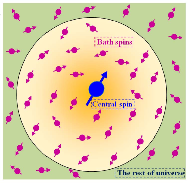
Figure 1: A central spin and the nanoscale spin bath evolve as a closed system in the relevant timescales. The thermal distribution of the spin bath causes a static thermal noise, and the quantum evolution of the spin bath induces a dynamical quantum noise. The rest of universe indicates the larger environment beyond the spin bath, which induces classical noises (being static or dynamical).

Since 1950s, the semiclassical picture of spectral diffusion has been adopted to study the central spin decoherence in spin bathsAnderson and Weiss (1953); Anderson (1954); Kubo (1954). The semiclassical theory treats the spin bath as a source of classical magnetic noise. In modern quantum nanodevices, the wave function of the central spin is localized, so the nuclear spins coupled to the central spin form a nanoscale spin bath. The central spin and the nanoscale spin bath form a closed system in the time scale of interest (see Fig. 1) and the quantum nature of the spin bath becomes important. In recent years, quantum pictures have been established to understand the central spin decoherence. By the quantum theory, anomalous quantum effects have been predicted, some of which have been experimentally confirmed. To quantitatively describe central spin decoherence, a variety of quantum many-body theories have been developed, including the pair-correlation approximation Yao et al. (2006); Liu et al. (2007); Yao et al. (2007), cluster expansion Witzel et al. (2005); Witzel and Das Sarma (2006), linked-cluster expansion Saikin et al. (2007), cluster-correlation expansion (CCE) Yang and Liu (2008a); Yang et al. (2009), disjoint cluster approximation Maze et al. (2008a); Hall et al. (2014), and ring diagram approximation Cywiński et al. (2009a, b). In particular, the CCE theory Yang and Liu (2008a); Yang et al. (2009) provides a systematic account for the many-body correlations in nanoscale spin baths that lead to central spin decoherence. The CCE method has successfully predicted and explained a number of experimental results in a wide range of solid state systems. In this review, we will provide a pedagogical review on the basic concepts of coherence and decoherence, the recent quantum many-body theories, their relationships, limitations, and possible directions for future development.

The organization of this review is as follows. In the first three sections, we introduce the basic concepts (Sec. II), decoherence theory (Sec. III) and coherence protection (Sec. IV) based on the semi-classical noise model. Then we introduce, in Sec. V, the concept of quantum noise and, in Sec. VI, a full quantum picture of central spin decoherence. In Sec. VII, we introduce the coupling of the central spin to the phonon and nuclear spin baths and experimental measurements in paradigmatic solid-state physical systems that identifies the nuclear spin bath as the most relevant decohering environment. Next we review the microscopic quantum many-body theories for central spin decoherence in nuclear spin baths (Sec. VIII) and discuss a series of quantum decoherence effects (Sec. IX). Finally, the possible directions for future development are discussed in Sec. X. For convenience, we take $\hbar=1$ throughout this review.

II Basic concepts of spin decoherence

In this section, we introduce the basic concepts for the environmental noise induced decoherence of a central spin-1/2, including quantum coherence and decoherence, density matrix and ensembles, classification of central spin decoherence and their geometric representation with Bloch vectors, and description of central spin decoherence caused by the simplest environmental noises: rapidly fluctuating noise and static noise.

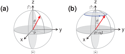
Figure 2: A central spin quantized in a magnetic field along the $z$ axis: (a) geometric representation of a general pure state as a Bloch vector, and (b) central spin evolution as the precession of the Bloch vector around the magnetic field.

Under an external magnetic field, the central spin is quantized along the magnetic field (defined as the $z$ axis) and its evolution is governed by the Zeeman Hamiltonian

$$\hat{H}_{0}=\omega_{0}\hat{S}_{z},$$ (1)

with two energy eigenstates $|\uparrow\rangle$ (spin up) and $|\downarrow\rangle$ (spin down). A general pure superposition state of a spin-1/2 can be parametrized by two real numbers $\theta$ and $\varphi$ as

$$|\theta,\varphi\rangle\equiv\cos\frac{\theta}{2}|\uparrow\rangle+\sin\frac{\theta}{2}e^{i\varphi}|\downarrow\rangle.$$ (2)

Quantum coherence is fully preserved when the central spin is isolated from the environment and undergoes unitary evolution according to its own, deterministic Hamiltonian. For example, the Zeeman Hamiltonian in Eq. (1) leads to the coherent evolution $|\theta,\varphi\rangle\rightarrow e^{-i\hat{H}_{0}t}|\theta,\varphi\rangle=|\theta,\varphi+\omega_{0}t\rangle$. The couplings of the central spin to the environment amounts to measurement of the central spin by the environment (with the results unknown to any observers though). As a result, the central spin undergoes random collapses from a fully coherent pure state into an incoherent mixture (i.e., a statistical ensemble) of distinct pure states, i.e., quantum coherence breaking or decoherence in short.

II.1 Temporal ensembles and spatial ensembles

A quantum system in a pure state $|\psi\rangle$ is described by the density operator $\hat{\rho}=|\psi\rangle\langle\psi|$, while a quantum system that is found in the $k$th distinct pure state $|\psi_{k}\rangle$ with probability $p_{k}$ ($k=1,2,\cdots$) is described by the density operator $\hat{\rho}=\sum_{k}p_{k}|\psi_{k}\rangle\langle\psi_{k}|$. In the energy eigenstates $|\uparrow\rangle$ and $|\downarrow\rangle$ of the central spin, the density operator becomes a 2$\times$2 density matrix as

$$\hat{\rho}=\begin{bmatrix}\rho_{\uparrow\uparrow}&\rho_{\uparrow\downarrow}\\ \rho_{\downarrow\uparrow}&\rho_{\downarrow\downarrow}\end{bmatrix},$$

where the diagonal matrix elements $\rho_{\uparrow\uparrow}$ and $\rho_{\downarrow\downarrow}$ describe the population of each energy eigenstate, and the off-diagonal elements $\rho_{\downarrow\uparrow}=\rho_{\uparrow\downarrow}^{\ast}$ describe the phase correlation between different energy eigenstates.

The density matrix $\hat{\rho}(t)$ describes the statistics of many identical measurements over an ensemble of central spins. In recent years, single-shot measurement of a single central spin has been demonstrated in various solid-state systems Elzerman et al. (2004); Hanson et al. (2005); Barthel et al. (2009); Morello et al. (2010); Neumann et al. (2010); Vamivakas et al. (2010); Robledo et al. (2011); Delteil et al. (2014); Waldherr et al. (2014); Shulman et al. (2014). For such single-spin measurements, one still need to repeat the measurement cycle (i.e., initialization-evolution-measurement) many times to retrieve the correct probabilities of different measurement outcomes. In this case, each cycle corresponds to a sample of the temporal ensemble. According to the characteristic time scale of the noise fluctuation (see Sec. III.1.2 for more details), the environmental noises fall into two categories: dynamical quantum noises that change randomly during the evolution of each sample and static thermal noises that remain invariant for each sample but change randomly from sample to sample (see Sec. V for discussions about the difference between dynamical quantum noises and static thermal noises). Note that “noises” that remain invariant during all repeated measurements just renormalize the external field and do not cause decoherence, e.g., decoherence is suppressed under fast measurements Barthel et al. (2009); Shulman et al. (2014); Delbecq et al. (2016).

In traditional spin resonance measurements, a large number of spatially separated central spins are simultaneously prepared, evolved, and measured. In this case, each central spin is a sample of the spatial ensemble. Since spatially separated spins may be subjected to different static macroscopic conditions (e.g., due to inhomogeneous magnetic fields, $g$-factors, and strains), this introduces additional static noises that could qualitatively change the central spin dephasing Dobrovitski et al. (2008). Nevertheless, since static noises are just static inhomogeneities of the environments for different samples, they can be eliminated by techniques that remove these inhomogeneities, such as spin echo Hahn (1950); Jelezko et al. (2004a). It is also possible to employ environmental engineering to suppress quasi-static noises. For example, to combat electron spin decoherence in nuclear spin baths, a widely pursued approach is to narrow the distribution of the quasi-static noise by polarizing the bath Coish and Loss (2004); London et al. (2013); Liu et al. (2014), quantum measurements of the bath Giedke et al. (2006); Klauser et al. (2006); Stepanenko et al. (2006); Cappellaro (2012); Shulman et al. (2014), and nonlinear feedback between the electron spins and the nuclear spin baths Greilich et al. (2007); Xu et al. (2009); Sun et al. (2012); Latta et al. (2009); Bluhm et al. (2010); Togan et al. (2011) (see Ref. Yang and Sham (2013) for the theories about the nonlinear feedback). Thus the dynamical quantum noises are the most relevant mechanism of central spin dephasing. Single-spin and many-spin measurements would give similar statistics if the dynamical quantum noise do not vary appreciably for spatially separated spins.

II.2 Classification of decoherence processes

The state of the central spin can be visualized by the Bloch vector defined as $2\langle\hat{\mathbf{S}}(t)\rangle\equiv 2\operatorname*{Tr}[\hat{\mathbf{S}}\hat{\rho}(t)]$ through the decomposition

$$\hat{\rho}(t)=\frac{\hat{I}}{2}+\langle\hat{\mathbf{S}}(t)\rangle\cdot\hat{\boldsymbol{\sigma}},$$

where $\hat{I}$ is the identity matrix and $\hat{\boldsymbol{\sigma}}=(\hat{\sigma}_{x},\hat{\sigma}_{y},\hat{\sigma}_{z})^{T}$ are Pauli matrices along the $x/y/z$ directions. The Bloch vector of the general pure state $|\theta,\varphi\rangle$ in Eq. (2) is a unit vector with polar angle $\theta$ and azimuth angle $\varphi$ [Fig. 2(a)]. The unitary evolution transforms a pure state into another pure state with the length of the Bloch vector preserved. For example, the coherent evolution $|\theta,\varphi\rangle\rightarrow|\theta,\varphi+\omega_{0}t\rangle$ governed by the Zeeman Hamiltonian in Eq. (1) is mapped to the Larmor precession of the Bloch vector around the magnetic field ($z$ axis) [Fig. 2(b)]: $\langle\mathbf{\dot{S}}(t)\rangle=\omega_{0}\mathbf{e}_{z}\times\langle\hat{\mathbf{S}}(t)\rangle$ or equivalently $\langle\dot{S}_{z}(t)\rangle=0$ and $\langle\dot{S}_{-}(t)\rangle=-i\omega_{0}\langle\hat{S}_{-}(t)\rangle$, where $S_{\pm}\equiv S_{x}\pm iS_{y}$. By contrast, spin decoherence transforms, via non-unitary evolution, a pure state into a mixed state, described by a Bloch vector with shrinking length.

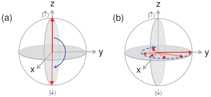
Figure 3: Evolution of the Bloch vector under (a) spin relaxation and (b) spin dephasing.

The environmental noise induces two kinds of changes to the central spin state:

1. Spin relaxation (also called longitudinal relaxation or $T_{1}$ process in literature), which refers to the change of the diagonal populations $\rho_{\uparrow\uparrow}(t)$ and $\rho_{\downarrow\downarrow}(t)$ or equivalently the longitudinal component of the Bloch vector $2\langle\hat{S}_{z}(t)\rangle=\rho_{\uparrow\uparrow}(t)-\rho_{\downarrow\downarrow}(t)$, as shown in Fig. 3(a).

2. Spin dephasing (also called transverse relaxation or $T_{2}$ process in literature), which refers to the decay of the off-diagonal coherence

   $$L(t)\equiv\frac{\rho_{\uparrow\downarrow}(t)}{\rho_{\uparrow\downarrow}(0)}=\frac{\langle\hat{S}_{-}(t)\rangle}{\langle\hat{S}_{-}(0)\rangle}$$ (3)

   or equivalently the transverse components $\langle\hat{S}_{x}(t)\rangle=\operatorname{Re}\rho_{\uparrow\downarrow}(t)$ and $\langle\hat{S}_{y}(t)\rangle=-\operatorname{Im}\rho_{\uparrow\downarrow}(t)$ of the Bloch vector, as shown in Fig. 3(b).

The spin relaxation ($T_{1}$ process) is always accompanied by spin dephasing ($T_{2}$ process), but there are two kinds of physical mechanisms that contribute to pure dephasing (i.e., without causing spin relaxation): (1) dynamical quantum noises lead to “true” decoherence $(T_{\varphi}$ process) Joos et al. (2003); (2) static thermal noises lead to inhomogeneous dephasing ($T_{2}^{\ast}$ process). For $T_{1}$ and $T_{\varphi}$ processes, to provide an intuitive physical picture, we only consider noises that flucutate and hence lose memory much faster than central spin decoherence.

II.3 Spin relaxation (T₁ process)

When the environmental noise induces the central spin flip between $|\uparrow\rangle$ and $|\downarrow\rangle$, the central spin energy changes by an amount $\omega_{0}$, which is compensated by the environment to ensure the conservation of energy. For noises that fluctuate rapidly and hence lose memory much faster than the central spin relaxes, the random central spin flip is memoryless, i.e., the central spin state at time $t$ completely determines its state at the next instant. If $\hat{\rho}(t)=|\psi\rangle\langle\psi|$ is a pure superposition $|\psi\rangle\equiv|\psi_{\uparrow}\rangle+|\psi_{\downarrow}\rangle$ of the spin-up component $|\psi_{\uparrow}\rangle$ and spin-down component $|\psi_{\downarrow}\rangle$ and the environment induces the random jump $|\uparrow\rangle\rightarrow|\downarrow\rangle$ at a constant rate $\gamma$ [Fig. 3(a)], then during a small interval $dt$, the component $|\psi_{\downarrow}\rangle$ remains intact, while $|\psi_{\uparrow}\rangle$ has a probability $\gamma dt$ to incoherently jump to $\hat{S}_{-}|\psi_{\uparrow}\rangle=\hat{S}_{-}|\psi\rangle$. Therefore, the central spin state at the next instant $t+dt$ is given by the density matrix

$$\hat{\rho}(t+dt)=\hat{M}_{1}\hat{\rho}(t)\hat{M}_{1}^{\dagger}+\hat{M}_{0}\hat{\rho}(t)\hat{M}_{0}^{\dagger},$$

which describes the incoherent mixture of the collapsed component $\sqrt{\gamma dt}\hat{S}_{-}|\psi\rangle\equiv\hat{M}_{1}|\psi\rangle$ and the non-collapsed component

$$|\psi_{\downarrow}\rangle+\sqrt{1-\gamma dt}|\psi_{\uparrow}\rangle\approx e^{-(\gamma dt/2)\hat{S}_{-}^{\dagger}\hat{S}_{-}}|\psi\rangle\equiv\hat{M}_{0}|\psi\rangle.$$

This evolution corresponds to a general binary-outcome weak measurement of the central spin by the environment (with the results unknown to any observers): depending on the two possible outcomes, the central spin collapses to $\hat{M}_{1}|\psi\rangle$ or $\hat{M}_{0}|\psi\rangle$. The central spin evolution due to the random jump $|\uparrow\rangle\rightarrow|\downarrow\rangle$ is

$$[\dot{\rho}(t)]_{|\uparrow\rangle\rightarrow|\downarrow\rangle}\equiv\frac{\hat{\rho}(t+dt)-\hat{\rho}(t)}{dt}=\gamma\mathcal{D}[\hat{S}_{-}]\hat{\rho}(t),$$

where $\mathcal{D}[\hat{L}]\hat{\rho}\equiv\hat{L}\hat{\rho}\hat{L}^{\dagger}-\{\hat{L}^{\dagger}\hat{L},\hat{\rho}\}/2$ is the standard Lindblad form for dissipation.

In general, an environment could not only induce $|\uparrow\rangle\rightarrow|\downarrow\rangle$ by absorbing an energy quantum $\omega_{0}$ from the central spin, but also induce the reverse process $|\downarrow\rangle\rightarrow|\uparrow\rangle$ by delivering an energy quantum $\omega_{0}$ to the central spin. When the environment is in thermal equilibrium with an inverse temperature $\beta\equiv 1/(k_{B}T_{\mathrm{env}})$, the latter process would be slower than the former process by a Boltzman factor $e^{-\beta\omega_{0}}$, e.g., for $T_{\mathrm{env}}=0$, the environment is in its ground state and hence cannot deliver the energy quantum $\omega_{0}$, so the latter process is blocked. Including both processes, the environment induced central spin evolution is described by

$$[\dot{\rho}(t)]_{\mathrm{T}_{1}}=\gamma(\mathcal{D}[\hat{S}_{-}]+e^{-\beta\omega_{0}}\mathcal{D}[\hat{S}_{+}])\hat{\rho}(t)=\begin{bmatrix}-\frac{\rho_{\uparrow\uparrow}(t)-\rho_{\uparrow\uparrow}^{\mathrm{eq}}}{T_{1}}&-\frac{\rho_{\uparrow\downarrow}(t)}{2T_{1}}\\ -\frac{\rho_{\downarrow\uparrow}(t)}{2T_{1}}&-\frac{\rho_{\downarrow\downarrow}(t)-\rho_{\downarrow\downarrow}^{\mathrm{eq}}}{T_{1}}\end{bmatrix},$$ (4)

which is characterized by a single time constant $T_{1}\equiv[(1+e^{\beta\omega_{0}})\gamma]^{-1}$ (so-called spin relaxation time) and drives the central spin into thermal equilibrium with the environment:

$$\hat{\rho}^{\mathrm{eq}}\equiv\frac{e^{-\beta\hat{H}_{0}}}{\operatorname*{Tr}e^{-\beta\hat{H}_{0}}}=\begin{bmatrix}\frac{1}{1+e^{\beta\omega_{0}}}&0\\ 0&\frac{e^{\beta\omega_{0}}}{1+e^{\beta\omega_{0}}}\end{bmatrix}.$$

During the spin relaxation process, both the populations and the off-diagonal coherence of the central spin exponentially decay to their respective thermal equilibrium values, with the decay rate of the latter being only half that of the former.

II.4 “True” decoherence by dynamical quantum noises ($T_{\varphi}$ process)

During pure dephasing, the environmental noise induces random jumps of the relative phase between the energy eigenstates $|\uparrow\rangle$ and $|\downarrow\rangle$ of the central spin. For noises that lose memory much faster than the spin dephasing, the central spin evolution is memoryless. Again we take $\hat{\rho}(t)=|\psi\rangle\langle\psi|$ and assume that the environment induces the random phase jump $|\psi\rangle\rightarrow\hat{\sigma}_{z}|\psi\rangle$ at a constant rate $\gamma_{\varphi}$. The central spin state at the next instant $t+dt$ is an incoherent mixture of $\sqrt{\gamma_{\varphi}dt}\hat{\sigma}_{z}|\psi\rangle\equiv\hat{M}_{\mathrm{c}}|\psi\rangle$ and

$$\sqrt{1-\gamma_{\varphi}dt}|\psi\rangle\approx e^{-(\gamma_{\varphi}dt/2)\hat{\sigma}_{z}^{\dagger}\hat{\sigma}_{z}}|\psi\rangle\equiv\hat{M}_{\mathrm{nc}}|\psi\rangle,$$

described by the density matrix $\hat{\rho}(t+dt)=\hat{M}_{\mathrm{c}}\hat{\rho}(t)\hat{M}_{\mathrm{c}}^{\dagger}+\hat{M}_{\mathrm{nc}}\hat{\rho}(t)\hat{M}_{\mathrm{nc}}^{\dagger}$. This incoherent collapse corresponds to a general binary-outcome weak measurement of the central spin by the environment (with the results unknown to any observers). The central spin evolution due to this process assumes the standard Lindblad form

$$[\dot{\rho}(t)]_{\mathrm{T}_{\varphi}}=\gamma_{\varphi}\mathcal{D}[\hat{\sigma}_{z}]\hat{\rho}(t)=\begin{bmatrix}0&-\frac{\rho_{\uparrow\downarrow}(t)}{T_{\varphi}}\\ -\frac{\rho_{\downarrow\uparrow}(t)}{T_{\varphi}}&0\end{bmatrix},$$ (5)

which is characterized by a single time constant $T_{\varphi}\equiv 1/(2\gamma_{\varphi})$ (so-called pure dephasing time). During “true” decoherence, the longitudinal Bloch vector component remain invariant, while the magnitude of the transverse components decay exponentially on a time scale $T_{\varphi}$ [Fig. 3(b)].

II.5 Inhomogeneous dephasing by static thermal noises ($T_{2}^{\ast}$ process)

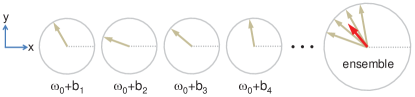
Figure 4: Geometric representation of inhomogeneous dephasing due to averaging over an ensemble of coherently precessing samples.

In the presence of static noises, the central spin evolution is governed by the Hamiltonian $\hat{H}_{\mathbf{b}}\equiv\hat{H}_{0}+\mathbf{\tilde{b}}\cdot\hat{\mathbf{S}}$, where the local field $\mathbf{\tilde{b}}$ remains static for each sample of the ensemble but fluctuates from sample to sample according to a certain probability distribution $P_{\mathrm{inh}}(\mathbf{b})$. For a sample subjected to the local field $\mathbf{b}$, the central spin undergoes unitary evolution $\hat{\rho}_{\mathbf{b}}(t)=e^{-i\hat{H}_{\mathbf{b}}t}\hat{\rho}(0)e^{i\hat{H}_{\mathbf{b}}t}$ and its Bloch vector $\langle\hat{\mathbf{S}}(t)\rangle_{\mathbf{b}}\equiv\operatorname*{Tr}[\hat{\mathbf{S}}\hat{\rho}_{\mathbf{b}}(t)]$ undergoes coherent precession $\langle\mathbf{\dot{S}}(t)\rangle_{\mathbf{b}}=(\omega_{0}\mathbf{e}_{z}+\mathbf{b})\times\langle\hat{\mathbf{S}}(t)\rangle_{\mathbf{b}}$ that preserves its length. The density matrix that describes the ensemble,

$$\hat{\rho}(t)=\int\hat{\rho}_{\mathbf{b}}(t)P_{\mathrm{inh}}(\mathbf{b})d\mathbf{b},$$ (6)

and the Bloch vector

$$\langle\hat{\mathbf{S}}(t)\rangle=\int\langle\hat{\mathbf{S}}(t)\rangle_{\mathbf{b}}P_{\mathrm{inh}}(\mathbf{b})d\mathbf{b}.$$

In principle, the inhomogeneous distribution of the local field can result in both spin relaxation and spin dephasing.

When the external field is much stronger than the noise field, the transverse noises $\tilde{b}_{x},\tilde{b}_{y}$ can hardly tilt the precession axis away from the $z$ axis. In this case, the longitudinal spin relaxation is suppressed by the large energy splitting $\omega_{0}$ between the spin-up $|\uparrow\rangle$ and spin-down $|\downarrow\rangle$ eigenstates, and only pure dephasing by the longitudinal noise $\tilde{b}_{z}$ occurs (see Fig. 4): the different precession frequencies of different samples lead to progressive spread out of their azimuth angles $\varphi_{j}(t)=(\omega_{0}+b_{j})t$ and hence decay of the transverse Bloch vector components $\langle\hat{S}_{-}(t)\rangle$. The off-diagonal coherence (the intrinsic phase factor $e^{-i\omega_{0}t}$ removed)

$$L_{\mathrm{inh}}(t)=\int e^{-ibt}P_{\mathrm{inh}}(b)db$$ (7)

decays on a time scale $T_{2}^{\ast}\sim$ inverse of the characteristic width of the static noise distribution $P_{\mathrm{inh}}(b)$. Such decay by classical ensemble averaging over static noises is called inhomogeneous dephasing ($T_{2}^{\ast}$ process). For the commonly encountered Gaussian distribution

$$P_{\mathrm{inh}}(b)=\frac{1}{\sqrt{2\pi}b_{\mathrm{rms}}}e^{-b^{2}/(2b_{\mathrm{rms}}^{2})},$$ (8)

the spin coherence shows the Gaussian decay:

$$L_{\mathrm{inh}}(t) =e^{-(t/T_{2}^{\ast})^{2}},$$ (9a)

$$T_{2}^{\ast} =\frac{\sqrt{2}}{b_{\mathrm{rms}}}.$$ (9b)

As will be discussed in Sec. IV, the $$T_{2}^{\ast}$$ process can be completely removed by spin echo techniques.

II.6 Summary

Including the unitary evolution under the external field [Eq. (1)] and a fixed local field $b$, as well as the $T_{1}$ and $T_{\varphi}$ processes caused by rapidly fluctuating noises that lose memory much faster than central spin decoherence [Eqs. (4) and (5)], the density matrix of the central spin obeys the Lindblad master equation

$$\dot{\rho}_{b}(t)=-i[\hat{H}_{0}+b\hat{S}_{z},\hat{\rho}_{b}(t)]-\begin{bmatrix}\frac{[\hat{\rho}_{b}(t)]_{\uparrow\uparrow}-\rho_{\uparrow\uparrow}^{\mathrm{eq}}}{T_{1}}&\frac{[\hat{\rho}_{b}(t)]_{\uparrow\downarrow}}{T_{2}}\\ \frac{[\hat{\rho}_{b}(t)]_{\downarrow\uparrow}}{T_{2}}&\frac{[\hat{\rho}_{b}(t)]_{\downarrow\downarrow}-\rho_{\downarrow\downarrow}^{\mathrm{eq}}}{T_{1}}\end{bmatrix},$$

where $T_{2}\equiv[1/(2T_{1})+1/T_{\varphi}]^{-1}$ ($\leq 2T_{1}$) is the spin dephasing time. In the presence of inhomogeneous dephasing, the density matrix $\hat{\rho}(t)$ is obtained by averaging $\hat{\rho}_{b}(t)$ over the distribution of $b$. Note that although spin relaxation imposes an upper limit on the spin dephasing time via $T_{2}\leq 2T_{1}$, in typical cases of central spin decoherence $T_{2}$ is much shorter than $T_{1}$ and is limited by pure dephasing ($T_{\varphi}$ and $T_{2}^{\ast}$ processes).

III Semiclassical noise theory for spin decoherence

A simple theoretical treatment of spin decoherence is to describe the environment as a source of classical magnetic noise $\mathbf{\tilde{b}}(t)$ with zero mean $\langle\mathbf{\tilde{b}}(t)\rangle=0$, so the central spin Hamiltonian is

$$\hat{H}(t)=\omega_{0}\hat{S}_{z}+\mathbf{\tilde{b}}(t)\cdot\hat{\mathbf{S}}.$$ (10)

The time-dependent transverse noises $\tilde{b}_{\pm}(t)\equiv\tilde{b}_{x}(t)\pm i\tilde{b}_{y}(t)$ could randomly tilt the precession axis away from the $z$ axis, flip the central spin between the unperturbed eigenstates $|\uparrow\rangle$ and $|\downarrow\rangle$, and hence induce spin relaxation. The longitudinal noise $\tilde{b}_{z}(t)$ randomly modulates the central spin precession frequency along the $z$ axis and induce pure dephasing. Here we consider a strong external magnetic field and hence a large unperturbed precession frequency $\omega_{0}$, so that the noise can be treated as a perturbation.

III.1 Basic concept of classical noise

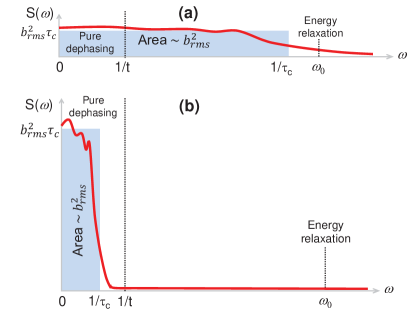
Figure 5: Schematic of the noise spectra for (a) a noise that fluctuates on a time scale $\tau_{c}\ll t$ and (b) a noise that fluctuates on a time scale $\tau_{c}\gtrsim t$, where $t$ is the evolution time.

We take a real, scalar noise $\tilde{b}(t)$ with zero mean $\langle\tilde{b}(t)\rangle=0$ to explain some basic concepts of classical noises. A classical noise is specified by the probability distribution for each realization of the noise, e.g., the probability distribution $P(b_{0},b_{1},\cdots)$ for the noise $\tilde{b}_{n}\equiv\tilde{b}(t_{n})$ at all the time points $t_{n}\equiv n\Delta t$. Below we introduce two important characteristics of noises: statistics and auto-correlations (or equivalently spectra). We will particularly focus on Gaussian noises, which are the simplest and yet a commonly encountered type of noise statistics. Among various noise spectra, we highlight two simple cases, namely, static noises and rapidly fluctuating noises that lose memory much faster than central spin decoherence.

III.1.1 Statistics

According to the form of $P(b_{0},b_{1},\cdots)$, noises are often classified as Gaussian or non-Gaussian. Gaussian noises are one of the simplest and most widely encountered noises. For a Gaussian noise, the random variables $\tilde{b}_{0},\tilde{b}_{1},\cdots$ obey the multivariate normal distribution

$$P(b_{0},b_{1},\cdots)\propto e^{-(1/2)\sum_{ij}b_{i}(\mathbf{C}^{-1})_{ij}b_{j}},$$ (11)

where $\mathbf{C}^{-1}$ is a positive-definite symmetric matrix. In the continuous form, the Gaussian distribution as a functional of the noise $\tilde{b}(t)$ has the form $P[b(t)]\propto e^{(-1/2)\int dt_{1}\int dt_{2}b(t_{1})C^{-1}(t_{1},t_{2})b(t_{2})}$, where $C^{-1}(t_{1},t_{2})$ is a positive-definite symmetric matrix. As a key property, an arbitrary linear combination $\tilde{\varphi}\equiv\sum_{n}c_{n}\tilde{b}_{n}$ of Gaussian random variables is still Gaussian, i.e., still obeys normal distribution. Averaging over Gaussian noises can be obtained explicitly, e.g.,

$$\langle e^{i\tilde{\varphi}}\rangle=e^{-\langle\tilde{\varphi}^{2}\rangle/2},$$ (12)

which can be readily verified by assuming that $\tilde{\varphi}$ obeys Gaussian distribution $P(\varphi)\equiv e^{-\varphi^{2}/(2\sigma^{2})}/(\sqrt{2\pi}\sigma)$. As suggested by Eq. (11), the distribution and hence all moments of the Gaussian noise are completely determined by the matrix $\mathbf{C}$:

$$\langle\tilde{b}_{i}\tilde{b}_{j}\rangle =(\mathbf{C})_{i,j},$$ (13a)

$$\langle\tilde{b}_{i}\tilde{b}_{j}\tilde{b}_{k}\tilde{b}_{l}\rangle =(\mathbf{C})_{i,j}(\mathbf{C})_{k,l}+(\mathbf{C})_{i,k}(\mathbf{C})_{j,l}+(\mathbf{C})_{i,l}(\mathbf{C})_{j,k},$$ (13b)

$$\cdots$$

$$\langle\tilde{b}_{i_{1}}\tilde{b}_{i_{2}}\cdots\tilde{b}_{i_{2M}}\rangle =\sum_{\mathrm{P}}(\mathbf{C})_{i_{p_{1}}i_{p_{2}}}(\mathbf{C})_{i_{p_{3}}i_{p_{4}}}\cdots(\mathbf{C})_{i_{p_{2M-1}}i_{p_{2M}}},$$ (13c)

where $$\sum_{\mathrm{P}} \{i_{1},\cdots,i_{2M}\} \mathbf{C}$$ runs over all possible pairings of . Equation (13) is the Wick’s theorem for Gaussian noises, and Eq. (13a) shows that the matrix in Eq. (11) is the covariance matrix of the Gaussian noise.

III.1.2 Noise auto-correlations

A classical noise is usually characterized by its auto-correlation

$$C(\tau)=\langle\tilde{b}(\tau)\tilde{b}(0)\rangle,$$ (14)

or equivalently the noise spectrum (the power distribution)

$$S(\omega)\equiv\int e^{i\omega\tau}C(\tau)d\tau,$$ (15)

both of which are even functions. The auto-correlation $C(\tau)$ is usually maximal at $\tau=0$ and decays with increasing $|\tau|$. For example, the electron spin bath is usually modelled by the Ornstein-Uhlenbeck noise Dobrovitski et al. (2009); Witzel et al. (2012a, 2014); de Lange et al. (2010), which is Gaussian and has the auto-correlation

$$C(\tau)=b_{\mathrm{rms}}^{2}e^{-|\tau|/\tau_{c}}$$ (16)

and the noise spectrum

$$S(\omega)=2\pi b_{\mathrm{rms}}^{2}\delta^{(1/\tau_{c})}(\omega),$$ (17)

where $\delta^{(\gamma)}(\Delta)\equiv(\gamma/\pi)/(\Delta^{2}+\gamma^{2})$ is the Lorentzian shape function.

The auto-correlation or noise spectrum has three important properties: auto-correlation (or memory) time $\tau_{c}$, the behavior of high-frequency cutoff, and the noise power $b_{\mathrm{rms}}^{2}\equiv\langle\tilde{b}^{2}(0)\rangle=\langle\tilde{b}^{2}(t)\rangle$. The auto-correlation time $\tau_{c}$, which quantifies how fast the noise fluctuates, is the characteristic time for the auto-correlation to decay. Equivalently, $1/\tau_{c}$ is the characteristic cutoff frequency above which the noise spectrum decays significantly [see Eqs. (16) and (17) for the Ornstein-Uhlenbeck noise]. If $\tau_{c}$ is large compared with the achievable time scale of control over the central spin and the high-frequency tail of the spectrum decays faster than power-law decay, then the noise is said to have a hard high-frequency cutoff. Otherwise, the noise has a soft cutoff. For example, the noise spectrum of the Debye phonon bath Uhrig (2007), $S(\omega)=2\alpha\omega\Theta(\omega_{D}-\omega)$ with $\Theta(\omega)$ the Heaviside step function, has a hard cut-off, while that of the Ornstein-Uhlenbeck noise has a soft cutoff as it decays as $1/\omega^{2}$ at high frequency. The noise power is equal to the area of the noise spectrum:

$$b_{\mathrm{rms}}^{2}=\int_{-\infty}^{\infty}S(\omega)\frac{d\omega}{2\pi}=\int_{0}^{\infty}S(\omega)\frac{d\omega}{\pi}.$$

For a fixed noise power, rapidly fluctuating noise has a low and broad spectrum [Fig. 5(a)], while slowly fluctuating noise has a high and narrow spectrum [Fig. 5(b)]. As will be discussed in Sec. III.3, the broad noise spectrum underlies the motional narrowing phenomenon in magnetic resonance spectroscopy Anderson (1954); Abragam (1961).

III.1.3 Markovian and non-Markovian noises and stochastic processes

Considering that there is considerable inconsistency in the terminology of Markovian/non-Markovian stochastic processes, noises, and decoherence, here we would like to make clear our usage of terminology, yet without the intention of unifying the usage in the vast literature. We note that it is useful to distinguish the noise and the stochastic process (such as phonon scattering, atom-atom collisions, and nuclear spin flip-flips) that causes the noise.

A classical noise as the collection of the random variables $\tilde{b}_{n}\equiv\tilde{b}(t_{n})$ at all the time points $t_{n}\equiv n\Delta t$ is characterized by the probability distribution $P(b_{0})$ of $\tilde{b}_{0}$ and the probability distribution $P(b_{n}|b_{0},\cdots,b_{n-1})$ of $\tilde{b}_{n}$ conditioned on $\tilde{b}_{k}$ being $b_{k}$ ($k=0,1,\cdots,n-1)$. The noise is caused by certain microscopic stochastic processes. A stochastic process is called Markovian or memoryless if the distribution of $\tilde{b}_{n}$ depends on $\tilde{b}_{n-1}$ only, i.e., $P(b_{n}|b_{0},\cdots,b_{n-1})=P(b_{n}|b_{n-1})$, so that the probability distribution of the noise can be written as

$$P(b_{0},b_{1},b_{2},\cdots)=P(b_{0})P(b_{1}|b_{0})P(b_{2}|b_{1})\cdots.$$ (18)

Physically, this occurs when the stochastic process (such as a phonon scattering, an atom-atom collision, or a nuclear spin flip-flop) takes a time much shorter than the timescale under consideration. For example, the atom-atom collision is Markovian under the impact approximation, and a phonon scattering is Markovian for a timescale much greater than $\sim$ 1 picosecond. On the other hand, a noise, being caused by either a Markovian or non-Markovian stochastic process, is labeled as Markovian or memoryless when its auto-correlation time $\tau_{c}$ is much shorter than the central spin decoherence time. In general a Markovian or non-Markovian noise could be produced by either a non-Markovian or Markovian stochastic process.

For example, the Ornstein-Uhlenbeck noise [Eqs. (16) and (17)] is caused by the Ornstein-Uhlenbeck process, which is characterized by a Gaussian distribution $P(b_{0})=e^{-b_{0}^{2}/(2b_{\mathrm{rms}}^{2})}/(\sqrt{2\pi}b_{\mathrm{rms}})$ for the initial value $\tilde{b}_{0}$ and a Gaussian conditional distribution for $\tilde{b}_{n}$ Klauder and Anderson (1962):

$$P(b_{n}|b_{n-1},\cdots,b_{0})=P(b_{n}|b_{n-1})=\frac{e^{-(b_{n}-e^{-\Delta t/\tau_{c}}b_{n-1})^{2}/(2\sigma^{2})}}{\sqrt{2\pi}\sigma},$$ (19)

where $\sigma=b_{\mathrm{rms}}\sqrt{1-e^{-2\Delta t/\tau_{c}}}$. Obviously, the Ornstein-Uhlenbeck process is Markovian since the distribution of $\tilde{b}_{n}$ only depends on ${b}_{n-1}$. However, the Ornstein-Uhlenbeck noise has the auto-correlation $\langle\tilde{b}_{n}\tilde{b}_{m}\rangle=b_{\mathrm{rms}}^{2}e^{-|t_{n}-t_{m}|/\tau_{c}}$ [see Eq. (16) for its continuous form], so it could be either Markovian or non-Markovian depending on whether or not its auto-correlation time $\tau_{c}$ is much larger than the central spin decoherence time. In addition, the Ornstein-Uhlenbeck noise is also Gaussian since its distribution function $P(b_{0},b_{1},\cdots)$ can be put into the form of Eq. (11).

Under the classification based on $\tau_{c}$, two kinds of noises are relatively simple: quasistatic noise with $\tau_{c}\gg$ duration of each measurement cycle ($\sim$ central spin decoherence time), and Markovian noise with $\tau_{c}\ll$ duration of each measurement cycle. The static noise $\tilde{b}(t)=\tilde{b}$ is completely specified by its static distribution $P_{\mathrm{inh}}(b)$, so inhomogeneous dephasing caused by static noise can be easily treated (see Sec. II.5). The Markovian noise gives memoryless random jumps of the central spin, as described intuitively in Sec. II.3 (for $T_{1}$ process) and Sec. II.4 (for $T_{\varphi}$ process) in terms of two phenomenological jump rates $\gamma$ and $\gamma_{\varphi}$.

III.2 Spin relaxation by transverse noises

For the sake of simplicity, let us assume $\tilde{b}_{z}(t)=0$. The transverse noise induced central spin flip can be understood in a simple physical picture first proposed by Bloembergen, Purcell, and Pound Bloembergen et al. (1948); Abragam (1961): the fourier spectrum $\tilde{b}_{\pm}(\omega)$ of the transverse noises $\tilde{b}_{\pm}(t)$ may have nonzero components near the unperturbed spin precession frequency $\omega_{0}$ and these components would induce resonant transitions between the two unperturbed eigenstates $|\uparrow\rangle$ and $|\downarrow\rangle$ at a rate proportional to the noise spectrum $S(\omega)\equiv\int\langle\tilde{b}_{-}(\tau)\tilde{b}_{+}(0)\rangle e^{i\omega\tau}d\tau\propto\langle|\tilde{b}_{\pm}(\omega)|^{2}\rangle$ at frequency $\omega_{0}$.

Usually the noise must fluctuate rapidly ($\tau_{c}\lesssim 1/\omega_{0}$) in order for its spectrum to have a significant high frequency component at $\omega_{0}$, so usually $\tau_{c}\ll$ central spin relaxation time ($T_{1}$), i.e., the noise is Markovian. When $\langle\tilde{b}_{-}(t)\tilde{b}_{+}(t^{\prime})\rangle$ is the only nonvanishing noise auto-correlation, the Born-Markovian approximation Abragam (1961) gives the intuitive result [Eq. (4)] for the environment induced central spin evolution, with $\beta=0$ (i.e., the classical noise is equivalent to an environment at infinite temperature) and an explicit expression for the central spin jump rate:

$$\gamma=\frac{1}{2T_{1}}=\frac{S(\omega_{0})}{4},$$

which is the noise spectrum at the central spin transition frequency $\omega_{0}$ (as spin relaxation involves an energy transfer $\omega_{0}$), thus a rapidly fluctuating Markovian noise with $\tau_{c}\lesssim 1/\omega_{0}$ contributes significantly to spin relaxation [Fig. 5(a)], while non-Markovian noises contribute negligibly [Fig. 5(b)].

III.3 Pure dephasing by longitudinal noises

Here we assume $\tilde{b}_{x}(t)=\tilde{b}_{y}(t)=0$ and write $\tilde{b}_{z}(t)$ as $\tilde{b}(t)$ for brevity. In the interaction picture with respect to $\hat{H}_{0}$, the Hamiltonian

$$\hat{H}(t)=\hat{S}_{z}\tilde{b}(t),$$ (20)

describes the random jumps of the central spin transition frequency or equivalently diffusion of the resonance line (similar to Brownian motion). Therefore this model has been known as random frequency modulation or spectral diffusion in the context of magnetic resonance spectroscopy following the pineering work of Anderson Anderson and Weiss (1953); Anderson (1954); Klauder and Anderson (1962) and Kubo Kubo (1954). In the context of quantum computing, this model was elaborated by de Sousa and Das Sarma de Sousa and Das Sarma (2003a, b); de Sousa et al. (2005) to explain the spin echo experiments for donor electron spins in silicon Chiba and Hirai (1972); Tyryshkin et al. (2003); Abe et al. (2004); Ferretti et al. (2005); Tyryshkin et al. (2006). The theory gives reasonable order-of-magnitude agreement (within a factor of 3) for the dephasing time, but fails to explain the $e^{-\tau^{2}}$ decay of the echo envelope de Sousa (2009).

For a general noise, a random relative phase

$$\tilde{\varphi}(t)\equiv\int_{0}^{t}\tilde{b}(t^{\prime})dt^{\prime}$$ (21)

is accumulated between the unperturbed eigenstates $|\uparrow\rangle$ and $|\downarrow\rangle$, leading to the decay of the off-diagonal coherence

$$L(t)=\langle e^{-i\tilde{\varphi}(t)}\rangle.$$ (22)

In contrast to spin relaxation caused by the high frequency part (near $\omega_{0})$ of the noise, the pure dephasing is dominated by low-frequency part of the noise (see Fig. 5), because high frequency components $\omega\gg 1/t$ are effectively averaged out in Eq. (21).

Significant dephasing appears when the root-mean-square phase fluctuation $\sqrt{\langle\tilde{\varphi}^{2}(t)\rangle}$ attains unity, i.e., the dephasing time $T_{2}$ can be estimated from $\langle\tilde{\varphi}^{2}(T_{2})\rangle=1$, where

$$\langle\tilde{\varphi}^{2}(t)\rangle=\int_{0}^{t}dt_{1}\int_{0}^{t}dt_{2}\ \langle\tilde{b}(t_{1})\tilde{b}(t_{2})\rangle.$$ (23)

Here the accumulation of the random phase depends crucially on the ratio between $\tau_{c}$ and $T_{2}$:

1. Quasi-static noise ($\tau_{c}\gg 1/b_{\mathrm{rms}}\sim T_{2}$). Here $\tilde{\varphi}(t)\approx\tilde{b}t$ and hence the phase fluctuation $\sqrt{\langle\tilde{\varphi}^{2}(t)\rangle}\approx b_{\mathrm{rms}}t$ increases linearly with time. This gives inhomogeneous dephasing on a time scale $T_{2}=T_{2}^{\ast}\sim 1/b_{\mathrm{rms}}\ll\tau_{c}$, consistent with the discussion in Sec. II.5. In this regime, the dephasing time is determined only by the noise power and is independent of $\tau_{c}$.

2. Markovian noise ($\tau_{c}\ll 1/b_{\mathrm{rms}}\ll T_{2}$). The noise tends to average out itself during a single measurement cycle, leading to slow, diffusive increase of the phase fluctuation $\sqrt{\langle\tilde{\varphi}^{2}(t)\rangle}\sim(b_{\mathrm{rms}}\tau_{c})\sqrt{t/\tau_{c}}$. This result can also be obtained from Eq. (23) by noting that only $|t_{1}-t_{2}|\lesssim\tau_{c}$ contributes significantly to the integral. This gives “true” decoherence on a time scale $T_{2}=T_{\varphi}\sim 1/(b_{\mathrm{rms}}^{2}\tau_{c})\gg 1/b_{\mathrm{rms}}\gg\tau_{c}$. Actually, the use of Born-Markovian approximation recovers the intuitive result [Eq. (5)] with an explicit expression for the central spin jump rate:

   $$\gamma_{\varphi}=\frac{1}{2T_{\varphi}}=\frac{S(0)}{4}\sim b_{\mathrm{rms}}^{2}\tau_{c}\ll b_{\mathrm{rms}},$$ (24)

   which is the noise spectrum at zero frequency (as pure dephasing involves no energy transfer). The above discussions show that faster fluctuations of the noise lead to longer dephasing time or, in terms of the fourier transform of $L(t)$, narrower magnetic resonance line. This is the motional narrowing phenomenon in magnetic resonance spectroscopy Anderson (1954); Abragam (1961), where the random motion of atoms makes the magnetic noise fluctuate rapidly and hence reduces the width of the magnetic resonance line of the central spin.

On sufficiently short time scales, any noise with a hard high-frequency cutoff becomes static and the small random phase can be treated up to the second order to give Gaussian inhomogeneous dephasing $L_{\mathrm{inh}}(t)=e^{-(b_{\mathrm{rms}}t)^{2}/2}$ [cf. Eq. (9)]. However, the entire dephasing profile over the time scale $\sim T_{2}$ depends on the specific statistics and auto-correlation of the noise.

If the noise is Gaussian, then the dephasing can be obtained from Eq. (12) as Anderson and Weiss (1953)

$$L(t)=e^{-\langle\tilde{\varphi}^{2}(t)\rangle/2}.$$

According to the discussions following Eq. (23), quasi-static noise $(b_{\mathrm{rms}}\tau_{c}\gg 1$) gives Gaussian inhomogeneous dephasing $L_{\mathrm{inh}}(t)=e^{-(t/T_{2}^{\ast})^{2}}$ on a short time scale $T_{2}^{\ast}\sim\sqrt{2}/b_{\mathrm{rms}}\ll\tau_{c}$, consistent with Eq. (9). Markovian noise ($b_{\mathrm{rms}}\tau_{c}\ll 1$) gives exponential “true” decoherence $L(t)=e^{-t/T_{\varphi}}$ on a much longer time scale $T_{\varphi}\sim 1/(b_{\mathrm{rms}}^{2}\tau_{c})\gg\tau_{c}$, consistent with Eq. (24). In the intermediate regime, the dephasing profile depends sensitively on the noise spectrum, e.g., the spectrum of the Ornstein-Uhlenbeck noise in Eqs. (17) gives

$$L(t)=\exp(-b_{\mathrm{rms}}^{2}\tau_{c}t+b_{\mathrm{rms}}^{2}\tau_{c}^{2}(1-e^{-|t|/\tau_{c}})),$$

which reduces to the exponential decoherence with $T_{\varphi}=1/(b_{\mathrm{rms}}^{2}\tau_{c})$ for $t\gg\tau_{c}$ and the Gaussian inhomogeneous dephasing with $T_{2}^{\ast}=\sqrt{2}/b_{\mathrm{rms}}$ for $t\ll\tau_{c}$.

IV Semi-classical noise theory of dynamical decoupling

Dynamical decoupling (DD) is a powerful approach to suppressing the central spin decoherence. The key idea is to dynamically average out the coupling of the central spin to the environment by frequently flipping the central spin. The DD approach originated from the Hahn echo in nuclear magnetic resonance Hahn (1950) and was later developed for high-precision magnetic resonance spectroscopy Mehring (1983); Rhim et al. (1970); Haeberlen (1976). Then the idea of DD was introduced in quantum computing Viola and Lloyd (1998); Ban (1998); Zanardi (1999); Viola et al. (1999), which stimulated numerous studies on applications and extensions to suppressing qubit decoherence for quantum computing (see Ref. Yang et al. (2011) for a review).

DD can efficiently suppress decoherence when the DD induced central spin flip is much faster than the auto-correlation time $\tau_{c}$ of the environmental noise, so that the lost coherence can be retrieved before it is dissipated irreversibly in the environment. According to Sec. III.2, spin relaxation is usually dominated by Markovian noise with $\tau_{c}\lesssim 1/\omega_{0}$, while flipping the central spin usually requires a duration $\gtrsim 1/\omega_{0}$, thus DD is inefficient for suppressing spin relaxation. As discussed in Sec. III.3, pure dephasing is usually dominated by non-Markovian noises and especially static noise, so DD is efficient for combating pure dephasing. Therefore, we only consider pure dephasing in this section.

In a general $N$-pulse DD scheme, the $N$ instantaneous $\pi$-pulses are applied successively at $\tau_{1}<\tau_{2}<\cdots<\tau_{N}$ to induce the flip between $|\uparrow\rangle$ and $|\downarrow\rangle$ and the central spin is measured at a later time $t_{\mathrm{d}}$. In the Schrödinger picture, the central spin Hamiltonian consists of the external field term $\hat{H}_{0}$ [Eq. (1)], the DD control term

$$\hat{H}_{c}(t)=\sum_{n=1}^{N}\pi\delta(t-\tau_{n})\hat{S}_{x},$$ (25)

and the noise term $\tilde{b}(t)\hat{S}_{z}$. A convenient way is to work in the interaction picture with respect to $\hat{H}_{0}+\hat{H}_{c}(t)$, where the central spin Hamiltonian is [cf. Eq. (20)]

$$\hat{H}(t)=s(t)\tilde{b}(t)\hat{S}_{z}$$ (26)

and $s(t)$ is the DD modulation function: it starts from $s(0)=+1$ and changes its sign every time the central spin is flipped by a $\pi$-pulse, i.e., each $\pi$-pulse in the DD switches the sign of the environmental noise. The spin decoherence in the absence of any control is called free-induction decay (FID), which corresponds to a constant modulation function $s(t)\equiv+1$.

Intuitively, when the sign switch by DD is more frequent than the fluctuation of the noise $\tilde{b}(t)$ ($\tau_{c}>$ pulse interval), DD could effectively speed up the noise fluctuation and suppress dephasing efficiently (reminiscent of motional narrowing). On the other hand, when the sign switch coincides with the characteristic fluctuation of a noise, DD could resonantly enhance the effect of the noise $\tilde{b}(t)$, causing rapid decoherence. Below we discuss two important cases: static noises and and Gaussian noises.

If the noise is static during each measurement cycle $[0,t_{\mathrm{d}}]$, then $\tilde{\varphi}(t_{\mathrm{d}})=\tilde{b}\int_{0}^{t_{\mathrm{d}}}s(t)dt$ vanishes when $t_{\mathrm{d}}$ satisfies the echo condition:

$$\int_{0}^{t_{\mathrm{d}}}s(t)dt=0.$$ (27)

This means that a static noise can be completely eliminated at the echo time $t_{\mathrm{d}}$. The simplest DD scheme is Hahn echo Hahn (1950), where a $\pi$-pulse is applied at $\tau$ followed by a measurement at $t_{\mathrm{d}}=2\tau$.

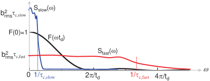
Figure 6: Noise filter for FID and spectra of slowly fluctuating (blue line, $\tau_{c,\mathrm{slow}}\gg t_{\mathrm{d}}$) and fast fluctuating (red line, $\tau_{c,\mathrm{fast}}\ll t_{\mathrm{d}}$) noises.

For Gaussian noises, the central spin dephasing is completely determined by the noise auto-correlation:

$$L(t_{\mathrm{d}})=e^{-\langle\tilde{\varphi}^{2}(t_{\mathrm{d}})\rangle/2},$$ (28)

where Cywinski et al. (2008)

$$\langle\tilde{\varphi}^{2}(t_{\mathrm{d}})\rangle=t_{\mathrm{d}}^{2}\int_{-\infty}^{\infty}S(\omega)F(\omega t_{\mathrm{d}})\frac{d\omega}{2\pi}$$ (29)

is determined by the overlap integral of the noise spectrum $S(\omega)\equiv\int_{-\infty}^{\infty}\langle\tilde{b}(t)\tilde{b}(0)\rangle e^{i\omega t}dt=S(-\omega)$ and the dimensionless noise filter

$$F(\omega t_{\mathrm{d}})\equiv\frac{1}{t_{\mathrm{d}}^{2}}\left|\int_{0}^{t_{\mathrm{d}}}s(t)e^{-i\omega t}dt\right|^{2}=F(-\omega t_{\mathrm{d}}),$$ (30)

which is related to the fourier transform of the DD modulation function $s(t)$ and obeys $F(\omega t_{\mathrm{d}})\leq 1$ as well as the normalization $\int_{-\infty}^{\infty}F(\omega t_{\mathrm{d}})d\omega=2\pi/t_{\mathrm{d}}$.

This noise filter formalism Cywinski et al. (2008) provides a physically transparent undertanding of dephasing caused by Gaussian noise and its control by DD in the frequency domain, e.g., coherence protection can be achieved by designing the noise filter to minimize the overlap integral in Eq. (29).

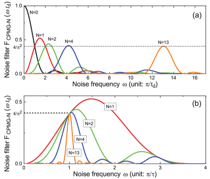
Figure 7: (a) Noise filter functions for FID $(N=0)$ and CPMG-$N$ sequence for fixed total evolution time $t_{\mathrm{d}}$. (b) CPMG-$N$ filter function for fixed pulse interval $\tau$.

For FID, the filter

$$F_{\mathrm{FID}}(\omega t_{\mathrm{d}})=\frac{\sin^{2}(\omega t_{\mathrm{d}}/2)}{(\omega t_{\mathrm{d}}/2)^{2}}\equiv\operatorname{sinc}^{2}\frac{\omega t_{\mathrm{d}}}{2}$$ (31)

passes low-frequency noises ($\omega\lesssim\pi/t_{\mathrm{d}}$) but attenuates high frequency noises ($\omega\gtrsim\pi/t_{\mathrm{d}}$) (black solid line in Fig. 6), i.e., low frequency noises are most effective in causing pure dephasing. For quasi-static noise ($\tau_{c}\gg t_{\mathrm{d}}$), the noise spectrum (blue line in Fig. 6) is well within the low-pass regime of the filter (black line in Fig. 6), so all noise power passes, leading to rapid inhomogeneous dephasing [Eq. (9)]. For Markovian noise ($\tau_{c}\ll t_{\mathrm{d}}$), the noise spectrum is broad (red line in Fig. 6) and remains nearly a constant $S(\omega)\approx\bar{S}\sim b_{\mathrm{rms}}^{2}\tau_{c}$ within the low-pass regime, so $\langle\tilde{\varphi}^{2}(t_{\mathrm{d}})\rangle\approx\bar{S}t_{\mathrm{d}}$ leads to exponential dephasing on a time scale $\sim 1/\bar{S}\sim 1/(b_{\mathrm{rms}}^{2}\tau_{c})$ $\gg$ inhomogeneous dephasing time.

A particularly interesting DD sequence is the $N$-pulse Carr$-$Purcell$-$Meiboom$-$Gill (CPMG-$N$) Carr and Purcell (1954); Meiboom and Gill (1958) consisting of $N$ instantaneous $\pi$-pulses applied at $\tau_{n}=t_{\mathrm{d}}(n-1/2)/N$ $(n=1,2,\cdots,N)$, respectively. The filter for CPMG-$N$ control is

$$F_{\mathrm{CPMG-N}}(\omega t_{\mathrm{d}})=2\frac{\sin^{4}\frac{\omega t_{\mathrm{d}}}{4N}}{\cos^{2}\frac{\omega t_{\mathrm{d}}}{2N}}\frac{1\mp\cos(\omega t_{\mathrm{d}})}{(\omega t_{\mathrm{d}}/2)^{2}}$$

(upper sign for even $N$ and lower sign for odd $N$), which, for $N\gg 1$, has a primary peak at $\omega=N\pi/t_{\mathrm{d}}=\pi/\tau$ ($\tau\equiv t_{\mathrm{d}}/N$ is the pulse interval$)$ and a bandwidth $\sim\pi/t_{\mathrm{d}}$ (see Fig. 7). Near this peak,

$$F_{\mathrm{CPMG-N}}(\omega t_{\mathrm{d}})\approx\frac{4}{\pi^{2}}e^{-t_{\mathrm{d}}^{2}(\omega-N\pi/t_{\mathrm{d}})^{2}/12}=\frac{4}{\pi^{2}}e^{-N^{2}\tau^{2}(\omega-\pi/\tau)^{2}/12}.$$

As mentioned before, for the DD to be efficient, the pulses must be applied faster than the noise auto-correlation time ($\tau<\tau_{c}$). For CPMG-$N$, this is equivalent to that the filter’s peak frequency $\pi/\tau>$ noise cutoff frequency $1/\tau_{c}$. For Markovian noise with $\tau_{c}\ll\tau$, the noise spectrum is nearly constant over the entire band-pass window of the filter, so DD has no effect.

V Quantum noise versus classical noise

In the semiclassical theory of central spin decoherence, the central spin is treated as a quantum object, while the spin bath is approximated by a classical noise. In spin-based solid-state quantum technologies, the nanoscale spin bath is also a quantum object and requires a quantum description. Within the characteristic time scale of central spin decoherence, the central spin and the spin bath can be regarded as a closed quantum system (see Fig. 1). Here we are only interested in the most relevant mechanism for electron spin decoherence in nuclear spin baths: pure dephasing, i.e., we assume that the central spin transition frequency $\omega_{0}$ is far beyond the high-frequency cutoff of the bath noise spectrum. In this case, the central spin and the bath are described by a general pure dephasing Hamiltonian Yao et al. (2006); Liu et al. (2007); Yao et al. (2007)

$$\hat{H}=\hat{H}_{B}+\hat{b}\hat{S}_{z}$$ (32)

in the interaction picture with respect to $\hat{H}_{0}$ [Eq. (1)], where $\hat{H}_{B}$ is the bath Hamiltonian and $\hat{b}$ is the bath noise operator coupled to the central spin.

Below we will classify the noises from the spin bath into two categories according to their natures, namely, static thermal noises and dynamical quantum noises. It should be noted that the noises from the “rest of universe” (Fig. 1), which is taken as classical, can be static or dynamical. Ultimately, all noises have a quantum origin (e.g., the thermal distribution of a spin bath can be ascribed to entanglement between the bath and the rest of universe). Here the static thermal noise and the dynamical quantum noise are differentiated in the sense that the spin bath and the central spin are regarded as a closed quantum system in the timescale of interest.

V.1 Static thermal noises

The initial state of the bath is the maximally mixed thermal state (relevant for nuclear spin baths):

$$\hat{\rho}_{B}^{\mathrm{eq}}=\frac{\hat{I}}{\operatorname*{Tr}\hat{I}}=\sum_{J}P_{J}|J\rangle\langle J|,$$ (33)

When $[\hat{b},\hat{H}_{B}]=0$, $\{|J\rangle\}$ can be chosen as the common eigenstates of $\hat{b}$ and $\hat{H}_{B}$. If the initial state of the bath were a pure state $|J\rangle$, then it would remain in $|J\rangle$, and during the measurement cycle the central spin would evolve under a constant noise field $b_{J}=\langle J|\hat{b}|J\rangle$ from $\hat{\rho}(0)$ to $\hat{\rho}_{J}(t)\equiv e^{-ib_{J}\hat{S}_{z}t}\hat{\rho}(0)e^{ib_{J}\hat{S}_{z}t}$ with an oscillating off-diagonal coherence $L(t)=e^{-ib_{J}t}$, while the coupled system would evolve as

$$\hat{\rho}(0)\otimes|J\rangle\langle J|\overset{\mathrm{evolution}}{\longrightarrow}\hat{\rho}_{J}(t)\otimes|J\rangle\langle J|.$$

The ensemble average over the thermal distribution in Eq. (33) gives the evolution

$$\hat{\rho}(0)\otimes\sum_{J}P_{J}|J\rangle\langle J|\overset{\mathrm{evolution}}{\longrightarrow}\sum_{J}\hat{\rho}_{J}(t)\otimes P_{J}|J\rangle\langle J|$$

which coincides with the decoherence induced by a static noise with the distribution $P_{\mathrm{inh}}(b)\equiv\sum_{J}P_{J}\delta(b-b_{J})$ (see Eq. (7) of Sec. II.5). In this sense, the thermal noise (caused by the thermal distribution of the bath states) amounts to inhomogeneous dephasing. The static thermal noise usually dominates the FID of central spin coherence, but it can be completely removed by DD at the echo time.

V.2 Dynamical quantum noises

When $[\hat{H},\hat{b}]\neq 0$, the eigenstate of the noise operator $\hat{b}$ is not necessarily the eigenstate of $\hat{H}_{B}$. Thus even if the bath is initially in an eigenstate of $\hat{b}$, the intrinsic bath Hamiltonian $\hat{H}_{B}$ would drive the bath into different eigenstates, producing a dynamical noise on the central spin. This noise is best described in the interaction picture of the bath, where the total Hamiltonian

$$\hat{H}(t)=\hat{b}(t)\hat{S}_{z}$$ (34)

with the noise operator in the interaction picture, $\hat{b}(t)\equiv e^{i\hat{H}_{B}t}\hat{b}e^{-i\hat{H}_{B}t}$, being the quantum analog of the classical noise $\tilde{b}(t)$. Note that if $[\hat{H},\hat{b}]=0$, then $\hat{b}(t)$ would have no time depehence. Thus the dynamical nature of the noise is ascribed to the quantum nature of the bath . The quantum noise $\hat{b}(t)$ at different times, in contrast to the classical noise, does not commute in general. So the decoherence of the central spin,

$$L(t)=\langle(\mathcal{\bar{T}}e^{-(i/2)\int_{0}^{t}\hat{b}(t^{\prime})dt^{\prime}})(\mathcal{T}e^{-(i/2)\int_{0}^{t}\hat{b}(t^{\prime})dt^{\prime}})\rangle$$

involves the time-ordering (anti-time-ordering) superoperator $\mathcal{T}$ ($\mathcal{\bar{T}}$). For a large many-body bath, the effect of the dynamical noise is similar for most initial states $|J\rangle$. Therefore the central spin coherence can be approximated as

$$L(t)\approx L_{\mathrm{inh}}(t)L_{\mathrm{dyn}}(t)$$ (35)

up to a global phase factor, i.e., the decoherence can be separated into the effect of the static thermal noise, i.e., $L_{\mathrm{inh}}(t)$ in Eq. (7), and that due to the dynamical quantum noise (the “true” decoherence), i.e.,

$$L_{\mathrm{dyn}}(t)=\langle J|(\mathcal{\bar{T}}e^{-(i/2)\int_{0}^{t}\hat{b}(t^{\prime})dt^{\prime}})(\mathcal{T}e^{-(i/2)\int_{0}^{t}\hat{b}(t^{\prime})dt^{\prime}})|J\rangle.$$ (36)

Note that $|L_{\mathrm{dyn}}(t)|$ is similar for most initial states $|J\rangle$ of a large many-body bath.

In the presence of DD control Hamiltonian $\hat{H}_{c}(t)$ [Eq. (25)], we can work in the interaction picture with respect to $\hat{H}_{0}+\hat{H}_{c}(t)+\hat{H}_{B}$, where the total Hamiltonian is

$$\hat{H}(t)=s(t)\hat{b}(t)\hat{S}_{z}.$$ (37)

At the echo time, the static thermal noise is completely removed, so the central spin undergoes “true” decoherence due to the dynamical quantum noise:

$$L(t_{\mathrm{d}}) =\langle(\mathcal{\bar{T}}e^{-(i/2)\int_{0}^{t_{\mathrm{d}}}s(t)\hat{b}(t)dt})(\mathcal{T}e^{-(i/2)\int_{0}^{t_{\mathrm{d}}}s(t)\hat{b}(t)dt})\rangle$$ (38)

$$\approx\langle J|(\mathcal{\bar{T}}e^{-(i/2)\int_{0}^{t_{\mathrm{d}}}s(t)\hat{b}(t)dt})(\mathcal{T}e^{-(i/2)\int_{0}^{t_{\mathrm{d}}}s(t)\hat{b}(t)dt})|J\rangle,$$ (39)

where the second line is similar for most initial states $|J\rangle$.

V.3 Quantum Gaussian noises

A close analogy to the classical noise model is possible when the commutator $[\hat{b}(t_{1}),\hat{b}(t_{2})]$ is a c-number, so that $\mathcal{T}$ and $\mathcal{\bar{T}}$ play no role up to a phase factor. This happens when the bath state $\hat{\rho}_{B}^{\mathrm{eq}}$ can be mapped to a non-interacting bosonic state and $\hat{b}(t)$ can be mapped to a bosonic field operator (i.e., a linear combination of creation and annihilation operators), so that the quantum noise is Gaussian. In this case, the off-diagonal coherence assumes exactly the same form as Eq. (22) for classical Gaussian noise:

$$L(t_{\mathrm{d}})=\langle e^{-i\hat{\varphi}(t_{\mathrm{d}})}\rangle,$$

where

$$\hat{\varphi}(t_{\mathrm{d}})\equiv\int_{0}^{t_{\mathrm{d}}}s(t)\hat{b}(t)dt$$

is the quantum analog to the classical random phase $\tilde{\varphi}(t_{\mathrm{d}})$. Using linked-cluster expansion for non-interacting bosons (see Sec. VIII.3) and assuming $\langle\hat{b}(t)\rangle=0$ (just for simplicity) gives an exact result

$$L(t_{\mathrm{d}}) =e^{-\langle\hat{\varphi}^{2}(t_{\mathrm{d}})\rangle/2},$$ (40)

$$\langle\hat{\varphi}^{2}(t_{\mathrm{d}})\rangle =\int_{0}^{t_{\mathrm{d}}}dt_{1}\int_{0}^{t_{\mathrm{d}}}dt_{2}\ s(t_{1})s(t_{2})\langle\{\hat{b}(t_{1}),\hat{b}(t_{2})\}/2\rangle.$$

The above equation has exactly the same form as the classical case [Eq. (28)].

The quantum Gaussian noise is best illustrated in the spin-boson model Uhrig (2007), in which the central spin is linearly coupled to a collection of non-interaction bosonic modes $\{\hat{b}_{m}\}$ in thermal equilibrium, corresponding to $\hat{H}_{B}=\sum_{m}\omega_{m}\hat{b}_{m}^{\dagger}\hat{b}_{m}$ and $\hat{b}=\sum_{m}\lambda_{m}(\hat{b}_{m}^{\dagger}+\hat{b}_{m})$. Under DD control, the total Hamiltonian in the interaction picture assumes the standard form (Eq. (37)), where the quantum noise

$$\hat{b}(t)=\sum_{m}\lambda_{m}(\hat{b}_{m}^{\dagger}e^{i\omega_{m}t}+\hat{b}_{m}e^{-i\omega_{m}t})$$

is Gaussian. The quantum noise spectrum as the fourier transform of $\langle\{\hat{b}(t_{1}),\hat{b}(t_{2})\}/2\rangle$ are readily obtained as

$$S(\omega)=2\pi\sum_{m}\lambda_{m}^{2}[\bar{n}(\omega_{m})+1/2][\delta(\omega+\omega_{m})+\delta(\omega-\omega_{m})],$$

where $\bar{n}(\omega)=1/(e^{\beta\omega}-1)$ is the Bose-Einstein distribution. The exact central spin dephasing is obtained by substituting this spectrum into the noise filter formalism (Eqs. (28) and (29)).

V.4 Can quantum baths be simulated by classical noises?

The key difference between classical noises and quantum noises is that the former commutes at different times, while the latter does not. This means that the action of $\hat{b}(t)$ at an earlier time changes its action on the bath evolution at a later time. By contrast, in the classical model [Eqs. (21) and (22)], only the integral of the classical noise matters, i.e., the classical noise at different times do not influence each other. In the presence of DD control, we need to replace $\hat{b}(t)$ with $s(t)\hat{b}(t)$. Therefore, the sign switch of $\hat{b}(t)$ due to a DD pulse at an earlier time may change the action of $\hat{b}(t)$ at a later time, i.e., controlling the central spin may change the quantum noise itself. This is the so-called quantum back-action from the central spin Zhao et al. (2011b); Huang et al. (2011); Ma et al. (2015): the evolution of the quantum bath conditioned on the central spin state (see Sec. VI for details) governs the quantum noise.

It is desirable to simulate quantum baths (or equivalently quantum noises) with classical noises. First, computing central spin decoherence caused by a quantum bath requires a large amount of numerical simulations of the many-body dynamics of the bath, while computing the decoherence caused by classical noises, especially classical Gaussian noise, is much simpler. Second, controlling the central spin does not change the classical noise, so the noise filter formalism of DD allows efficient reconstruction of the classical noise Álvarez and Suter (2011); Bar-Gill et al. (2012); Bylander et al. (2011); Cywiński (2014); Muhonen et al. (2014), which in turn can be used to efficiently design optimal quantum control to suppress the central spin decoherence. By contrast, controlling the central spin can actively change the quantum noise itself. On the one hand, this provides more flexibility in engineering the quantum noise. On the other hand, this makes it impossible to describe the quantum noise without referring to the control over the central spin.

The question is under what circumstances can a quantum bath be approximated by a classical noise, i.e., given a central spin in a quantum bath, is it possible to find a classical noise (Gaussian or non-Gaussian) that is capable of faithfully reproducing the decoherence of the central spin under all classical controls (not necessarily DD)? The answer to this general question is still absent due to the existence of a diverse range of classical noises and controls. Here we restrict ourselves to a simpler question: is it possible to find a Gaussian noise to faithfully reproduce the decoherence of the central spin under all possible classical controls? According to Sec. V.3, this is possible when the quantum noise is Gaussian, i.e., when the state of the bath can be mapped to a noninteracting bosonic state and the quantum noise can be mapped to a bosonic field operator (i.e., a linear combination of creation and annihilation operators) such as the spin-boson model in Sec. V.3. Actually, according to Eq. (40), if a quantum noise is Gaussian, it is equivalent to a classical noise that has the same noise spectrum. Therefore, the question of approximating a quantum bath as a classical Gaussian noise is equivalent to the question about Gaussian nature of the quantum bath.

V.4.1 One-spin bath

To illustrate the condition for the Gaussian noise approximation to be valid, let us first consider the simplest spin “bath”, namely, a bath that has only one spin-1/2 $\mathbf{\hat{I}}_{m}$. Without loss of generality we assume the bath Hamiltonian $\hat{H}_{B}=\omega_{m}\hat{I}_{m}^{z}$ and the noise operator as $\hat{b}=2\lambda_{m}\hat{I}_{m}^{x}$ (therefore the bath causes a dynamical quantum noise as that in Sec. V.2). The initial state of the bath is taken as the spin-down eigenstate of its intrinsic Hamiltonian. Under either the short-time condition $|\lambda_{m}|t_{\mathrm{d}}\ll 1$ or off-resonant condition $|\lambda_{m}|\ll|\omega_{m}|$, the coupling to the central spin only weakly perturbs the bath, so we can map the initial state of the bath into the vacuum state $|0\rangle_{m}$ of a Holstein-Primakoff boson mode $\{\hat{b}_{m},\hat{b}_{m}^{\dagger}\}$:

$$\hat{I}_{m}^{-}=\left(\sqrt{1-\hat{b}_{m}^{\dagger}\hat{b}_{m}}\right)\hat{b}_{m}\approx\hat{b}_{m},$$ (41)

$$\hat{I}_{m}^{z}=\hat{b}_{m}^{\dagger}\hat{b}_{m}-1/2.$$ (42)

Then we have $\hat{H}_{B}=\omega_{m}\hat{b}_{m}^{\dagger}\hat{b}_{m}-\omega_{m}/2$ and $\hat{b}\approx\lambda_{m}(\hat{b}_{m}+\hat{b}_{m}^{\dagger})$ and recover the single-mode version of the spin-boson model, which has been discussed in Sec. V.3. Substituting the quantum noise spectrum $S(\omega)=\pi\lambda_{m}^{2}[\delta(\omega+\omega_{m})+\delta(\omega-\omega_{m})]$ into the noise filter formalism immediately gives the central spin decoherence under Gaussian noise approximation:

$$L_{\mathrm{Gau}}(t_{\mathrm{d}})=e^{-\lambda_{m}^{2}F(\omega_{m}t_{\mathrm{d}})t_{\mathrm{d}}^{2}/2},$$

where $F(z)$ is the noise filter determined by the DD sequence. Under either the short-time condition $|\lambda_{m}|t_{\mathrm{d}}\ll 1$ or off-resonant condition $|\lambda_{m}|\ll|\omega_{m}|$, the central spin decoherence caused by this bath spin is small and the Gaussian approximation results indeed agree well with the exact results, e.g., the FID

$$L_{\mathrm{Gau}}(t)=e^{-(2\lambda_{m}^{2}/\omega_{m}^{2})\sin^{2}(\omega_{m}t/2)},$$

$$L(t)=1-\frac{2\lambda_{m}^{2}}{\lambda_{m}^{2}+\omega_{m}^{2}}\sin^{2}\frac{\sqrt{\lambda_{m}^{2}+\omega_{m}^{2}}t}{2},$$

and Hahn echo at $t_{\mathrm{d}}=2\tau$:

$$L_{\mathrm{Gau}}(2\tau)=e^{-(8\lambda_{m}^{2}/\omega_{m}^{2})\sin^{4}(\omega_{m}\tau/2)},$$

$$L(2\tau)=1-\frac{8\lambda_{m}^{2}\omega_{m}^{2}}{(\lambda_{m}^{2}+\omega_{m}^{2})^{2}}\sin^{4}\frac{\sqrt{\lambda_{m}^{2}+\omega_{m}^{2}}\tau}{2}.$$

If the bath consists of many independent spin-1/2’s, then we can map the initial state of the $m$th bath spin into the vacuum state of the $m$th Holstein-Primakoff boson mode and obtain the many-mode spin-boson model discussed in Sec. V.3.

V.4.2 Many-body bath

A spin bath that has many-body interactions can be in general written as $\hat{H}_{B}=\sum_{m}\varepsilon_{m}|m\rangle\langle m|$ and its initial state can be taken as an eigenstate $|k\rangle$. Generally, the noise operator $\hat{b}$ could induce the excitations $|k\rangle\rightarrow|m\rangle$ $(m\neq k)$ with amplitudes $\lambda_{mk}\equiv\langle m|\hat{b}|k\rangle$ and energy costs $\omega_{mk}\equiv\varepsilon_{m}-\varepsilon_{k}$. When all excitations are off-resonant ($|\lambda_{mk}|\ll|\omega_{mk}|)$ or when the time is short $|\lambda_{mk}|t_{\mathrm{d}}\ll 1$, we can approximate the excitation by a boson mode $\hat{b}_{mk}$ to obtain a spin-boson model, where $\hat{b}\approx\sum_{m(\neq k)}(\lambda_{mk}\hat{b}_{mk}^{\dagger}+h.c.)$ and $\hat{H}_{B}\approx\varepsilon_{k}+\sum_{m(\neq k)}\omega_{mk}\hat{b}_{mk}^{\dagger}\hat{b}_{mk}$.

V.4.3 Electronic and nuclear spin baths

For a central electron spin in an electron spin bath, the central spin and the bath spins are alike and are typically coupled together through magnetic dipolar interactions. Thus the central spin decoherence caused by many bath spins is usually much faster than the bath spin evolution caused by a single central spin, i.e., within the time scale of the central spin decoherence, the short-time condition is satisfied and the quantum noise from the electron spin bath can be approximated by classical Gaussian noise. This has been confirmed by many theoretical and experimental studies Hanson et al. (2008); Witzel et al. (2012a); Dobrovitski et al. (2009); de Lange et al. (2010); Wang and Takahashi (2013), where the noise spectrum obtained by fitting the central spin decoherence under different DD controls agrees with a widely used classical Gaussian noise: the Ornstein-Uhlenbeck noise [Eqs. (16) and (17)]. Witzel et al. Witzel et al. (2014) further demonstrates that the spectrum of the quantum noise directly calculated from the quantum many-body theory (see Sec. VIII.4.4) agrees reasonably with the Ornstein-Uhlenbeck noise and can well describe the central spin decoherence under various DD control, unless a few bath spins are strongly coupled to the central spin. In that case, the quantum noise is dominated by a few strongly coupled bath spins and cannot be approximated as classical Gaussian noise.

For a central electron spin in a nuclear spin bath, the hyperfine interaction (HFI) between the bath spin and the central spin is much stronger than the magnetic dipolar interaction between nuclear spins, but could be weaker than the Zeeman splitting of individual nuclear spins under a strong magnetic field (see Sec. VII for various interactions in paradigmatic physical systems). In other words, the off-resonant condition could be satisfied for the evolution of individual nuclear spins, but does not for the evolution of nuclear spin clusters. Two situations have been found where the nuclear spin bath can be approximated by classical Gaussian noise:

1. Anisotropic HFI [Eq. (50)] and intermediate magnetic field. Here the magnetic field is not too strong such that central spin decoherence is dominated by the noise from individual nuclear spins instead of nuclear spin pairs, and not too weak such that the nuclear spin Zeeman splitting $\gg$ HFI (off-resonant condition satisfied). Tuning the magnetic field allows the cross-over between Gaussian and non-Gaussian behaviors, as observed experimentally for the ¹³C nuclear spin bath in NV center Reinhard et al. (2012); Liu et al. (2012).

2. Decoherence of electron-nuclear hybrid spin-1/2 near the so-called “clock” transitions of Bi donor in silicon Ma et al. (2015). Near the “clock” transition, electron-nuclear hybridization dramatically suppresses the HFI between the hybrid spin-1/2 and the ²⁹Si nuclear spin bath. This leads to two effect. First, it prolongs the coherence time by two orders of magnitudes (from $\sim 0.8$ ms to $\sim 90$ ms) Wolfowicz et al. (2013). Second, when the suppressed HFI becomes weaker than the intrinsic ²⁹Si bath dynamics (off-resonant condition satisfied), the bath can be well approximated by classical Gaussian noise [with the bath auto-correlation funciton shown in Figs. 8 (a) and (b)], as confirmed by the excellent agreement between the semi-classical model with a Gaussian noise, the exact results from the quantum many-body theory, and experimental measurements Ma et al. (2015), as shown in Figs. 8 (c) and (d). Away from the “clock” transitions, the HFI becomes larger and the Gaussian noise model is no longer valid.

V.4.4 Test of Gaussian noise model in real systems

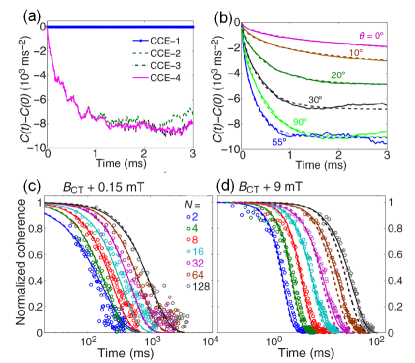
Figure 8: Experimental test of Gaussian noise model in ^natSi:Bi system. (a) Relative auto-correlation function $C(t)-C(0)$ of the ²⁹Si nuclear spin bath at the “clock” transtion of bisumth donors in silicon ($B_{\mathrm{CT}}=79.9$ mT) calculated by the CCE method (CCE-$M$ denotes the $M$th-order CCE truncation by keeping cluster correlations up to a certain size $M$, see Sec. VIII.4.4 for details). Here a specific nuclear spin configuration is chosen with the external magnetic field $\mathbf{B}\parallel[110]$. (b) $C(t)-C(0)$ (solid lines) at the “clock” transtion for several magnetic field orientations in the $[001]-[110]$ plane with $\theta=0^{\circ}$ corresponding to [001]. Results are obtained by averaging over 50 different nuclear spin configurations. Dashed lines are fits of the form $\Delta^{2}\{\text{exp}[-(|t|/\tau)^{n}]-1\}$. (c,d) Comparisons of electron spin decoherence obtained by the quantum model (solid lines), the semiclassical model (dashed lines), and the experimental measurement (circles) for the magnetic fields near the “clock” transtion. Here $N$=2, 4, 8, 16, 32, 64, 128 corresponds to the DD control CPMG-2, XY-4, XY-8, XY-16, (XY-16)$\times$2, (XY-16)$\times$4, (XY-16)$\times$8. In theoretical calculations, CPMG-$N$ is equivalent to XY-DD. Extracted from Refs. Ma et al. (2015).

The DD noise spectroscopy method based on the Gaussian noise model has been widely used to characterize the baths Álvarez and Suter (2011); Bylander et al. (2011); Bar-Gill et al. (2012). The main idea is to use a specific DD control sequence (such as CPMG-$N$ with large $N$) with the filter function approximated as a Dirac delta function at $\omega_{0}=\pm\pi{N}/t_{\mathrm{d}}$ [see Fig. 9(a)],

$$t_{\mathrm{d}}F(\omega t_{\mathrm{d}})\approx\pi[\delta(\omega-\omega_{0})+\delta(\omega+\omega_{0})],$$

Then following Eqs. (28) and  (29), the bath noise spectrum can be determined as

$$S(\pm\omega_{0})=-2\mathrm{ln}[L(t_{\mathrm{d}})]/t_{\mathrm{d}}.$$

However, this method can reproduce a meaningful bath noise spectrum only if the the bath can be descibed by a semiclassical Gaussian noise model. For example, in the ${}^{\text{nat}}$Si:Bi system, we use the DD noise spectroscopy method to determine the effective noise spectra corresponding to the CPMG-100 case, and then use the derived noise spectra to calculate the spin decoherence under other DD control sequences Ma et al. (2015). Close to the “clock” transition, the nuclear spin bath produces approximately a Gaussian noise, then the DD noise spectroscopy method can not only reproduce the spin decoherence curves for other DD control [see Fig. 9(b)], but also well reproduce the exact noise spectrum obtained from exact quantum calculations [Fig. 9(c)]. However, far away from the “clock” transition, the Gaussian noise appromiation is not valid any more, so we find increasing discrepancies between the exact decoherence model and the semiclassical model using the DD noise spectroscopy method as the pulse number of CPMG-$N$ deviates from 100 [Fig. 9(d)].

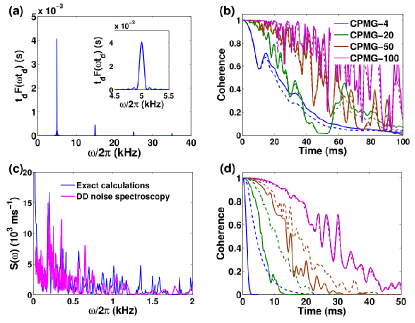
Figure 9: (a) Filter function $t_{\mathrm{d}}F(\omega t_{\mathrm{d}})$ for CPMG-100 noise spectroscopy with $t_{\mathrm{d}}=10$ ms. (b) Calculated Bi donor electron spin decoherence under an exact quantum model (solid lines) and semiclassical model obtained from noise spectroscopy of the CPMG-100 DD (dashed lines), evaluated close to the “clock” transition ($B_{\text{CT}}+10$ G). (c) Comparison of the noise spectrum from the CPMG-100 spectral decomposition in (b) to the exact one from CCE calculations. (d) similar to (b) but for the magentic field far from the “clock” transition ($B_{\text{CT}}+1000$ G). Extracted from Refs. Ma et al. (2015).

VI Quantum picture of central spin decoherence

Up to now, we have given two different interpretations of central spin decoherence. First, random modulation of the central spin’s transition frequency by classical noises (Sec. III) or quantum noises (Sec. V). Second, random state collapes of the central spin due to measurement by the environment (Sec. II), but the environment is not explicitly treated there. In this section, we give a full quantum picture Witzel and Das Sarma (2006); Yao et al. (2006); Yang and Liu (2008b) that substantiates the previous intuitive measurement interpretation of central spin decoherence.

The starting point is the general pure-dephasing Hamiltonian in Eq. (32) for the closed quantum system consisting of the central spin and the bath Yao et al. (2006); Liu et al. (2007); Yao et al. (2007):

$$\hat{H}=\hat{S}_{z}\hat{b}+\hat{H}_{B}=\hat{H}_{+}|\uparrow\rangle\langle\uparrow|+\hat{H}_{-}|\downarrow\rangle\langle\downarrow|,$$ (43)

where $\hat{H}_{\pm}\equiv\hat{H}_{B}\pm\hat{b}/2$ are the bath Hamiltonians depending on the central spin states being $|\uparrow\rangle$ or $|\downarrow\rangle$. The initial state of the bath is the maximally mixed thermal state [Eq. (33)]. However, central spin decoherence under DD control is usually insensitive to the initial state of the bath (as discussed in Sec. V.2). This allows us to take a pure state $|J\rangle$ sampled from the thermal ensemble (see Eq. (33)) as the initial state of the bath to provide a transparent quantum picture of decoherence Yao et al. (2006); Liu et al. (2007); Yao et al. (2007). Note that a pure initial state of the bath can in principle be prepared via special methods such as quantum measurements of the bath Giedke et al. (2006); Klauser et al. (2006); Stepanenko et al. (2006); Cappellaro (2012); Shulman et al. (2014) and nonlinear feedback Greilich et al. (2007); Xu et al. (2009); Sun et al. (2012); Latta et al. (2009); Bluhm et al. (2010); Togan et al. (2011); Yang and Sham (2012, 2013).

VI.1 Decoherence as a result of measurement by environment

Now the initial state of the whole system is the product of the central spin state $|\psi\rangle=C_{+}|\uparrow\rangle+C_{-}|\downarrow\rangle$ and the pure bath state $|J\rangle$. The bath undergoes bifurcated evolution $|J\rangle\rightarrow|J_{\pm}(t)\rangle\equiv e^{-i\hat{H}_{\pm}t}|J\rangle$ [Fig. 10(a)], and the coupled system evolves into an entangled state

$$|\Psi(t)\rangle\equiv C_{+}|\uparrow\rangle\otimes|J_{+}(t)\rangle+C_{-}|\downarrow\rangle\otimes|J_{-}(t)\rangle.$$ (44)

During this process, the population of the unperturbed central spin eigenstates $|\uparrow\rangle$ and $|\downarrow\rangle$ remains unchanged, but the off-diagonal coherence

$$L(t)=\langle J_{-}(t)|J_{+}(t)\rangle=\langle J|e^{i\hat{H}_{-}t}e^{-i\hat{H}_{+}t}|J\rangle$$ (45)

generally decays due to the bifurcated bath evolution Yao et al. (2006); Liu et al. (2007); Yao et al. (2007). From the viewpoint of quantum measurement Brune et al. (1996); Zurek (2003), the central spin state $|\uparrow\rangle$ ($|\downarrow\rangle$) is recorded in the bath pathway $|J_{+}(t)\rangle$ ($|J_{-}(t)\rangle$). The off-diagonal coherence between $|\uparrow\rangle$ and $|\downarrow\rangle$ is the overlap between these two pathways of the bath. Below we discuss two specific cases.

1. $[\hat{b},\hat{H}_{B}]=0$. The bath initial state $|J\rangle$ can be chosen as a common eigenstates of $\hat{H}_{B}$ and $\hat{b}$, with eigenvalues $\varepsilon_{J}$ and $b_{J}$, respectively. Then the two pathways $|J_{\pm}(t)\rangle=e^{-i(\varepsilon_{J}\pm b_{J}/2)t}|J\rangle$ are identical up to a phase factor and completely indistinguishable. There is no quantum entanglement between the central spin and the bath, and the central spin coherence $L(t)=e^{-ib_{J}t}$ does not decay, but just acquires a phase due to the static noise field $b_{J}$, consistent with the discussions in Sec. V.1.

2. $[\hat{b},\hat{H}_{B}]\neq 0$. The initial state $|J\rangle$, if taken as an eigenstate of $\hat{H}_{B}$, in general is not an eigenstate of $\hat{b}$, so it undergoes bifurcated evolution into different pathways $|J_{\pm}(t)\rangle$. Correspondingly, the central spin coherence $L(t)\approx\langle J_{-}(t)|J_{+}(t)\rangle$ decays due to the bifurcated bath evolution and hence quantum entanglement between the central spin and the bath. Using $e^{-i\hat{H}_{+}t}=e^{-i\hat{H}_{B}t}\mathcal{T}e^{-(i/2)\int_{0}^{t}\hat{b}(t^{\prime})dt^{\prime}}$ and $e^{i\hat{H}_{-}t}=\mathcal{\bar{T}}e^{-(i/2)\int_{0}^{t}\hat{b}(t^{\prime})dt^{\prime}}e^{i\hat{H}_{B}t}$, we immediately see that $\langle J_{-}(t)|J_{+}(t)\rangle$ is just the “true” decoherence $L_{\mathrm{dyn}}(t)$ caused by the dynamical quantum noise [Eq. (36)], which has been discussed in Sec. V.2. When the two pathways of the bath become orthogonal and hence completely distinguishable at a certain time, the central spin is perfectly measured by the bath and its off-diagonal coherence vanishes completely.

Finally, we note that upon decomposing the bath states into the unnormalized common part and the unnormalized difference part as $|J_{\pm}(t)\rangle\equiv|\tilde{J}_{\mathrm{nc}}(t)\rangle\pm|\tilde{J}_{\mathrm{c}}(t)\rangle$, the entangled state can be rewritten as

$$|\Psi(t)\rangle=|\psi\rangle\otimes|\tilde{J}_{\mathrm{nc}}(t)\rangle+\hat{\sigma}_{z}|\psi\rangle\otimes|\tilde{J}_{\mathrm{c}}(t)\rangle,$$ (46)

i.e., the central spin state $|\psi\rangle$ and the phase-flipped state $\sigma_{z}|\psi\rangle$ are recorded in the unnormalized bath states $|\tilde{J}_{\mathrm{nc}}(t)\rangle$ and $|\tilde{J}_{\mathrm{c}}(t)\rangle$, respectively. If $|\tilde{J}_{\mathrm{c}}(t)\rangle$ is orthogonal to $|\tilde{J}_{\mathrm{nc}}(t)\rangle$, then the central spin density matrix would be an incoherent mixture of $\sqrt{\langle\tilde{J}_{\mathrm{nc}}(t)|\tilde{J}_{\mathrm{nc}}(t)\rangle}|\psi\rangle\equiv\hat{M}_{\mathrm{nc}}|\psi\rangle$ and $\sqrt{\langle\tilde{J}_{\mathrm{c}}(t)|\tilde{J}_{\mathrm{c}}(t)\rangle}\hat{\sigma}_{z}|\psi\rangle\equiv\hat{M}_{\mathrm{c}}|\psi\rangle$, which recovers our intuitive discussion for Markovian environmental noise in Sec. II.4.

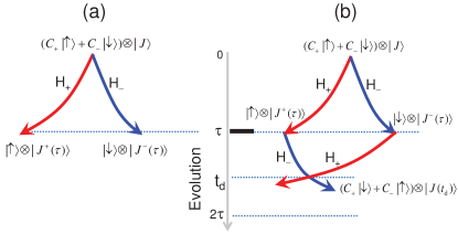
Figure 10: Schematic illustration of the bifurcated bath evolution pathways dependent on the central spin states: (a) for FID; (b) for the central spin being flipped by a $\pi$-pulse at an intermediate time. Here the initial state of the spin bath is assumed to be a pure state $|J\rangle$.

VI.2 Coherence recovery by dynamical decoupling

To recover the central spin coherence lost into the bath, it is necessary to erase the measurement information by making the two bath pathways $|J_{\pm}(t)\rangle$ identical up to a phase factor. For this purpose, the simplest approach is Hahn echo Hahn (1950), in which a $\pi$-pulse is applied to the central spin at time $\tau$ to exchange the evolution direction of the two pathways [see Fig. 10(b)]. At $t>\tau$, the two pathways are $|J_{\pm}(t)\rangle=e^{-i\hat{H}_{\mp}(t-\tau)}e^{-i\hat{H}_{\pm}\tau}|J\rangle$ and the coupled system evolves into $|\Psi(t)\rangle=C_{+}|\downarrow\rangle\otimes|J_{+}(t)\rangle+C_{-}|\uparrow\rangle\otimes|J_{-}(t)\rangle$. The intersection of the two pathways $|J_{+}(t_{\mathrm{d}})\rangle\approx e^{i\varphi}|J_{-}(t_{\mathrm{d}})\rangle$ at a certain time $t_{\mathrm{d}}$ would erase the measurement information and restores the central spin coherence, as shown in Fig. 10(b) Yao et al. (2006); Liu et al. (2007); Yao et al. (2007).

Under a general DD characterized by the DD modulation function $s(t)$, by working in the interaction picture defined by the control Hamiltonian (Eq. (25)), the total Hamiltonian becomes $\hat{H}_{B}+s(t)\hat{b}\hat{S}_{z}$. The two bath pathways start from $|J\rangle$ and bifurcate into $|J_{\pm}(t_{\mathrm{d}})\rangle=\hat{U}_{\pm}(t_{\mathrm{d}})|J\rangle$, where $\hat{U}_{\pm}(t_{\mathrm{d}})\equiv\mathcal{T}e^{-i\int_{0}^{t_{\mathrm{d}}}[\hat{H}_{B}\pm s(t)\hat{b}/2]dt}$ are the bifurcated bath evolution operators. Then the central spin coherence is

$$L(t_{\mathrm{d}})=\langle J|\hat{U}_{-}^{\dagger}(t_{\mathrm{d}})\hat{U}_{+}(t_{\mathrm{d}})|J\rangle.$$ (47)

For example, the FID $L(t)=\langle J|e^{i\hat{H}_{-}\tau}e^{-i\hat{H}_{+}\tau}|J\rangle$ and Hahn echo $L(t_{\mathrm{d}}=2\tau)=\langle J|e^{i\hat{H}_{-}\tau}e^{i\hat{H}_{+}\tau}e^{-i\hat{H}_{-}\tau}e^{-i\hat{H}_{+}\tau}|J\rangle$. For $[\hat{b},\hat{H}_{B}]=0$, as long as $t_{\mathrm{d}}$ satisfy the echo condition (Eq. (27)), we have $|J_{\pm}(t_{\mathrm{d}})\rangle=e^{-i\varepsilon_{J}t_{\mathrm{d}}}|J\rangle$ and hence $L(t_{\mathrm{d}})=1$, i.e., the phase due to the static noise field $b_{J}$ is completely refocused.

VI.3 Ensemble average

In practice, we should use the thermal state $\hat{\rho}_{B}^{\mathrm{eq}}$ [Eq. (33)] as the initial state of the bath, then we recover the results in Sec. V.2. The FID as given by Eq. (35) is the product of inhomogenous dephasing due to the thermal noise [Eq. (7)] and “true” decoherence due to the quantum noise (Eq. (36) or Eq. (45)) that is almost independent of $|J\rangle$ Yao et al. (2006); Zhao et al. (2012b); Ma et al. (2015). Under DD, the former is removed, so $L(t_{\mathrm{d}})=\langle J_{-}(t_{\mathrm{d}})|J_{+}(t_{\mathrm{d}})\rangle$ is “true” decoherence due to the quantum noise [Eq. (39) or (47)].

The discussions above for a central spin-1/2 can be easily generalized to a general multi-level system with eigenstates $\{|n\rangle\}$ and the pure-dephasing Hamiltonian $\sum_{m}\hat{H}_{m}|m\rangle\langle m|$ Zhao et al. (2011b); Ma et al. (2015). The off-diagonal coherence $L_{n,m}(t)\equiv\langle n|\hat{\rho}(t)|m\rangle$ for a given quantum transition $|m\rangle\leftrightarrow|n\rangle$ can be mapped to that of a central spin-1/2 once the states $\{|m\rangle,|n\rangle\}$ are identified as $\{|\uparrow\rangle,|\downarrow\rangle\}$ with $\hat{H}_{B}\equiv(\hat{H}_{m}+\hat{H}_{n})/2$ and $\hat{b}\equiv\hat{H}_{m}-\hat{H}_{n}$.

VII Physical systems

Electron spins localized in solid-state nanostructures are promising candidates of qubits for quantum information processing and quantum sensing. These “artificial atoms” occur when the impurities or defects in semiconductor nanostructures produce localized potentials to confine one or a few electrons or holes (i.e., an empty electron state in the valence band of semiconductors), analagous to electrons bound to atomic nuclei. For such electron spins, the most relevant environments are the phonon bath and the nuclear spins of the host lattices. The electron spins couple indirectly to the phonon baths via spin-orbit coupling, and couples directly to the nuclear spin baths via the hyperfine interaction (HFI). In this section, we first introduce these interactions and then review central spin decoherence due to these interactions in typical semiconductor nanostructures.

VII.1 Phonon and spin baths

VII.1.1 Phonon scattering via spin-orbit coupling

Electric fields are not directly coupled to the electron spin $\hat{\mathbf{S}}$. Indirect coupling occurs due to the relativistic correction

$$\hat{H}_{\mathrm{so}}=\frac{1}{2m_{0}^{2}c^{2}}(\nabla V(\hat{\mathbf{r}})\times\hat{\mathbf{p}})\cdot\hat{\mathbf{S}}$$

to the non-relativistic Hamiltonian for the electron moving in a potential $V(\mathbf{r})$. Due to this spin-orbit coupling term, the electron spin eigenstates become mixtures of spin and orbital states, thus fluctuating electric fields can induce transitions between these eigenstates (i.e., spin relaxation) Khaetskii and Nazarov (2000, 2001); Woods et al. (2002) and randomly modulate the transition frequency (i.e., pure dephasing) Golovach et al. (2004); Semenov and Kim (2004). In carefully designed systems (where the charge fluctuations are suppressed), the most relevant source of electrical noises is the lattice vibration (i.e., the phonon bath). The phonon energy spectrum ranges over a few tens of meV, much larger than the electron spin transition energy ($\sim\mathrm{\mu eV})$, so the phonon noise is Markovian and usually limits the electron spin $T_{1}$ and, at high temperatures, also limits the electron spin $T_{2}$ (see Sec. II). At low temperatures and in light-element materials where spin-orbit coupling is weak, phonon scattering is suppressed and the experimentally measured electron spin $T_{1}$ is very long, ranging from tens of microseconds up to seconds (see Hanson et al. (2007) for a review). At low temperautre, the phonon-limited electron spin $T_{2}$ is estimated as $T_{2}\approx 2T_{1}$ Golovach et al. (2004), but the experimentally measured $T_{2}$ is much shorter as limited by the hyperfine interaction with the nuclear spin bath.

VII.1.2 Hyperfine interaction

	75As	$\ {}^{113}$In	115In	69Ga	71Ga
Spin moment $I_{\alpha}$	$3/2$	$9/2$	$9/2$	$3/2$	$3/2$
Abundance $f_{\alpha}$	$100\%$	$4.28\%$	$95.72\%$	$60.1\%$	$39.9\%$
$\gamma_{\alpha}$ (10-3 rad ns-1T-1)	$45.8$	$58.5$	$58.6$	$64.3$	$81.8$
$A_{\alpha}$ (rad ns${}^{-1})$	$69.8$	$85.1$	$85.3$	$56$	$73$
$Q_{\alpha}$ (10-31 m2)	$314$	$759$	$770$	$171$	$107$

Table 1: Spin moment, natural abundance, gyromagnetic ratio, HFI constant, and quadrupole moment of some isotopes that appear in III-V semiconductor quantum dots (QDs), with the reduced Planck constant $\hbar=1$ and hence $1\ \mathrm{\mu eV}\approx 1.52$ ns^-1. The quadrupole moments are from Ref. Pyykko (2008). Other data for In and As are from Ref. Liu et al. (2007), while those for Ga are from Refs. Paget et al. (1977) and Coish and Baugh (2009).

For a nuclear spin $\hat{\mathbf{I}}_{n\alpha}$ of species $\alpha$ located at $\mathbf{R}_{n\alpha}$, its magnetic moment $\gamma_{\alpha}\hat{\mathbf{I}}_{n\alpha}$ produces a vector potential $\mathbf{A}_{n\alpha}=(\mu_{0}/4\pi)(\gamma_{\alpha}\hat{\mathbf{I}}_{n\alpha}\times\boldsymbol{\rho}_{n\alpha})/\rho_{n\alpha}^{3}$ at the location $\mathbf{r}$ of the electron with $\boldsymbol{\rho}_{n\alpha}\equiv\mathbf{r}-\mathbf{R}_{n\alpha}$. The total vector potential $\mathbf{A}\equiv\sum_{n\alpha}\mathbf{A}_{n\alpha}$ due to all the nuclei gives rise to the electron-nuclear magnetic coupling $\gamma_{e}(\hat{\mathbf{p}}\cdot\mathbf{A}+\mathbf{A}\cdot\hat{\mathbf{p}})/2+\gamma_{e}\hat{\mathbf{S}}\cdot(\nabla\times\mathbf{A})$ Abragam (1961), which is the sum of the contact HFI

$$\hat{H}_{\mathrm{c}}=\frac{2\mu_{0}}{3}\sum_{n\alpha}\gamma_{e}\gamma_{\alpha}\hat{\mathbf{I}}_{n\alpha}\cdot\hat{\mathbf{S}}\delta(\boldsymbol{\rho}_{n\alpha}),$$

the dipolar HFI

$$\hat{H}_{\mathrm{d}}=\frac{\mu_{0}}{4\pi}\sum_{n\alpha}\gamma_{e}\gamma_{\alpha}\left(3\frac{(\hat{\mathbf{S}}\cdot\boldsymbol{\rho}_{n\alpha})(\hat{\mathbf{I}}_{n\alpha}\cdot\boldsymbol{\rho}_{n\alpha})}{\rho_{n\alpha}^{5}}-\frac{\hat{\mathbf{S}}\cdot\hat{\mathbf{I}}_{n\alpha}}{\rho_{n\alpha}^{3}}\right),$$

and the nuclear-orbital interaction

$$\hat{H}_{\mathrm{orb}}=\frac{\mu_{0}}{4\pi}\sum_{n\alpha}\gamma_{e}\gamma_{\alpha}\frac{\hat{\mathbf{L}}_{n\alpha}\cdot\hat{\mathbf{I}}_{n\alpha}}{\rho_{n\alpha}^{3}},$$

where $\gamma_{e}\approx 1.76\times 10^{11}$ rad/(s T) is the electron gyromagnetic ratio (positive) for free electrons and $\hat{\mathbf{L}}_{n\alpha}\equiv\boldsymbol{\rho}_{n\alpha}\times\hat{\mathbf{p}}$ is the electron orbital angular momentum around the nucleus. The magnetic interaction involves the coupling of the electron orbital and electron spin to the nuclear spin. At low temperature, the localized electron in a nanostructure stays in its ground orbital $\psi(\mathbf{r})$, so the magnetic interaction should be averaged over $\psi(\mathbf{r})$ to yield the effective spin-spin interaction.

The spin-spin contact HFI

$$\bar{H}_{\mathrm{c}}=\langle\psi|\hat{H}_{\mathrm{c}}|\psi\rangle=\sum_{n\alpha}a_{n\alpha}\hat{\mathbf{S}}\cdot\hat{\mathbf{I}}_{n\alpha},$$ (48)

where the HFI coefficient $a_{n\alpha}=(2\mu_{0}/3)\gamma_{e}\gamma_{\alpha}|\psi(\mathbf{R}_{n\alpha})|^{2}$ is determined by the electron density at the site of the nucleus. The contact HFI is strong for electrons in the conduction band of III-V semiconductors (mostly $s$-orbital) and silicon (hybridization of $s$, $p$, and $d$ orbitals), but vanishes in graphene, carbon nanotubes, and the valence band of III-V semiconductors since their primary component – the $p$-orbital – vanishes at the site of the nucleus Coish and Baugh (2009). For III-V semiconductors with a non-degenerate $s$-orbital conduction band minumum at the $\Gamma$ point, the ground orbital can be written as $\psi(\mathbf{r})$ $=\sqrt{\Omega}F(\mathbf{r})u_{c}(\mathbf{r})$, where $\Omega$ is the unit cell volume, $F(\mathbf{r})$ is the slowly-varying envelope function normalized as $\int|F(\mathbf{r})|^{2}d\mathbf{r}=1$, and $u_{c}(\mathbf{r})$ is the $s$-orbital band-edge Bloch function that is conveniently normalized as $\int_{\Omega}|u_{c}(\mathbf{r})|^{2}d\mathbf{r}=1$, such that $d_{\alpha}\equiv|u_{c}(\mathbf{R}_{n\alpha})|^{2}$ is the electron density on the nucleus of species $\alpha$ Paget et al. (1977). So the HFI coefficient becomes $a_{n\alpha}=A_{\alpha}\Omega|F(\mathbf{R}_{n\alpha})|^{2}$, where

$$A_{\alpha}=\frac{2\mu_{0}}{3}\gamma_{e}\gamma_{\alpha}d_{\alpha}$$ (49)

is the HFI constant that only depends on the species of the nuclear spin (through $\gamma_{\alpha}$) and the semiconductor material (through $d_{\alpha}$). The numerical values of $\gamma_{\alpha}$ and $A_{\alpha}$ for some relevant isotopes in III-V semiconductor quantum dots (QDs) are listed in Table 1. For silicon, there are six equivalent conduction band minima at $\mathbf{k}_{\lambda}=\pm k_{0}\mathbf{e}_{x}$, $\pm k_{0}\mathbf{e}_{y}$, $\pm k_{0}\mathbf{e}_{z}$, where $k_{0}\equiv 0.85(2\pi/a_{\operatorname{Si}})$ and $a_{\operatorname{Si}}=5.43$ $\operatorname{\text{\AA}}$ is the lattice constant of silicon. Thus the ground orbital of a hydrogen-like donor in silicon is $\psi(\mathbf{r})=(1/\sqrt{6})\sum_{\lambda}F_{\lambda}(\mathbf{r})u_{\lambda}(\mathbf{r})e^{i\mathbf{k}_{\lambda}\cdot\mathbf{r}}$, where $u_{\lambda}(\mathbf{r})e^{i\mathbf{k}_{\lambda}\cdot\mathbf{r}}$ is the Bloch function at the $\lambda$th minimum consisting of $s$, $p$, and $d$ orbitals, with the normalization $\int_{\Omega}|u_{\lambda}(\mathbf{r})|^{2}d\mathbf{r}=\Omega$. The hydrogen-like envelope function associated with $\pm k_{0}\mathbf{e}_{x}$ is Feher (1959); de Sousa and Das Sarma (2003b)

$$F_{x}(\mathbf{r})=\frac{1}{\sqrt{\pi(na)^{2}nb}}e^{-\sqrt{x^{2}/(nb)^{2}+(y^{2}+z^{2})/(na)^{2}}},$$

with similar expressions for $F_{y}(\mathbf{r})$ and $F_{z}(\mathbf{r})$ by appropriate permutations of $x,y,z$. Here $a=25.09$ $\operatorname{\text{\AA}}$ and $b=14.43$ $\operatorname{\text{\AA}}$ are characteristic lengths for hydrogenic impurities in silicon, $n=0.81$ ($0.64$) for phosphorus (bismuth) donors de Sousa and Das Sarma (2003b); Richard et al. (2004); Zwanenburg et al. (2013). The donor electron density at the silicon lattice site $\mathbf{R}_{n}$ is given by Feher (1959) $|\psi(\mathbf{R}_{n})|^{2}=(2d_{\operatorname{Si}}/3)[\sum_{\alpha=x,y,z}F_{\alpha}(\mathbf{R}_{n})\cos(k_{0}\mathbf{R}_{n}\cdot\mathbf{e}_{\alpha})]^{2}$, where $d_{\operatorname{Si}}\equiv|u_{\lambda}(\mathbf{R}_{n})|^{2}\approx 186$ is the electron density on the silicon site in silicon crystal Shulman and Wyluda (1956); de Sousa and Das Sarma (2003b).

The spin-spin dipolar HFI

$$\bar{H}_{\mathrm{d}}=\langle\psi|\hat{H}_{\mathrm{d}}|\psi\rangle=\sum_{n\alpha}\hat{\mathbf{S}}\cdot\mathbf{A}_{n\alpha}\cdot\hat{\mathbf{I}}_{n\alpha},$$ (50)

where the dipolar HFI tensor

$$[\mathbf{A}_{n\alpha}]_{i,j}\equiv\frac{\mu_{0}}{4\pi}\gamma_{e}\gamma_{\alpha}\int\frac{|\psi(\mathbf{r})|^{2}}{\rho_{n\alpha}^{3}}\left(\frac{3\rho_{n\alpha}^{i}\rho_{n\alpha}^{j}}{\rho_{n\alpha}^{2}}-\delta_{ij}\right)d\mathbf{r}$$

with $i,j=x,y,z$. The dipolar HFI and the nuclear-orbital interaction $\bar{H}_{\mathrm{orb}}\equiv\langle\psi|\hat{H}_{\mathrm{orb}}|\psi\rangle$ are negligible for the $s$-orbital conduction band of III-V semiconductors. They become appreciable for donors in silicon (due to significant $p$- and $d$-orbital components in the band-edge Bloch functions) and even dominates for electrons in graphene, carbon nanotubes, and the valence band of III-V semiconductors Coish and Baugh (2009); Fischer et al. (2008); Testelin et al. (2009); Chekhovich et al. (2011, 2013), where the atomic $p$-orbital is the primary component of the Bloch functions and hence the contact HFI vanishes. If $\psi(\mathbf{r})$ is localized in the vicinity of $\mathbf{\bar{r}}$ and far from the nucleus, then the dipolar HFI $\bar{H}_{\mathrm{d}}=\langle\psi|\hat{H}_{\mathrm{d}}|\psi\rangle=\hat{H}_{\mathrm{d}}|_{\mathbf{r}\rightarrow\mathbf{\bar{r}}}$ reduces to the magnetic dipolar interaction between two point-like magnetic moments; while if $\psi(\mathbf{r})$ overlaps the nucleus, then $\bar{H}_{\mathrm{d}}$ is dominated by the interaction of the nuclear spin with the on-site electron spin density Testelin et al. (2009). Recently the manipulation and decoherence of valence band electrons (i.e., holes) in QDs is under active study (see Ref. Chesi et al. (2014) for a review).

VII.1.3 Intrinsic nuclear spin interactions

The interaction between nuclear spins have been well studied in NMR experiments and in theories (for a review, see Ref. Slichter (1990)). The direct magnetic dipolar interaction has the dipolar form

$$\hat{H}_{\mathrm{NN}}^{d}=\frac{1}{2}\sum_{n\alpha\neq m\beta}\frac{\mu_{0}}{4\pi}\gamma_{\alpha}\gamma_{\beta}\left(\frac{\hat{\mathbf{I}}_{n\alpha}\cdot\hat{\mathbf{I}}_{m\beta}}{R^{3}}-\frac{3(\hat{\mathbf{I}}_{n\alpha}\cdot\mathbf{R})(\hat{\mathbf{I}}_{m\beta}\cdot\mathbf{R})}{R^{5}}\right),$$ (51)

where $\mathbf{R}\equiv\mathbf{R}_{n\alpha}-\mathbf{R}_{m\beta}$ is the relative displacement between the locations $\mathbf{R}_{n\alpha}$ and $\mathbf{R}_{m\beta}$ of the two nuclei. The indirect nuclear interaction is mediated by virtual excitation of electron-hole pairs due to the HFI between nuclei and valence electrons Bloembergen and Rowland (1955); Shulman et al. (1955, 1957, 1958); Sundfors (1969). When the virtual excitation is caused by the contact HFI, the indirect coupling has the isotropic exchange form $\hat{H}_{\mathrm{NN}}^{\mathrm{ex}}=-B_{n\alpha,m\beta}^{\mathrm{ex}}\hat{\mathbf{I}}_{n\alpha}\cdot\hat{\mathbf{I}}_{m\beta}$, where $B_{n\alpha,m\beta}^{\mathrm{ex}}$ is determined by the band structure of the material. When the virtual excitation of electron-hole pairs involves both the contact and dipolar HFI, the indirect nuclear spin coupling has the same form as the direct dipolar interaction in Eq. (51) except for a multiplicative factor that depends on the inter-nuclear distance. When the virtual excitation is caused by the dipolar HFI alone, the indirect coupling is the sum of an isotropic exchange term and dipole-dipole term. Except for the direct dipolar coupling, experimental characterization of indirect couplings is very limited.

	$\ \mathrm{\mu s}^{-1}$	$\ \mathrm{\mu eV}$	mK
Electron Zeeman splitting	$10^{5}$	$10^{2}$	$10^{3}$
Nuclear Zeeman splitting	$50$	$0.05$	$0.5$
Hyperfine interaction	$1$	$10^{-3}$	$10^{-2}$
N-N dipolar interaction	$10^{-4}$	$10^{-7}$	$10^{-6}$

Table 2: Characteristic energy scales in an InAs QD with dimensions $35\times 35\times 6$ nm³ under a magnetic field of 1 T Liu et al. (2007), with $\hbar$=1.

Due to the vanishing electric dipole moment of the nucleus, the nuclear spin is not coupled to constant electric fields. However, a nucleus with spin $I>1/2$ has a finite electric quadrupole moment, so a nuclear spin $\hat{\mathbf{I}}$ located at $\mathbf{R}$ with quadrupole moment $Q$ is coupled to the on-site electric field gradient tensor $V_{ij}\equiv\partial^{2}V(\mathbf{x})/\partial x_{i}\partial x_{j}|_{\mathbf{x}=\mathbf{R}}$ through $\hat{H}_{Q}=\sum_{ij=x,y,z}V_{ij}\hat{Q}_{ij}$, where Abragam (1961)

$$\hat{Q}_{ij}\equiv\frac{eQ}{6I(2I-1)}\left[\frac{3}{2}(\hat{I}_{i}\hat{I}_{j}+\hat{I}_{j}\hat{I}_{i})-\delta_{ij}I(I+1)\right]$$

is the nuclear spin quadrupole tensor. In the principal axis $OXYZ$ of the electric field gradient tensor, only diagonal components $V_{XX},V_{YY},V_{ZZ}$ survives. Using the non-axial parameter $\eta\equiv(V_{XX}-V_{YY})/V_{XX}$ and Laplace equation $V_{XX}+V_{YY}+V_{ZZ}=0$ allows the quadrupolar interaction to be simplified to Abragam (1961)

$$\hat{H}_{Q}=\frac{eQV_{ZZ}}{4I(2I-1)}\left[3\hat{I}_{Z}^{2}-I(I+1)+\eta(\hat{I}_{X}^{2}-\hat{I}_{Y}^{2})\right].$$

The quadrupole moments of some relevant isotopes in III-V QDs are listed in Table I.

In a crystal with cubic symmetry, the electric field gradient tensor obey $V_{XX}=V_{YY}=V_{ZZ}$, which together with the Laplace equation dictates vanishing electric field gradient and quadrupolar interaction. Nonzero quadrupolar interaction could arise from broken cubic symmetry by lattice distortion due to semiconductor heterostructure, dopants, or defects. The quadrupolar interactions have important effects on the nuclear spin dynamics Abragam (1961) and hence the auto-correlations of the noises on a central electron spin coupled to the nuclear spin bath Sinitsyn et al. (2012). Recently Chekhovich et al. measured Chekhovich et al. (2012) strain-induced quadrupolar interactions in self-assembled QDs and found that they suppress the nuclear spin flip-flops Chekhovich et al. (2015), while in gate-defined GaAs QDs, the quadrupolar interaction was found to reduce the electron spin coherence time by causing faster decorrelation of the nuclear spin noise Botzem et al. (2016).

VII.2 Electron spin decoherence in solid-state nano-systems

The widely studied systems include semiconductor QDs Kastner (1993); Loss and DiVincenzo (1998); Gupta et al. (1999), phosphorus and bismuth donors in silicon Kane (1998); Tyryshkin et al. (2006); George et al. (2010), and nitrogen-vacancy (NV) centers in diamond Gruber et al. (1997); Doherty et al. (2013). In these systems, electron or hole spins act as qubits. At low temperatures, the spin-phonon scattering processes are largely suppressed Khaetskii and Nazarov (2000, 2001); Golovach et al. (2004); Bulaev and Loss (2005), so the main noise source for electron spin qubits in these systems are the nuclear spin baths of the host lattice. As a convention, we use $T_{2}^{\ast}$ for the dephasing time in FID (since FID is usually dominated by inhomogeneous dephasing), and use $T_{2}$ for the dephasing time under various DD controls, where inhomogeneous dephasing has been removed.

VII.2.1 Semiconductor quantum dots

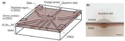
Figure 11: (a) A gate-defined double quantum dots, with 2DEG for two-dimensional electron gas. (b) A self-assembled quantum dot. Scale bar $\sim$5 nm. Extracted from Fig. 1 of Ref. Hanson and Awschalom (2008).

Electron spins in QDs are among the earliest candidates for quantum computing Loss and DiVincenzo (1998); Imamoğlu et al. (1999). A QD is a semiconductor nanostructure with size from a few to hundreds of nanometers. The electrons in QDs experience quantum confinement in all three spatial dimensions, with their energies, wave functions, and hence spin properties tunable by the QD size and shape Kouwenhoven et al. (2001); Reimann and Manninen (2002); Hanson et al. (2007). There are different ways to fabricate QDs, e.g., gate-defined QDs Kouwenhoven et al. (2001) confine electrons by an electrostatic potential from electric voltages on lithographically defined metallic gates [Fig. 11(a)], while self-assembled QDs Warburton (2013) confine electrons with a deep potential that is created during the random semiconductor growth process [Fig. 11(b)]. There are also QDs formed by interface fluctuation in GaAs/AlGaAs quantum well structures Gammon et al. (1991). The weakly confined electrons in gate-defined QDs can be controlled electrically at very low temperatures ($<1$ K), and strongly confined electrons in self-assembled QDs and interface fluctuation QDs can be controlled optically at a little higher temperatures ($\sim 4$ K).

A critical issue in electron spin qubits in III–V semiconductor QDs is the inevitable presence of nuclear spins in the semiconductor substrate since all stable isotopes of the III-V semiconductors have nonzero nuclear spins Khaetskii et al. (2002); Merkulov et al. (2002). The thermal noise (see Sec. V.1 and Sec. VI.3) from the nuclear spin bath leads to rapid inhomogeneous dephasing of the electron spin on a time scale $T_{2}^{\ast}\sim 10$ ns Hanson et al. (2007). When this inhomogeneous dephasing is removed by Hahn echo, the quantum dynamical noise from the nuclear spin bath still limits the electron spin dephasing time $T_{2}$ to a few microseconds Hanson et al. (2007). Fortunately, the nuclear spin noise has a rather long auto-correlation time $\tau_{c}\sim$ 1 ms ($\sim$ the inverse of nuclear spin interactions, see Table 2) , so it can be significantly suppressed by various DD sequences, e.g., the multi-pulse CPMG has extended the $T_{2}$ of a singlet-triplet qubit in gate-defined GaAs double QDs from $\sim 1$ $\mathrm{\mu s}$ Petta et al. (2005); Greilich et al. (2006); Koppens et al. (2008) to $\sim$ 1 ms Bluhm et al. (2011); Malinowski et al. (2016). Recently, silicon-based QDs have been developed, such as QDs in Si/SiGe heterostructures and gated nanowires (see Morton et al. (2011) for a review). As the only silicon isotope ²⁹Si that has non-zero spin is of low natural abundance ($4.7\%$), the measured electron spin $T_{2}^{\ast}\approx 360$ $\mathrm{ns}$ in Si/SiGe double QDs Maune et al. (2012) is longer than in GaAs QDs by more than one order of magnitude, and further improvements are expected for devices using isotopically enriched ²⁸Si.

VII.2.2 Donors in silicon and related materials

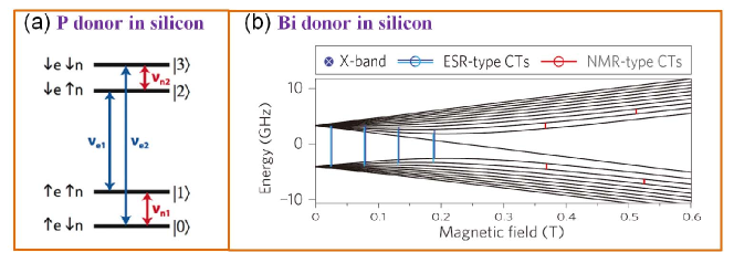
Figure 12: Energy levels of phosphorus and bismuth donors in silicon. (a) P donor electron spin-1/2 couples to the ³¹P nuclear spin-1/2 via a moderate HFI of strength $A=117.5$ MHz. (b) Bi donor electron spin-1/2 couples to the ²⁰⁹Bi nuclear spin-9/2 via strong HFI with a strength$A=1.745$ GHz. Panels (a) and (b) are adapted from Refs. Tyryshkin et al. (2006) and Wolfowicz et al. (2013), respectively.

As the dominant material in semiconductor industry, silicon provides a platform to accommodate both quantum and classical information technologies. Electron and nuclear spins of individual donors in silicon have been proposed as qubits ever since the early years of solid-state quantum information Kane (1998). After Kane’s infuential proposal, different architectures have been proposed in which electron spin Vrijen et al. (2000) and orbital Barrett and Milburn (2003); Hollenberg et al. (2004), nuclear spin Morton et al. (2011), an electron and its donor nuclear spin Skinner et al. (2003) are used as qubits.

Silicon has three stable isotopes: ²⁸Si (natural abundance $92.2\%$), ²⁹Si (natural abundance $4.7\%$), and ³⁰Si (natural abundance $3.1\%$), among which only ²⁹Si has a nonzero nuclear spin $I=1/2$, in sharp contrast to III-V group semiconductors where all isotopes have nonzero nuclear spins. The low concentration of spinful nuclear isotopes and weak spin–orbit coupling in silicon results in long electron spin coherence times compared to that of spin qubits in III-V group semiconductor QDs. For high-mobility two-dimensional electron systems, their $T_{1}$ and $T_{2}$ reach a few microseconds at low temperature Tyryshkin et al. (2005), limited by phonon scattering via spin-orbit coupling. When the electron spin is tightly bound to a donor, the spin-orbit coupling is further suppressed, so at low temperatures its $T_{1}$ can reach minutes to hours Feher and Gere (1959), while its $T_{2}$ is usually limited by $T_{1}$ process at high temperature, or by other donor electron spins and the sparse ²⁹Si nuclear spin bath at low temperature Klauder and Anderson (1962).

Among all the group-V dopants in silicon, phosphorus donors in natural silicon (${}^{\text{nat}}$Si:P) or isotopically purified ²⁸Si (²⁸Si:P) have been widely studied. Phosphorus has only one stable isotope ³¹P with nuclear spin $I=1/2$ [Fig. 12(a)]. The P donor electron spins was exhaustively studied almost sixty years ago in the first electron-nuclear double resonance experiment Feher (1959). At low donor concentrations, the electron $T_{1}$ increases dramatically with decreasing temperature, reaching thousands of seconds at low temperature $\sim 1$ K Feher and Gere (1959); Castner (1962); Tyryshkin et al. (2003); Morello et al. (2010), while the ³¹P nuclear spin relaxation time exceeds 10 hours Feher (1959). At low temperature, the extrapolated $T_{2}$ of an isolated ²⁸P donor electron spin from spin echo measurements can reach $60$ ms Tyryshkin et al. (2003), comparable with $T_{1}$ $\sim 280$ ms. In ${}^{\text{nat}}$Si:P system, $T_{2}$ of the P donor electron spin under spin echo control is limited by the ²⁹Si nuclear spin bath to $\sim 1$ ms Tyryshkin et al. (2003). Recently unprecedented long electron spin $T_{2}\approx 12$ s Tyryshkin et al. (2012) and nuclear spin dephasing time up to a few minutes were reported in ultrapure ²⁸Si crystals Morton et al. (2008); Steger et al. (2012); Muhonen et al. (2014). Due to its exceptional long relaxation and dephasing times, the ³¹P nuclear spin is a good candidate as long-lived quantum memory or combined with the donor electron spin into a hybrid quantum register [Fig. 12(a)] Skinner et al. (2003).

Recently bismuth donors in silicon (Si:Bi) has attracted much attention as it has a number of advantages over the P donors in silicon. Bismuth has one long-lived isotope ²⁰⁹Bi with nuclear spin $I=9/2$ [Fig. 12(b)]. Compared with the Si:P system, the Bi donors in silicon have a much larger nuclear spin $I=9/2$ and a much stronger on-site HFI $A=1.4754$ GHz Feher (1959) between the Bi electron spin and the ²⁰⁹Bi nuclear spin. The much stronger on-site HFI in Si:Bi strongly mixes the electron and the nuclear spin even under moderate magnetic field. This enables electron-nuclear hybrid qubit, where each level consists of nearly equal superpositions of the electronic and Bi nuclear spin components Morley et al. (2013). Consequently, the strong magnetic dipolar interaction between the electron spin and the microwave magnetic field can induce rapid NMR transitions on the nanosecond time scale, two orders of magnitude faster than conventional NMR Morley et al. (2010); George et al. (2010) and several orders of magnitude faster than the decoherence of the hybrid qubit $T_{2}\sim 0.5$ ms, limited by ²⁹Si nuclear spins. By tuning the magnetic field to the “clock” transition between hybridized levels, whose frequency is insensitive to variations in the magnetic field to first order, the electron spin coherence time $T_{2}$ of up to 3 s has been observed Wolfowicz et al. (2013).

VII.2.3 Nitrogen-vacancy centers in diamond and related systems

The negatively charged nitrogen-vacancy (NV) center in diamond consists of a substitutional nitrogen atom adjacent to a carbon vacancy, which has C_3v symmetry with the symmetry axis pointing from the nitrogen to the vacancy (NV axis) [Fig. 13(a)]. The ground state of the NV center ³A₂ is a spin triplet ($S=1$) with the degenerate $m=\pm 1$ doublet states energetically higher than the $m=0$ sublevel by the zero-field splitting $D_{\mathrm{gs}}=2.87$ GHz [Fig. 13(b)], where $m$ is the spin projection along the N-V symmetry axis. Since Gruber et al. observed the magnetic resonance of individual NV centers by optical confocal microscopy at room temperature Gruber et al. (1997), NV centers have been intensively studied for for quantum information processing Jelezko et al. (2004b); Wrachtrup and Jelezko (2006); Dutt et al. (2007); Jiang et al. (2008) and quantum sensing Balasubramanian et al. (2008); Maze et al. (2008b); Taylor et al. (2008); Hall et al. (2009, 2010); Rondin et al. (2014).

The high Debye temperature of the diamond crystal, the weak spin-orbit coupling, and low abundance ($\approx 1.1\%$) of spinful ¹³C isotopes ($I=1/2$) allow very long spin coherence time of the NV center ground state. The NV electron spin $T_{1}$ can reach a few milliseconds at room temperature (even as long as minutes at low temperature) Takahashi et al. (2008); Jarmola et al. (2012). The NV electron spin $T_{2}$ is usually limited by its coupling to other electron spins and the ¹³C nuclear spins in diamond. In type-Ib diamond samples, the main paramagnetic centers are nitrogen donors with one unpaired electron spin (the P1 centers). For typical P1 concentration ($\sim 10^{2}$ ppm), these P1 centers limit the NV electron spin $T_{2}^{\ast}\sim 0.1$ $\mathrm{\mu s}$ for FID Hanson et al. (2008); de Lange et al. (2010). In high-purity type-IIa diamond samples, the NV electron spin $T_{2}^{\ast}$ is limited by HFI with the ¹³C nuclear spin bath to a few microseconds Kennedy et al. (2003); Jelezko et al. (2004a, b); Hanson et al. (2006); Childress et al. (2006). When the concentration of the ¹³C isotope is reduced by isotropic purification, the room temperature $T_{2}$ can reach a few milliseconds Gaebel et al. (2006); Takahashi et al. (2008); Balasubramanian et al. (2009), limited by $T_{1}$. Although most of the distant ¹³C nuclei weakly coupled to the NV electron spin serve as a detrimental source of noise that limits the NV electron spin $T_{2}$, the on-site nitrogen atomic nucleus and a few proximal ¹³C nuclei strongly coupled to the NV center electron spin Childress et al. (2006) have exceptional long coherence times (exceeding one second) and can be individually addressed and manipulated through their HFI with the NV electron spin Jelezko et al. (2004b); Dutt et al. (2007); Neumann et al. (2010); Pfaff et al. (2013). These nuclear spins serve as a beneficial quantum memory.

The NV center in diamond possesses two distinguishing features compared with other solid state qubit systems: (i) highly localized electronic states well isolated from sources of decoherence, leading to millisecond spin coherence time at room temperature; (ii) a series of optical transitions that allow high-fidelity optical initialization and readout of the NV electron spin state under ambient conditions. These exceptional quantum properties have motivated efforts to search for similar defects in other semiconductors Weber et al. (2010), as they may offer an expanded range of functionality. First-principle computations and magnetic resonance experiments Mizuochi et al. (2002); Son et al. (2003); Baranov et al. (2005); Son et al. (2006); Weber et al. (2010); Baranov et al. (2011) suggest several defects in SiC as good candidates, such as Si-C divacancy Baranov et al. (2005); Koehl et al. (2011), Si and carbon vacancies Mizuochi et al. (2002); Orlinski et al. (2003); Baranov et al. (2007, 2011), and TV2a center Son et al. (2003). In particular, the three most common SiC polytypes (3C-SiC, 4H-SiC, and 6H-SiC) all host optically addressable defect spin states with long coherence time $\sim$ a few tens of microseconds at room temperature Falk et al. (2013), e.g., $T_{2}^{\ast}\sim 1$ $\mathrm{\mu s}$ and $T_{2}\sim$ a few hundred microseconds in 4H-SiC Koehl et al. (2011). In addition, rare-earth-doped crystals and silicon-vacancy centers in diamond are receiving increasing interest. A long coherence time $T_{2}=2$ ms close to the measured $T_{1}=4.5$ ms has been reported for the electron spin of a single Ce³⁺ ion in yttrium aluminium garnet (YAG) crystal Siyushev et al. (2014). For electron spins in silicon-vacancy centers in SiC, $T_{2}^{\ast}>45$ ns and $T_{1}=2.4$ ms have been reported Pingault et al. (2014); Rogers et al. (2014).

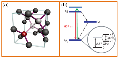
Figure 13: (a) Structure of an NV defect center in the diamond lattice. (b) Energy levels of an NV center in diamond: green, upward arrow for off-resonant optical transitions, red, downward arrow for fluorescence, and dashed arrows for non-radiative, spin-flip decay. Panel (a) is extracted from Ref. Balasubramanian et al. (2009) and panel (b) is reproduced from Ref. Maze et al. (2008b).

VIII Microscopic quantum many-body theories

In previous sections, we have described the central spin decoherence in a quantum bath using a generic pure dephasing Hamiltonian [Eq. (43)]. In this section, we focus on the most relevant issue in quantum computing: the decoherence of a central electron spin in a nanoscale nuclear spin bath in semiconductor nanostructures, such as quantum dots, donors in silicon, and diamond NV centers. First we give the microscopic Hamiltonian relevant for these systems.

VIII.1 Microscopic model

Under moderate to strong external magnetic field (whose axis is defined as the $z$ axis), the non-secular terms of the HFI between the electron spin and various intrinsic nuclear spin interactions (as discussed in Sec. VII.1.3) are suppressed. The total Hamiltonian includes the electron Zeeman term $\hat{H}_{0}\equiv\omega_{0}\hat{S}_{z}$, the nuclear Zeeman term (for simplicity, we consider one nuclear spin species with spin $I$ and gyromagnetic ratio $\gamma_{I}$)

$$\hat{H}_{Z}\equiv-\gamma_{I}B\sum_{j}\hat{I}_{j}^{z}\equiv\omega_{I}\sum_{j}\hat{I}_{j}^{z},$$

the secular part $\hat{S}_{z}\sum_{i}a_{i}\hat{I}_{i}^{z}\equiv\hat{S}_{z}\hat{h}_{z}$ of the HFI ($a_{i}$ is the HFI coefficient and $\hat{h}_{z}$ is widely known as the nuclear Overhauser field), the diagonal part

$$\hat{H}_{\mathrm{d}}\equiv\frac{1}{2}\sum_{i\neq j}\lambda_{ij}^{\mathrm{d}}\hat{I}_{i}^{z}\hat{I}_{j}^{z}$$ (52)

and pair-wise flip-flops part

$$\hat{H}_{\mathrm{ff}}\equiv\sum_{i\neq j}\lambda_{ij}^{\mathrm{ff}}\hat{I}_{i}^{+}\hat{I}_{j}^{-}$$ (53)

of intrinsic nuclear spin interactions, and electron-mediated nuclear spin flip-flop term $2\hat{S}_{z}\tilde{H}_{\mathrm{ff}}$, where Yao et al. (2006); Liu et al. (2007); Yao et al. (2007); Cywiński et al. (2009b)

$$\tilde{H}_{\mathrm{ff}}=\frac{\hat{h}_{x}^{2}+\hat{h}_{y}^{2}}{4\omega_{0}}\approx\sum_{i\neq j}\frac{a_{i}a_{j}}{4\omega_{0}}\hat{I}_{i}^{+}\hat{I}_{j}^{-}\equiv\sum_{i\neq j}\tilde{\lambda}_{ij}^{\mathrm{ff}}\hat{I}_{i}^{+}\hat{I}_{j}^{-},$$ (54)

$\hat{h}_{x}$, $\hat{h}_{y}$ are the transverse parts of $\mathbf{\hat{h}}\equiv\sum_{i}a_{i}\mathbf{\hat{I}}_{i}$ and in the approximation we have neglected a small correction $\sim\sum_{i}a_{i}^{2}/\omega_{0}$ to the electron Zeeman splitting. In the interaction picture with respect to $\hat{H}_{0}+\hat{H}_{Z}$, the total Hamiltonian assumes the standard pure dephasing form (Eq. (43)), where Yao et al. (2006); Liu et al. (2007); Yao et al. (2007)

$$\hat{H}_{\pm} =\hat{H}_{\mathrm{d}}+\hat{H}_{\mathrm{ff}}\pm\frac{1}{2}(2\tilde{H}_{\mathrm{ff}}+\hat{h}_{z})$$ (55a)

$$=\pm\sum_{j}\frac{a_{j}}{2}\hat{I}_{j}^{z}+\frac{1}{2}\sum_{i\neq j}\lambda_{ij}^{\mathrm{d}}\hat{I}_{i}^{z}\hat{I}_{j}^{z}+\sum_{i\neq j}(\lambda_{ij}^{\mathrm{ff}}\pm\tilde{\lambda}_{ij}^{\mathrm{ff}})\hat{I}_{i}^{+}\hat{I}_{j}^{-}.$$ (55b)

This corresponds to $$\hat{H}_{B}\equiv\hat{H}_{\mathrm{d}}+\hat{H}_{\mathrm{ff}} \hat{b}\equiv 2\tilde{H}_{\mathrm{ff}}+\hat{h}_{z} \{a_{i}\} \lambda_{ij}^{\mathrm{d}},\lambda_{ij}^{\mathrm{ff}},\tilde{\lambda}_{ij}^{\mathrm{ff}} \lambda_{ij}^{\mathrm{d}},\lambda_{ij}^{\mathrm{ff}} \tilde{\lambda}_{ij}^{\mathrm{ff}}$$ and . As listed in Table 2, the HFI are much larger than various nuclear spin interactions . Also note that the intrinsic nuclear spin interactions are local, i.e., negligible between distant nuclear spins, while the electron-mediated nuclear spin interactions are non-local.

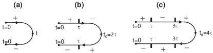
Figure 14: Contour modulation function for different DD sequences: (a) FID, (b) Hahn echo, and (c) CPMG-2.

The initial state of the nuclear spin bath is the therml state $\hat{\rho}_{B}^{\mathrm{eq}}\propto\hat{I}$ [Eq. (33)], which is maximally mixed even at very low temperature (e.g., a few Kelvins) due to the small nuclear Zeeman splitting. Choosing a different initial state of the bath will change the thermal noise and hence inhomogeneous dephasing, but usually does not influence the “true” decoherence due to the quantum noise. For “true” decoherence, sometimes we may take the initial state of the bath as a pure product state

$$|J\rangle=\otimes_{j}|m_{j}\rangle$$ (56)

of the Zeeman eigenstate of each bath spin ($\hat{I}_{j}^{z}|m_{j}\rangle=m_{j}|m_{j}\rangle$). The central spin decoherence can be written as an integral over the contour $\mathrm{C}$: $0\rightarrow t_{\mathrm{d}}\rightarrow 0$:

$$L(t_{\mathrm{d}})=\langle\mathcal{T}_{\mathrm{C}}e^{-i\int_{\mathrm{C}}\hat{H}(z)dz}\rangle,$$ (57)

where $\langle\cdots\rangle\equiv\langle J|\cdots|J\rangle$ for a pure initial state or $\langle\cdots\rangle\equiv\operatorname*{Tr}[\hat{\rho}_{B}^{\mathrm{eq}}(\cdots)]$ for a thermal initial state,

$$\hat{H}(z)=\sum_{j}\omega_{j}(z)\hat{I}_{j}^{z}+\frac{1}{2}\sum_{i\neq j}\lambda_{ij}^{\mathrm{d}}(z)\hat{I}_{i}^{z}\hat{I}_{j}^{z}+\sum_{i\neq j}\lambda_{ij}^{\mathrm{ff}}(z)\hat{I}_{i}^{+}\hat{I}_{j}^{-}$$ (58)

is the bath Hamiltonian on the contour, $\omega_{j}(z)\equiv a_{j}s(z)/2$, $\lambda_{ij}^{\mathrm{ff}}(z)\equiv\lambda_{ij}^{\mathrm{ff}}+s(z)\tilde{\lambda}_{ij}^{\mathrm{ff}}$, $\lambda_{ij}^{\mathrm{d}}(z)\equiv\lambda_{ij}^{\mathrm{d}}$, and $s(z)$ is the DD modulation function on the contour $\mathrm{C}$: it start from $+1$ and switch its sign whenever the central spin is flipped or at $t_{\mathrm{d}}$. FID corresponds to $s(z)\equiv+1$ on the upper branch and $s(z)\equiv-1$ on the lower branch. Some examples of $s(z)$ are shown in Fig. 14. For an arbitrary function $f(z)\equiv f_{+}(t)$ ($z\in$ upper branch) or $f_{-}(t)$ ($z\in$ lower branch), the contour integral is defined as $\int_{\mathrm{C}}f(z)dz\equiv\int_{0}^{t_{\mathrm{d}}}f_{+}(t)dt+\int_{t_{\mathrm{d}}}^{0}f_{-}(t)dt$.

VIII.2 Noises from spin bath dynamics: general considerations

The central spin decoherence is the product of inhomogeneous dephasing due to the thermal noise and “true” decoherence due to the quantum noise (see Sec. V.2). The former usually dominates the FID, but is completely removed by any DD at the echo time, so only the quantum noise, which is usually independent of the initial state of the bath, contributes to central spin decoherence under DD.

VIII.2.1 Thermal noise

On the time scale of inhomogeneous dephasing, nuclear spin interactions $\hat{H}_{\mathrm{d}},$ $\hat{H}_{\mathrm{ff}}$, $\tilde{H}_{\mathrm{ff}}$ can be neglected and $L(t)\equiv\langle e^{-i\hat{h}_{z}t}\rangle$. For a sufficiently large number of nuclear spins, $\hat{h}_{z}$ as the sum of many independent random variables obeys the Gaussian statistics. This gives the Gaussian inhomogeneous dephasing [cf. Eq. (9)]

$$L_{\mathrm{inh}}(t)=e^{-(h_{\mathrm{rms}}t)^{2}/2}\equiv e^{-t^{2}/(T_{2}^{\ast})^{2}}$$ (59)

on a time scale

$$T_{2}^{\ast}=\frac{\sqrt{2}}{h_{\mathrm{rms}}}$$

with

$$h_{\mathrm{rms}}^{2}\equiv\langle\hat{h}_{z}^{2}\rangle=\frac{I(I+1)}{3}\sum_{i}a_{i}^{2},$$

which is insensitive to the specific distribution of $\{a_{i}\}$. From Table I, the typical inhomogeneous dephasing time is estimated as $T_{2}^{\ast}\sim$ a few nanoseconds for a QD containing $N\sim 10^{4}$-$10^{6}$ nuclei Yao et al. (2006); Liu et al. (2007); Yao et al. (2007).

VIII.2.2 Quantum noises from nuclear spin clusters

Quantum noises are determined by the quantum fluctuations of the baths. According to Eq. (55), the elementary excitations of the bath are flip-flops of bath spin pairs. On a short time scale, the flip-flops of different pairs are nearly independent. On a longer time scale, the successive flip-flop of different pairs involving a common bath spin generates correlated fluctuation of larger and larger clusters. When central spin decoherence time is relatively long (e.g., for a small ¹³C nuclear spin bath in diamond NV centers), or when the correlated fluctuation of small clusters are reduced by DD control, the correlated fluctuations of larger clusters become important.

In recent years, microscopic quantum many-body theories have been developed to quantitatively describe the correlated fluctuations of nuclear spin clusters and the induced electron spin decoherence in nanoscale nuclear spin baths. The pair-correlation approximation Yao et al. (2006); Liu et al. (2007); Yao et al. (2007) and density matrix cluster expansion Witzel et al. (2005); Witzel and Das Sarma (2006) are the two first quantum many-body theories, which have been independently developed and are equivalent in the leading order. The former treated the flip-flop of different pairs as independent and provides a transparent physical picture for central spin decoherence, but neglects the correlated fluctuation of larger clusters. The latter provides a convenient way to include the leading-order effect of correlated fluctuation of larger clusters, but may not converge to the exact results for relatively small baths. The subsequent theory, the linked-cluster expansion (LCE) Saikin et al. (2007), accurately accounts for the fluctuations due to successively higher-order interactions among the nuclear spins through Feynman diagrams of successively higher order, but becomes increasingly inefficient at higher orders and may not converge for a relatively small spin bath. When each nuclear spin is coupled to all the other nuclear spins [see Eq. (54) for an example], a large-$N$ expansion ($N$ is the number of nuclear spins) of LCE is possible (so-called ring diagram approximation Cywiński et al. (2009b, a); Cywinski et al. (2010)), which turns out to be equivalent to the semi-classical noise model Bluhm et al. (2011); Neder et al. (2011). For a simple and accurate account for the correlated fluctuation of large clusters, the cluster-correlation expansion (CCE) has been developed Yang and Liu (2008b, 2009), which covers the validity ranges of previous theories, produces the exact results even for relatively small baths, and has successfully predicted and explained a series of experimental results for various solid state systems.

In the following subsections, we will review these many-body theories. First we introduce the LCE, which accounts for various fluctuation processes through Feynman diagrams. Then we introduce the ring diagram approximation as a partial summation of an infinite number of certain Feynman diagrams. Next CCE is introduced as an expansion method corresponding to an infinite summation of all the Feynman diagrams. Finally, we will give a conceptual understanding of CCE as a systematic method to treat the correlated fluctuation of larger spin clusters in a canonical quantum spin system (while the cluster expansion and disjoint cluster approximation Maze et al. (2008a); Hall et al. (2014) can be regarded as certain approximations to the CCE), thus it can be used to calculate not only central spin decoherence but also other quantities such as the quantum noise spectrum of the spin bath.

Before discussing the different many-body theories, we emphasize that in cluster expansion and CCE the term “cluster” refers to a group of physical bath spins, e.g., a three-spin cluster contains three different bath spins. The “linked-cluster expansion” (LCE) is a diagrammatic expansion with respect to the number of interaction lines in a Feynman diagram, e.g., a third-order Feynman diagram contains three interactions lines, but not necessarily contain three different bath spins. By contrast, the CCE theory and the cluster expansion theory are expansions with respect to the number of bath spins, e.g., a three-spin cluster contains three different bath spins. Nevertheless, there is a close connection between the number of bath spins contained in a cluster and the order of Feynman diagrams. This allows us to establish a connection between the CCE and the LCE (to be discussed shortly).

VIII.3 Linked-cluster expansion

Linked-cluster expansion (LCE) is a standard many-body technique to evaluate the average of a general time-ordered exponential, as defined by its Taylor expansion:

$$\langle\mathcal{T}_{\mathrm{C}}e^{-i\int_{\mathrm{C}}\hat{O}(z)dz}\rangle$$

$$\equiv\sum_{n=0}^{\infty}\frac{(-i)^{n}}{n!}\int_{\mathrm{C}}dz_{1}\cdots\int_{\mathrm{C}}dz_{n}\langle\mathcal{T}_{\mathrm{C}}[\hat{O}(z_{1})\cdots\hat{O}(z_{n})]\rangle,$$ (60)

where the average $\langle\cdots\rangle$ is carried out over a non-interacting ensemble of bosons, fermions, or spin systems Saikin et al. (2007), and $\hat{O}(z)$ consists of bosonic (or fermionic) field operators or spin operators in the interaction picture. An example is the contour Hamiltonian in Eq. (58), where the spin operators in the interaction picture are $\hat{I}_{i}^{z}(z)\equiv\hat{I}_{i}^{z}$ and $\hat{I}_{i}^{\pm}(z)\equiv\hat{I}_{i}^{\pm}$.

LCE dictates that the expansion in Eq. (60) can be reduced to an exponential function of linked diagrams - hence the name of LCE. When $\hat{O}(z)=\tilde{\varphi}$ is a classical Gaussian random variable or when $\hat{O}(z)=\sum_{m}(\alpha_{m}\hat{c}_{m}+\beta_{m}\hat{c}_{m}^{\dagger})$ is a bosonic field operator, there is only one linked diagram corresponding to $(-1/2)\langle\tilde{\varphi}^{2}\rangle$ or $(-1/2)\langle\hat{O}^{2}\rangle$, so LCE reduces to Eq. (12) or Eq. (40). Here we introduce the LCE for spin baths relevant for central spin decoherence in nuclear spin baths, thus the average $\langle\cdots\rangle\equiv\operatorname*{Tr}[\hat{\rho}_{\mathrm{NI}}(\cdots)]$ refers to a non-interacting spin bath state

$$\hat{\rho}_{\mathrm{NI}} =\frac{e^{-\beta\hat{H}_{\mathrm{NI}}}}{\operatorname*{Tr}e^{-\beta\hat{H}_{\mathrm{NI}}}},$$

$$\hat{H}_{\mathrm{NI}} =\sum_{i}\omega_{i}\hat{I}_{i}^{z}.$$

The spin operators in the interaction picture are taken to be $\hat{I}_{i}^{\pm}(z)=e^{\pm i\varepsilon_{i}z}\hat{I}_{i}^{\pm}$ and $\hat{I}_{i}^{z}(z)=\hat{I}_{i}^{z}$, where in general $\varepsilon_{i}$ could be different from $\omega_{i}$.

VIII.3.1 LCE for spin baths

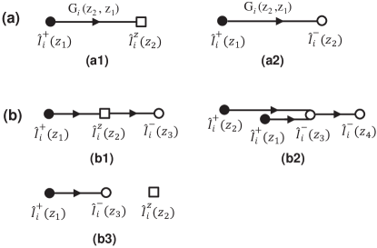
Figure 15: Diagrammatic representation of the contraction of (a) two and (b) three spin operators. The spin operators $\hat{I}_{+},$ $\hat{I}_{-}$, and $\hat{I}_{z}$ correspond to a filled circle, an empty circle, and an empty square.

The first key ingredient of LCE for a spin bath is the concept of contraction Vaks et al. (1968), defined between a spin raising operator $\hat{I}_{i}^{+}(z_{1})$ and an arbitrary spin operator $\hat{I}_{j}^{\alpha}(z_{2})$ in the interaction picture:

$$[\hat{I}_{j}^{\alpha}(z_{2})]^{\bullet}[\hat{I}_{i}^{+}(z_{1})]^{\bullet} \equiv[\hat{I}_{i}^{+}(z_{1})]^{\bullet}[\hat{I}_{j}^{\alpha}(z_{2})]^{\bullet}$$

$$\equiv\delta_{i,j}G_{i}(z_{2},z_{1})e^{i\varepsilon_{i}(z_{1}-z_{2})}[\hat{I}_{j}^{\alpha},\hat{I}_{i}^{+}](z_{2}).$$ (61)

where $z$ is the time on the contour $\mathrm{C}$, $G_{i}(z_{2},z_{1})=\theta(z_{2}-z_{1})[1+\bar{n}(\omega_{i})]+\theta(z_{1}-z_{2})\bar{n}(\omega_{i})$ is the contour Green’s function, $\theta(z)$ is the Heaviside step function on the contour, and $\bar{n}(\omega)\equiv 1/(e^{\beta\omega}-1)$ is the Bose-Einstein distribution function. The contraction can be visualized by Feynman diagrams as sketched in Fig. 15(a). The contraction of $\hat{I}_{i}^{+}(z_{1})$ and $\hat{I}_{i}^{\alpha}(z_{2})$ is represented by an arrow going from $\hat{I}_{i}^{+}(z_{1})$ to $\hat{I}_{i}^{\alpha}(z_{2})$: the arrow itself represents $e^{i\varepsilon_{i}(z_{1}-z_{2})}G_{i}(z_{2},z_{1})$, while the commutator $[\hat{I}_{i}^{+},\hat{I}_{i}^{\alpha}](z_{\alpha})$ is to be taken at the end of the arrow. Since $[\hat{I}_{z},\hat{I}_{+}]=\hat{I}_{+}$ and $[\hat{I}_{-},\hat{I}_{+}]=-2\hat{I}_{z}$, the contraction of $\hat{I}_{i}^{+}(z_{1})$ and $\hat{I}_{i}^{z}(z_{2})$ [or $\hat{I}_{i}^{-}(z_{2})$] eliminates $\hat{I}_{i}^{+}(z_{1})$ and converts $\hat{I}_{i}^{z}(z_{2})$ [or $\hat{I}_{i}^{-}(z_{2})$] to $\hat{I}_{i}^{+}(z_{2})$ [or $-2\hat{I}_{i}^{z}(z_{2})$], reducing the number of spin operators by one. Note that the contraction of spin operators is quite different from the contraction of bosonic or fermionic field operators: the latter is just a c-number, while the former is still a spin operator that should be used in subsequent contractions. For example, as shown in Fig. 15(b1), the contraction of $\hat{I}_{i}^{+}(z_{1})$ and $\hat{I}_{i}^{z}(z_{2})$ produces $\hat{I}_{i}^{+}(z_{2})$, which in turn contracts with $\hat{I}_{i}^{-}(z_{3})$ and produces $(-2)\hat{I}_{i}^{z}(z_{3})$. Another example is shown in Fig. 15(b2): the contraction of $\hat{I}_{i}^{+}(z_{1})$ [or $\hat{I}_{i}^{+}(z_{2})$] and $\hat{I}_{i}^{-}(z_{3})$ produces $(-2)\hat{I}_{i}^{z}(z_{3})$, then $\hat{I}_{i}^{z}(z_{3})$ contracts with $\hat{I}_{i}^{+}(z_{2})$ [or $\hat{I}_{i}^{+}(z_{1})$] to produce $\hat{I}_{i}^{+}(z_{3})$, which in turn contracts with $\hat{I}_{i}^{-}(z_{4})$ to produce $(-2)\hat{I}_{i}^{z}(z_{4})$. Here the order of the contraction does not change the result.

The second key ingredient is the Wick’s theorem for spin operators Vaks et al. (1968); Yang and Wang (1974); Saikin et al. (2007); Yang and Liu (2008b); Ma et al. (2014). Lets consider an arbitrary contour time-ordered product of spin operators in the interaction picture (spin operators commute inside the $\mathcal{T}_{\mathrm{C}}$ product)

$$\langle\mathcal{T}_{\mathrm{C}}[\hat{I}_{i}^{\alpha}(z_{1})\cdots\hat{I}_{k}^{\gamma}(z_{n})]\rangle=\operatorname*{Tr}\{\hat{\rho}_{\mathrm{NI}}\mathcal{T}_{\mathrm{C}}[\hat{I}_{i}^{\alpha}(z_{1})\cdots\hat{I}_{k}^{\gamma}(z_{n})]\}.$$ (62)

Wick’s theorem states that the contour time-ordered product of spin operators $\mathcal{T}_{\mathrm{C}}[\cdots]$ in Eq. (62) can be replaced by the sum of all possible fully contracted products containing only $\hat{I}_{z}$ operators. If $\mathcal{T}_{\mathrm{C}}[\cdots]$ contains different numbers of $\hat{I}_{+}$ and $\hat{I}_{-}$ operators, then Eq. (62) vanishes. For example, the diagram in Fig. 15(a1) vanishes since it only contains one $\hat{I}_{+}$ operator but no $\hat{I}_{-}$ operator, while all the other diagrams in Fig. 15 containing equal numbers of $\hat{I}_{+}$ and $\hat{I}_{-}$ operators are fully contracted products. As another example, $\mathcal{T}_{\mathrm{C}}[\hat{I}_{i}^{+}(z_{1})\hat{I}_{i}^{z}(z_{2})\hat{I}_{i}^{-}(z_{3})]$ has two possible fully contracted products: a connected diagram $([\hat{I}_{i}^{+}(z_{1})]^{\bullet}[\hat{I}_{i}^{z}(z_{2})]^{\bullet})^{\circ}(\hat{I}_{i}^{-}(z_{3}))^{\circ}$[Fig. 15(b1)] and a disconnected diagram $[\hat{I}_{i}^{+}(z_{1})]^{\bullet}[\hat{I}_{i}^{-}(z_{3})]^{\bullet}\times\hat{I}_{i}^{z}(z)$ [Fig. 15(b3)].

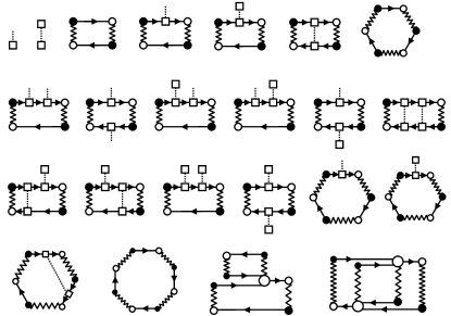
Figure 16: Topologically inequivalent connected diagrams up to the 4th order for the Hamiltonian in Eq. (58). Here dotted lines connected to a single empty square denote $\omega_{j}(z)$, dotted lines connected to two empty squares denotes $\lambda_{ij}^{\mathrm{d}}(z)$, and wavy lines denote $\lambda_{ij}^{\mathrm{ff}}(z)$, e.g., the first (second) diagram represents the first (second) term of $\hat{H}(z)$. Reproduced from Ref. Yang and Liu (2008b).

By appling Wick theorem to each $\mathcal{T}_{\mathrm{C}}$ product, Eq. (60) can be decomposed as the sum of fully contracted products or equivalently diagrams, including connected ones and disconnected ones. The LCE theorem states that all these diagrams can be resummed into an exponential form Abrikosov et al. (1963):

$$\langle\mathcal{T}_{\mathrm{C}}e^{-i\int_{\mathrm{C}}\hat{O}(z)dz}\rangle=\langle e^{\hat{\pi}}\rangle,$$ (63)

where $\hat{\pi}$ represents the sum of all the connected diagrams contained in Eq. (60). Taking the contour bath Hamiltonian in Eq. (58) as an example, all the topologically inequivalent connected diagrams up to the 4th order of the bath interactions are shown in Fig. 16.

For a spin-1/2 bath, the average $\left\langle J\left|\cdots\right|J\right\rangle$ over a pure product state $|J\rangle$ [Eq. (56)] (an eigenstates of $\hat{H}_{\mathrm{NI}}$) can be taken as the average over an zero-temperature ensemble $\operatorname*{Tr}[\hat{\rho}_{\mathrm{NI}}\cdots]$, with $\omega_{i}<0$ (or $>0$) for $\left|m_{i}\right\rangle=\left|\uparrow\right\rangle$ (or $\left|\downarrow\right\rangle$). Therefore the “true” decoherence caused by a bath in the pure state $|J\rangle$ can be written as Saikin et al. (2007); Yang and Liu (2008b); Ma et al. (2014):

$$L(t_{\mathrm{d}})=\langle J|\mathcal{T}_{\mathrm{C}}e^{-i\int_{\mathrm{C}}\hat{H}(z)dz}|J\rangle=e^{\pi},$$ (64)

where

$$\pi\equiv\langle J|\hat{\pi}|J\rangle=\langle J|\mathcal{T}_{\mathrm{C}}e^{-i\int_{\mathrm{C}}\hat{H}(z)dz}|J\rangle_{\mathrm{connected}}$$ (65)

is the sum of all connected Feynman diagrams contained in $\langle J|\mathcal{T}_{\mathrm{C}}e^{-i\int_{\mathrm{C}}\hat{H}(z)dz}|J\rangle$. Here each constituent diagram of $\pi$ is a c-number, obtained from the constituent diagram of $\hat{\pi}$ by replacing $\hat{I}_{i}^{z}$ with $\langle J|\hat{I}_{i}^{z}|J\rangle=m_{i}$. When bath spins are higher than 1/2, the average $\left\langle J\left|\cdots\right|J\right\rangle$ over a pure product state $|J\rangle$ [Eq. (56)] can still be taken as an zero-temperature ensemble $\operatorname*{Tr}[\hat{\rho}_{\mathrm{NI}}\cdots]$ as long as each bath spin is mapped to a composite of pseudo-spin-1/2’s Yang and Liu (2008b).

The LCE has been applied to the phosphorus donor electron spin in a ²⁹Si nuclear spin bath Saikin et al. (2007); Ma et al. (2014). The connected Feynman diagrams have been evaluated up to the fourth order of the bath interactions. The results agree reasonably with the experimental data Tyryshkin et al. (2006). The FID is dominated by the leading-order flip-flop process of nuclear spin pairs (the third diagram in Fig. 16). Under higher-order DD, it is necessary to take higher-order diagrams into account, but the tedious diagram counting and evaluation makes it difficult to go to very high orders.

VIII.3.2 Ring diagram approximation

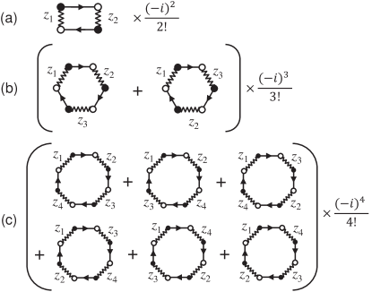
Figure 17: Ring diagrams containing up to (a) two, (b) three, and (c) four nucelar spins.

The difficulty in counting and evaluating higher-order Feynman diagrams in LCE could be greatly simplified under a relatively weak magnetic field Cywiński et al. (2009b, a); Cywinski et al. (2010), where the electron-mediated nuclear spin interactions $\tilde{\lambda}_{ij}^{\mathrm{ff}}$ dominates over the intrinsic interactions $\lambda_{ij}^{\mathrm{ff}}$ and $\lambda_{ij}^{\mathrm{d}}$. In this case $\lambda_{ij}^{\mathrm{ff}}$ and $\lambda_{ij}^{\mathrm{d}}$ in Eq. (58) can be dropped, the total Hamiltonian becomes $\hat{H}=\hat{S}_{z}\hat{b}$ with $\hat{b}\equiv\hat{h}_{z}+2\tilde{H}_{\mathrm{ff}}$ [Eq. (54)], and the decoherence $L(t_{\mathrm{d}})=\langle e^{-i\hat{b}\int_{0}^{t_{\mathrm{d}}}s(t)dt}\rangle$ [cf. Eq. (57)] is completely removed by any DD at the echo time (in this case decoherence comes from the flip-flop between nuclei of different species Cywiński et al. (2009b, a); Cywinski et al. (2010)). The “true” decoherence due to quantum noises in FID Cywiński et al. (2009b, a); Cywinski et al. (2010),

$$L_{\mathrm{dyn}}(t)=\langle J|e^{-i\hat{b}t}|J\rangle=\langle J|\mathcal{T}e^{-2i\int_{0}^{t}\tilde{H}_{\mathrm{ff}}(t^{\prime})dt^{\prime}}|J\rangle\approx\langle\mathcal{T}e^{-2i\int_{0}^{t}\tilde{H}_{\mathrm{ff}}(t^{\prime})dt^{\prime}}\rangle$$

is described by the simplified “contour” Hamiltonian

$$\tilde{H}_{\mathrm{ff}}(t)=\sum_{i\neq j}\tilde{\lambda}_{ij}^{\mathrm{ff}}\hat{I}_{i}^{+}\hat{I}_{j}^{-}e^{i(a_{i}-a_{j})t/2},$$

thus all the Feynman diagrams (Fig. 16) involving $\lambda_{ij}^{\mathrm{d}}(z)$ and $\omega_{j}(z)$ vanish. Since each nuclear spin couples to all the other nuclear spins with comparable strength, the value of a Feynman diagram involving $m$ different nuclear spins is of the order $O(N^{m}$) with $N$ being the number of nuclear spins. This enables a leading-order expansion with respect to $1/N$ Saikin et al. (2007); Cywiński et al. (2009b, a); Cywinski et al. (2010): among all the Feynman diagrams containing the same number of interaction lines, it suffices to keep only those diagrams involving the maximal number of nuclear spins, i.e. all the ring diagrams contained in $\langle\mathcal{T}e^{-2i\int_{0}^{t}\tilde{H}_{\mathrm{ff}}(t^{\prime})dt^{\prime}}\rangle$ (Fig. 17). This is the ring diagram approximation Cywiński et al. (2009b, a); Cywinski et al. (2010). For $t\ll$ inverse HFI, it gives a power-law decay

$$L_{\mathrm{dyn}}(t)\approx\frac{1}{1+it/T_{\mathrm{dyn}}},$$ (66)

which is insensitive to the specific distribution of the HFI coefficients $\{a_{i}\}$, on a time-scale

$$T_{\mathrm{dyn}}\equiv\frac{\omega_{0}}{h_{\mathrm{rms}}^{2}}.$$ (67)

For $t\gg T_{\mathrm{dyn}}$, the denominator $1+it/T_{\mathrm{dyn}}\approx it/T_{\mathrm{dyn}}$ gives rise to a $\pi/2$ phase shift of the electron Larmor precession. Power-law behavior and a long-time $\pi/4$ phase shift has also been observed in the single-spin Rabi oscillation decay Koppens et al. (2007); Hanson et al. (2008). For long times $t\gg$ inverse HFI, it gives an exponential decay Liu et al. (2007); Coish et al. (2008) on a time scale that depends sensitively on the distribution of $\{a_{i}\}$. The relevance of the power-law decay and the exponential decay depends on the magnetic field. For weak fields such that $T_{\mathrm{dyn}}\ll$ inverse HFI, most of the coherence decay follows the short-time power-law behavior in Eq. (66). By contrast, in the opposite limit $T_{\mathrm{dyn}}\gg$ inverse HFI, most of the coherence decays exponentially. Under spin echo, the calculated decoherence under weak magnetic fields agrees with the experiment in gated GaAs QDs Koppens et al. (2008). At slightly stronger magnetic fields, characteristic oscillations with frequencies equal to the differences of the nuclear Zeeman frequencies of different nuclear species is predicted Cywiński et al. (2009a, b) and subsequently observed experimentally Bluhm et al. (2011).

Essentially, the ring diagram approximation assumes that all the spin operators in $\tilde{H}_{\mathrm{ff}}(z)$ commute with each other Cywiński et al. (2009b, a). This involves an $O(1/N)$ error Barnes et al. (2011) and is equivalent to a semi-classical treatment of the quantum noise. A detailed discussion can be found in Ref. Neder et al. (2011) and Cywinski (2011). Taking the “true” decoherence in the FID as an example, on a time scale $t\ll$ inverse HFI,

$$L_{\mathrm{dyn}}(t)=\langle e^{-2i{\tilde{H}}_{\mathrm{ff}}t}\rangle=\langle e^{-i(\hat{h}_{x}^{2}+\hat{h}_{y}^{2})t/(2\omega_{0})}\rangle.$$

Regarding ${\hat{h}}_{x}$ and ${\hat{h}}_{y}$ as independent, classical quasi-static Gaussian noise obeying the distribution $P(h)=e^{-h^{2}/(2h_{\mathrm{rms}}^{2})}/(\sqrt{2\pi}h_{\mathrm{rms}})$ gives

$$L_{\mathrm{dyn}}(t)\approx\int P(h_{x})dh_{x}\int P(h_{y})dh_{y}\ e^{-i({h}_{x}^{2}+{h}_{y}^{2})t/(2\omega_{0})},$$

which reproduces Eqs. (66) and (67).

VIII.4 Cluster-correlation expansion

The key idea of CCE is to factorize Eq. (57) into the product of cluster-correlation terms, each of which accounting for the irreducible, correlated fluctuations in a given bath spin cluster. For a finite-time evolution as in the central spin decoherence problem, a convergent result is obtained by truncating the expansion up to a certain cluster size. The two-spin cluster truncation of the CCE corresponds to the pair-correlation approximation Yao et al. (2006); Liu et al. (2007); Yao et al. (2007). When the central spin decoherence comes from the contribution of a large number of cluster correlation terms and the contribution from each individual term is small, as the usual case for relatively large baths, CCE coincides with the cluster expansion Witzel et al. (2005); Witzel and Das Sarma (2006). For small baths, however, central spin decoherence may be dominated by the coherent dynamics of a few cluster correlation terms. In this case, CCE converges to the exact results while the cluster expansion does not.

CCE has been applied to electron spin decoherence for phosphorus donor in silicon (Si:P) Witzel et al. (2010), bismuth donors in silicon (Si:Bi) George et al. (2010); Balian et al. (2012); Morley et al. (2013), radical spins in malonic acid crystals Du et al. (2009), and diamond NV center Zhao et al. (2012b). The calculated results agree well with the experimental data, including the decoherence time scale, the temporal profile, and its dependence on the magnetic field. The CCE also provides convincing theoretical demonstrations of atomic-scale sensing of distant nuclear spin clusters Zhao et al. (2011a) and anomalous decoherence effects Zhao et al. (2011b). Both effects have been observed subsequently Huang et al. (2011); Shi et al. (2014) and these experiments are well explained by CCE calculations.

CCE can be understood in two different viewpoints. First, CCE is a re-grouping and infinite summation of all the LCE diagrams Yang and Liu (2008b). Second, CCE is a systematic method to treat the irreducible, correlated fluctuation of successively larger spin clusters in a canonical ensemble, so CCE can also be used to calculate other quantities such as the quantum noise spectrum. The first understanding applies to a pure product state $|J\rangle$ of the bath [Eq. (56)]. The second understanding leads to two formulations: CCE for a general non-interacting bath state has a simpler form Yang and Liu (2009), but CCE for a pure product state of a general spin bath has better convergence Yang and Liu (2008b).

VIII.4.1 CCE as infinite summation of LCE diagrams

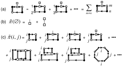
Figure 18: (a) Expansion of a third-order connected diagram into diagrams involving the flip-flops of different clusters of spins. (b) and (c) show the diagrams contained in $\tilde{\pi}(\varnothing)$ and $\tilde{\pi}(i,j)$, respectively. Reproduced from Ref. Yang and Liu (2008b).

For a pure product state $|J\rangle$ [Eq. (56)] of the spin bath, the connection between LCE [Eqs. (64) and (65)] to CCE is based on the observation that each connected LCE diagram can be expanded as the sum of diagrams involving the flip-flops of different clusters of spins. As an example shown in Fig. 18(a) for a spin-1/2 bath, a third-order LCE diagram involving the flip-flop of a spin pair contains diagrams for spin clusters $(1,2)$, $(1,3)$, $\cdots$, where the numbers stand for the indices of the spins that have been flipped. Thus all the connected diagrams can be classified according to the spin clusters instead of the interaction orders. For an arbitrary (empty or non-empty) cluster $\mathcal{C}$, we define the cluster-correlation term $\tilde{\pi}({\mathcal{C}})$ as the sum of all connected diagrams in which all and only the spins in cluster $\mathcal{C}$ have been flipped. For instance, some of the diagrams constituting $\tilde{\pi}(\varnothing)$ and $\tilde{\pi}(i,j)$ for a spin-1/2 Hamiltonian in Eq. (58) are shown in Figs. 18(b) and 18(c), respectively.

With these $\{\tilde{\pi}\}$ functions, the exact LCE is expressed as

$$\pi=\sum\limits_{\mathcal{C}\subseteq\{1,2,\cdots,N\}}\tilde{\pi}\left({\mathcal{C}}\right),$$ (68)

i.e., the sum of cluster-correlation terms for all spin clusters (including the empty cluster $\varnothing$) in the $N$-spin bath. In particular, the infinite summation of all the connected diagrams for a certain cluster ${\mathcal{C}}$ and all its subsets

$$\pi\left({\mathcal{C}}\right)\equiv\sum_{{\mathcal{C}}^{\prime}\subseteq{\mathcal{C}}}\tilde{\pi}\left({\mathcal{C}}^{\prime}\right),$$ (69)

is just equal to $\pi$ [Eq. (65)] with all the terms involving the flip-flop of spins outside the cluster ${\mathcal{C}}$ dropped, or, equivalently, with the bath Hamiltonian $\hat{H}(z)=\hat{H}(\hat{\mathbf{I}}_{1},\cdots,\hat{\mathbf{I}}_{N})$ replaced with $H(\{\hat{\mathbf{I}}_{j\in\mathcal{C}}\},\{\langle J|\hat{\mathbf{I}}_{j\notin\mathcal{C}}|J\rangle\})$ in which the spins outside the cluster are mean-field averaged. Thus we have

$$e^{\pi\left({\mathcal{C}}\right)}=\langle J|\mathcal{T}_{\mathrm{C}}e^{-i\int_{\mathrm{C}}\hat{H}(\{\hat{\mathbf{I}}_{j\in\mathcal{C}}\},\{\langle J|\hat{\mathbf{I}}_{j\notin\mathcal{C}}|J\rangle\})dz}|J\rangle.$$ (70)

For small clusters $\mathcal{C}$, the Hamiltonian $\hat{H}(\{\hat{\mathbf{I}}_{j\in\mathcal{C}}\},\{\langle J|\hat{\mathbf{I}}_{j\notin\mathcal{C}}|J\rangle\})$ only contains spin operators inside the cluster $\mathcal{C}$, thus $\pi(\mathcal{C})$ can be calculated from Eq. (70) by direct diagonalization. This, in turn, allows $\{\tilde{\pi}(\mathcal{C})\}$ to be extracted recursively from Eq. (69):

$$\tilde{\pi}(\mathcal{C})=\pi\left({\mathcal{C}}\right)-\sum_{{\mathcal{C}}^{\prime}\subset{\mathcal{C}}}\tilde{\pi}\left({\mathcal{C}}^{\prime}\right),$$ (71)

e.g., $\tilde{\pi}(\varnothing)=\pi(\varnothing)$ and $\tilde{\pi}(i)=\pi\left(i\right)-\tilde{\pi}(\varnothing)$.

For a cluster $\mathcal{C}$ containing $|\mathcal{C}|$ bath spins, each diagram in $\tilde{\pi}(\mathcal{C})$ consists of at least $|\mathcal{C}|$ off-diagonal interaction lines that connect all the spins in cluster $\mathcal{C}$ into a linked cluster (see Fig. 18 for examples), thus $\tilde{\pi}(\mathcal{C})\sim(\lambda_{\mathrm{ff}}t_{\mathrm{d}})^{|\mathcal{C}|}$, where $\lambda_{\mathrm{ff}}$ is the typical value of the off-diagonal interactions $\lambda_{ij}^{\mathrm{ff}}(z)$. On a time scale $t_{\mathrm{d}}\ll$ $1/\lambda_{\mathrm{ff}}$, cluster-correlation terms of large clusters are small, so Eq. (68) can be truncated, e.g., keeping cluster-correlation terms containing up to $M$ bath spins gives the $M$th-order truncated CCE (CCE-$M$ for short):

$$\pi^{(M)}=\sum\limits_{|\mathcal{C}|\leq M}\tilde{\pi}\left({\mathcal{C}}\right)=\tilde{\pi}(\varnothing)+\tilde{\pi}^{(1)}+\cdots+\tilde{\pi}^{(M)},$$

where $\tilde{\pi}^{(M)}\equiv{\textstyle\sum_{|\mathcal{C}|=M}}\tilde{\pi}\left({\mathcal{C}}\right)$ is the total contribution from all $M$-spin cluster-correlation terms. If each bath spin interacts, on average, with $q$ spins, then the number of linked clusters containing $m$ bath spins is $\sim Nq^{m-1}$ and $\tilde{\pi}^{(m)}\sim(N/q)(q\lambda_{\mathrm{ff}}t_{\mathrm{d}})^{m}$. Therefore, a sufficient condition for convergence of CCE is

$$t_{\mathrm{d}}<\frac{1}{q\lambda_{\mathrm{ff}}}.$$ (72)

which is usually much longer than the electron spin decoherence time.

VIII.4.2 CCE without LCE: general non-interacting bath state

The CCE formalism described below can be directly used to calculate the average of a general time-ordered exponential over an arbitrary non-interacting ensemble $\hat{\rho}_{\mathrm{NI}}=\otimes_{i=1}^{N}\hat{\rho}_{i}$ ($\hat{\rho}_{i}$ for the $i$th bath spin), i.e., Eq. (57) with $\hat{H}(z)$ being a general spin bath Hamiltonian [not necessarily Eq. (58)] and $\langle\mathcal{\cdots}\rangle\equiv\operatorname*{Tr}[\hat{\rho}_{\mathrm{NI}}(\cdots)]$. However, for clarity we consider Eq. (57) with $\hat{H}(z)$ given by Eq. (58), but the initial state of the bath is a general non-interacting state $\hat{\rho}_{\mathrm{NI}}$.

The first step is to define the cluster term

$$L(\mathcal{C})\equiv\langle\mathcal{T}_{\mathrm{C}}e^{-i\int_{\mathrm{C}}\hat{H}_{\mathcal{C}}(z)dz}\rangle,$$ (73)

where $\hat{H}_{\mathcal{C}}(z)$ is obtained from $\hat{H}(z)$ by dropping all the bath spins outside cluster $\mathcal{C}$, e.g., $\hat{H}_{\{i\}}(z)=\omega_{i}(z)\hat{I}_{i}^{z}$ and $\hat{H}_{\{i,j\}}(z)=\omega_{i}(z)\hat{I}_{i}^{z}+\omega_{j}(z)\hat{I}_{j}^{z}+\lambda_{ij}^{\mathrm{d}}(z)\hat{I}_{i}^{z}\hat{I}_{j}^{z}+\lambda_{ij}^{\mathrm{ff}}(z)(\hat{I}_{i}^{+}\hat{I}_{j}^{-}+h.c.)$. The key observation is that when a cluster $\mathcal{C}$ can be divided into two subsets $\mathcal{C}_{1}$ and $\mathcal{C}_{2}$ such that $\hat{H}_{\mathcal{C}}(z)$ does not contain any interaction between the two subsets, $L(\mathcal{C})$ is factorizable:$\ L(\mathcal{C})=L(\mathcal{C}_{1})L(\mathcal{C}_{2})$. This allows singling out the irreducible, correlated fluctuations of different clusters by defining a hierarchy of cluster-correlation terms $\{\tilde{L}(\mathcal{C})\}$:

$$\tilde{L}(i) \equiv L(i),$$ (74a)

$$\tilde{L}(i,j) \equiv\frac{L(i,j)}{\tilde{L}(i)\tilde{L}(j)},$$ (74b)

$$\cdots$$

$$\tilde{L}(\mathcal{C}) \equiv\frac{L(\mathcal{C})}{\prod_{\mathcal{C}^{\prime}\subset C}\tilde{L}(\mathcal{C}^{\prime})}.$$ (74c)

The central spin coherence is expressed exactly as the product of all possible cluster-correlation terms:

$$L=\prod_{\mathcal{C}\subseteq\{1,2,\cdots,N\}}\tilde{L}(\mathcal{C})=\left(\prod_{i}L(i)\right)\left(\prod_{i\neq j}\tilde{L}(i,j)\right)\cdots.$$ (75)

Since $\hat{H}(z)$ contains pair-wise interactioins $\lambda_{ij}$ (including $\lambda_{ij}^{\mathrm{d}}$ and $\lambda_{ij}^{\mathrm{ff}}$), the pair-correlation term $\ln\tilde{L}(i,j)$ is at least first order in $\lambda_{ij}t_{\mathrm{d}}$ since $L(i,j)=L(i)L(j)$ and hence $\ln\tilde{L}(i,j)=0$ when $\lambda_{ij}=0$. By mathematical induction, it can be proved that the cluster-correlation term $\ln\tilde{L}(\mathcal{C})$ vanishes if the interactions contained in $\hat{H}_{\mathcal{C}}(z)$ cannot connect all the spins in group $\mathcal{C}$ into a linked cluster. Consequently, in the Taylor expansion of $\ln\tilde{L}(\mathcal{C})$ with respect to the bath interaction times the evolution time $t_{\mathrm{d}}$, the bath interaction coefficients contained in every term must: (i) connect all the spins in group $\mathcal{C}$ into a linked cluster, (ii) ensure that each spin inside cluster $\mathcal{C}$ is flipped an even number ($0$, $2$, $4$, $\cdots$) of times, and, if the initial state of the bath $\hat{\rho}_{\mathrm{NI}}\propto\hat{I}$ is maximally mixed, (iii) ensure that every bath spin inside cluster $\mathcal{C}$ appear an even number ($2,4,6,\cdots$) of times. Condition (i) alone ensures that $\ln\tilde{L}(\mathcal{C})$ is at least $(|\mathcal{C}|-1)$th order, while conditions (ii) and (iii) usually make the order of $\ln\tilde{L}(\mathcal{C})$ even higher.

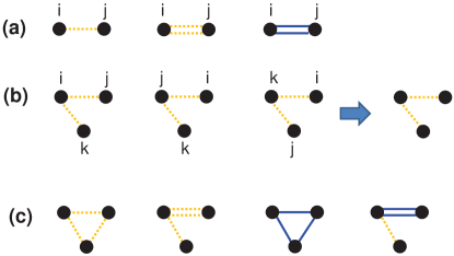
Figure 19: Diagrammatic representation of the lowest-order processes contributing to ensemble cluster-correlation terms for (a) $\tilde{L}(i,j)$ and (b),(c) $\tilde{L}(i,j,k)$. Solid (Dashed) line for off-diagonal (diagonal) spin-spin interaction.

For example, the Taylor expansion of $\ln\tilde{L}(i,j)$ with respect to $\lambda_{ij}^{\mathrm{d}}t_{\mathrm{d}}$ and $\lambda_{ij}^{\mathrm{ff}}t_{\mathrm{d}}$ satisfying conditions (i) and (ii) reads:

$$\ln\tilde{L}(i,j)=c_{1}\lambda_{ij}^{\mathrm{d}}t_{\mathrm{d}}+c_{2}(\lambda_{ij}^{\mathrm{d}}t_{\mathrm{d}})^{2}+c_{3}(\lambda_{ij}^{\mathrm{ff}}t_{\mathrm{d}})^{2}+O(t_{\mathrm{d}}^{3}),$$

as shown diagrammatically in Fig. 19(a). In the first and second terms/diagrams, spin $i$ and spin $j$ are not flipped. In the third term/diagram, each spin is flipped twice. If the initial state of the bath is maximally mixed, then condition (iii) dictates that the first term/diagram vanishes since in this term/diagram each spin only appears once. In this case, the leading Taylor expansion of $\ln\tilde{L}(i,j)$ is second order, including two terms: $(\lambda_{ij}^{\mathrm{d}}t_{\mathrm{d}})^{2}$ and $(\lambda_{ij}^{\mathrm{ff}}t_{\mathrm{d}})^{2}$. Similarly, according to conditions (i) and (ii), the Taylor expansion of $\ln\tilde{L}(i,j,k)$ is at least second order. The lowest, second order expansion includes three terms $(\lambda_{ij}^{\mathrm{d}}t_{\mathrm{d}})(\lambda_{ik}^{\mathrm{d}}t_{\mathrm{d}})$, $(\lambda_{ij}^{\mathrm{d}}t_{\mathrm{d}})(\lambda_{jk}^{\mathrm{d}}t_{\mathrm{d}})$, $(\lambda_{ki}^{\mathrm{d}}t_{\mathrm{d}})(\lambda_{kj}^{\mathrm{d}}t_{\mathrm{d}})$, as shown diagrammatically in Fig. 19(b). As these terms/diagrams are obtained from the first one by interchanging $i,j,k$, they can be represented by a single diagram [the last diagram in Fig. 19(b)]. The third order expansion are shown diagrammatically in Fig. 19(c): the first diagram denotes $(\lambda_{ij}^{\mathrm{d}}t_{\mathrm{d}})(\lambda_{jk}^{\mathrm{d}}t_{\mathrm{d}})(\lambda_{ki}^{\mathrm{d}}t_{\mathrm{d}})$, the second diagram denotes $(\lambda_{ij}^{\mathrm{d}}t_{\mathrm{d}})^{2}(\lambda_{ik}^{\mathrm{d}}t_{\mathrm{d}})$ and other terms obtained by interchanging $i,j,k$, the third diagram denotes $(\lambda_{ij}^{\mathrm{ff}}t_{\mathrm{d}})(\lambda_{jk}^{\mathrm{ff}}t_{\mathrm{d}})(\lambda_{ki}^{\mathrm{ff}}t_{\mathrm{d}})$, and the fourth diagram denotes $(\lambda_{ij}^{\mathrm{ff}}t_{\mathrm{d}})^{2}(\lambda_{ik}^{\mathrm{d}}t_{\mathrm{d}})$ and other terms obtained by interchanging $i,j,k$. If the initial state of the bath is maximally mixed, then condition (iii) further dictates that all the second order diagrams in Fig. 19(b) and the second and fourth diagrams in Fig. 19(c) should vanish. In this case, $\ln\tilde{L}(i,j,k)$ is third order, with the leading order term being $(\lambda_{ij}^{\mathrm{d}}t_{\mathrm{d}})(\lambda_{jk}^{\mathrm{d}}t_{\mathrm{d}})(\lambda_{ki}^{\mathrm{d}}t_{\mathrm{d}})$ and $(\lambda_{ij}^{\mathrm{ff}}t_{\mathrm{d}})(\lambda_{jk}^{\mathrm{ff}}t_{\mathrm{d}})(\lambda_{ki}^{\mathrm{ff}}t_{\mathrm{d}})$. For an arbitrary cluster $\mathcal{C}$, $\ln\tilde{L}(\mathcal{C})$ is at least $(|\mathcal{C}|-1)$th order, or at least $|\mathcal{C}|$th order if the initial state of the bath is maximally mixed.

On a time scale $t_{\mathrm{d}}\ll$ $1/\lambda$ ($\lambda$ is the typical value of bath spin interactions), cluster-correlation terms for large clusters are small, so the exact CCE [Eq. (75)] can be truncated, e.g., the $M$th-order truncated CCE (CCE-$M$ for short):

$$L^{(M)}=\prod_{|\mathcal{C}|\leq M}\tilde{L}(\mathcal{C})=\tilde{L}^{(1)}\tilde{L}^{(2)}\cdots\tilde{L}^{(M)},$$ (76)

where $\tilde{L}^{(m)}\equiv\prod_{|\mathcal{C}|=m}\tilde{L}(\mathcal{C})$ is the contribution of $m$-spin cluster-correlation terms. For example, CCE-1, $L^{(1)}=\tilde{L}^{(1)}=L(1)L(2)\cdots L(N)$, provides a good description for the FID, which is dominated by inhomogeneous dephasing. CCE-2 gives $L^{(2)}(1,2,\cdots,N)=\tilde{L}^{(1)}\tilde{L}^{(2)}$, which is just the pair-correlation approximation Yao et al. (2006); Liu et al. (2007); Yao et al. (2007). By going to higher-order truncations, the contribution from cluster-correlation terms of larger clusters can be included accurately and systematically. For small truncation size $M,$ the cluster-correlation terms can be easily calculated by exact numerical diagonalization. If each bath spin interacts, on average, with $q$ spins, then the number of connected size-$m$ clusters is $\sim Nq^{m-1}$. Since $\ln\tilde{L}(\mathcal{C})\sim(\lambda t_{\mathrm{d}})^{|\mathcal{C}|-1}$ ($\lambda$ is the typical bath interaction), the contribution from $m$-spin correlation is $\ln\tilde{L}^{(m)}\sim N(q\lambda t_{\mathrm{d}})^{m-1}$. Therefore, a sufficient condition for the convergence of CCE is

$$t_{\mathrm{d}}<\frac{1}{q\lambda}.$$ (77)

When the spin bath can be divided into many non-overlapping clusters $\mathcal{C}_{1},\mathcal{C}_{2},\cdots$ such that the interactions between different clusters are small, we can regard each cluster as an effective bath spin and apply the CCE formalism to these effective spins. Namely,

$$\tilde{L}(\mathcal{C}_{i}) \equiv L(\mathcal{C}_{i}),$$ (78a)

$$\tilde{L}(\mathcal{C}_{i},\mathcal{C}_{j}) \equiv\frac{L(\mathcal{C}_{i},\mathcal{C}_{j})}{\tilde{L}(\mathcal{C}_{i})\tilde{L}(\mathcal{C}_{j})},$$ (78b)

$$\cdots,$$

and the central spin coherence is expanded exactly as

$$L=\left(\prod_{i}L(\mathcal{C}_{i})\right)\left(\prod_{i\neq j}\tilde{L}(\mathcal{C}_{i},\mathcal{C}_{j})\right)\cdots,$$ (79)

similar to Eqs. (74) and (75). When the correlation between different subsets are neglected, Eq. (79) reduces to the disjoint cluster approximation Maze et al. (2008a): $L=\prod_{i}L(\mathcal{C}_{i})$.

VIII.4.3 CCE without LCE: pure bath state

The CCE formalism for general non-interacting bath states treats both the off-diagonal interactions $\lambda_{ij}^{\mathrm{ff}}$ and diagonal interactions $\lambda_{ij}^{\mathrm{d}}$ as perturbations. However, for a pure product bath state $|J\rangle$ [Eq. (56)], the diagonal interactions alone do not cause non-trivial evolution of the bath. In other words, the essential spin bath dynamics starting from a product state $|J\rangle$ is the spin flip-flop by the off-diagonal interactions: the diagonal interactions can be exactly taken into account and only the off-diagonal interactions need to be treated as perturbations. This goal has been achieved by the CCE formalism in Sec. VIII.4.1 with the assistance of diagrammatic LCE Saikin et al. (2007). Here we present an alternative formulation of this approach without relying on the LCE.

We are interested in the “true” decoherence

$$L_{J}\equiv\langle J|\mathcal{T}_{\mathrm{C}}e^{-i\int_{\mathrm{C}}\hat{H}(z)dz}|J\rangle,$$

where contour Hamiltonian $\hat{H}(z)=H(\hat{\mathbf{I}}_{1},\cdots,\hat{\mathbf{I}}_{N})$ is written as an explicit function of all the bath spin operators. The CCE formalism described below applies to a general spin bath Hamiltonian, but we consider $\hat{H}(z)$ given in Eq. (58) for the sake of clarity. The idea of CCE is to single out the contributions from irreducible, correlated fluctuations from successively larger clusters. First, replacing all bath spin operators in $H(\hat{\mathbf{I}}_{1},\cdots,\hat{\mathbf{I}}_{N})$ with their mean-field averages $\hat{\mathbf{I}}_{j}\rightarrow\langle J|\hat{\mathbf{I}}_{j}|J\rangle$ gives the c-number mean-field Hamiltonian $H(\langle J|\hat{\mathbf{I}}_{1}|J\rangle,\cdots,\langle J|\hat{\mathbf{I}}_{N}|J\rangle)$ and hence the mean-field contribution without involving the flip of any bath spins

$$L_{J}(\varnothing)\equiv e^{-i\int_{\mathrm{C}}H(\langle J|\hat{\mathbf{I}}_{1}|J\rangle,\cdots,\langle J|\hat{\mathbf{I}}_{N}|J\rangle)dz}.$$ (80)

Since $L_{J}(\varnothing)$ is trivially evaluated, hereafter focus is put on the decoherence caused by the dynamic fluctuation of bath spins:

$$\delta L_{J}\equiv\frac{L_{J}}{L_{J}(\varnothing)}=\langle J|\mathcal{T}_{\mathrm{C}}e^{-i\int_{\mathrm{C}}\delta\hat{H}dz}|J\rangle,$$

where

$$\delta\hat{H}\equiv H(\hat{\mathbf{I}}_{1},\cdots,\hat{\mathbf{I}}_{N})-H(\langle J|\hat{\mathbf{I}}_{1}|J\rangle,\cdots,\langle J|\hat{\mathbf{I}}_{N}|J\rangle)$$

is the bath Hamiltonian with the mean-field part removed. To proceed, the decoherence due to the dynamical fluctuation of a non-empty cluster $\mathcal{C}$ is defined as

$$\delta L_{J}(\mathcal{C})\equiv\frac{L_{J}(\mathcal{C})}{L_{J}(\varnothing)}\equiv\langle J|\mathcal{T}_{\mathrm{C}}e^{-i\int_{\mathrm{C}}\delta\hat{H}_{\mathcal{C}}dz}|J\rangle,$$ (81)

where

$$\delta\hat{H}_{\mathcal{C}}\equiv H(\{\hat{\mathbf{I}}_{j\in\mathcal{C}}\},\{\langle J|\hat{\mathbf{I}}_{j\notin\mathcal{C}}|J\rangle\})-H(\langle J|\hat{\mathbf{I}}_{1}|J\rangle,\cdots,\langle J|\hat{\mathbf{I}}_{N}|J\rangle)$$ (82)

is the fluctuation part of the Hamiltonian of cluster $\mathcal{C}$, obtained from $\delta\hat{H}$ by replacing bath spin operators outside cluster $\mathcal{C}$ with their mean-field averages $\hat{\mathbf{I}}_{j\notin\mathcal{C}}\rightarrow\langle J|\hat{\mathbf{I}}_{j\notin\mathcal{C}}|J\rangle$. By definition, $\delta\hat{H}_{\mathcal{C}}$ does not contain any bath spin operators outside cluster $\mathcal{C}$.

The key observation is that if cluster $\mathcal{C}$ can be divided into two subsets $\mathcal{C}_{1}$ and $\mathcal{C}_{2}$ such that (A) $\hat{H}(z)$ does not contain any interaction between $\mathcal{C}_{1}$ and $\mathcal{C}_{2}$, or (B) $\hat{H}(z)$ contains no spin-flip terms for the spins of one subset (say $\mathcal{C}_{1}$), then $\delta L_{J}(\mathcal{C})$ can be factorized as $\delta L_{J}(\mathcal{C})=\delta L_{J}(\mathcal{C}_{1})\delta L_{J}(\mathcal{C}_{2})$. This is because condition (A) leads to $\delta\hat{H}_{\mathcal{C}}=\delta\hat{H}_{\mathcal{C}_{1}}+\delta\hat{H}_{\mathcal{C}_{2}}$, i.e., the dynamical fluctuation of $\mathcal{C}_{1}$ and $\mathcal{C}_{2}$ are independent, while condition (B) allows all operators inside $\mathcal{C}_{1}$ to be replaced with their mean-field averages (i.e., spins in $\mathcal{C}_{1}$ has no dynamical fluctuation), so that $\delta L_{J}(\mathcal{C}_{1})=1$ and $\delta L_{J}(\mathcal{C})=\delta L_{J}(\mathcal{C}_{2})$. This motivates the following definition of a hierarchy of cluster-correlation terms, in a way similar to the previous subsection:

$$\delta\tilde{L}_{J}(i) \equiv\delta L_{J}(i),$$ (83a)

$$\delta\tilde{L}_{J}(i,j) \equiv\frac{\delta L_{J}(i,j)}{\delta\tilde{L}_{J}(i)\delta\tilde{L}_{J}(j)},$$ (83b)

$$\cdots$$

$$\delta\tilde{L}_{J}(\mathcal{C}) \equiv\frac{\delta L_{J}(\mathcal{C})}{\prod_{\mathcal{C}^{\prime}\subset C}\delta\tilde{L}_{J}(\mathcal{C}^{\prime})}.$$ (83c)

The decoherence is expressed exactly as the product of all possible cluster-correlation terms:

$$\delta L_{J}=\prod_{\mathcal{C}\subseteq\{1,2,\cdots,N\}}\delta\tilde{L}_{J}(\mathcal{C}).$$ (84)

So-defined cluster-correlation $\delta\tilde{L}_{J}(\mathcal{C})$ vanishes if the interactions contained in $\delta\hat{H}_{\mathcal{C}}$ cannot connect all the spins in group $\mathcal{C}$ into a linked cluster (i.e., cluster $\mathcal{C}$ consists of two subsets with independent dynamical fluctuation), or if the off-diagonal interaction terms contained in $\delta\hat{H}_{\mathcal{C}}$ do not flip certain spins inside cluster $\mathcal{C}$ (i.e., these spins have no dynamical fluctuation). Therefore, the cluster-correlation term $\delta\tilde{L}_{J}(\mathcal{C})$ accounts for the irreducible, fully correlated dynamical fluctuation of all spins in cluster $\mathcal{C}$. Consequently, in the Taylor expansion of $\ln\delta\tilde{L}_{J}(\mathcal{C})$ with respect to $\lambda_{ij}^{\mathrm{ff}}t_{\mathrm{d}}$ and $\lambda_{ij}^{\mathrm{d}}t_{\mathrm{d}}$, the interaction coefficients contained in every term must (i) connect all the spins in group $\mathcal{C}$ into a linked cluster, and (ii) ensure that every spin in cluster $\mathcal{C}$ is flipped an even ($2,4,6,\cdots$) number of times.

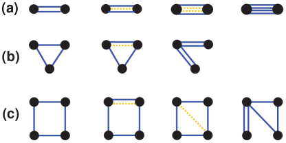
Figure 20: Diagrammatic representation of the lowest order processes contributing to cluster-correlation terms (for a pure initial state of the bath) of and (a) $\delta\tilde{L}_{J}(i,j)$, (b) $\delta\tilde{L}_{J}(i,j,k)$, and (c) $\delta\tilde{L}_{J}(i,j,k,l)$. Solid (Dashed) line for off-diagonal (diagonal) spin-spin interaction.

Conditions (i) and (ii) ensure that $\ln\delta\tilde{L}_{J}(\mathcal{C})$ is at least $|\mathcal{C}|$th order in $(\lambda_{\mathrm{ff}}t_{\mathrm{d}})$, where $\lambda_{\mathrm{ff}}$ is the typical off-diagonal bath interactions. Taking the Taylor expansion of $\ln\delta\tilde{L}_{J}(i,j)$ as an example, the first few terms in the expansion are shown diagrammatically in Fig. 20(a), including the lowest, second-order term $(\lambda_{ij}^{\mathrm{ff}}t_{\mathrm{d}})^{2}$ (first diagram), the third-order term $(\lambda_{ij}^{\mathrm{d}}t_{\mathrm{d}})(\lambda_{ij}^{\mathrm{ff}}t_{\mathrm{d}})^{2}$ (second diagram), and the fourth-order terms $(\lambda_{ij}^{\mathrm{d}}t_{\mathrm{d}})^{2}(\lambda_{ij}^{\mathrm{ff}}t_{\mathrm{d}})^{2}$ (third diagram) and $(\lambda_{ij}^{\mathrm{ff}}t_{\mathrm{d}})^{4}$ (fourth diagram). Similarly, the Taylor expansion of $\ln\delta\tilde{L}_{J}(i,j,k)$ is shown diagrammatically in Fig. 20(b), including the lowest, third-order term $(\lambda_{ij}^{\mathrm{ff}}t_{\mathrm{d}})(\lambda_{jk}^{\mathrm{ff}}t_{\mathrm{d}})(\lambda_{ki}^{\mathrm{ff}}t_{\mathrm{d}})$ (first diagram), the fourth-order term $(\lambda_{ij}^{\mathrm{d}}t_{\mathrm{d}})(\lambda_{ij}^{\mathrm{ff}}t_{\mathrm{d}})(\lambda_{jk}^{\mathrm{ff}}t_{\mathrm{d}})(\lambda_{ki}^{\mathrm{ff}}t_{\mathrm{d}})$ and other terms obtained by interchanging$\ i,j,k$ (second diagram), the fourth-order term $(\lambda_{ij}^{\mathrm{ff}}t_{\mathrm{d}})^{2}(\lambda_{jk}^{\mathrm{ff}}t_{\mathrm{d}})^{2}$ and other terms obtained by interchanging$\ i,j,k$ (third diagram). The first few terms in the Taylor expansion of $\ln\delta\tilde{L}_{J}(i,j,k,l)$ are shown in Fig. 20(c), including the lowest, fourth-order term (first diagram) and a few fifth-order terms (other diagrams). For the Taylor expansion of $\ln\delta\tilde{L}_{J}(\mathcal{C})$ for a general cluster $\mathcal{C}$, the lowest-order term is the ring diagram formed by $|\mathcal{C}|$ off-diagonal interaction lines, such as the first diagram in Figs. 20(a)-20(c), thus $\ln\delta\tilde{L}_{J}(\mathcal{C})$ is $|\mathcal{C}|$th order in $\lambda_{\mathrm{ff}}t_{\mathrm{d}}$.

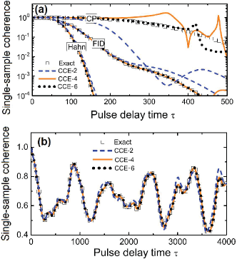
Figure 21: “True” decoherence from CCE compared with the exact solutions for one-dimensional spin-1/2 XY model consisting of $N=100$ bath spins. (a) FID, Hahn echo, and under CPMG-2 control. The level splitting of bath spins vary smoothly with location. (b) FID. The level splitting of bath spins varies randomly with location. Reproduced from Ref. Yang and Liu (2008b).

On a time scale $t_{\mathrm{d}}\ll$ $1/\lambda_{\mathrm{ff}}$, the exact CCE [Eq. (84)] can be truncated, e.g., the $M$th-order truncated CCE (CCE-$M$ for short) is:

$$\delta L_{J}^{(M)}=\prod_{|\mathcal{C}|\leq M}\delta\tilde{L}_{J}(\mathcal{C}).$$ (85)

For a relatively small truncation size $M,$ the cluster-correlation terms can be calculated by exact numerical diagonalization. CCE-1 gives $\delta L_{J}^{(1)}=\delta\tilde{L}_{J}(1)\cdots\delta\tilde{L}_{J}(N)$, corresponding to the independent precession of individual bath spin in the mean-field produced by other bath spins. CCE-2 accounts for the irreducible bath spin correlations up to pairs and is equivalent to the pair-correlation approximation Yao et al. (2006); Liu et al. (2007); Yao et al. (2007). Going to successively higher order truncations allows systematic inclusion of successively higher-order irreducible correlations in the spin bath evolution and accurate description of the decoherence under various DD controls [Fig. 21(a)].

In terms of $\tilde{\pi}(\mathcal{C})$ in Sec. VIII.4.1, we have $e^{\tilde{\pi}(\varnothing)}=L_{J}(\varnothing)$ and $e^{\tilde{\pi}(\mathcal{C})}=\delta\tilde{L}_{J}(\mathcal{C})$ for non-empty $\mathcal{C}$, thus a sufficient condition for convergence is still Eq. (72). However, in some cases, the convergence could even go well beyond. One such scenario is a disordered spin bath with highly non-uniform or even random spin splitting energies for different spins. In this case the disorder induced localization effect would bound the size of irreducible fully correlated clusters up to a critical size $M_{0}$, such that CCE-$M_{0}$ would converge to the exact results on any time scales [see Fig. 21(b) for an example].

The random spin splitting of bath spins inside a cluster $\mathcal{C}$ may come from their random couplings to the central spin or to the mean-field averages of other bath spins outside cluster $\mathcal{C}$, e.g., in $\delta\hat{H}_{\mathcal{C}}$, the spin splitting of the $j$th spin inside $\mathcal{C}$ consists of two non-uniform parts: $s(z)a_{j}/2$ due to HFI and $\sum_{k\notin\mathcal{C}}\lambda_{jk}^{\mathrm{d}}\langle J|\hat{I}_{k}^{z}|J\rangle$ due to coupling to external bath spins. This observation makes it possible to modify the CCE to improve its convergence Witzel et al. (2012a). The hybrid CCE Witzel et al. (2012a) is the same as the CCE in Sec. VIII.4.2 except for a different definitions of $\hat{H}_{\mathcal{C}}(z)$ and hence $L(\mathcal{C})$ [Eq. (73)]: instead of dropping all the bath spins outside cluster $\mathcal{C}$ from the bath Hamiltonian $\hat{H}(z)$, now $\hat{H}_{\mathcal{C}}(z)$ is obtained from $\hat{H}(z)$ by dropping the terms that flip the bath spins outside cluster $\mathcal{C}$. Thus $L(\mathcal{C})$ in hybrid CCE is connected to the cluster-correlation terms $\delta L_{J}(\mathcal{C})$ in Sec. VIII.4.3 via

$$L(\mathcal{C})=\sum_{J}P_{J}L_{J}(\varnothing)\delta L_{J}(\mathcal{C})=\sum_{J}P_{J}L_{J}(\mathcal{C}).$$ (86)

The mean fields from external bath spins randomizes the splitting of bath spins inside $\mathcal{C}$ and improves the convergence, although it is not obvious whether or not the hybrid CCE converges to the exact results: here $L(\mathcal{C})$ is no longer factorizable even if $\mathcal{C}$ can be divided into two subsets with no inter-subset interactions, so $\ln\tilde{L}(\mathcal{C})$ [as defined in Eq. (74)] does not vanish even if the interactions contained in $\hat{H}_{\mathcal{C}}(z)$ cannot connect all the spins in group $\mathcal{C}$ into a linked cluster. In practice, the ensemble average in Eq. (86) has exponential complexity. The algorithm to deal with this issue and detailed discussion of its applications to Si:P, silicon QDs, and NV centers can be found in Ref. Witzel et al. (2012a).

Finally, when the spin bath consists of many non-overlapping subsets $\mathcal{C}_{1},\mathcal{C}_{2},\cdots$ with weak inter-subset interactions, we can regard each subset as an effective bath spin and apply the CCE formalism [Eqs. (83) and (84)] to these effective spins, in the same way as Eqs. (78) and (79).

VIII.4.4 CCE for quantum noise auto-correlation function

Recently, the idea of CCE has been adapted Witzel et al. (2014); Ma et al. (2015) to calculate the auto-correlation $\langle\hat{b}(t)\hat{b}\rangle$ of the quantum noise $\hat{b}(t)\equiv e^{i\hat{H}_{B}t}\hat{b}e^{-i\hat{H}_{B}t}$ driven by an interacting bath Hamiltonian $\hat{H}_{B}$, where the noise operator $\hat{b}=\sum_{j}\hat{b}_{j}$ is the sum of operators of individual spins (e.g., $\hat{b}_{j}=\mathbf{a}_{j}\cdot\hat{\mathbf{I}}_{j}$) and $\langle\cdots\rangle\equiv\operatorname*{Tr}[\hat{\rho}_{B}(\cdots)]$ is the ensemble average in a product bath state $\hat{\rho}_{B}=\otimes_{j}\hat{\rho}_{j}$. The first step is to define the quantum noise from a spin cluster,

$$\hat{b}_{\mathcal{C}}(t)\equiv e^{i\hat{H}_{\mathcal{C}}t}\hat{b}_{\mathcal{C}}e^{-i\hat{H}_{\mathcal{C}}t}$$

where $\hat{b}_{\mathcal{C}}=\sum_{j\in\mathcal{C}}\hat{b}_{j}$ and $\hat{H}_{\mathcal{C}}$ is the Hamiltonian of a cluster $\mathcal{C}$, obtained from the bath Hamiltonian by dropping all bath spins except for those in cluster $\mathcal{C}$. The second step is to define the noise auto-correlation

$$C_{\{1,2,\cdots,N\}}(t)\equiv\langle\hat{b}(t)\hat{b}\rangle-\langle\hat{b}(t)\rangle\langle\hat{b}\rangle$$ (87)

and the contribution from a cluster $\mathcal{C}$:

$$C_{\mathcal{C}}(t)\equiv\langle\hat{b}_{\mathcal{C}}(t)\hat{b}_{\mathcal{C}}\rangle-\langle\hat{b}_{\mathcal{C}}(t)\rangle\langle\hat{b}_{\mathcal{C}}\rangle,$$ (88)

where $N$ is the number of bath spins. If a cluster $\mathcal{C}$ consists of two subsets $\mathcal{C}_{1}$ and $\mathcal{C}_{2}$ and $\hat{H}_{\mathcal{C}}$ does not contain any interaction between these two subsets, then the noise auto-correlation from this cluster is additive: $C_{\mathcal{C}}(t)=C_{\mathcal{C}_{1}}(t)+C_{\mathcal{C}_{2}}(t)$. This motivates the definition of a hierarchy of cluster-correlation terms:

$$\tilde{C}_{\mathcal{C}}(t)\equiv C_{\mathcal{C}}(t)-\sum_{\mathcal{C}^{\prime}\subset\mathcal{C}}\tilde{C}_{\mathcal{C}^{\prime}}(t),$$ (89)

e.g., $\tilde{C}_{i}(t)\equiv C_{i}(t)$, $\tilde{C}_{\{i,j\}}(t)\equiv C_{\{i,j\}}(t)-\tilde{C}_{i}(t)-\tilde{C}_{j}(t)$, etc. By definition, the pair-correlation $\tilde{C}_{\{i,j\}}(t)$ vanishes when there is no interaction between spin $i$ and spin $j$, thus $\tilde{C}_{\{i,j\}}(t)$ is at least first order in the bath spin interactions. Similarly, $\tilde{C}_{\mathcal{C}}(t)$ vanishes when the interactions contained in $\hat{H}_{\mathcal{C}}$ cannot connect the spins in group $\mathcal{C}$ into a linked cluster, thus $\tilde{C}_{\mathcal{C}}(t)$ is at least $(|\mathcal{C}|-1)$th order in the bath spin interactions. Finally, the noise auto-correlation is approximated by truncating the expansion, e.g., keeping cluster-correlation terms containing up to $M$ spins gives (CCE-$M$ for short):

$$C_{\{1,2,\cdots,N\}}^{(M)}(t)=\sum_{\mathcal{C},|\mathcal{C}|\leq M}\tilde{C}_{\mathcal{C}}(t).$$ (90)

Since $C_{\mathcal{C}}(t)$ and hence $\tilde{C}_{\mathcal{C}}(t)$ for small $|\mathcal{C}|$ can be easily calculated by exact numerical diagonalization, Eq. (90) provides a systematic approach to calculate the auto-correlation up to successively higher orders of inter-spin correlation, e.g., for a non-interacting spin bath, the cluster contributions $\tilde{C}_{\mathcal{C}}(t)=0$ for $|\mathcal{C}|\geq 2$, so CCE-1 gives the exact result: $C(1,2,\cdots,N)=\sum_{i}\tilde{C}(i)=\sum_{i}C(i)$, even in the presence of rapid single-spin dynamics such as that induced by the anisotropic HFI (see Sec. IX.1.2).

We notice that the original formulation Witzel et al. (2014); Ma et al. (2015) of the CCE of noise auto-correlation uses a slightly different definition:

$$C_{\{1,2,\cdots,N\}}^{\prime}(t) \equiv\langle\hat{b}(t)\hat{b}\rangle-\langle\hat{b}^{2}\rangle,$$ (91)

$$C_{\mathcal{C}}^{\prime}(t) \equiv\langle\hat{b}_{\mathcal{C}}(t)\hat{b}_{\mathcal{C}}\rangle-\langle\hat{b}_{\mathcal{C}}^{2}\rangle$$ (92)

instead of Eqs. (87) and (88). In this case, even when a cluster $\mathcal{C}$ consists of two subsets $\mathcal{C}_{1}$ and $\mathcal{C}_{2}$ and $\hat{H}_{\mathcal{C}}$ does not contain any interaction between these two subsets, the cluster term $C_{\mathcal{C}}^{\prime}(t)$ does not reduce to $C_{\mathcal{C}_{1}}^{\prime}(t)+C_{\mathcal{C}_{2}}^{\prime}(t)$ due to the existence of cross-correlation terms $(\langle\hat{b}_{\mathcal{C}_{1}}(t)\rangle-\langle\hat{b}_{\mathcal{C}_{1}}\rangle)\langle\hat{b}_{\mathcal{C}_{2}}\rangle$ and $(\langle\hat{b}_{\mathcal{C}_{2}}(t)\rangle-\langle\hat{b}_{\mathcal{C}_{2}}\rangle)\langle\hat{b}_{\mathcal{C}_{1}}\rangle$. Thus this formulation is essentially a short-time perturbative expansion of $W(t)$ around $t=0$ Witzel et al. (2014). For a maximally mixed bath state $\hat{\rho}_{B}\propto\hat{I}$, the cross-correlation terms vanish, thus $C_{\mathcal{C}}^{\prime}(t)=C_{\mathcal{C}}(t)-C_{\mathcal{C}}(0)$, i.e., the original formulation coincides with Eqs. (87)-(89).

VIII.4.5 Numerical techniques

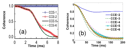
Figure 22: Convergence of CCE in realistic nuclear spin baths. (a) Decoherence of the NV electron spin transition $|+1\rangle\leftrightarrow|-1\rangle$ under CPMG-5 control and $B=0.3$ T along the NV axis, caused by the ¹³C nuclear spins with natural abundance 1.1%. (b) Decay of Hahn echo of the Bi donor electron spin near the “clock” transition ($B=B_{\mathrm{CT}}+0.3$ mT with $B_{\mathrm{CT}}=79.9$ mT), caused by the ²⁹Si nuclear spins with natural abundance 4.7%. Panal (a) is extracted from Ref. Zhao et al. (2011b) and panal (b) is extracted from the Supplementary Information of Ref. Ma et al. (2015).

The CCE calculations converge rapidly for the electron spin decoherence in nuclear spin baths with short-ranged dipolar interactions, such as the decoherence of the electron spin of an NV center caused by the ¹³C nuclear spins with natural abundance 1.1% in diamond Zhao et al. (2011b, a, 2012b) and the decoherence of the donor (phosphorus or bismuth) electron spin caused by the ²⁹Si nuclear spins with natural abundance 4.7% in silicon Witzel and Das Sarma (2007a); George et al. (2010); Ma et al. (2014); Balian et al. (2014); Ma et al. (2015); Balian et al. (2015), as shown in Fig. 22. Here we summarize the main steps of performing the CCE calculations in realistic systems and provide the numerical tricks in each step Witzel et al. (2012a); Zhao et al. (2012b); Ma et al. (2014, 2015).

Step 1: choosing the initial state of the bath. Since the maximally mixed thermal bath state and a typical pure product bath state sampled from the thermal ensemble give similar “true” decoherence (see Sec. V.2), especially for a relatively large bath (such as the ²⁹Si nuclear spin bath in silicon), it is preferrable to calculate the “true” decoherence with the CCE method for a pure bath state (Sec. VIII.4.3), which has faster convergence Witzel et al. (2012a); Ma et al. (2015) than that for a general noninteracting bath state (VIII.4.2). The thermal noise is relevant only for the FID and amounts to a multiplicative factor $L_{\mathrm{inh}}(t)$ [Eq. (59)].

Step 2: determining the size of the nuclear spin bath. The bath spins can be chosen as those within a certain threshold distance $R_{\mathrm{c}}$ away from the central spin (or threshold HFI strength), which is gradually increased till convergence. Typically $R_{\mathrm{c}}\sim 4$ nm (including $N\sim 500$ bath spins) for the natural ¹³C nuclear spin bath in diamond Zhao et al. (2011b, a) and $R_{\mathrm{c}}\sim 8$ nm (including $N\sim 5000$ bath spins) for the natural ²⁹Si nuclear spin bath in silicon Ma et al. (2014, 2015).

Step 3: defining effective bath spins. A cluster of bath spins that are fully linked via very strong interactions is identified as a large effective spin, so the bath is divided into many non-overlapping, strongly linked clusters $\mathcal{C}_{1},\mathcal{C}_{2},\cdots$, or equivalently many effective spins. Then subsequent steps and the CCE all apply to these effective spins [cf. Eqs. (78) and (79)].

Step 4: selecting contributing clusters. For a given truncation size $M$, it is not necessary to keep all the clusters containing $M$ effective spins, since only clusters with fully correlated fluctuations contribute to central spin decoherence. For nuclear spins coupled through short-range dipolar interactions and within the central spin decoherence time, significant inter-spin correlation develops only among a few nearest neighbours, especially among those that are fully linked through sufficiently strong interactions. Thus it suffices to keep clusters whose diameter is smaller than a certain upper cutoff $d_{\mathrm{c}}$, which is gradually increased till convergence. Typically $d_{\mathrm{c}}\sim$ 1 nm for both the natural ¹³C nuclear spin bath in diamond and the natural ²⁹Si nuclear spin bath in silicon Zhao et al. (2011a); Ma et al. (2014, 2015). A lower cutoff $\lambda_{\min}$ in the cluster connectivity strength $\lambda_{\mathcal{C}}$ (defined as the smallest interaction necessary to complete the full connectivity of the cluster $\mathcal{C}$) is also preferred Witzel et al. (2012a).

Finally, Monte Carlo sampling technique can be used when there are too many contributing clusters.

VIII.5 Real-space cluster expansion

As one of the first quantum many-body theories for central spin decoherence, the density matrix cluster expansion Witzel et al. (2005); Witzel and Das Sarma (2006) provides a convenient method to include multi-spin correlations, in the spirit of the virial expansion for interacting gases in grand canonical ensembles. In terms of $L(\mathcal{C})$ defined in Eq. (73) of Sec. VIII.4.2, cluster expansion defines the (irreducible) cluster-correlation terms $\{W(\mathcal{C})\}$ by substracting all reducible parts:

$$W(i) \equiv L(i),$$ (93a)

$$W(i,j) \equiv L(i,j)-W(i)W(j),$$ (93b)

$$W(i,j,k) \equiv L(i,j,k)-W(i)W(j)W(k)-W(i)W(j,k)$$ (93c)

$$\quad-W(j)W(i,k)-W(k)W(i,j),$$ (93d)

$$\cdots$$

$$W(\mathcal{C}) \equiv L(\mathcal{C})-\sum_{\{\mathcal{C}_{\alpha}\}}\prod_{\mathcal{C}_{\alpha}}W(\mathcal{C}_{\alpha}),$$ (93e)

where in the last line the sum runs over all possible partitions of the cluster $$\mathcal{C} \mathcal{C}_{1},\mathcal{C}_{2},\cdots$$ into non-overlapping and non-empty subsets . The central spin coherence can be expressed exactly in terms of these cluster-correlation terms:

$$L=W(1,2,\cdots,N)+\sum_{\{\mathcal{C}_{\alpha}\}}\prod_{\mathcal{C}_{\alpha}}W(\mathcal{C}_{\alpha}),$$ (94)

where the sum in the last line runs over all possible partitions of all bath spins $\{1,2,\cdots,N\}$ into non-overlapping and non-empty subsets $\mathcal{C}_{1},\mathcal{C}_{2},\cdots$.

The cluster-correlation terms $\{W(\mathcal{C})\}$ in cluster expansion has very similar properties as the cluster-correlation terms $\tilde{L}(\mathcal{C})$ in CCE (see Sec. VIII.4.2), e.g., $W(\mathcal{C})$ vanishes if the interactions contained in $\hat{H}_{\mathcal{C}}(z)$ cannot connect all the spins in group $\mathcal{C}$ into a linked cluster, so $W(\mathcal{C})$ is at least $(|\mathcal{C}|-1)$th order in $(\lambda t_{\mathrm{d}})$, where $\lambda$ is the typical interaction strength in the bath. Keeping cluster-correlation terms containing up to $M$ spins gives the $M$th-order truncated cluster expansion (CE-$M$ for short):

$$L^{(M)}=\sum_{\{\mathcal{C}_{\alpha}\},|\mathcal{C}_{\alpha}|\leq M}\prod_{\mathcal{C}_{\alpha}}W(\mathcal{C}_{\alpha}),$$ (95)

where the sum runs over all possible partitions of the bath into non-overlapping non-empty clusters $\mathcal{C}_{1},\mathcal{C}_{2},\cdots$ of size up to $M$. In the cluster expansion for interacting gases in grand canonical ensembles with translational symmetry, the evaluation of a truncated cluster expansion reduces to the calculation of a finite number of cluster terms $\{W(\mathcal{C}_{\alpha})\}$ with $|\mathcal{C}_{\alpha}|\leq M$, which can be easily done by exact numerical diagonalization. For a finite-size spin bath or for a bath without translational symmetry, however, it is very difficult to calculate the sum in Eq. (95) even for a small $M$.

When all the cluster terms $\{W(\mathcal{C})\}$ are individually small, Eq. (95) can be approximated by a factorized form by adding some overlapping terms that are higher-order small quantities. For example, the contour Hamiltonian in Eq. (58) gives $W(i)=L(i)=1$ at the echo time of DD control, so CE-$M$ can be approximated by

$$\bar{L}^{(M)}=\prod_{1<|\mathcal{C}_{\alpha}|\leq M}[1+W(\mathcal{C}_{\alpha})]\approx\prod_{1<|\mathcal{C}_{\alpha}|\leq M}e^{W(\mathcal{C}_{\alpha})}.$$ (96)

Comparing the factorized form in Eq. (96) to the exact CE-$M$ in Eq. (95), the error $L_{\mathrm{err}}^{(M)}\equiv\bar{L}^{(M)}-L^{(M)}$

$$L_{\mathrm{err}}^{(M)} \equiv\bar{L}^{(M)}-L^{(M)}$$

$$=\sum_{i<j<k}W(i,j)W(j,k)+\sum_{i<j<k<l}W(i,j,k)W(k,l)+\cdots,$$ (97)

contains the products of all possible cluster terms sharing at least one spin. Such overlapping terms are higher-order small quantities and hence Eq. (96) is justified when each individual cluster term for $|\mathcal{C}_{\alpha}|>1$ is small, e.g., for large spin baths, where the number of contributing clusters is large and hence the contribution from each individual cluster remains small within the time scale of decoherence.

The error $L_{\mathrm{err}}^{(M)}$ from the overlapping terms becomes relevant for small spin baths, where the coherent dynamics of a small number of multi-spin clusters dominating the decoherence may persist well beyond the bath spin flip-flop time, such that the small-term condition is no longer satisfied. In this case the cluster expansion may not converge to the exact results.

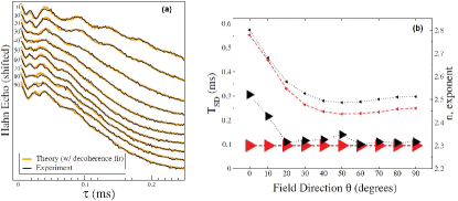
Figure 23: Spin echo decay in Si:P for ten different magnetic field orientations ranging from [001] to [110]. Apart from a few common fitting parameters for all curves, each curve are fitted with two parameters: the decoherence time $T_{\mathrm{SD}}$ due to ²⁹Si nuclei and its exponent $n$. These fitting parameters (black triangles) are compared with the cluster expansion calculations (red triangles) in (b). Right (Left) triangles correspond to $n$ ($T_{\mathrm{SD}}$). The fitted $n$ deviates from theory only at small magnetic field angles, where the nearest-neighbor dipolar flip-flop interactions approach zero. Reproduced from Ref. Witzel et al. (2007).

The factorized CE-$M$ [Eq. (96)] has been applied to electron and/or nuclear spin decoherence in Si:P (caused by ²⁹Si nuclei with natural abundance $4.7\%$) Witzel et al. (2005); Witzel and Das Sarma (2006, 2007b); Witzel et al. (2007), Si:Bi George et al. (2010), GaAs QDs (caused by ⁶⁹Ga, ⁷¹Ga, and ⁷⁵As nuclei), and Si:SiGe QDs (caused by ⁷³Ge and ²⁹Si nuclei) Witzel and Das Sarma (2006); Witzel et al. (2012b). For electron spin echo in Si:P, cluster expansion provides a complete understanding of the experimentally measured decay profile Tyryshkin et al. (2003); Abe et al. (2004); Ferretti et al. (2005); Tyryshkin et al. (2006); Abe et al. (2010) (see Fig. 23 for an example), including the envelope modulation by strong anisotropic HFI with a few proximal ²⁹Si nuclei (as discussed in Sec. IX.1.2), the dependence on the magnetic field orientations and ²⁹Si abundance, and the transition of the electron spin resonance lineshape from Gaussian (for ²⁹Si abundance $f\geq f_{0}$) to Lorentzian (for $f\leq 1.2\%$), which arises from ensemble averaging of the inhomogeneous dephasing $e^{-(t/T_{2}^{\ast})^{2}}$ of each individual donors over the distribution of $T_{2}^{\ast}$ Abragam (1961); Dobrovitski et al. (2008). Cluster expansion also shows that many-pulse CPMG could prolong the electron spin coherence time in Si:P and GaAs QDs by factors of 4–10 Witzel and Das Sarma (2007a) and that in Si:Bi system, the hybridization of the Bi donor electron spin with ²⁰⁹Bi nuclear spin could significantly changes the decay of the electron spin Hahn echo caused by the ²⁹Si nuclei George et al. (2010). For ³¹P donor nuclear spins in GaAs and Si Witzel and Das Sarma (2007b), cluster expansion gives negligible decoherence on the time scale of 100 $\mathrm{\mu s}$ in GaAs:P and 1-2 ms in Si:P under CPMG sequences with 2-4 $\pi$-pulses, indicating the promising role of ³¹P nuclear spin as a long-lived quantum memory.

VIII.6 Limitations of the many-body theories and possible extension

Despite the unprecedented understanding of the central spin decoherence under many experimental conditions, the available many-body theories are still subjected to several limitations. First, the theories in Sec. VIII are restricted to the pure dephasing model [Eq. (32) or (43)], which is justified when the central spin splitting $\gg$ bath spin splitting. A possible extension is to generalize the idea of CCE to spin relaxation, e.g., the evolution of $\langle\hat{S}_{z}(t)\rangle$ can be calculated by applying the CCE formalism to $L(t)\equiv\langle\hat{S}_{z}(t)\rangle/\langle\hat{S}_{z}(0)\rangle$. Second, for fast convergence of these theories, the size of the contributing bath spin clusters (i.e., those with appreciable correlated fluctuations) should be relatively small within the central spin decoherence time, so that their contributions can be obtained by exact diagonalization or other methods. Therefore, these theories also require short-range interactions between bath spins [i.e., small $q$ in Eq. (77) or Eq. (72)], which in turn necessitates a large central spin splitting. Otherwise (e.g., in weak magnetic fields Coish and Loss (2004); Coish et al. (2008); Cywiński et al. (2009b); Coish et al. (2010) or near the optimal work points Ma et al. (2015); Balian et al. (2015)) the successive flip-flops of the central spin with different bath spins may rapidly induce long-range correlations in the bath, beyond the description of existing theories.

For very small central spin spliting, the intrinsic bath spin interactions can be neglected, so the coupled system is described by the central spin model

$$\hat{H}=\omega_{0}\hat{S}_{z}+\omega_{I}\sum_{i}\hat{I}_{i}^{z}+\hat{\mathbf{S}}\cdot\hat{\mathbf{h}},$$ (98)

where $\hat{\mathbf{h}}\equiv\sum_{i}a_{i}\hat{\mathbf{I}}_{i}$. This model allows the central spin and the bath spins to exchange spin angular momentum, a feature that is absent from pure dephasing models. The central spin evolution due to Eq. (98) has been studied by a great diversity of approaches, including semi-classical models that treat the bath spins as classical stochastic variables Merkulov et al. (2002); Semenov and Kim (2003); Erlingsson and Nazarov (2004); Al-Hassanieh et al. (2006), exact analytical solutions for uniform HFI Melikidze et al. (2004); Kozlov (2007); Bortz and Stolze (2007) or fully polarized spin baths Khaetskii et al. (2002, 2003), and direct numerical modelling Schliemann et al. (2003); Cywinski et al. (2010); Dobrovitski and De Raedt (2003); Dobrovitski et al. (2003); Zhang et al. (2006) and Bethe ansatz solutions Faribault and Schuricht (2013a, b) for small baths containing a few tens of spins. For large baths, non-Markovian master equations Coish and Loss (2004); Coish et al. (2008, 2010); Breuer et al. (2004); Fischer and Breuer (2007); Ferraro et al. (2008) and equation of motion approaches Deng and Hu (2006, 2008) have been used, but they require strong magnetic fields under which central spin relaxation is suppressed while pure dephasing is usually dominated by the intrinsic nuclear spin interactions.

Recently, central spin decoherence on a time scale $\ll$ inverse of the HFI has been treated by the time-dependent density matrix renormalization group Stanek et al. (2013, 2014) and resumming the time-convolutionless master equation Barnes et al. (2012). The former shows that for large baths, the central spin dynamics is well described by the semi-classical model (Eq. (10)) with a classical Gaussian noise $\mathbf{\tilde{b}}(t)$, or by treating both the central spin and the bath spins as classical vectors subjected random initial orientations. The latter shows that the central spin dynamics depend on the HFI coefficients $\{a_{i}\}$ only through $\sum_{i}a_{i}^{2}$ and hence can be approximated by a exactly solvable model with uniform HFI, consistent with the energy-time uncertainty relations Barnes et al. (2011). The central spin dynamics on longer time scales, which depend sensitively on the specific distribution of $\{a_{i}\}$, remains an open issue.

IX Quantum decoherence effects

According to the idea of CCE, the contribution of bath dynamics to the central spin decoherence is the product of irreducible, correlated fluctuations from bath spin clusters of different sizes [see Eqs. (76) and (85)]. In this section we discuss some quantum decoherence effects caused by these fluctuations. In a relatively weak magnetic field or for the FID, the decoherence is dominated by the fluctuation of single-spin clusters, thus CCE-1 gives a good approximation Zhao et al. (2012b); Liu et al. (2012). In a strong magnetic field or under Hahn echo control, the fluctuation of single-spin clusters is frozen or its effect is suppressed by DD, and the correlated fluctuation of nuclear spin pairs dominates, thus CCE-2 is usually sufficient Zhao et al. (2012b, 2011b); Balian et al. (2014). Under high-order DD Zhao et al. (2012b); Ma et al. (2014) or near the optimal working points (e.g. for the electronic-nuclear hybrid spin qubit in Si:Bi system) Ma et al. (2015); Balian et al. (2015), multi-spin correlation becomes pronounced, so higher-order truncation of CCE are needed to get convergent results.

IX.1 Single spin fluctuation

In a relatively weak magnetic field, each individual nuclear spin has a large quantum fluctuation since the Zeeman energy and the HFI are comparable and do not commute with each other, while the pairwise nuclear flip-flop processes have much weaker effect as the dipolar interaction between nuclear spins is usually much weaker than the energy cost of the pairwise flip-flop due to HFI gradient. In this case, we can assume the central spin $\hat{\mathbf{S}}$ ($S=1/2$) is coupled to a bath of non-interacting nuclear spins $\{\hat{\mathbf{I}}_{j}\}$ ($I$=1/2 for simplicity), described by the pure dephasing Hamiltonian,

$$\hat{H}=\hat{S}_{z}\sum_{j}\mathbf{h}_{j}^{b}\cdot\hat{\mathbf{I}}_{j}+\sum_{j}\mathbf{h}_{j}^{B}\cdot\hat{\mathbf{I}}_{j},$$ (99)

where $\hat{b}\equiv\sum_{j}\mathbf{h}_{j}^{b}\cdot\hat{\mathbf{I}}_{j}$ with $\mathbf{h}_{j}^{b}$ being the HFI coupling, and the intrinsic bath Hamiltonian $\hat{H}_{B}=\sum_{j}\mathbf{h}_{j}^{B}\cdot\hat{\mathbf{I}}_{j}$ with $\mathbf{h}_{j}^{B}$ being the external magnetic field. The bath Hamiltonian conditioned on the central spin state is $\hat{H}_{\pm}=\sum_{j}\mathbf{h}_{j}^{(\pm)}\cdot\hat{\mathbf{I}}$ describing the bath spin precession around the fields $\mathbf{h}_{j}^{(\pm)}=\mathbf{h}_{j}^{B}\pm\mathbf{h}_{j}^{b}/2$.

The single-spin fluctuation causes two possible effects. For isotropic HFI, we have $[\hat{b},\hat{H}_{B}]=0$, so the thermal noise from bath spins leads to inhomogeneous dephasing of the central spin in FID. For anisotropic HFI [Eq. (50)], we have $[\hat{b},\hat{H}_{B}]\neq 0$, so the quantum noise from bath spins gives rise to modulation effects in central spin decoherence (see Appendix A for the Bloch vector representation of single nuclear spin dynamics).

IX.1.1 Isotropic HFI: inhomogeneous dephasing

For isotropic HFI (e.g., for conduction electron confined in a III-V semiconductor QD) Yao et al. (2006); Liu et al. (2007), $\mathbf{h}_{j}^{b}$ and $\mathbf{h}_{j}^{B}$ are both along the $z$ axis and Eq. (99) reduces to $\hat{H}=\hat{S}_{z}\sum_{j}{h}_{j}^{b}\hat{{I}}_{j}^{z}+\sum_{j}{h}_{j}^{B}\hat{{I}}_{j}^{z}$. In this case, $\hat{b}$ commutes with the bath Hamiltonian $\hat{H}_{B}$, so the noise is static and leads to Gaussian inhomogeneous dephasing for the FID (c.f. Eq. (59)),

$$L_{\mathrm{FID}}(t)=\prod_{j}\cos(h_{j}^{b}t/2)\approx e^{-(t/T_{2}^{\ast})^{2}},$$

where the inhomogeneous dephasing time $T_{2}^{\ast}=\sqrt{2}/h_{\mathrm{rms}}$ with $h_{\mathrm{rms}}=(1/2)\sqrt{\sum_{j}{(h_{j}^{b})}^{2}}$ being the root-mean-square fluctuation of the noise field Liu et al. (2012). DD can largely remove the effect of single-spin clusters. So one would have to go to higher order correlations of the nuclear spins to correctly describe the “true” decoherence.

IX.1.2 Anisotropic HFI: decoherence envelope modulation

For anisotropic HFI [Eq. (50)], the noise field $\mathbf{h}_{j}^{b}$ deviates from the direction of $\mathbf{h}_{j}^{B}$ (pointed along $z$ axis), then even non-interacting bath spins could cause nontrivial electron spin decoherence. The anisotropic HFI can exist for donors (or QDs) in silicon and NV centers in diamond (see Sec. VII.1.2). The FID is entirely determined by the magnitudes $h_{j}^{(\pm)}$ of the fields $\mathbf{h}_{j}^{(\pm)}$ and their relative angle $\Theta_{j}$:

$$L_{\mathrm{FID}}(t)=\prod_{j}L_{j}^{\mathrm{FID}}(t)$$

$$= \prod_{j}\left[\cos^{2}\frac{\Theta_{j}}{2}\cos\frac{(h_{j}^{(+)}-h_{j}^{(-)})t}{2}+\sin^{2}\frac{\Theta_{j}}{2}\cos\frac{(h_{j}^{(+)}+h_{j}^{(-)})t}{2}\right].$$ (100)

We decompose the anisotropic HFI as $\mathbf{h}_{j}^{b}=h_{j}^{b,z}\mathbf{e}_{z}+\mathbf{h}_{j}^{b,\perp}$. In the short-time limit, $L_{\mathrm{FID}}(t)$ shows Gaussian decay: $L_{\mathrm{FID}}(t)\approx e^{-\sum_{j}(h_{j}^{b,z})^{2}t^{2}/8}$ for $h_{j}^{b}\ll h_{j}^{B}$ and $L_{\mathrm{FID}}(t)\approx e^{-\sum_{j}(h_{j}^{b})^{2}t^{2}/8}$ for $h_{j}^{b}\gg h_{j}^{B}$ Zhao et al. (2012b). In a longer time-scale, since $\sin\Theta_{j}=(h_{j}^{b,\perp}h_{j}^{B})/(h_{j}^{(+)}h_{j}^{(-)})$, we have $|\sin\Theta|\ll 1$ for $h_{j}^{b}\gg h_{j}^{B}$ or $h_{j}^{b}\ll h_{j}^{B}$, thus in a strong external magnetic field ($h_{j}^{b}\ll h_{j}^{B}$), the $j$th nuclear spin contributes a dominant slow oscillation $\sim\cos(h_{j}^{b,z}t/2)$ modulated by a small-amplitude, fast oscillation $\sim\cos(h_{j}^{B}t)$ to the central spin decoherence Saikin and Fedichkin (2003). In QDs or shallow donors with a large nuclear spin bath, the rapid inhomogeneous dephasing usually makes this effect invisible. In diamond NV centers with a rather small nuclear spin bath, however, the electron spin decoherence is usually dominated by a few strongly coupled bath spins. In this case, the modulation effects is manifested as the deviation of the decoherence away from Gaussian profile, which has been observed experimentally Liu et al. (2012).

The Hahn echo

$$L_{\mathrm{H}}(2\tau)=\prod_{j}\left[1-2\sin^{2}\Theta_{j}\sin^{2}\frac{h_{j}^{(+)}\tau}{2}\sin^{2}\frac{h_{j}^{(-)}\tau}{2}\right]$$ (101)

shows non-Gaussian decay in the short time limit: $L_{\mathrm{H}}(2\tau)\approx e^{-|\mathbf{h}_{j}^{B}\times\mathbf{h}_{j}^{b}|^{2}\tau^{4}/8}$. On a longer time-scale, the second term in Eq. (101) gives rise to modulations with amplitude $\sim\sin^{2}\Theta_{j}$ on the electron spin echo decay (called electron spin echo envelope modulation, see Fig. 24 for an example), where $\sin\Theta_{j}$ is called the modulation depth parameter Witzel et al. (2007). The modulation depth is appreciable for those nuclei with the HFI and Zeeman energy comparable, i.e., $h_{j}^{b}\sim h_{j}^{B}$. When the magnetic field orientation (defined as the $z$ axis) is chosen such that $\mathbf{h}_{j}^{b}$ is perpendicular to $\mathbf{h}_{j}^{B}$ and hence $h_{j}^{(+)}=h_{j}^{(-)}=h_{j}$, periodic restoration of spin coherence can be achieved at $\sin(h_{j}\tau/2)=0$ Witzel et al. (2007).

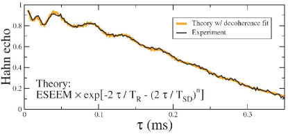
Figure 24: Theoretical and experimental results for electron spin echo decay. The theoretical curve is the product of spin echo envelope modulation due to anisotropic HFI induced bifurcated evolution of individual nuclear spins, the non-Markovian decay $e^{-(2\tau/T_{\mathrm{SD}})^{n}}$ due to nuclear spin flip-flop dynamics, and Markovian decay $e^{-2\tau/T_{2}}$. Reproduced from Ref. Witzel et al. (2007).

IX.2 Pair-correlation effect

In the strong magnetic field regime, the individual nuclear spin fluctuation are suppressed (apart from a trivial inhomogeneous dephasing for the FID), so central spin decoherence is caused by the correlated fluctuation of larger nuclear spin clusters. On a short time-scale compared with the inverse nuclear spin interactions, the correlated fluctuation is mainly from the nuclear spin pair dynamics, so it can be described by CCE-2 or equivalently the pair-correlation approximation Yao et al. (2006); Liu et al. (2007); Yao et al. (2007).

Here we focus on “true” decoherence and take the initial state of the nuclear spin bath as $|J\rangle$ [Eq. (56)]. For the Hamiltonian in Eq. (55), we have $\delta\tilde{L}_{J}(i)=1$ and hence

$$L_{J}=\prod_{\{i,j\}}L_{J}(i,j)$$

up to a trivial phase factor, where

$$L_{J}(i,j)\equiv\langle J|\mathcal{T}_{\mathrm{C}}e^{-i\int_{\mathrm{C}}\hat{H}(\hat{\mathbf{I}}_{i},\hat{\mathbf{I}}_{j},\{\langle J|\hat{\mathbf{I}}_{m\notin\{i,j\}}|J\rangle\})dz}|J\rangle$$

is the decoherence due to the nuclear spin pair $\{i,j\}$, whose effective Hamiltonian $\hat{H}(\hat{\mathbf{I}}_{i},\hat{\mathbf{I}}_{j},\{\langle J|\hat{\mathbf{I}}_{k\notin\{i,j\}}|J\rangle\})$ is obtained from the total Hamiltonian by replacing all spin operators outside cluster $\mathcal{C}$ by their mean-field averages.

There are $N(N-1)$ pairs in the bath, as labelled by $k\equiv(i,j)$. The initial state of the $k$th pair is mapped to the spin-down state of a spin-1/2 pseudospin $\hat{\boldsymbol{\sigma}}_{k}$: $|\Downarrow\rangle_{k}\equiv|m\rangle_{i}|n\rangle_{j}$, while the flip-flopped state is mapped to the spin-up state of this pseudo-spin: $|\Uparrow\rangle_{k}\equiv|m+1\rangle_{i}|n-1\rangle_{j}$. Therefore, the flip-flop dynamics of each nuclear spin pair are mapped to the flip dynamics of the pseudo-spins starting from the initial state $|J\rangle=\otimes_{k}|\Downarrow\rangle_{k}$. Here the flip of the $k$th pseudo-spin gives a state $|J,k\rangle$ that is energetically higher than $|J\rangle$ by an amount $\langle J,k|\hat{H}_{\pm}|J,k\rangle-\langle J|\hat{H}_{\pm}|J\rangle=D_{k}\pm Z_{k}$, while the transition amplitude from $|J\rangle$ to $|J,k\rangle$ is $\langle J,k|\hat{H}_{\pm}|J\rangle=B_{k}\pm A_{k}$, with $D_{k}$ from the diagonal nuclear spin interaction $\hat{H}_{\mathrm{d}}$, $B_{k}\propto\lambda_{ij}^{\mathrm{ff}}$ from the nuclear spin flip-flop interaction $\hat{H}_{\mathrm{ff}}$, $A_{k}\propto\tilde{\lambda}_{ij}^{\mathrm{ff}}$ from the electron spin mediated nuclear spin interaction $\tilde{H}_{\mathrm{ff}}$, and $Z_{k}=(a_{i}-a_{j})/2$ the energy cost of a pair flip due to the diagonal HFI $\hat{S}_{z}\hat{h}_{z}$. Thus $B_{k}$ and $D_{k}$ are nonzero only for neighboring nuclear spins (i.e., local pairs), while $A_{k}$ remains nonzero even for non-local pairs, but is suppressed under a strong magnetic field. The $k$th pseudospin is described by the Hamiltonian Yao et al. (2006); Liu et al. (2007); Yao et al. (2007)

$$\hat{H}_{k}^{\pm}=(2B_{k}\pm 2A_{k},0,D_{k}\pm Z_{k})\cdot\hat{\boldsymbol{\sigma}}_{k}/2\equiv\mathbf{h}_{k}^{(\pm)}\cdot\hat{\boldsymbol{\sigma}}_{k}/2.$$

Typically $|Z_{k}|\gg|B_{k}|\sim|D_{k}|\gg|A_{k}|$, thus the pseudo-spin dynamics is dominated by its coupling to the central spin. The pseudo-spin description provides a transparent geometric picture for central spin decoherence and its control by DD in terms of Bloch vectors, as well as magic coherence recovery via controlled disentanglement Liu et al. (2007); Yao et al. (2007).

IX.2.1 Non-local and local pair correlations

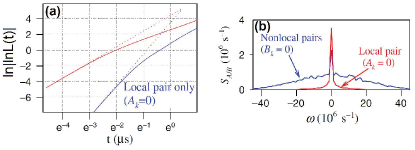
Figure 25: (a) Non-Markovian-to-Markovian crossover in electron spin decoherence. The dotted lines are the short-time profile. (b) Excitation spectra for nonlocal and local nuclear spin pairs. Reproduced from Ref. Liu et al. (2007).

The pseudo-spins are separated into two groups, corresponding to local pairs (group $\mathbb{G}_{B}$) with $\mathbf{h}_{k}^{(\pm)}\approx(2B_{k},0,\pm Z_{k})$ and nonlocal pairs (group $\mathbb{G}_{A}$) with $\mathbf{h}_{k}^{(\pm)}\approx\pm(2A_{k},0,Z_{k})$, respectively. Thus the central spin coherence is factorized as $\left|L_{J}(t)\right|=\left|L_{A}(t)\right|\times\left|L_{B}(t)\right|$, where $\left|L_{A/B}(t)\right|\equiv\prod_{k\in\mathbb{G}_{A/B}}|L_{k}(t)|$. These two kinds of nuclear spin pairs have qualitatively different contributions to electron spin decoherence, for both FID and under DD control.

Within the time scale of interest $t\ll 1/|B_{k}|,1/|A_{k}|$, the contributions from local and nonlocal pairs to the FID are Yao et al. (2006); Liu et al. (2007); Yao et al. (2007)

$$\left|L_{A}(t)\right| =\prod_{k\in\mathbb{G}_{A}}e^{-2t^{2}A_{k}^{2}\operatorname{sinc}^{2}(Z_{k}t)}=e^{-2t\int S_{A}(x/t)\operatorname{sinc}^{2}(x)dx},$$ (102)

$$\left|L_{B}(t)\right| =\prod_{k\in\mathbb{G}_{B}}e^{-(t^{4}/2)B_{k}^{2}Z_{k}^{2}\operatorname{sinc}^{4}\frac{Z_{k}t}{2}}=e^{-\frac{1}{2}t\int S_{B}(x/t)x^{2}\operatorname{sinc}^{4}\frac{x}{2}dx},$$ (103)

with

$$S_{A}(\omega) \equiv\sum_{k\in\mathbb{G}_{A}}\delta(\omega-Z_{k})A_{k}^{2},$$ (104)

$$S_{B}(\omega) \equiv\sum_{k\in\mathbb{G}_{B}}\delta(\omega-Z_{k})B_{k}^{2},$$ (105)

which are the pseudo-spin excitation spectra [see Fig. 25(b)]. In the short-time limit ($t\ll 1/|Z_{k}|$), the decoherence caused by non-local pairs is

$$\left|L_{k\in\mathbb{G}_{A}}(t)\right|\approx e^{-(t/T_{2,A})^{2}},$$ (106)

which shows Gaussian decay [red lines in Fig. 25(a)] on a time scale

$$T_{2,A}=\frac{1}{\sqrt{2\sum_{k\in\mathbb{G}_{A}}A_{k}^{2}}},$$ (107)

while the decoherence caused by local pairs is

$$\left|L_{k\in\mathbb{G}_{B}}(t)\right|\approx e^{-(t/T_{2,B})^{4}}$$ (108)

which shows quartic decay [blue lines in Fig. 25(a)] on a time scale

$$T_{2,B}=\frac{1}{(\sum_{k\in\mathbb{G}_{B}}B_{k}^{2}Z_{k}^{2}/2)^{1/4}}.$$ (109)

Here the Gaussian decay in Eq. (106) is actually the expansion of the power-law decay in Eq. (66) in the short-time limit $t\ll T_{\mathrm{dyn}}$, and $T_{2,A}$ is equivalent to $T_{\mathrm{dyn}}$, which is independent of the specific distribution of the HFI coefficients $\{a_{i}\}$ because the differences $a_{i}-a_{j}$ is unimportant due to energy-time uncertainty in the short-time regime Coish et al. (2010). On longer time scales, the sinc function dictates that only pairs with $\omega\in[-1/t,1/t]$ contribute significantly, indicative of energy conservation condition. For sufficiently large $t$ such that $S_{A/B}(\omega)$ can be regarded as constant $\bar{S}_{A/B}$ within $[-1/t,1/t]$, both $|L_{A}(t)|$ and $|L_{B}(t)|$ show exponential decay [see Fig. 25(a)] on time scales that depend sensitively on the distribution of the HFI coefficients (since energy conservation becomes important for long-time dynamics), in agreement with the ring diagram approximation [see the discussions after Eq. (67)]. The crossover from power-law decay to exponential decay indicates the crossover from the non-Markovian regime $(t\ll 1/Z_{k})$ to the Markovian regime $(t>1/Z_{k})$. Similar results have also been derived by a non-Markovian master equation approach Coish et al. (2010). For even longer times (which are relevant for a highly polarized spin bath), the decoherence is determined by the complex structure of the collective modes of the bath and becomes very sensitive to the distribution of $\{a_{i}\}$, e.g., exponential decay Cywiński et al. (2009b) and power-law decay Coish et al. (2010); Deng and Hu (2006, 2008) have been predicted.

Under DD control, the central spin decoherence caused by non-local nuclear spin pairs are largely suppressed, while the local pairs contributes most to central spin decoherence Yao et al. (2006); Liu et al. (2007). Under Hahn echo control, the central spin coherence at the echo time $t=2\tau$ is Yao et al. (2006); Liu et al. (2007); Yao et al. (2007)

$$L_{\mathrm{H}}(2\tau)\approx\prod_{k\in\mathbb{G}_{B}}e^{-2\tau^{4}Z_{k}^{2}B_{k}^{2}\operatorname{sinc}^{4}(Z_{k}\tau/2)}=e^{-2\tau\int S_{B}(x/\tau)x^{2}\operatorname{sinc}^{4}(x/2)dx},$$

which shows quartic decay $e^{-(2\tau/T_{\mathrm{H}})^{4}}$ with coherence time $T_{\mathrm{H}}=\sqrt{2}T_{2,B}$, which is $\sqrt{2}$ times that of the FID time. This shows that disturbing the central spin state changes the bifurcated bath evolution, which in turn changes the central spin decoherence. At the longer time-scale $1/|Z_{k}|\ll\tau\ll 1/|B_{k}|$, the coherence decays exponentially, indicative of Markovian behavior Yao et al. (2006); Liu et al. (2007).

IX.2.2 Magic coherence recovery

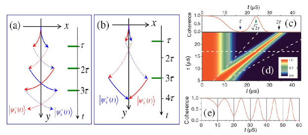
Figure 26: (a) Bifurcated trajectories of pseudo-spins Bloch vectors under the control of a sequence of equally spaced $\pi$-pulses. (b) similar to (a) but for the CPMG-2 control. (c) “True” decoherence under Hahn echo control, with the $\pi$-pulse applied at $\tau=17$ $\mathrm{\mu s}$ (indicated by the blue arrow). (d) Contour plot of “true” decoherence under Hahn echo vs. evolution time $t$ and pulse delay time $\tau$. The left tilted dashed line indicates $t=\tau$. The right tilted dashed line indicates the echo time $t=2\tau$. The horizontal line is the cut for the curve in (c). (e) “True” decoherence under a sequence of $\pi$-pulses (indicated by purple vertical lines) at intervals of 10 $\mathrm{\mu s}$. Panels (a) and (b) are extracted from Refs. Liu et al. (2007), and panels (c)-(e) are extracted from Ref. Yao et al. (2007).

The magic recovery of central spin coherence was predicted for an central electron spin in a nuclear spin bath in the strong field regime (HFI $\ll$ nuclear Zeeman splitting) Yao et al. (2007). In this case, the noise operator $\hat{b}=\sum_{j}a_{j}\hat{I}_{j}^{z}$ comes from the isotopic HFI between the electron spin and the nuclear spins. For nuclear spin-1/2’s, the flip-flop $|\uparrow\rangle_{i}|\downarrow\rangle_{j}\leftrightarrow|\downarrow\rangle_{i}|\uparrow\rangle_{j}$ of each nuclear spin pair $k\equiv(i,j)$ is mapped to the precession of the $k$th pseudo-spin $\boldsymbol{\sigma}_{k}$: $|\Uparrow\rangle_{k}\equiv|\uparrow\rangle_{i}|\downarrow\rangle_{j}$ and $|\Downarrow\rangle_{k}\equiv|\downarrow\rangle_{i}|\uparrow\rangle_{j}$. The pseudospin field is $\mathbf{h}_{k}^{(\pm)}=\mathbf{h}_{k}^{B}\pm\mathbf{h}_{k}^{b}/2$ with $\mathbf{h}_{k}^{B}=X_{k}^{B}\mathbf{e}_{x}+Z_{k}^{B}\mathbf{e}_{z}$ and $\mathbf{h}_{k}^{b}=Z_{k}^{b}\mathbf{e}_{z}$, where $X_{k}^{B},Z_{k}^{B}$ are the intrinsic nuclear spin flip-flop amplitude and energy cost, respectively, due to nuclear dipolar interactions, while $Z_{k}^{b}$ is the HFI induced correction to the energy cost.

The bifurcated evolution $|J\rangle\rightarrow|J_{\pm}(t)\rangle$ of the pseudospin starting from a pure state (say $|J\rangle=|\Uparrow\rangle$) can be mapped to Bloch vectors $\boldsymbol{\sigma}_{\pm}(t)$ and the central spin decoherence is determined by their distance $d(t)=|\boldsymbol{\sigma}_{+}(t)-\boldsymbol{\sigma}_{-}(t)|$ (see the Appendix). When $Z_{k}^{B}=0$, the fields $\mathbf{h}_{k}^{(\pm)}=(X_{k}^{B},0,\pm Z_{k}^{b})$ leads to $t^{2}$ increase of $d(t)$ in the short-time limit, while the application of a $\pi$ pulse at time $\tau$ reverse the evolution direction and gives rise to coherence recovery at the magic time $t_{\mathrm{mag}}=\sqrt{2}\tau$ instead of the echo time $t_{\mathrm{d}}=2\tau$ (see the Appendix). Here the presence of $Z_{k}^{B}$ does not change the $t^{2}$ increase of $d(t)$, so it shows the same magic coherence recovery [see Fig. 26(b) and (c)]. More generally, under an arbitrary DD characterized by the modulation function $s(t)$, the distance

$$d^{(1)}(t)\propto\int_{0}^{t}t^{\prime}s(t^{\prime})dt^{\prime}$$ (110)

vanishes (and hence coherence recovery occurs) at the magic time $t_{\mathrm{mag}}$ as determined by $\int_{0}^{t_{\mathrm{mag}}}ts(t)dt=0$, e.g., $t_{\mathrm{mag}}=\sqrt{N(N+1)}\tau$ for the DD consisting of $N$ equally spaced $\pi$-pulses $\tau_{k}=\tau$ [see Fig. 26(a) and (d)]. By contrast, in the absence of intrinsic bath dynamics ($\mathbf{h}_{k}^{B}=0$), the distance $d(t)\propto t$. Under DD control, the distance

$$d^{(0)}(t)\propto\int_{0}^{t}s(t^{\prime})dt^{\prime}$$ (111)

vanishes at the echo time $t_{\mathrm{d}}=2\tau$, corresponding to the elimination of inhomogenous dephasing at the echo time.

Equations (110) and (111) are reminiscent of the Taylor expansion of the classical random phase $\tilde{\varphi}(t_{\mathrm{d}})=\int_{0}^{t_{\mathrm{d}}}s(t)\tilde{b}(t)dt\approx\sum_{n}\tilde{b}_{n}\int_{0}^{t_{\mathrm{d}}}s(t)t^{n}dt$ based on $\tilde{b}(t)=\sum_{n}\tilde{b}_{n}t^{n}$. For a pure initial state of the bath (no classical analog), the lowest-order term $d^{(0)}(t)$ is absent, so $d^{(1)}(t)=0$ gives rise to magic coherence recovery at $t_{\mathrm{mag}}$, suggesting that elimination of the coupling to the environment is not an necessary condition for the recovery of coherence. For a thermal initial state of the bath, since the time-averaged coupling between the central spin and the bath is nonzero at the magic time in the first order, the rapid inhomogeneous dephasing will prevent magic coherence recovery from being observed. Direct observation of magic coherence recovery is possible once the inhomogeneous nuclear spin distribution is narrowed, e.g., a projective measurement of the noise operator $\hat{b}$ could be used to limit the nuclear spin configurations by post-selection Giedke et al. (2006); Klauser et al. (2006); Stepanenko et al. (2006).

IX.2.3 Anomalous decoherence effects

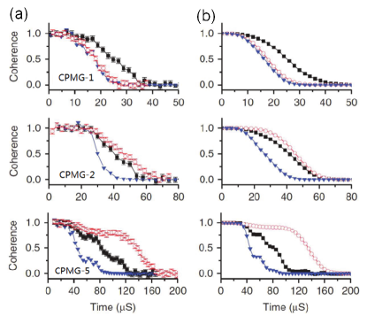
Figure 27: (a) Measured single (black line with square symbols) and double (red line with circle symbols) quantum coherence, under the control of different numbers of equally spaced pulses (CPMG-1, CPMG-2 and CPMG-5, from top to bottom). The scaled single quantum coherence $|L_{0,+1}|^{4}$ (blue line with triangle symbols) is also shown for comparison. (b) The theoretical results, plotted in the same format as in (a). Adapted from Ref. Huang et al. (2011).

An important feature of classical decoherence theories is that different processes coupled to the same noise source have similar decoherence behaviors and stronger noises cause faster decoherence. However, this is not the case in the quantum picture, since stronger coupling to the environment allows DD control to strongly manipulate the environmental dynamics to recover the lost coherence. For example, the spin-1 electronic state of the NV center in diamond with eigenstates $\{|m\rangle\}$ ($m=0,\pm 1$) is subjected to noises from the ¹³C nuclear spin bath. Surprisingly, under DD control, the double transition $|+1\rangle\leftrightarrow|-1\rangle$ could have longer coherence time than the single transition $|0\rangle\leftrightarrow|\pm 1\rangle$, even though the noise amplitude for the former is twice that for the latter Zhao et al. (2011b); Huang et al. (2011). This anomalous decoherence effect can be understood from the manipulation of pseudospin evolutions via DD control of the central spin.

In the semiclassical noise picture, the nuclear spin bath can be described as a random fluctuating local field Kubo (1954); Anderson (1954). For Gaussian noise Cywinski et al. (2008); Ma et al. (2015); Witzel et al. (2014), the central spin decoherence for the transition $|m\rangle\leftrightarrow|n\rangle$ is $L_{m,n}(t)=e^{-(m-n)^{2}\langle\tilde{\varphi}^{2}(t)\rangle/2}$, which obeys the scaling relation

$$|L_{+1,-1}(t)|=|L_{0,\pm 1}(t)|^{4},$$ (112)

We can see that decoherence of double transition $L_{+1,-1}(t)$ decays in the same way as that of single transitions $L_{0,\pm 1}(t)$, but is faster. The scaling relation in Eq. (112) remains valid when the electron spin is subjected to arbitrary DD control. However, numerical calculations in the quantum picture shows that under DD control with more and more $\pi$ pulses, the classical scaling relation in Eq. (112) is violated more and more significantly, and finally the double quantum coherence even decays slower than the single quantum coherence [see Fig. 27(b)].

This counterintuitive effect can be understood by analyzing the microscopic nuclear spin bath evolution $\hat{U}_{m}(t)\equiv e^{-i\hat{H}_{m}t}$ conditioned on the central spin state, where $\hat{H}_{m}\equiv\hat{H}_{B}+m\hat{b}$. Under a moderate magnetic field $(\gtrsim 0.1$ T) along the N-V symmetry axis ($z$ axis), the flip of individual nuclear spins is suppressed by the large nuclear Zeeman splitting, so the elementary excitation of the nuclear spins are the flip-flop of nuclear spin pairs, which can be mapped to the precession of non-interacting pseudo-spins with the effective Hamiltonian conditioned on the electron spin state,

$$\hat{H}_{m}^{\mathrm{eff}}=\sum_{k}\mathbf{h}_{k}^{(m)}\cdot\hat{\boldsymbol{\sigma}}_{k}=\sum_{k}(\mathbf{h}_{k}^{B}+m\mathbf{h}_{k}^{b})\cdot\hat{\boldsymbol{\sigma}}_{k}.$$

where $\mathbf{h}_{k}^{b}=Z_{k}\mathbf{e}_{z}$ comes from the HFI ($Z_{k}\equiv{{}_{k}}\langle\Uparrow|\hat{b}|\Uparrow\rangle_{k}-{{}_{k}}\langle\Downarrow|\hat{b}|\Downarrow\rangle_{k}$) and $\mathbf{h}_{k}^{B}=X_{k}\mathbf{e}_{x}$ is from the nuclear dipolar interaction ($X_{k}\equiv 2{{}_{k}}\langle\Uparrow|\hat{H}_{B}|\Downarrow\rangle_{k}$), so the coupling to the central spin dominates the bath dynamics ($h_{k}^{b}\gg h_{k}^{B}$). According to Eq. (101), the Hahn echo of electron spin coherence for the transition $|m\rangle\leftrightarrow|n\rangle$ is

$$L_{m,n}^{\mathrm{H}}(2\tau)=\prod_{k}\left[1-2\sin^{2}\Theta_{k}^{m,n}\sin^{2}\frac{h_{k}^{(m)}\tau}{2}\sin^{2}\frac{h_{k}^{(n)}\tau}{2}\right],$$

where $\Theta_{k}^{m,n}$ is the angle between $\mathbf{h}_{k}^{(m)}$ and $\mathbf{h}_{k}^{(n)}$. The decay in the short-time limit is

$$L_{m,n}^{\mathrm{H}}(2\tau)\approx\prod_{k}e^{-|\mathbf{h}_{k}^{(m)}\times\mathbf{h}_{k}^{(n)}|^{2}\tau^{4}/8}=\prod_{k}e^{-(m-n)^{2}|\mathbf{h}_{k}^{B}\times\mathbf{h}_{k}^{b}|^{2}\tau^{4}/8},$$

which obeys the classical scaling Eq. (112). At a longer time-scale, however, the strong coupling to the central spin makes the two fields of $L_{+1,-1}^{\mathrm{H}}(2\tau)$ nearly antiparallel $(\sin\Theta_{k}^{+1,-1}\ll 1)$, while that of the single quantum coherence are nearly perpendicular $(\sin\Theta_{k}^{0,\pm 1}\approx 1)$. Consequently, the long-time decay of the double quantum coherence is much smaller than that of the single quantum coherence, thus violating Eq. (112) at longer times. Application of more $\pi$ pulses prolongs the electron spin coherence time and makes this long-time behavior more pronounced.

This anomalous decoherence has been experimentally observed by Huang et al. in type-IIa diamond at room temperature Huang et al. (2011). In the experimental setup, the magnetic field is weak, so the electron spin decoherence is mainly caused by the single ¹³C nuclear spin dynamicis, quite similar to the pseudospin dynamics dicussed above.

IX.3 Multi-spin correlation effects

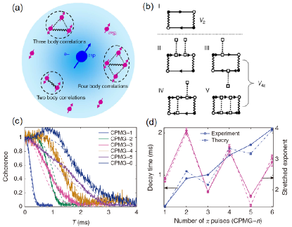
Figure 28: Revealing many-body correlations in nuclear spin baths by central spin decoherence. (a) Electron spin of a phosphorous donor in silicon interacts with a bath of ²⁹Si nuclear spin-1/2’s possessing various many-body processes. (b) topologically inequivalent connected Feynman diagrams corresponding to different many-body processes in the nuclear spin bath: (I) $V_{2}$ - second-order pairwise flip-flop, (II-V) $V_{4z}$ - fourth-order pairwise flip-flop dressed by diagonal interactions. (c) Measured (solid lines) and calculated (dashed lines) coherence of the P donor electron spin in the natural ²⁹Si nuclear spin bath under CPMG control. (d) Comparisons of the experimental (solid lines) and theoretical (dashed line) decay times $T_{\mathrm{SD}}$ (blue) and stretched exponents $n$ (magenta) of the central spin decoherence under the CPMG control in (c). Extracted from Ref. Ma et al. (2014).

The effects of multi-spin correlations on central spin decoherence become pronounced when the coherence time is prolonged to be comparable or longer than the inverse of typical nuclear-nuclear interaction, which can be realized by applying multi-pulse DD control Zhao et al. (2012b); Witzel and Das Sarma (2007a); Ma et al. (2014) or tuning the external magnetic field near some optimal working points Ma et al. (2015); Balian et al. (2014, 2015) (also called “clock” transitions Wolfowicz et al. (2013) where the central spin is insensitive to the magnetic noise in the first order). The CCE method can explicitly show the contributions of different multi-spin clusters in the nuclear spin bath to central spin decoherence, providing an intuitive tool to identify the underlying nuclear spin processes. For NV centers in diamond and donor spins in silicon, the CCE-2 calculations (truncated up to the clusters with two nuclear spins) always give converged results for Hahn echo of spin coherence Zhao et al. (2012b); Balian et al. (2014), indicating the pairwise flip-flop processes dominate the central spin decoherence. For central spin decoherence under multi-pulse DD control Zhao et al. (2012b) or near the optimal working points in silicon Ma et al. (2015); Balian et al. (2015) , the CCE-6 calculations (truncated up to the clusters with six nuclear spins) are always needed to give converged results, indicating that the multi-spin correlations contributes significantly to central spin decoherence.

More interestingly, recent studies show that DD control of the central spin can selectively suppress or amplify certain many-body processes in the nuclear spin bath Ma et al. (2014). In this case, LCE provides a systematic and transparent way to visualize the gradual development of different many-body processes in a nanoscale spin bath, by analysing the individual influence of each LCE diagram on the central spin decoherence Saikin et al. (2007). For example, consider a central electron spin in a relatively large nuclear spin bath with a strong external magnetic field and the HFI between the central spin and bath spins much larger than the nuclear-nuclear interactions, such as shallow donors in silicon (e.g. Si:P and Si:Bi) and electron spin in semiconductors (e.g. GaAs and InAs quantum dots). For CPMG-$N$ (or UDD-$N$) control of the central spin with odd $N$, the second-order pairwise flip-flop diagram ($V_{2}$ term in Fig. 28(b)) dominates the central spin decoherence and almost fully reproduces the exact decoherence calculated from CCE, while for CPMG-$N$ control with even $N$, the effects of the second-order pairwise flip-flop diagram are cancelled and the fourth-order flip-flop diagrams ($V_{4z}$ terms in Fig. 28(b)), corresponding to renormalized pairwise flip-flop dressed by the diagonal interactions (or pairwise flip-flop processes of two nuclear spins renormalized the dipolar diagonal interaction with the other nuclear spins in the bath), dominates the decoherence. This even-odd effect indicates that the second-order flip-flop [$V_{2}$ term Fig. 28(b)] and fourth-order flip-flop processes [$V_{4z}$ term in Fig. 28(b)] can be selectively detected by applying an appropriate number of DD pulses, as has been theoretically predicted and experimentally observed recently in Si:P system Ma et al. (2014). Actually, a similar even-odd effect has been noticed before in cluster expansion calculations Witzel and Das Sarma (2007a) (without analyzing the underlying microscopic processes): in the presence of an even (odd) number of DD pulses, the decoherence scale as $\ln L=O(\lambda^{4})$ [$\ln L=O(\lambda^{2})$] with respect to the dipolar interaction strength $\lambda$ between bath spins. In the experiment Ma et al. (2014), the measured decoherence $e^{-(t/T_{\mathrm{SD}})^{n}}$ caused by ²⁹Si nuclei has a stretching factor $n$ oscillating between about $2$ (for odd $N$) and $4$ (for even $N$), as shown in Figs. 28(c) and (d), indicating the detection of either the second-order flip-flop processes or fourth-order flip-flop processes. The different signatures of the many-body processes in the bath under DD control of the central spin, in particular the even-odd effect in the number of DD control pulses, provide a useful approach to studying many-body physics in the nuclear spin bath.

X Summary and outlook

Central electron spin decoherence in nanoscale nuclear spin baths is a critical issue for quantum technologies. In recent years, quantum pictures and quantum many-body theories have been established and have provided a quantitative description and unprecedented understanding for the central spin decoherence under many experimental conditions (such as DD control and moderate to strong magnetic fields). Accompanying the great progresses in prolonging the central spin coherence time through various DD schemes, the coherent evolution of the central spin in turn serves as an ultrasensitive probe for weak signals Chernobrod and Berman (2005); Degen (2008); Taylor et al. (2008); Hall et al. (2009, 2010) and many-body dynamics in the environments Quan et al. (2006); Chen et al. (2013); Wei and Liu (2012); Peng et al. (2015); Wei et al. (2014, 2015) with nanoscale resolution.

When the semi-classical noise model and especially the noise filter description are valid Ma et al. (2015), central spin decoherence under DD control has been used to reconstruct the environmental noise spectra Álvarez and Suter (2011); Bylander et al. (2011); Bar-Gill et al. (2012); Cywiński (2014), which in turn can be used to design optimal quantum control for protecting the quantum coherence and quantum gates Witzel et al. (2014). In particular, the decay of the central spin coherence on very long time scales (up to seconds Ma et al. (2015)) allows studying the low-energy excitations in the environment, since as the evolution time $t$ increases, the noises that cause significant central spin decoherence have frequencies $\sim 1/t$.

Central spin decoherence under DD control has also been widely used for quantum sensing of single nuclear spins Cole and Hollenberg (2009); Zhao et al. (2011a). When the period of the DD control matches the transition frequencies of the target nuclear spin(s) Zhao et al. (2011a), the noises from the target nuclear spins are resonantly amplified, causing enhanced central spin decoherence (manifested as a sharp coherence dip when sweeping the DD period). Several groups have adopted the DD scheme to successfully detect single ¹³C nuclear spins Zhao et al. (2012a); Kolkowitz et al. (2012); Taminiau et al. (2012) and ¹³C clusters Shi et al. (2014) in diamond. Shallow NV centers near the surface have also been used to sense the NMR of single protein molecules Shi et al. (2015) and nano-scale NMR of nuclear species Mamin et al. (2013); Staudacher et al. (2013) on diamond surfaces. Recently, there are also new proposals and concepts for quantum sensing, such as using multiple NV spins as the quantum sensor Ma et al. (2016), distinguishing nuclear spins of different species by sweeping the DD pulse number Ma and Liu (2016), and design of multi-dimensional DD to distinguish the nuclear spin correlations in single molecules Ma and Liu (2015); Boss et al. (2016).

Another promising direction is to employ the central spin decoherence to reveal the many-body physics and thermodynamic properties of the environment, since in some cases the central spin decoherence caused by the environment is directly related to the partition function of the environment. It has been found that central spin coherence shows sharp decay when the environment is tuned near a quantum critical point Quan et al. (2006); Chen et al. (2013). For a central spin homogenously coupled to a ferromagnetic Ising model, the central spin coherence vanishes at times corresponding to the Lee-Yang zeros of the partition function of the Ising model Wei and Liu (2012); Peng et al. (2015). Moreover, central spin decoherence has extended the phase transitions in the environment to the complex plane of physical parameters Wei et al. (2014) and enabled thermodynamic holograph of the partition function of the environment Wei et al. (2015).

XI Acknowledgements

We acknowledge the support by Hong Kong RGC, CUHK Vice Chancellor’s One-off Discretionary Fund, the NSFC (Grant No. 11274036 and No. 11322542), the MOST (Grant No. 2014CB848700), NSFC program for ’Scientific Research Center’ (Program No. U1530401), and the computational support from the Beijing Computational Science Research Center (CSRC).

Appendix A Bloch vector representation of single spin dynamics

Figure 29: Larmor precession of the Bloch vectors $\boldsymbol{\sigma}_{\pm}(t)$ of the two bath pathways around (a) $\mathbf{h}_{\pm}=(\pm X,0,Z)$ and (b) $\mathbf{h}_{\pm}=(X,0,\pm Z)$. (c) and (d) are the corresponding projection of the Bloch vectors in the $xoy$ plane.

We consider that the bath consists of a single spin-1/2, which starts from a pure spin-up state $|J\rangle=|\Uparrow\rangle$ along the $z$ axis and bifurcates into two pathways $|J_{\pm}(t)\rangle=e^{-i\hat{H}_{\pm}t}|J\rangle$ with

$$\hat{H}_{\pm}=\hat{H}_{B}\pm\hat{b}/2=(\mathbf{h}_{B}\pm\frac{\mathbf{h}_{b}}{2})\cdot\frac{\boldsymbol{\hat{\sigma}}}{2}.$$

The pathways can be mapped to the Bloch vectors $\boldsymbol{\sigma}_{\pm}(t)\equiv\langle J_{\pm}(t)|\hat{\boldsymbol{\sigma}}|J_{\pm}(t)\rangle$, which start from $\mathbf{e}_{z}$ at $t=0$ and then undergo Larmor precession around the fields $\mathbf{h}_{\pm}$ on a unit sphere. The central spin decoherence $|L(t)|^{2}=1-d^{2}(t)/4$ is determined by the distance $d(t)=|\boldsymbol{\sigma}_{+}(t)-\boldsymbol{\sigma}_{-}(t)|$ between the Bloch vectors Yao et al. (2006); Liu et al. (2007). To visualize the bifurcated bath evolution, we consider two special cases: (A) $\mathbf{h}_{\pm}=(\pm X,0,Z)$ and  (B) $\mathbf{h}_{\pm}=(X,0,\pm Z)$. In either case, the bath spin precesses with angular frequency $h=\sqrt{X^{2}+Z^{2}}$ on a circle of radius $\sin\theta=X/h$.

For case (A), the FID

$$L(t)=1-2\sin^{2}\theta\sin^{2}\frac{ht}{2}\overset{t\ll 1/h}{\longrightarrow}e^{-X^{2}t^{2}/2}$$

shows Gaussian decay in the short-time limit, corresponding to a linear increase of the distance $d(t)\approx 2Xt$ with time [Fig. 29(a) and (c)]. At $t=\pi/h$, the distance is maximal $d_{\max}=2\sin(2\theta)$ and the coherence is minimal: $L_{\min}=\cos(2\theta)$. Under Hahn echo control, the distance in the short-time limit is $d_{\mathrm{H}}(t)\approx 2X(\tau-(t-\tau))$, so central spin decoherence is minimized at the echo time

$$t_{\mathrm{d}}=2\tau.$$ (113)

For case (B), the FID Yao et al. (2006); Liu et al. (2007)

$$L(t) =1-2\cos^{2}\theta\sin^{2}\frac{ht}{2}-i\cos\theta\sin(ht)$$

$$\overset{t\ll 1/h}{\longrightarrow}e^{-iZt(1-X^{2}t^{2}/6)-Z^{2}X^{2}t^{4}/8}$$

exhibits $t^{4}$ decay in the short-time limit, corresponding to quadratic increase of the distance $d(t)\approx XZt^{2}$ with time [Fig. 29(b) and (d)]. At $t=\pi/h$, the distance is maximal $d_{\max}=2\sin(2\theta)$ and the coherence is minimal: $L_{\min}=\cos(2\theta)$. Under Hahn echo control, the distance in the short-time limit is $d_{\mathrm{H}}(t)\approx[(\tau^{2}-(t^{2}-\tau^{2})]XZ$, so central spin decoherence is minimized at the magic time:

$$t_{\mathrm{mag}}=\sqrt{2}\tau.$$ (114)

The different coherence recovery times [Eqs. (113) and (114)] follow from the different time dependences of the Bloch vector distances: $d(t)\propto t$ for case (A) and $d(t)\propto t^{2}$ for case (B). For case (A) [Fig. 29(c)], the Bloch vectors $\boldsymbol{\sigma}_{\pm}(t)$ move in opposite directions with almost constant velocity $X$. After the $\pi$ pulse, both Bloch vectors reverse their velocities, so minimal distance occurs at $2\tau$. For case (B) [Fig. 29(d)], both Bloch vectors move away from the $-y$ axis quadratically with time, e.g., the distance of each Bloch vector from the $-y$ axis reaches $\tau^{2}$ at $t=\tau$. If there were no $\pi$ pulses at $\tau$, then evolution from $\tau$ to $\sqrt{2}\tau$ would double the distance to $2\tau^{2}$. Now the $\pi$ pulse reverse the evolution direction of both Bloch vectors, so $\boldsymbol{\sigma}_{\pm}(t)$ both return to the $-y$ axis at $\sqrt{2}\tau$. Such coherence recovery at a “magic” time (i.e., different from the echo time) was first predicted in Ref. Yao et al. (2007); Liu et al. (2007) and will be discussed in more detail in Sec. IX.2.2.

References

- Benioff (1980) P. Benioff, Journal of Statistical Physics 22, 563 (1980).
- Feynman (1982) R. Feynman, Int. J. Theor. Phys. 21, 467 (1982).
- Deutsch (1985) D. Deutsch, Proceedings of the Royal Society of London A: Mathematical, Physical and Engineering Sciences 400, 97 (1985).
- Bennett and Brassard (1984) C. H. Bennett and G. Brassard, in Proceedings of the International Conference on Computers, Systems and Signal Processing, Vol. 175 (Bangalore, India, 1984) p. 8.
- Gisin et al. (2002) N. Gisin, G. Ribordy, W. Tittel, and H. Zbinden, Rev. Mod. Phys. 74, 145 (2002).
- Caves (1981) C. M. Caves, Phys. Rev. D 23, 1693 (1981).
- Budker and Romalis (2007) D. Budker and M. Romalis, Nat. Phys. 3, 227 (2007).
- Giovannetti et al. (2011) V. Giovannetti, S. Lloyd, and L. Maccone, Nat. Photon. 5, 222 (2011).
- DiVincenzo (1995) D. P. DiVincenzo, Science 270, 255 (1995).
- Ladd et al. (2010) T. D. Ladd, F. Jelezko, R. Laflamme, Y. Nakamura, C. Monroe, and J. L. O’Brien, Nature 464, 45 (2010).
- Leggett et al. (1987) A. J. Leggett, S. Chakravarty, A. T. Dorsey, M. P. A. Fisher, A. Garg, and W. Zwerger, Rev. Mod. Phys. 59, 1 (1987).
- Prokof’ev and Stamp (2000) N. V. Prokof’ev and P. C. E. Stamp, Rep. Prog. Phys. 63, 669 (2000).
- Zurek (2003) W. H. Zurek, Rev. Mod. Phys. 75, 715 (2003).
- Abragam (1961) A. Abragam, The Principles of Nuclear Magnetism (Oxford University Press, New York, 1961).
- Cole and Hollenberg (2009) J. H. Cole and L. C. L. Hollenberg, Nanotechnol. 20, 495401 (2009).
- Zhao et al. (2011a) N. Zhao, J.-L. Hu, S.-W. Ho, J. T. K. Wan, and R.-B. Liu, Nat. Nanotechnol. 6, 242 (2011a).
- Zhao et al. (2012a) N. Zhao, J. Honert, B. Schmid, M. Klas, J. Isoya, M. Markham, D. Twitchen, F. Jelezko, R.-B. Liu, H. Fedder, and J. Wrachtrup, Nat Nano 7, 657 (2012a).
- Rondin et al. (2014) L. Rondin, J.-P. Tetienne, T. Hingant, J.-F. Roch, P. Maletinsky, and V. Jacques, Rep. Prog. Phys. 77, 056503 (2014).
- Moore (1965) G. E. Moore, Electronics 38, 114 (1965).
- Hanson and Awschalom (2008) R. Hanson and D. D. Awschalom, Nature 453, 1043 (2008).
- Hanson et al. (2007) R. Hanson, L. P. Kouwenhoven, J. R. Petta, S. Tarucha, and L. M. K. Vandersypen, Rev. Mod. Phys. 79, 1217 (2007).
- Morton et al. (2011) J. J. L. Morton, D. R. McCamey, M. A. Eriksson, and S. A. Lyon, Nature 479, 345 (2011).
- Awschalom et al. (2007) D. D. Awschalom, R. Epstein, and R. Hanson, Sci. Am. 297, 84 (2007).
- Anderson and Weiss (1953) P. W. Anderson and P. R. Weiss, Rev. Mod. Phys. 25, 269 (1953).
- Anderson (1954) P. W. Anderson, J. Phys. Soc. Jpn. 9, 316 (1954).
- Kubo (1954) R. Kubo, J. Phys. Soc. Jpn. 9, 935 (1954).
- Yao et al. (2006) W. Yao, R.-B. Liu, and L. J. Sham, Phys. Rev. B 74, 195301 (2006).
- Liu et al. (2007) R.-B. Liu, W. Yao, and L. J. Sham, New J. Phys. 9, 226 (2007).
- Yao et al. (2007) W. Yao, R.-B. Liu, and L. J. Sham, Phys. Rev. Lett. 98, 077602 (2007).
- Witzel et al. (2005) W. M. Witzel, R. de Sousa, and S. Das Sarma, Phys. Rev. B 72, 161306(R) (2005).
- Witzel and Das Sarma (2006) W. M. Witzel and S. Das Sarma, Phys. Rev. B 74, 035322 (2006).
- Saikin et al. (2007) S. K. Saikin, W. Yao, and L. J. Sham, Phys. Rev. B 75, 125314 (2007).
- Yang and Liu (2008a) W. Yang and R. B. Liu, Phys. Rev. B 77, 085302 (2008a).
- Yang et al. (2009) S. Yang, M. Gong, C. Li, X. Zou, and G. Guo, Phys. Rev. B 80, 235322 (2009).
- Maze et al. (2008a) J. R. Maze, J. M. Taylor, and M. D. Lukin, Phys. Rev. B 78, 094303 (2008a).
- Hall et al. (2014) L. T. Hall, J. H. Cole, and L. C. L. Hollenberg, Phys. Rev. B 90, 075201 (2014).
- Cywiński et al. (2009a) L. Cywiński, W. M. Witzel, and S. Das Sarma, Phys. Rev. Lett. 102, 057601 (2009a).
- Cywiński et al. (2009b) L. Cywiński, W. M. Witzel, and S. Das Sarma, Phys. Rev. B 79, 245314 (2009b).
- Elzerman et al. (2004) J. M. Elzerman, R. Hanson, L. H. Willems van Beveren, B. Witkamp, L. M. K. Vandersypen, and L. P. Kouwenhoven, Nature 430, 431 (2004).
- Hanson et al. (2005) R. Hanson, L. H. W. van Beveren, I. T. Vink, J. M. Elzerman, W. J. M. Naber, F. H. L. Koppens, L. P. Kouwenhoven, and L. M. K. Vandersypen, Phys. Rev. Lett. 94, 196802 (2005).
- Barthel et al. (2009) C. Barthel, D. J. Reilly, C. M. Marcus, M. P. Hanson, and A. C. Gossard, Phys. Rev. Lett. 103, 160503 (2009).
- Morello et al. (2010) A. Morello, J. J. Pla, F. A. Zwanenburg, K. W. Chan, K. Y. Tan, H. Huebl, M. Mottonen, C. D. Nugroho, C. Yang, J. A. van Donkelaar, A. D. C. Alves, D. N. Jamieson, C. C. Escott, L. C. L. Hollenberg, R. G. Clark, and A. S. Dzurak, Nature 467, 687 (2010).
- Neumann et al. (2010) P. Neumann, J. Beck, M. Steiner, F. Rempp, H. Fedder, P. R. Hemmer, J. Wrachtrup, and F. Jelezko, Science 329, 542 (2010).
- Vamivakas et al. (2010) A. N. Vamivakas, C.-Y. Lu, C. Matthiesen, Y. Zhao, S. Falt, A. Badolato, and M. Atature, Nature 467, 297 (2010).
- Robledo et al. (2011) L. Robledo, L. Childress, H. Bernien, B. Hensen, P. F. A. Alkemade, and R. Hanson, Nature 477, 574 (2011).
- Delteil et al. (2014) A. Delteil, W.-b. Gao, P. Fallahi, J. Miguel-Sanchez, and A. Imamoğlu, Phys. Rev. Lett. 112, 116802 (2014).
- Waldherr et al. (2014) G. Waldherr, Y. Wang, S. Zaiser, M. Jamali, T. Schulte-Herbruggen, H. Abe, T. Ohshima, J. Isoya, J. F. Du, P. Neumann, and J. Wrachtrup, Nature 506, 204 (2014).
- Shulman et al. (2014) M. D. Shulman, S. P. Harvey, J. M. Nichol, S. D. Bartlett, A. C. Doherty, V. Umansky, and A. Yacoby, Nat. Commun. 5, 5156 (2014).
- Delbecq et al. (2016) M. R. Delbecq, T. Nakajima, P. Stano, T. Otsuka, S. Amaha, J. Yoneda, K. Takeda, G. Allison, A. Ludwig, A. D. Wieck, and S. Tarucha, Phys. Rev. Lett. 116, 046802 (2016).
- Dobrovitski et al. (2008) V. V. Dobrovitski, A. E. Feiguin, D. D. Awschalom, and R. Hanson, Phys. Rev. B 77, 245212 (2008).
- Hahn (1950) E. L. Hahn, Phys. Rev. 80, 580 (1950).
- Jelezko et al. (2004a) F. Jelezko, T. Gaebel, I. Popa, A. Gruber, and J. Wrachtrup, Phys. Rev. Lett. 92, 076401 (2004a).
- Coish and Loss (2004) W. A. Coish and D. Loss, Phys. Rev. B 70, 195340 (2004).
- London et al. (2013) P. London, J. Scheuer, J.-M. Cai, I. Schwarz, A. Retzker, M. B. Plenio, M. Katagiri, T. Teraji, S. Koizumi, J. Isoya, R. Fischer, L. P. McGuinness, B. Naydenov, and F. Jelezko, Phys. Rev. Lett. 111, 067601 (2013).
- Liu et al. (2014) G.-Q. Liu, Q.-Q. Jiang, Y.-C. Chang, D.-Q. Liu, W.-X. Li, C.-Z. Gu, H. C. Po, W.-X. Zhang, N. Zhao, and X.-Y. Pan, Nanoscale 6, 10134 (2014).
- Giedke et al. (2006) G. Giedke, J. M. Taylor, D. D’Alessandro, M. D. Lukin, and A. Imamoğlu, Phys. Rev. A 74, 032316 (2006).
- Klauser et al. (2006) D. Klauser, W. A. Coish, and D. Loss, Phys. Rev. B 73, 205302 (2006).
- Stepanenko et al. (2006) D. Stepanenko, G. Burkard, G. Giedke, and A. Imamoglu, Phys. Rev. Lett. 96, 136401 (2006).
- Cappellaro (2012) P. Cappellaro, Phys. Rev. A 85, 030301 (2012).
- Greilich et al. (2007) A. Greilich, A. Shabaev, D. R. Yakovlev, A. L. Efros, I. A. Yugova, D. Reuter, A. D. Wieck, and M. Bayer, Science 317, 1896 (2007).
- Xu et al. (2009) X. Xu, W. Yao, B. Sun, D. G. Steel, A. S. Bracker, D. Gammon, and L. J. Sham, Nature 459, 1105 (2009).
- Sun et al. (2012) B. Sun, C. M. E. Chow, D. G. Steel, A. S. Bracker, D. Gammon, and L. J. Sham, Phys. Rev. Lett. 108, 187401 (2012).
- Latta et al. (2009) C. Latta, A. Hogele, Y. Zhao, A. N. Vamivakas, P. Maletinsky, M. Kroner, J. Dreiser, I. Carusotto, A. Badolato, D. Schuh, W. Wegscheider, M. Atature, and A. Imamoglu, Nat. Phys. 5, 758 (2009).
- Bluhm et al. (2010) H. Bluhm, S. Foletti, D. Mahalu, V. Umansky, and A. Yacoby, Phys. Rev. Lett. 105, 216803 (2010).
- Togan et al. (2011) E. Togan, Y. Chu, A. Imamoglu, and M. D. Lukin, Nature 478, 497 (2011).
- Yang and Sham (2013) W. Yang and L. J. Sham, Phys. Rev. B 88, 235304 (2013).
- Joos et al. (2003) E. Joos, H. D. Zeh, C. Kiefer, D. Giulini, J. Kupsch, and I.-O. Stamatescu, Decoherence and the Appearance of a Classical World in Quantum Theory (Springer, NewYork, 2003).
- Dobrovitski et al. (2009) V. V. Dobrovitski, A. E. Feiguin, R. Hanson, and D. D. Awschalom, Phys. Rev. Lett. 102, 237601 (2009).
- Witzel et al. (2012a) W. M. Witzel, M. S. Carroll, L. Cywiński, and S. Das Sarma, Phys. Rev. B 86, 035452 (2012a).
- Witzel et al. (2014) W. M. Witzel, K. Young, and S. Das Sarma, Phys. Rev. B 90, 115431 (2014).
- de Lange et al. (2010) G. de Lange, Z. H. Wang, D. Riste, V. V. Dobrovitski, and R. Hanson, Science 330, 60 (2010).
- Uhrig (2007) G. S. Uhrig, Phys. Rev. Lett. 98, 100504 (2007).
- Klauder and Anderson (1962) J. R. Klauder and P. W. Anderson, Phys. Rev. 125, 912 (1962).
- Bloembergen et al. (1948) N. Bloembergen, E. M. Purcell, and R. V. Pound, Phys. Rev. 73, 679 (1948).
- de Sousa and Das Sarma (2003a) R. de Sousa and S. Das Sarma, Phys. Rev. B 67, 033301 (2003a).
- de Sousa and Das Sarma (2003b) R. de Sousa and S. Das Sarma, Phys. Rev. B 68, 115322 (2003b).
- de Sousa et al. (2005) R. de Sousa, N. Shenvi, and K. B. Whaley, Phys. Rev. B 72, 045330 (2005).
- Chiba and Hirai (1972) M. Chiba and A. Hirai, J. Phys. Soc. Jpn. 33, 730 (1972).
- Tyryshkin et al. (2003) A. M. Tyryshkin, S. A. Lyon, A. V. Astashkin, and A. M. Raitsimring, Phys. Rev. B 68, 193207 (2003).
- Abe et al. (2004) E. Abe, K. M. Itoh, J. Isoya, and S. Yamasaki, Phys. Rev. B 70, 033204 (2004).
- Ferretti et al. (2005) A. Ferretti, M. Fanciulli, A. Ponti, and A. Schweiger, Phys. Rev. B 72, 235201 (2005).
- Tyryshkin et al. (2006) A. M. Tyryshkin, J. J. L. Morton, S. C. Benjamin, A. Ardavan, G. A. D. Briggs, J. W. Ager, and S. A. Lyon, J. Phys. Condens. Matter 18, S783 (2006).
- de Sousa (2009) R. de Sousa, Top. Appl. Phys. 115, 183 (2009).
- Mehring (1983) M. Mehring, Principles of High Resolution NMR in Solids, 2nd Ed (Spinger-Verleg, Berlin, 1983).
- Rhim et al. (1970) W.-K. Rhim, A. Pines, and J. S. Waugh, Phys. Rev. Lett. 25, 218 (1970).
- Haeberlen (1976) U. Haeberlen, High Resolution NMR in Solids: Selective Averaging (Academic Press, New York, 1976).
- Viola and Lloyd (1998) L. Viola and S. Lloyd, Phys. Rev. A 58, 2733 (1998).
- Ban (1998) M. Ban, J. Mod. Opt. 45, 2315 (1998).
- Zanardi (1999) P. Zanardi, Phys. Lett. A 258, 77 (1999).
- Viola et al. (1999) L. Viola, E. Knill, and S. Lloyd, Phys. Rev. Lett. 82, 2417 (1999).
- Yang et al. (2011) W. Yang, Z.-Y. Wang, and R.-B. Liu, Front. Phys. 6, 2 (2011).
- Cywinski et al. (2008) L. Cywinski, R. M. Lutchyn, C. P. Nave, and S. Das Sarma, Phys. Rev. B 77, 174509 (2008).
- Carr and Purcell (1954) H. Carr and E. M. Purcell, Phys. Rev. 94, 630 (1954).
- Meiboom and Gill (1958) S. Meiboom and D. Gill, Rev. Sci. Instrum. 29, 688 (1958).
- Zhao et al. (2011b) N. Zhao, Z.-Y. Wang, and R.-B. Liu, Phys. Rev. Lett. 106, 217205 (2011b).
- Huang et al. (2011) P. Huang, X. Kong, N. Zhao, F. Shi, P. Wang, X. Rong, R.-B. Liu, and J. Du, Nat. Commun. 2, 570 (2011).
- Ma et al. (2015) W.-L. Ma, G. Wolfowicz, S.-S. Li, J. J. L. Morton, and R.-B. Liu, Phys. Rev. B 92, 161403 (2015).
- Álvarez and Suter (2011) G. A. Álvarez and D. Suter, Phys. Rev. Lett. 107, 230501 (2011).
- Bar-Gill et al. (2012) N. Bar-Gill, L. Pham, C. Belthangady, D. Le Sage, P. Cappellaro, J. Maze, M. Lukin, A. Yacoby, and R. Walsworth, Nat. Commun. 3, 858 (2012).
- Bylander et al. (2011) J. Bylander, S. Gustavsson, F. Yan, F. Yoshihara, K. Harrabi, G. Fitch, D. G. Cory, Y. Nakamura, J.-S. Tsai, and W. D. Oliver, Nat. Phys. 7, 565 (2011).
- Cywiński (2014) L. Cywiński, Phys. Rev. A 90, 042307 (2014).
- Muhonen et al. (2014) J. T. Muhonen, J. P. Dehollain, A. Laucht, F. E. Hudson, R. Kalra, T. Sekiguchi, K. M. Itoh, D. N. Jamieson, J. C. McCallum, A. S. Dzurak, and A. Morello, Nat Nano 9, 986 (2014).
- Hanson et al. (2008) R. Hanson, V. V. Dobrovitski, A. E. Feiguin, O. Gywat, and D. D. Awschalom, Science 320, 352 (2008).
- Wang and Takahashi (2013) Z.-H. Wang and S. Takahashi, Phys. Rev. B 87, 115122 (2013).
- Reinhard et al. (2012) F. Reinhard, F. Shi, N. Zhao, F. Rempp, B. Naydenov, J. Meijer, L. Hall, L. Hollenberg, J. Du, R.-B. Liu, and J. Wrachtrup, Phys. Rev. Lett. 108, 200402 (2012).
- Liu et al. (2012) G.-Q. Liu, X.-Y. Pan, Z.-F. Jiang, N. Zhao, and R.-B. Liu, Sci. Rep. 2, 432 (2012).
- Wolfowicz et al. (2013) G. Wolfowicz, A. M. Tyryshkin, R. E. George, H. Riemann, N. V. Abrosimov, P. Becker, H.-J. Pohl, M. L. W. Thewalt, S. A. Lyon, and J. J. L. Morton, Nat Nano 8, 561 (2013).
- Yang and Liu (2008b) W. Yang and R.-B. Liu, Phys. Rev. B 78, 085315 (2008b).
- Yang and Sham (2012) W. Yang and L. J. Sham, Phys. Rev. B 85, 235319 (2012).
- Brune et al. (1996) M. Brune, E. Hagley, J. Dreyer, X. Maitre, A. Maali, C. Wunderlich, J. M. Raimond, and S. Haroche, Phys. Rev. Lett. 77, 4887 (1996).
- Zhao et al. (2012b) N. Zhao, S.-W. Ho, and R.-B. Liu, Phys. Rev. B 85, 115303 (2012b).
- Khaetskii and Nazarov (2000) A. V. Khaetskii and Y. V. Nazarov, Phys. Rev. B 61, 12639 (2000).
- Khaetskii and Nazarov (2001) A. V. Khaetskii and Y. V. Nazarov, Phys. Rev. B 64, 125316 (2001).
- Woods et al. (2002) L. M. Woods, T. L. Reinecke, and Y. Lyanda-Geller, Phys. Rev. B 66, 161318(R) (2002).
- Golovach et al. (2004) V. N. Golovach, A. Khaetskii, and D. Loss, Phys. Rev. Lett. 93, 016601 (2004).
- Semenov and Kim (2004) Y. G. Semenov and K. W. Kim, Phys. Rev. Lett. 92, 026601 (2004).
- Pyykko (2008) P. Pyykko, Mol. Phys. 106, 1965 (2008).
- Paget et al. (1977) D. Paget, G. Lampel, B. Sapoval, and V. I. Safarov, Phys. Rev. B 15, 5780 (1977).
- Coish and Baugh (2009) W. A. Coish and J. Baugh, Phys. Status Solidi B 246, 2203 (2009).
- Feher (1959) G. Feher, Phys. Rev. 114, 1219 (1959).
- Richard et al. (2004) S. Richard, F. Aniel, and G. Fishman, Phys. Rev. B 70, 235204 (2004).
- Zwanenburg et al. (2013) F. A. Zwanenburg, A. S. Dzurak, A. Morello, M. Y. Simmons, L. C. L. Hollenberg, G. Klimeck, S. Rogge, S. N. Coppersmith, and M. A. Eriksson, Rev. Mod. Phys. 85, 961 (2013).
- Shulman and Wyluda (1956) R. G. Shulman and B. J. Wyluda, Phys. Rev. 103, 1127 (1956).
- Fischer et al. (2008) J. Fischer, W. A. Coish, D. V. Bulaev, and D. Loss, Phys. Rev. B 78, 155329 (2008).
- Testelin et al. (2009) C. Testelin, F. Bernardot, B. Eble, and M. Chamarro, Phys. Rev. B 79, 195440 (2009).
- Chekhovich et al. (2011) E. A. Chekhovich, A. B. Krysa, M. S. Skolnick, and A. I. Tartakovskii, Phys. Rev. Lett. 106, 027402 (2011).
- Chekhovich et al. (2013) E. A. Chekhovich, M. M. Glazov, A. B. Krysa, M. Hopkinson, P. Senellart, A. Lemaitre, M. S. Skolnick, and A. I. Tartakovskii, Nat. Phys. 9, 74 (2013).
- Chesi et al. (2014) S. Chesi, X. J. Wang, and W. A. Coish, The European Physical Journal Plus 129, 1 (2014).
- Slichter (1990) C. P. Slichter, Principles of Magnetic Resonance (Springer-Verlag, Berlin, 1990).
- Bloembergen and Rowland (1955) N. Bloembergen and T. J. Rowland, Phys. Rev. 97, 1679 (1955).
- Shulman et al. (1955) R. G. Shulman, J. M. Mays, and D. W. McCall, Phys. Rev. 100, 692 (1955).
- Shulman et al. (1957) R. G. Shulman, B. J. Wyluda, and P. W. Anderson, Phys. Rev. 107, 953 (1957).
- Shulman et al. (1958) R. G. Shulman, B. J. Wyluda, and H. J. Hrostowski, Phys. Rev. 109, 808 (1958).
- Sundfors (1969) R. K. Sundfors, Phys. Rev. 185, 458 (1969).
- Sinitsyn et al. (2012) N. A. Sinitsyn, Y. Li, S. A. Crooker, A. Saxena, and D. L. Smith, Phys. Rev. Lett. 109, 166605 (2012).
- Chekhovich et al. (2012) E. A. Chekhovich, K. V. Kavokin, J. Puebla, A. B. Krysa, M. Hopkinson, A. D. A. D., A. M. Sanchez, R. Beanland, M. S. Skolnick, and A. I. Tartakovskii, Nat Nano 7, 646 (2012).
- Chekhovich et al. (2015) E. A. Chekhovich, M. Hopkinson, M. S. Skolnick, and A. I. Tartakovskii, Nat. Commun. 6, 6348 (2015).
- Botzem et al. (2016) T. Botzem, R. P. G. McNeil, J.-M. Mol, D. Schuh, D. Bougeard, and H. Bluhm, Nat. Commun. 7, 11170 (2016).
- Kastner (1993) M. A. Kastner, Phys. Today 46, 24 (1993).
- Loss and DiVincenzo (1998) D. Loss and D. P. DiVincenzo, Phys. Rev. A 57, 120 (1998).
- Gupta et al. (1999) J. A. Gupta, D. D. Awschalom, X. Peng, and A. P. Alivisatos, Phys. Rev. B 59, R10421 (1999).
- Kane (1998) B. E. Kane, Nature 393, 133 (1998).
- George et al. (2010) R. E. George, W. Witzel, H. Riemann, N. V. Abrosimov, N. Nötzel, M. L. W. Thewalt, and J. J. L. Morton, Phys. Rev. Lett. 105, 067601 (2010).
- Gruber et al. (1997) A. Gruber, A. Dräbenstedt, C. Tietz, L. Fleury, J. Wrachtrup, and C. v. Borczyskowski, Science 276, 2012 (1997).
- Doherty et al. (2013) M. W. Doherty, N. B. Manson, P. Delaney, F. Jelezko, J. Wrachtrup, and L. C. Hollenberg, Physics Reports 528, 1 (2013).
- Bulaev and Loss (2005) D. V. Bulaev and D. Loss, Phys. Rev. Lett. 95, 076805 (2005).
- Imamoğlu et al. (1999) A. Imamoğlu, D. D. Awschalom, G. Burkard, D. P. DiVincenzo, D. Loss, M. Sherwin, and A. Small, Phys. Rev. Lett. 83, 4204 (1999).
- Kouwenhoven et al. (2001) L. P. Kouwenhoven, D. G. Austing, and S. Tarucha, Rep. Prog. Phys. 64, 701 (2001).
- Reimann and Manninen (2002) S. M. Reimann and M. Manninen, Rev. Mod. Phys. 74, 1283 (2002).
- Warburton (2013) R. J. Warburton, Nat. Mater. 12, 483 (2013).
- Gammon et al. (1991) D. Gammon, B. V. Shanabrook, and D. S. Katzer, Phys. Rev. Lett. 67, 1547 (1991).
- Khaetskii et al. (2002) A. V. Khaetskii, D. Loss, and L. Glazman, Phys. Rev. Lett. 88, 186802 (2002).
- Merkulov et al. (2002) I. A. Merkulov, A. L. Efros, and M. Rosen, Phys. Rev. B 65, 205309 (2002).
- Petta et al. (2005) J. R. Petta, A. C. Johnson, J. M. Taylor, E. A. Laird, A. Yacoby, M. D. Lukin, C. M. Marcus, M. P. Hanson, and A. C. Gossard, Science 309, 2180 (2005).
- Greilich et al. (2006) A. Greilich, D. R. Yakovlev, A. Shabaev, A. L. Efros, I. A. Yugova, R. Oulton, V. Stavarache, D. Reuter, A. Wieck, and M. Bayer, Science 313, 341 (2006).
- Koppens et al. (2008) F. H. L. Koppens, K. C. Nowack, and L. M. K. Vandersypen, Phys. Rev. Lett. 100, 236802 (2008).
- Bluhm et al. (2011) H. Bluhm, S. Foletti, I. Neder, M. Rudner, D. Mahalu, V. Umansky, and A. Yacoby, Nat. Phys. 7, 109 (2011).
- Malinowski et al. (2016) F. K. Malinowski, F. Martins, P. D. Nissen, E. Barnes, M. S. Rudner, S. Fallahi, G. C. Gardner, M. J. Manfra, C. M. Marcus, and F. Kuemmeth, arXiv:1601.06677 [cond-mat.mes-hall] (2016).
- Maune et al. (2012) B. M. Maune, M. G. Borselli, B. Huang, T. D. Ladd, P. W. Deelman, K. S. Holabird, A. A. Kiselev, I. Alvarado-Rodriguez, R. S. Ross, A. E. Schmitz, M. Sokolich, C. A. Watson, M. F. Gyure, and A. T. Hunter, Nature 481, 344 (2012).
- Vrijen et al. (2000) R. Vrijen, E. Yablonovitch, K. Wang, H. W. Jiang, A. Balandin, V. Roychowdhury, T. Mor, and D. DiVincenzo, Phys. Rev. A 62, 012306 (2000).
- Barrett and Milburn (2003) S. D. Barrett and G. J. Milburn, Phys. Rev. B 68, 155307 (2003).
- Hollenberg et al. (2004) L. C. L. Hollenberg, A. S. Dzurak, C. Wellard, A. R. Hamilton, D. J. Reilly, G. J. Milburn, and R. G. Clark, Phys. Rev. B 69, 113301 (2004).
- Skinner et al. (2003) A. J. Skinner, M. E. Davenport, and B. E. Kane, Phys. Rev. Lett. 90, 087901 (2003).
- Tyryshkin et al. (2005) A. M. Tyryshkin, S. A. Lyon, W. Jantsch, and F. Schäffler, Phys. Rev. Lett. 94, 126802 (2005).
- Feher and Gere (1959) G. Feher and E. A. Gere, Phys. Rev. 114, 1245 (1959).
- Castner (1962) T. G. Castner, Phys. Rev. Lett. 8, 13 (1962).
- Tyryshkin et al. (2012) A. M. Tyryshkin, S. Tojo, J. J. L. Morton, H. Riemann, N. V. Abrosimov, P. Becker, H.-J. Pohl, T. Schenkel, M. L. W. Thewalt, K. M. Itoh, and S. A. Lyon, Nat. Mater. 11, 143 (2012).
- Morton et al. (2008) J. J. L. Morton, A. M. Tyryshkin, R. M. Brown, S. Shankar, B. W. Lovett, A. Ardavan, T. Schenkel, E. E. Haller, J. W. Ager, and S. A. Lyon, Nature 455, 1085 (2008).
- Steger et al. (2012) M. Steger, K. Saeedi, M. Thewalt, J. Morton, H. Riemann, N. Abrosimov, P. Becker, and H.-J. Pohl, Science 336, 1280 (2012).
- Morley et al. (2013) G. W. Morley, P. Lueders, M. Hamed Mohammady, S. J. Balian, G. Aeppli, C. W. M. Kay, W. M. Witzel, G. Jeschke, and T. S. Monteiro, Nat. Mater. 12, 103 (2013).
- Morley et al. (2010) G. W. Morley, M. Warner, A. M. Stoneham, P. T. Greenland, J. van Tol, C. W. M. Kay, and G. Aeppli, Nat. Mater. 9, 725 (2010).
- Jelezko et al. (2004b) F. Jelezko, T. Gaebel, I. Popa, M. Domhan, A. Gruber, and J. Wrachtrup, Phys. Rev. Lett. 93, 130501 (2004b).
- Wrachtrup and Jelezko (2006) J. Wrachtrup and F. Jelezko, J. Phys. Condens. Matter 18, S807 (2006).
- Dutt et al. (2007) M. V. G. Dutt, L. Childress, L. Jiang, E. Togan, J. Maze, F. Jelezko, A. S. Zibrov, P. R. Hemmer, and M. D. Lukin, Science 316, 1312 (2007).
- Jiang et al. (2008) L. Jiang, M. V. G. Dutt, E. Togan, L. Childress, P. Cappellaro, J. M. Taylor, and M. D. Lukin, Phys. Rev. Lett. 100, 073001 (2008).
- Balasubramanian et al. (2008) G. Balasubramanian, I. Y. Chan, R. Kolesov, M. Al-Hmoud, J. Tisler, C. Shin, C. Kim, A. Wojcik, P. R. Hemmer, A. Krueger, T. Hanke, A. Leitenstorfer, R. Bratschitsch, F. Jelezko, and J. Wrachtrup, Nature 455, 648 (2008).
- Maze et al. (2008b) J. R. Maze, P. L. Stanwix, J. S. Hodges, S. Hong, J. M. Taylor, P. Cappellaro, L. Jiang, M. V. G. Dutt, E. Togan, A. S. Zibrov, A. Yacoby, R. L. Walsworth, and M. D. Lukin, Nature 455, 644 (2008b).
- Taylor et al. (2008) J. M. Taylor, P. Cappellaro, L. Childress, L. Jiang, D. Budker, P. R. Hemmer, A. Yacoby, R. Walsworth, and M. D. Lukin, Nat. Phys. 4, 810 (2008).
- Hall et al. (2009) L. T. Hall, J. H. Cole, C. D. Hill, and L. C. L. Hollenberg, Phys. Rev. Lett. 103, 220802 (2009).
- Hall et al. (2010) L. T. Hall, C. D. Hill, J. H. Cole, B. Stadler, F. Caruso, P. Mulvaney, J. Wrachtrup, and L. C. L. Hollenberg, Proc. Natl. Acad. Sci. 107, 18777 (2010).
- Takahashi et al. (2008) S. Takahashi, R. Hanson, J. van Tol, M. S. Sherwin, and D. D. Awschalom, Phys. Rev. Lett. 101, 047601 (2008).
- Jarmola et al. (2012) a. Jarmola, V. Acosta, K. Jensen, S. Chemerisov, and D. Budker, Phys. Rev. Lett. 108, 197601 (2012).
- Kennedy et al. (2003) T. A. Kennedy, J. S. Colton, J. E. Butler, R. C. Linares, and P. J. Doering, Appl. Phys. Lett. 83, 4190 (2003).
- Hanson et al. (2006) R. Hanson, O. Gywat, and D. D. Awschalom, Phys. Rev. B 74, 161203 (2006).
- Childress et al. (2006) L. Childress, M. V. Gurudev Dutt, J. M. Taylor, A. S. Zibrov, F. Jelezko, J. Wrachtrup, P. R. Hemmer, and M. D. Lukin, Science 314, 281 (2006).
- Gaebel et al. (2006) T. Gaebel, M. Domhan, I. Popa, C. Wittmann, P. Neumann, F. Jelezko, J. R. Rabeau, N. Stavrias, A. D. Greentree, S. Prawer, J. Meijer, J. Twamley, P. R. Hemmer, and J. Wrachtrup, Nat. Phys. 2, 408 (2006).
- Balasubramanian et al. (2009) G. Balasubramanian, P. Neumann, D. Twitchen, M. Markham, R. Kolesov, N. Mizuochi, J. Isoya, J. Achard, J. Beck, J. Tissler, V. Jacques, P. R. Hemmer, F. Jelezko, and J. Wrachtrup, Nat. Mater. 8, 383 (2009).
- Pfaff et al. (2013) W. Pfaff, T. H. Taminiau, L. Robledo, H. Bernien, M. Markham, D. J. Twitchen, and R. Hanson, Nat. Phys. 9, 29 (2013).
- Weber et al. (2010) J. R. Weber, W. F. Koehl, J. B. Varley, A. Janotti, B. B. Buckley, C. G. Van de Walle, and D. D. Awschalom, Proc. Natl. Acad. Sci. 107, 8513 (2010).
- Mizuochi et al. (2002) N. Mizuochi, S. Yamasaki, H. Takizawa, N. Morishita, T. Ohshima, H. Itoh, and J. Isoya, Phys. Rev. B 66, 235202 (2002).
- Son et al. (2003) N. T. Son, Z. Zolnai, and E. Janzén, Phys. Rev. B 68, 205211 (2003).
- Baranov et al. (2005) P. G. Baranov, I. V. Il in, E. N. Mokhov, M. V. Muzafarova, S. B. Orlinskii, and J. Schmidt, JETP Lett. 82, 441 C443 (2005).
- Son et al. (2006) N. T. Son, P. Carlsson, J. ul Hassan, E. Janzén, T. Umeda, J. Isoya, A. Gali, M. Bockstedte, N. Morishita, T. Ohshima, and H. Itoh, Phys. Rev. Lett. 96, 055501 (2006).
- Baranov et al. (2011) P. G. Baranov, A. P. Bundakova, A. A. Soltamova, S. B. Orlinskii, I. V. Borovykh, R. Zondervan, R. Verberk, and J. Schmidt, Phys. Rev. B 83, 125203 (2011).
- Koehl et al. (2011) W. F. Koehl, B. B. Buckley, F. J. Heremans, G. Calusine, and D. D. Awschalom, Nature 479, 84 (2011).
- Orlinski et al. (2003) S. B. Orlinski, J. Schmidt, E. N. Mokhov, and P. G. Baranov, Phys. Rev. B 67, 125207 (2003).
- Baranov et al. (2007) P. Baranov, A. Bundakova, I. Borovykh, S. Orlinskii, R. Zondervan, and J. Schmidt, JETP Lett. 86, 202 (2007).
- Falk et al. (2013) A. L. Falk, B. B. Buckley, G. Calusine, W. F. Koehl, V. V. Dobrovitski, A. Politi, C. A. Zorman, P. X.-L. Feng, and D. D. Awschalom, Nat. Commun. 4, 1819 (2013).
- Siyushev et al. (2014) P. Siyushev, K. Xia, R. Reuter, M. Jamali, N. Zhao, N. Yang, C. Duan, N. Kukharchyk, A. D. Wieck, R. Kolesov, and J. Wrachtrup, Nat. Commun. 5, 3895 (2014).
- Pingault et al. (2014) B. Pingault, J. N. Becker, C. H. H. Schulte, C. Arend, C. Hepp, T. Godde, A. I. Tartakovskii, M. Markham, C. Becher, and M. Atatüre, Phys. Rev. Lett. 113, 263601 (2014).
- Rogers et al. (2014) L. J. Rogers, K. D. Jahnke, M. H. Metsch, A. Sipahigil, J. M. Binder, T. Teraji, H. Sumiya, J. Isoya, M. D. Lukin, P. Hemmer, and F. Jelezko, Phys. Rev. Lett. 113, 263602 (2014).
- Cywinski et al. (2010) L. Cywinski, V. V. Dobrovitski, and S. Das Sarma, Phys. Rev. B 82, 035315 (2010).
- Neder et al. (2011) I. Neder, M. S. Rudner, H. Bluhm, S. Foletti, B. I. Halperin, and A. Yacoby, Phys. Rev. B 84, 035441 (2011).
- Yang and Liu (2009) W. Yang and R.-B. Liu, Phys. Rev. B 79, 115320 (2009).
- Vaks et al. (1968) V. G. Vaks, A. I. Larkin, and S. A. Pikin, Sov. Phys. JETP 26, 188 (1968).
- Yang and Wang (1974) D. H.-Y. Yang and Y.-L. Wang, Phys. Rev. B 10, 4714 (1974).
- Ma et al. (2014) W.-L. Ma, G. Wolfowicz, N. Zhao, S.-S. Li, J. J. Morton, and R.-B. Liu, Nat. Commun. 5, 4822 (2014).
- Abrikosov et al. (1963) A. A. Abrikosov, L. P. Gorkov, and I. E. Dzyaloshinski, Methods of Quantum Field Theory in Statistical Physics (Prentice-Hall, Englewood Cliffs, NJ, 1963).
- Koppens et al. (2007) F. H. L. Koppens, D. Klauser, W. A. Coish, K. C. Nowack, L. P. Kouwenhoven, D. Loss, and L. M. K. Vandersypen, Phys. Rev. Lett. 99, 106803 (2007).
- Coish et al. (2008) W. A. Coish, J. Fischer, and D. Loss, Phys. Rev. B 77, 125329 (2008).
- Barnes et al. (2011) E. Barnes, L. Cywiński, and S. Das Sarma, Phys. Rev. B 84, 155315 (2011).
- Cywinski (2011) L. Cywinski, Acta Phys. Pol. A 119, 576 (2011).
- Witzel et al. (2010) W. M. Witzel, M. S. Carroll, A. Morello, L. Cywiński, and S. Das Sarma, Phys. Rev. Lett. 105, 187602 (2010).
- Balian et al. (2012) S. J. Balian, M. B. A. Kunze, M. H. Mohammady, G. W. Morley, W. M. Witzel, C. W. M. Kay, and T. S. Monteiro, Phys. Rev. B 86, 104428 (2012).
- Du et al. (2009) J. Du, X. Rong, N. Zhao, Y. Wang, J. Yang, and R. B. Liu, Nature 461, 1265 (2009).
- Shi et al. (2014) F. Shi, X. Kong, P. Wang, F. Kong, N. Zhao, R.-B. Liu, and J. Du, Nat. Phys. 10, 21 (2014).
- Witzel and Das Sarma (2007a) W. M. Witzel and S. Das Sarma, Phys. Rev. Lett. 98, 077601 (2007a).
- Balian et al. (2014) S. J. Balian, G. Wolfowicz, J. J. L. Morton, and T. S. Monteiro, Phys. Rev. B 89, 045403 (2014).
- Balian et al. (2015) S. J. Balian, R.-B. Liu, and T. S. Monteiro, Phys. Rev. B 91, 245416 (2015).
- Witzel and Das Sarma (2007b) W. M. Witzel and S. Das Sarma, Phys. Rev. B 76, 045218 (2007b).
- Witzel et al. (2007) W. M. Witzel, X. Hu, and S. Das Sarma, Phys. Rev. B 76, 035212 (2007).
- Witzel et al. (2012b) W. M. Witzel, R. Rahman, and M. S. Carroll, Phys. Rev. B 85, 205312 (2012b).
- Abe et al. (2010) E. Abe, A. M. Tyryshkin, S. Tojo, J. J. L. Morton, W. M. Witzel, A. Fujimoto, J. W. Ager, E. E. Haller, J. Isoya, S. A. Lyon, M. L. W. Thewalt, and K. M. Itoh, Phys. Rev. B 82, 121201 (2010).
- Coish et al. (2010) W. A. Coish, J. Fischer, and D. Loss, Phys. Rev. B 81, 165315 (2010).
- Semenov and Kim (2003) Y. G. Semenov and K. W. Kim, Phys. Rev. B 67, 073301 (2003).
- Erlingsson and Nazarov (2004) S. I. Erlingsson and Y. V. Nazarov, Phys. Rev. B 70, 205327 (2004).
- Al-Hassanieh et al. (2006) K. A. Al-Hassanieh, V. V. Dobrovitski, E. Dagotto, and B. N. Harmon, Phys. Rev. Lett. 97, 037204 (2006).
- Melikidze et al. (2004) A. Melikidze, V. V. Dobrovitski, H. A. De Raedt, M. I. Katsnelson, and B. N. Harmon, Phys. Rev. B 70, 014435 (2004).
- Kozlov (2007) G. Kozlov, Sov. Phys. JETP 105, 803 (2007).
- Bortz and Stolze (2007) M. Bortz and J. Stolze, Phys. Rev. B 76, 014304 (2007).
- Khaetskii et al. (2003) A. Khaetskii, D. Loss, and L. Glazman, Phys. Rev. B 67, 195329 (2003).
- Schliemann et al. (2003) J. Schliemann, A. Khaetskii, and D. Loss, J. Phys. Condens. Matter 15, R1809 (2003).
- Dobrovitski and De Raedt (2003) V. V. Dobrovitski and H. A. De Raedt, Phys. Rev. E 67, 056702 (2003).
- Dobrovitski et al. (2003) V. V. Dobrovitski, H. A. De Raedt, M. I. Katsnelson, and B. N. Harmon, Phys. Rev. Lett. 90, 210401 (2003).
- Zhang et al. (2006) W. Zhang, V. V. Dobrovitski, K. A. Al-Hassanieh, E. Dagotto, and B. N. Harmon, Phys. Rev. B 74, 205313 (2006).
- Faribault and Schuricht (2013a) A. Faribault and D. Schuricht, Phys. Rev. Lett. 110, 040405 (2013a).
- Faribault and Schuricht (2013b) A. Faribault and D. Schuricht, Phys. Rev. B 88, 085323 (2013b).
- Breuer et al. (2004) H.-P. Breuer, D. Burgarth, and F. Petruccione, Phys. Rev. B 70, 045323 (2004).
- Fischer and Breuer (2007) J. Fischer and H.-P. Breuer, Phys. Rev. A 76, 052119 (2007).
- Ferraro et al. (2008) E. Ferraro, H.-P. Breuer, A. Napoli, M. A. Jivulescu, and A. Messina, Phys. Rev. B 78, 064309 (2008).
- Deng and Hu (2006) C. Deng and X. Hu, Phys. Rev. B 73, 241303(R) (2006).
- Deng and Hu (2008) C. Deng and X. Hu, Phys. Rev. B 78, 245301 (2008).
- Stanek et al. (2013) D. Stanek, C. Raas, and G. S. Uhrig, Phys. Rev. B 88, 155305 (2013).
- Stanek et al. (2014) D. Stanek, C. Raas, and G. S. Uhrig, Phys. Rev. B 90, 064301 (2014).
- Barnes et al. (2012) E. Barnes, L. Cywiński, and S. Das Sarma, Phys. Rev. Lett. 109, 140403 (2012).
- Saikin and Fedichkin (2003) S. Saikin and L. Fedichkin, Phys. Rev. B 67, 161302 (2003).
- Chernobrod and Berman (2005) B. M. Chernobrod and G. P. Berman, J. Appl. Phys. 97, 014903 (2005).
- Degen (2008) C. L. Degen, Appl. Phys. Lett. 92, 243111 (2008).
- Quan et al. (2006) H. T. Quan, Z. Song, X. F. Liu, P. Zanardi, and C. P. Sun, Phys. Rev. Lett. 96, 140604 (2006).
- Chen et al. (2013) S.-W. Chen, Z.-F. Jiang, and R.-B. Liu, New J. Phys. 15, 043032 (2013).
- Wei and Liu (2012) B.-B. Wei and R.-B. Liu, Phys. Rev. Lett. 109, 185701 (2012).
- Peng et al. (2015) X. Peng, H. Zhou, B.-B. Wei, J. Cui, J. Du, and R.-B. Liu, Phys. Rev. Lett. 114, 010601 (2015).
- Wei et al. (2014) B.-B. Wei, S.-W. Chen, H.-C. Po, and R.-B. Liu, Sci. Rep. 4, 5202 (2014).
- Wei et al. (2015) B.-B. Wei, Z.-F. Jiang, and R.-B. Liu, Sci. Rep. 5, 15077 (2015).
- Kolkowitz et al. (2012) S. Kolkowitz, Q. P. Unterreithmeier, S. D. Bennett, and M. D. Lukin, Phys. Rev. Lett. 109, 137601 (2012).
- Taminiau et al. (2012) T. H. Taminiau, J. J. T. Wagenaar, T. van der Sar, F. Jelezko, V. V. Dobrovitski, and R. Hanson, Phys. Rev. Lett. 109, 137602 (2012).
- Shi et al. (2015) F. Shi, Q. Zhang, P. Wang, H. Sun, J. Wang, X. Rong, M. Chen, C. Ju, R. Friedemann, J. Wang, and J. Du, Science 347, 1135 (2015).
- Mamin et al. (2013) H. J. Mamin, M. Kim, M. H. Sherwood, C. T. Rettner, K. Ohno, D. D. Awschalom, and D. Rugar, Science 339, 557 (2013).
- Staudacher et al. (2013) T. Staudacher, F. Shi, S. Pezzagna, J. Meijer, J. Du, C. a. Meriles, F. Reinhard, and J. Wrachtrup, Science 339, 561 (2013).
- Ma et al. (2016) W.-L. Ma, S.-S. Li, G.-Y. Cao, and R.-B. Liu, Phys. Rev. Applied 5, 044016 (2016).
- Ma and Liu (2016) W.-L. Ma and R.-B. Liu, Phys. Rev. Appl. 6, 024019 (2016).
- Ma and Liu (2015) W.-L. Ma and R.-B. Liu, Phys. Rev. Applied 6, 054012 (2016).
- Boss et al. (2016) J. M. Boss, K. Chang, J. Armijo, K. Cujia, T. Rosskopf, J. R. Maze, and C. L. Degen, Phys. Rev. Lett. 116, 197601 (2016).