Heavy quark potential and jet quenching parameter in a D-instanton background

Abstract

Using the AdS/CFT correspondence, we study the heavy quark potential and the jet quenching parameter in the near horizon limit of D3-D(-1) background. The results are compared with those of conformal cases. It is shown that the presence of instantons tends to suppress the heavy quark potential and enhance the jet quenching parameter.

I Introduction

One main purpose of the heavy-ion collision experiments is to explore the properties of the new state of matter created through collisions. The experiments at RHIC and LHC have produced a new state of matter so-called ”strong quark-gluon plasma(sQGP)” JA ; KA ; EV . Thus, non-peturbative techniques are required such as the AdS/CFT correspondence Maldacena:1997re ; Gubser:1998bc ; MadalcenaReview .

AdS/CFT, the duality between the type IIB superstring theory formulated on AdS${}_{5}\times S^{5}$ and $\mathcal{N}=4$ SYM in four dimensions, has yielded many important insights into the dynamics of strongly-coupled gauge theories. In this approach, many quantities such as the heavy quark potential and the jet quenching parameter can be studied.

The heavy quark potential is an important quantity which can be related to the melting of heavy quarkoniums, one of the main experimental signatures for sQGP formation. The first calculation of the heavy quark potential for $\mathcal{N}=4$ SYM at zero temperature was carried out by Maldacena Maldacena:1998im . It was observed that for the $AdS_{5}$ space the energy shows a purely Coulombian behavior, agrees with a conformal gauge theory. This work has attracted lots of interest. After Maldacena:1998im , the heavy quark potential in the context of AdS/CFT has been investigated in many papers. For example, the potential for $\mathcal{N}=4$ SYM at finite temperature has been discussed in AB ; SJ . The potential for different spaces is investigated in YK . The sub-leading order corrections to this quantity are considered in SX and ZQ . For study of the potential in some AdS/QCD models, see OA2 ; SH ; SH1 . Other important results can be found, for example, in JG ; FB ; LM ; KB1 .

Another important quantity sensitive to the in-medium energy loss is jet quenching parameter $\hat{q}$(or transport coefficient). This quantity describes the average transverse momentum square transferred from the traversing parton, per unit mean free path RB ; XN . The jet quenching parameter for $N=4$ SYM theory was first proposed by H.Liu et al in their seminal work liu . Interestingly, the magnitude of $\hat{q}_{SYM}$ turns out to be closer to the value extracted from RHIC data K.J ; A.D than pQCD result for the typical value of the ’t Hooft coupling, $\lambda\simeq 6\pi$, of QCD. After liu , there are many attempts to address the jet quenching parameter from AdS/CFT. For instance, the sub-leading order corrections to $\hat{q}$ due to worldsheet fluctuations has been discussed in ZQ1 . Charge effect and finite ’t Hooft coupling correction on the $\hat{q}$ is investigated in KB . The $\hat{q}$ in medium with chemical potential is studied in FL ; NA ; SD . The jet quenching parameter in STU background is analyzed in KB2 . Investigations are also extended to some AdS/QCD models EN ; UG . Other related results can be found, for example, in AF1 ; AB1 ; JF ; EC ; LH ; MB ; ZQ2 .

Actually, there is another check of gauge/gravity duality, the correspondence between non-perturbative objects such as instantons. It was argued ND ; OA that the Yang-Mills instantons are identified with the D-instantons of type IIB string theory. The near horizon limit of D-instantons homogeneously distributed over D3-brane at zero temperature has been discussed in LHH . The holographic dual of uniformly distributed D-instantons over D3-brane at finite temperature has been investigated in BG . It is shown that the features of D3-D(-1) configuration is similar to QCD at finite temperature. Therefore, one can expect the results obtained from this theory should shed qualitative insights into analogous questions in QCD. In this paper, we are going to study the heavy quark potential and the jet quenching parameter in a D-instanton background. We will investigate the effect of the instanton density on these two quantities. Moreover, we would like to compare the results with those of conformal cases and experimental data. This is the purpose of the present work.

This paper is organized as follows. In the next section, the background geometry of D3-D(-1) brane configuration at finite temperature is briefly reviewed. In section III, we investigate the heavy quark potential in this background. Then we study the jet quenching parameter in this background in section IV. The last part concludes the paper along with some discussions of the results.

II D-Instanton Background

Let us begin with a brief review of the D-instanton background. The geometry is a finite temperature extension of D3/D-instanton background with Euclidean signature KG . The background has a five-form field strength and a axion field which couples to D3 and D-instanton, respectively. The ten dimensional super-gravity action in Einstein frame is GW ; AK

$$S=\frac{1}{\kappa}\int d^{10}x\sqrt{g}(R-\frac{1}{2}(\partial\Phi)^{2}+\frac{1}{2}e^{2\Phi}(\partial\chi)^{2}-\frac{1}{6}F^{2}_{(5)}),$$ (1)

where $\Phi$ is the dilaton, $\chi$ denotes the axion. By setting $\chi=-e^{-\Phi}+\chi_{0}$, the dilaton term and the axion term can cancel. Then the solution with metric in string frame can be written as BG

$$ds^{2}_{10}=e^{\frac{\Phi}{2}}[-\frac{r^{2}}{R^{2}}f(r)dt^{2}+\frac{r^{2}}{R^{2}}d\vec{x}^{2}+\frac{1}{f(r)}\frac{R^{2}}{r^{2}}dr^{2}+R^{3}d\Omega^{2}_{5}],$$ (2)

with

$$e^{\Phi}=1+\frac{q}{r^{4}_{t}}log\frac{1}{f(r)},\qquad\chi=-e^{-\Phi}+\chi_{0},\qquad f(r)=1-\frac{r_{t}^{4}}{r^{4}},$$ (3)

where R is the radius of curvature, $\vec{x}$ stands for the spatial directions of the space time, r denotes the radial coordinate of the geometry, $r_{t}$ is the radius of the event horizon. The parameter $q$ refers to the number of D-instanton. In the framework of AdS/CFT duality, $q$ also represents the vacuum expectation value of gluon condensation BG .

The Hawking temperature of the black hole is given by

$$T=\frac{r_{t}}{\pi R^{2}}.$$ (4)

III heavy quark potential

In this section, we study the heavy quark potential in a D-instanton background. The heavy quark potential can be extracted from the expectation value of the following Wilson loop

$$W(C)=\frac{1}{N_{c}}TrPe^{ig\oint_{C}dx^{\mu}A_{\mu}},$$ (5)

where C refers to a closed loop in space time and the trace is over the fundamental representation of SU(N) group. $A_{\mu}$ is the gauge potential. $P$ enforces the path ordering along the loop $C$. The rectangular loop is along the time $\mathcal{T}$ and spatial extension L.

The heavy quark potential is related to the expectation value of W(C) in the limit $\mathcal{T}\rightarrow\infty$,

$$<W(C)>\sim e^{-\mathcal{T}V(L)}.$$ (6)

On the other hand, according to the AdS/CFT duality, the expectation value of W(C) is given by

$$<W(C)>\sim e^{-S_{c}},$$ (7)

where $S_{c}$ is the regularized action which can be derived from the Nambu-Goto action.

As a result, the heavy quark potential is expressed as

$$V(L)=\frac{S_{c}}{\mathcal{T}}.$$ (8)

We now to consider the heavy quark potential in the D-instanton background by using the metric (2). The string action can reduce to the Nambu-Goto action

$$S=-\frac{1}{2\pi\alpha^{\prime}}\int d\tau d\sigma\sqrt{-detg_{\alpha\beta}},$$ (9)

with

$$g_{\alpha\beta}=G_{\mu\nu}\frac{\partial X^{\mu}}{\partial\sigma^{\alpha}}\frac{\partial X^{\nu}}{\partial\sigma^{\beta}},$$ (10)

where $\frac{1}{2\pi\alpha^{\prime}}$ denotes the string tension, $\alpha^{\prime}$ is related to the ’t Hooft coupling constant $\lambda$ by

$$\frac{R^{2}}{\alpha^{\prime}}=\sqrt{\lambda},$$ (11)

and $G_{\mu\nu}$ and $X^{\mu}$ are the metric and the target space coordinates, $\sigma^{\alpha}$ parameterize the world sheet with $\alpha=0,1$.

By using the static gauge

$$t=\tau,\qquad x^{1}=\sigma,$$ (12)

and supposing that the radial direction only depends on $\sigma$,

$$r=r(\sigma),$$ (13)

then the Euclidean version of Nambu-Goto action in (2) can be written as

$$S=\frac{\mathcal{T}}{2\pi\alpha^{\prime}}\int d\sigma\sqrt{e^{\Phi}[f(r)\frac{r^{4}}{R^{4}}+\dot{r}^{2}]}.$$ (14)

We now identify the Lagrangian as

$$\mathcal{L}=\sqrt{e^{\Phi}[f(r)\frac{r^{4}}{R^{4}}+\dot{r}^{2}]},$$ (15)

where $\dot{r}=\frac{dr}{d\sigma}$.

Note that $\mathcal{L}$ does not depend on $\sigma$ explicitly, so we have a conserved quantity,

$$\frac{\partial\mathcal{L}}{\partial\dot{r}}\dot{r}-\mathcal{L}=constant.$$ (16)

The boundary condition at $\sigma=0$ is:

$$\dot{r}=0,\qquad r=r_{c},\qquad(r_{t}<r_{c}),$$ (17)

which yields

$$\frac{e^{\Phi}\frac{r^{4}}{R^{4}}f(r)}{\sqrt{e^{\Phi}[f(r)\frac{r^{4}}{R^{4}}+\dot{r}^{2}]}}=const=\sqrt{e^{\Phi(r_{c})}f(r_{c})\frac{r_{c}^{4}}{R^{4}}},$$ (18)

with

$$f(r_{c})=1-\frac{r_{t}^{4}}{r_{c}^{4}},\qquad e^{\Phi(r_{c})}=1+\frac{q}{r_{t}^{4}}log\frac{1}{f(r_{c})},$$ (19)

then a differential equation is derived,

$$\dot{r}=\frac{dr}{d\sigma}=\frac{1}{R^{2}}\sqrt{\frac{(r^{4}-r^{4}_{t})[e^{\Phi}(r^{4}-r_{t}^{4})-e^{\Phi(r_{c})}(r_{c}^{4}-r_{t}^{4})]}{e^{\Phi(r_{c})}(r_{c}^{4}-r_{t}^{4})}}.$$ (20)

By integrating (20), the distance between the quark-antiquark pair is obtained

$$L=2R^{2}\int_{r_{c}}^{\infty}dr\sqrt{\frac{e^{\Phi(r_{c})}(r_{c}^{4}-r_{t}^{4})}{(r^{4}-r^{4}_{t})[e^{\Phi}(r^{4}-r_{t}^{4})-e^{\Phi(r_{c})}(r_{c}^{4}-r_{t}^{4})]}}.$$ (21)

Substituting (20) into (14), one finds the action of the quark pair

$$S=\frac{\mathcal{T}}{\pi\alpha^{\prime}}\int_{r_{c}}^{\infty}dr\sqrt{\frac{e^{2\Phi}(r^{4}-r_{t}^{4})}{e^{\Phi}(r^{4}-r_{t}^{4})-e^{\Phi(r_{c})}(r_{c}^{4}-r_{t}^{4})}}.$$ (22)

This action needs to be subtracted by $S_{0}$

$$S_{0}=\frac{\mathcal{T}}{\pi\alpha^{\prime}}\int_{r_{t}}^{\infty}dr\sqrt{e^{\Phi}}.$$ (23)

Thus, the regularized action is given by

$$S_{c}=S-S_{0}.$$ (24)

Applying (8), we end up with the heavy quark potential in a D-instanton background

$$V(L)=\frac{1}{\pi\alpha^{\prime}}\int_{r_{c}}^{\infty}dr[\sqrt{\frac{e^{2\Phi}(r^{4}-r_{t}^{4})}{e^{\Phi}(r^{4}-r_{t}^{4})-e^{\Phi(r_{c})}(r_{c}^{4}-r_{t}^{4})}}-\sqrt{e^{\Phi}}]-\frac{1}{\pi\alpha^{\prime}}\int_{r_{t}}^{r_{c}}dr\sqrt{e^{\Phi}}.$$ (25)

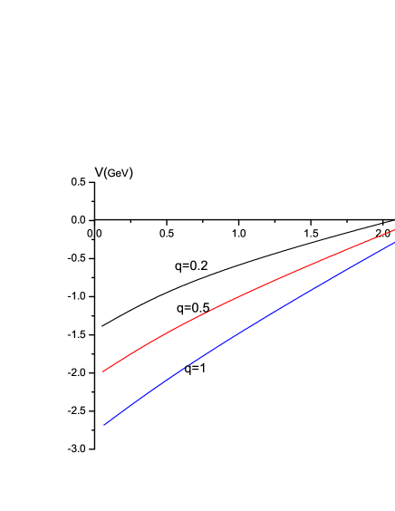
Figure 1: Plots of $V$ versus $L$ with three different values of $q$. Here $T=0.1GeV$. From top to bottom $q=0.2,0.5,1.0$.

Before going further, we would like to discuss the values of some parameters. The coefficient $\frac{1}{\pi\alpha^{\prime}}$ and the AdS radius $R$ do not play any role in the physical discussion, so we set $\frac{1}{\pi\alpha^{\prime}}=2R^{2}=1$, the similar assumption can be found in YS1 . In addition, the value of $q$ is related to the gluon condensation $<TrF^{2}>$ in boundary theory and non-zero $q$ implies that the chiral symmetry is broken BG , but in the present work, we only consider the instanton density $q$ as an external parameter, so we can choose the values of $q$ properly, see also in MD .

To find how the instanton density $q$ affects the heavy quark potential qualitatively. In Fig 1 we plot the potential $V$ as a function of the inter-quark distance $L$ with a fixed temperature $T=0.1GeV$ for three different values of $q$. In the plots from top to bottom $q=0.2,0.5,1.0$, respectively. From the figures, we can see clearly that the potential decreases as $q$ increases. Also, one finds that by increasing $q$ the dissociation length increases. Therefore, the instanton density tends to suppress the heavy quark potential as well as make the dissociation length longer. Interestingly, some other corrections such as the sub-leading order corrections ZQ and the higher curvature corrections KB1 both make the dissociation length shorter.

IV jet quenching parameter

Next, we investigate the jet quenching parameter in this D-instanton background. The eikonal approximation relates the jet quenching parameter with the expectation value of an adjoint Wilson loop $W^{A}[{\cal C}]$, where ${\cal C}$ is a rectangular contour of size $L\times L_{-}$, the sides with length $L_{-}$ run along the light-cone, the limit $L_{-}\to\infty$ is taken in the end. Under the dipole approximation, which is valid for small transverse separation $L$, the jet quenching parameter defined in Ref RB can be extracted from the asymptotic expression for $TL<<1$

$$<W^{A}[{\cal C}]>\approx\exp[-\frac{1}{4\sqrt{2}}\hat{q}L_{-}L^{2}],$$ (26)

where $<W^{A}[{\cal C}]>\approx<W^{F}[{\cal C}]>^{2}$ with $<W^{F}[{\cal C}]>$ the thermal expectation value in the fundamental representation.

Using the AdS/CFT correspondence, one can calculate $<W^{F}[{\cal C}]>$ according to:

$$<W^{F}[{\cal C}]>\approx\exp[-S_{I}],$$ (27)

with $S_{I}=S-S_{0}$, where $S$ is the total energy of the quark pair, $S_{0}$ is the self-energy of the isolated quark and the isolated anti-quark.

Thus, the general relation for the jet quenching parameter can be written as

$$\hat{q}=8\sqrt{2}\frac{S_{I}}{L_{-}L^{2}}.$$ (28)

By virtue of the light-cone coordinate $x^{\mu}=(r,x^{+},x^{-},x_{2},x_{3})$, the metric Eq.(2) becomes

$$ds^{2}=-e^{\frac{\Phi}{2}}\frac{r^{2}}{R^{2}}(1+f)dx^{+}dx^{-}+e^{\frac{\Phi}{2}}\frac{r^{2}}{R^{2}}(dx_{2}^{2}+dx_{3}^{2})+e^{\frac{\Phi}{2}}\frac{1}{2}\frac{r^{2}}{R^{2}}(1-f)[(dx^{+})^{2}+(dx^{-})^{2}]+e^{\frac{\Phi}{2}}\frac{R^{2}}{r^{2}f}dr^{2}.$$ (29)

As the Wilson loop in question stretches across $x_{2}$ and lies at $x^{+}=constant,x_{3}=constant$, we can choose the static gauge as

$$x^{-}=\tau,\qquad x_{2}=\sigma,$$ (30)

and suppose a profile of $r=r(\sigma)$, then Eq.(29) becomes

$$ds^{2}=e^{\frac{\Phi}{2}}[\frac{1}{2}(\frac{r^{2}}{R^{2}}-f_{1})d\tau^{2}+(\frac{r^{2}}{R^{2}}+\frac{\dot{r}^{2}}{f_{1}})d\sigma^{2}],$$ (31)

where $\dot{r}=\frac{dr}{d\sigma}$, $f_{1}\equiv\frac{r^{2}}{R^{2}}(1-\frac{r_{t}^{4}}{r^{4}})$.

Then the Nambu-Goto action is given by

$$S=\frac{\sqrt{2}L_{-}}{2\pi\alpha^{\prime}}\int_{0}^{\frac{L}{2}}d\sigma\sqrt{e^{\Phi}(\frac{r^{2}}{R^{2}}-f_{1})(\frac{r^{2}}{R^{2}}+\frac{\dot{r}^{2}}{f_{1}})},$$ (32)

where the boundary condition is $r(\pm\frac{L}{2})=\infty$.

Note that the integrand doe not depend explicitly on $\sigma$, so we have a conserved quantity

$$\frac{\partial\mathcal{L}}{\partial\dot{r}}\dot{r}-\mathcal{L}=\frac{-e^{\Phi}(\frac{r^{2}}{R^{2}}-f_{1})\frac{r^{2}}{R^{2}}}{\sqrt{e^{\Phi}(\frac{r^{2}}{R^{2}}-f_{1})(\frac{r^{2}}{R^{2}}+\frac{\dot{r}^{2}}{f_{1}})}}=C,$$ (33)

which leads to

$$\dot{r}^{2}=\frac{f_{1}r^{2}}{R^{2}C^{2}}[\frac{e^{\Phi}r^{2}(\frac{r^{2}}{R^{2}}-f_{1})}{R^{2}}-C^{2}].$$ (34)

The above Eq.(34) involves determining the zeros and the region of positivity of the right-hand side. It was argued liu that the turning point occurs at $f_{1}=0$, implying $\dot{r}=0$ at the horizon $r=r_{t}$.

As a matter of convenience, we set $B\equiv\frac{1}{C^{2}}$. For the low energy limit ($C\rightarrow 0$), one can integrate Eq.(34) to leading order in $\frac{1}{B}$ and obtain the following relation

$$L=2R^{2}\int_{r_{t}}^{\infty}dr\sqrt{\frac{1}{(\frac{r^{2}}{R^{2}}-f_{1})Bf_{1}r^{4}e^{\Phi}}}.$$ (35)

On the other hand, plugging Eq.(34) into Eq.(32), one can rewrite the Nambu-Goto action as follows:

$$S = \frac{\sqrt{2}L_{-}}{2\pi\alpha^{\prime}}\int_{r_{t}}^{\infty}dr\sqrt{\frac{e^{2\Phi}(\frac{r^{2}}{R^{2}}-f_{1})^{2}r^{2}}{f_{1}[e^{\Phi}r^{2}(\frac{r^{2}}{R^{2}}-f_{1})-R^{2}C^{2}]}}$$ (36)

$$= \frac{\sqrt{2}L_{-}\sqrt{B}}{2\pi\alpha^{\prime}}\int_{r_{t}}^{\infty}dr\frac{e^{\Phi}(\frac{r^{2}}{R^{2}}-f_{1})r}{\sqrt{e^{\Phi}(\frac{r^{2}}{R^{2}}-f_{1})Bf_{1}r^{2}-f_{1}R^{2}}}.$$

Likewise, we expand Eq.(36) to leading order of $\frac{1}{B}$,

$$S=\frac{\sqrt{2}L_{-}}{2\pi\alpha^{\prime}}\int_{r_{t}}^{\infty}dr[1+\frac{R^{2}}{2e^{\Phi}(\frac{r^{2}}{R^{2}}-f_{1})Br^{2}}]\sqrt{\frac{1}{f_{1}}e^{\Phi}(\frac{r^{2}}{R^{2}}-f_{1})}.$$ (37)

This action needs to be subtracted by the self energy of the two quarks, that is

$$S_{0} = \frac{2L_{-}}{2\pi\alpha^{\prime}}\int_{r_{t}}^{\infty}dr\sqrt{g_{--}g_{rr}}$$ (38)

$$= \frac{\sqrt{2}L_{-}}{2\pi\alpha^{\prime}}\int_{r_{t}}^{\infty}dr\sqrt{\frac{1}{f_{1}}e^{\Phi}(\frac{r^{2}}{R^{2}}-f_{1})}.$$

The subtracted action is therefore:

$$S_{I}=S-S_{0}=\frac{\sqrt{2}L_{-}R^{2}}{4\pi\alpha^{\prime}B}\int_{r_{t}}^{\infty}dr\sqrt{\frac{1}{(\frac{r^{2}}{R^{2}}-f_{1})f_{1}r^{4}e^{\Phi}}}.$$ (39)

Thus, from Eq.(28), Eq.(35) and Eq.(39), we can obtain the jet quenching parameter in a D-instanton background

$$\hat{q}=\frac{J(q)^{-1}}{\pi\alpha^{\prime}},$$ (40)

where

$$J(q)=R^{2}\int_{r_{t}}^{\infty}dr\sqrt{\frac{1}{(\frac{r^{2}}{R^{2}}-f_{1})f_{1}r^{4}e^{\Phi}}}.$$ (41)

Note that one can recover the jet quenching parameter of $N=4$ SYM theory liu by plugging the instanton density $q=0$ in Eq.(40).

Numerically, we plot the curve of $\hat{q}/\hat{q}_{SYM}$ in terms of the instanton density $q$ at a fixed temperature in Fig 2. The plot shows that the jet quenching parameter in a D-instanton background is larger than that of $N=4$ SYM theory. Also we find that the jet quenching parameter increases as the instanton density increases. This result is in agreement with that in JF which argues that for $\mathcal{N}=4$ SYM theory certain marginal deformations have the effect of enhancing $\hat{q}$.

Furthermore, we would like to compare the results with experimental data. Before going on, we should discuss the values for $\alpha^{\prime}$ and $\lambda$ at hand. We here take $\alpha^{\prime}=0.5$, which is reasonable for temperatures not far above the QCD phase transition liu . In addition, the typical interval of $\lambda$ is $5.5<\lambda<6\pi$ GB1 . We now use $\alpha^{\prime}=0.5$, $\lambda=6\pi$ and $T=300Mev$ to make estimates. From Eq.(40), we find $\hat{q}=5.0,5.31,5.58GeV^{2}/fm$ for $q=1,2,3$. These values of the jet quenching parameter are consistent with the extracted values from RHIC data($5\to 25GeV^{2}/fm$) JD .

Figure 2: Plots of $\hat{q}/\hat{q}_{SYM}$ versus instanton density q at a fixed temperature. Here $T=300Mev$

V conclusion and discussion

In this paper, we have investigated the heavy quark potential and the jet quenching parameter in a D-instanton background. The dual gravitational theory is related to a near horizon limit of stack of black D3-branes with homogeneously distributed D-instantons. Although the theory is not directly applicable to QCD, the features of D3-D(-1) configuration is similar to QCD. Thus, one can expect the results obtained from this theory should shed qualitative insights into analogous questions in QCD.

In section III, we have investigated the heavy quark potential in this D-instanton background. The potential was obtained by calculating the Nambu-Goto action of string attaching the rectangular Wilson loop. It is shown that the presence of instantons tends to suppress the heavy quark potential and increase the dissociation length.

In section IV, the jet quenching parameter has been studied in this D-instanton background as well. It is found that the nonzero instanton density has the effect of enhancing the jet quenching parameter. Also, after taking some proper values of $\alpha^{\prime}$ and $\lambda$, we observe that the results are consistent with the experimental data.

Finally, it is interesting to note that the instanton effects on the heavy-quark potential has also been studied from lattice QCD recently BT .

VI Acknowledgments

This research is partly supported by the Ministry of Science and Technology of China (MSTC) under the 973 Project no. 2015CB856904(4). Zi-qiang Zhang is supported by the NSFC under Grant no. 11547204. Gang Chen is supported by the NSFC under Grant no. 11475149. De-fu Hou is partly supported by the NSFC under Grant nos. 11375070, 11221504 and 11135011.

References

- (1) J. Adams et al. [STAR Collaboration], Nucl. Phys. A 757, 102 (2005).
- (2) K. Adcox et al. [PHENIX Collaboration], Nucl. Phys. A 757, 184 (2005).
- (3) E. V. Shuryak, Nucl. Phys. A 750, 64 (2005).
- (4) J. M. Maldacena, Adv. Theor. Math. Phys. 2, 231 (1998) [Int. J. Theor. Phys. 38, 1113 (1999).
- (5) S. S. Gubser, I. R. Klebanov and A. M. Polyakov, Phys. Lett. B428, 105 (1998).
- (6) O. Aharony, S. S. Gubser, J. Maldacena, H. Ooguri and Y. Oz, Phys. Rept. 323, 183 (2000).
- (7) J. M. Maldacena, Phys. Rev. Lett 80, 4859 (1998).
- (8) A. Brandhuber, N. Itzhaki, J. Sonnenschein and S. Yankielowicz, Phys. Lett. B 434, 36 (1998).
- (9) S. J. Rey, S. Theisen and J. T. Yee, Nucl. Phys. B 527, 171 (1998).
- (10) Y. Kinar, E. Schreiber and J. Sonnenschein, Nucl. Phys. B 566, 103 (2000).
- (11) S.-x. Chu, D. Hou and H.-c. Ren, JHEP 08, 004 (2009).
- (12) Z.-q. Zhang, D. Hou, H.-c Ren and L. Yin, JHEP 1107 035 (2011).
- (13) O. Andreev and V. I. Zakharov, JHEP 0704 100 (2007).
- (14) S. He, M. Huang, Q.-s. Yan, Prog. Theor. Phys. Suppl 186 504 (2010).
- (15) S. He, M. Huang, Q.-s. Yan, Phys.Rev.D 83 045034 (2011)
- (16) J. Greensite and P. Olesen, JHEP 9808, 009 (1998).
- (17) F. Bigazzi, A. L. Cotrone, L. Martucci and L. A. Pando Zayas, Phys. Rev. D 71, 066002 (2005).
- (18) L. Martucci, Fortsch. Phys. 53, 936 (2005).
- (19) K. Bitaghsir Fadafan, Eur. Phys. J. C 71 1799 (2011) [hep-ph/1102.2289].
- (20) R. Baier, Y. L. Dokshitzer, A. H. Mueller, S. Peigne and D. Schiff, Nucl. Phys. B 484, 265 (1997) [hep-ph/9608322].
- (21) M. Gyulassy, I. Vitev, X.-N. Wang, B.-W. Zhang, [nucl-th/0302077].
- (22) H. Liu, K. Rajagopal and U. A. Wiedemann, Phys. Rev. Lett. 97, 182301 (2006) [hep-ph/0605178].
- (23) K. J. Eskola, H. Honkanen, C.A. Salgado, U.A. Wiedemann, Nucl. Phys. A 747, 511 (2005) [hep-ph/0406319].
- (24) A. Dainese, C. Loizides and G. Paic, Eur. Phys. J. C 38 461 (2005) [hep-ph/0406201].
- (25) Z. -q. Zhang, D. -f. Hou and H. -C. Ren, JHEP 1301 032 (2013) [hep-th/1210.5187].
- (26) K. B. Fadafan, Eur. Phys. J. C 68 505 (2010) [hep-th/0809.1336].
- (27) F. -l. Lin, T. Matsuo, Phys.Lett.B 641:45-49,(2006) [hep-th/0606136].
- (28) N. Armesto, J. D. Edelstein and J. Mas, JHEP 0609 039 (2006) [hep-ph/0606245].
- (29) S. D. Avramis, K. Sfetsos, JHEP 0701 065 (2007) [hep-ph/0606245].
- (30) K. B. Fadafan, B. Pourhassan and J. Sadeghi, Eur. Phys. J. C 71:1785 (2011) [hep-th/1005.1368].
- (31) E. Nakano, S. Teraguchi and W.Y. Wen, Phys.Rev.D 75:085016 (2007) [hep-th/0608274].
- (32) U. G rsoy, E. Kiritsis, G. Michalogiorgakis and F. Nitti, JHEP 0912 056 (2009) [hep-ph/0906.1890].
- (33) A. Ficnar, S. S. Gubser and M. Gyulassy, Phys. Lett. B 738 464(2014) [hep-ph/1311.6160].
- (34) A. Buchel, Phys. Rev. D74 046006 (2006) [hep-th/0605178].
- (35) J. F. Vazquez-Poritz, [hep-th/0605296].
- (36) E. Caceres and A. Guijosa, JHEP 0612 068,(2006) [hep-th/0606134].
- (37) H. Liu, K. Rajagopal and U. A. Wiedemann, Phys. Rev. Lett. 98 182301 (2007) [hep-ph/0605178].
- (38) M. Benzke, N. Brambilla, M. A. Escobedo and A. Vairo, JHEP 1302 (2013) 129.
- (39) Z. -q. Zhang, D. -f. Hou, Y. Wu and G. Chen, Advances in High Energy Physics, Volume 2016 (2016), Article ID9503491.
- (40) N. Dorey, T. J. Hollowood, V. V. Khoze, and M. P. Mattis, Phys. Rep. 371 (2002) 231 [hep-th/0206063].
- (41) O. Aharony, S. S. Gubser, J. Maldacena, H. Ooguri, and Y. Oz, Phys. Rep. 323 (2000) 183 [hep-th/9905111].
- (42) L. Hong and A. A. Tseytlin, Nuc. Phys. B 553 (1999) 231 [hep-th/9903091].
- (43) B. Gwak, M. Kim, B.-H. Lee, Y. Seo, and S.-J. Sin, Phys. Rev. D 86 (2012) 026010 [hep-th/1203.4883].
- (44) K. Ghoroku, T. Sakaguchi, N. Uekusa, and M. Yahiro, Phys. Rev. D 71 (2005) 106002 [hep-th/0502088].
- (45) G. W. Gibbons, M. B. Green and M. J. Perry, Phys. Lett. B 370, 37 (1996) [hep-th/9511080].
- (46) A. Kehagias and K. Sfetsos, Phys. Lett. B 456, 22 (1999) [hep-th/9903109].
- (47) Y. Sato and K. Yoshida, JHEP 1309 (2013) 134 [hep-th/1306.5512].
- (48) M. Dehghani and P. Dehghani, [hep-th/1511.07986].
- (49) S.Gubser, Phys. Rev. D 76, (2007) 126003.
- (50) J. D. Edelstein and C. A. Salgado, AIP Conf. Proc. 1031 (2008) 207-220, [hep-ph/0805.4515].
- (51) B. Turimov, H. Kim, U. Yakhshiev, M. M. Musakhanov and E. Hiyama, [hep-lat/1602.06074].