Quasinonlocal coupling of nonlocal diffusions

Abstract.

We developed a new self-adjoint, consistent, and stable coupling strategy for nonlocal diffusion models, inspired by the quasinonlocal atomistic-to-continuum method for crystalline solids. The proposed coupling model is coercive with respect to the energy norms induced by the nonlocal diffusion kernels as well as the $L^{2}$ norm, and it satisfies the maximum principle. A finite difference approximation is used to discretize the coupled system, which inherits the property from the continuous formulation. Furthermore, we design a numerical example which shows the discrepancy between the fully nonlocal and fully local diffusions, whereas the result of the coupled diffusion agrees with that of the fully nonlocal diffusion.

1. Introduction

Nonlocal models have been developed and received lot of attention in recent years to model systems with important scientific and engineering applications, for example, the phase transition [2, 14], the nonlocal heat conduction [4], the peridynamics model for mechanics [33], just to name a few. These nonlocal models give rise to new questions and challenges to applied mathematics both in terms of analysis and numerical algorithms.

While it is established that the nonlocal formulations can often provide more accurate descriptions of the systems, the nonlocality also increases the computational cost compared to conventional models based on PDEs. As a result, methodologies that couple nonlocal models with more localized descriptions have been investigated in recent years. The goal is to combine the accuracy of nonlocal models with the computational and modeling efficiency of local PDEs. The basic idea is to apply the nonlocal model to those parts of the domain that require the improved accuracy, and use the more efficient local PDE model in other regions to reduce the computational costs. Besides, from a modeling point of view, the nonlocal models usually give rise to modeling challenges near the boundary, as volumetric boundary conditions are needed and those are often hard to characterize or match with the physical setup of the system. It is often easier to switch to the local models near the boundary so that usual boundary conditions can be used. Coupling different nonlocal models is also important as it has applications in modeling hierarchically structured materials [40, 16], nonlocal heat conductors [4, 7], etc.

In the past decades, many works have been developed for numerical analysis of nonlocal models, for example [6, 9, 10, 11, 20, 36], which gave understanding to properties and asymptotic behaviors. In particular, many strategies are proposed to couple together local-to-nonlocal or two nonlocal models with different nonlocality. For example, (1) Arlequin type domain decomposition, see e.g., [28, 17]; (2) Optimal-control based coupling, e.g., [8, 7]; (3) Morphing approach as in [23]; (4) Force-based blending mechanism, see e.g., [29, 30]; (5) Energy-based blending mechanism, see e.g., [35, 12], just to name a few.

Nonlocal models are considered as top-down continuum approaches which use integral formulations to represent nonlocal spatial interactions [18, 19, 33]. Within a nonlocal model, each material point interacts through short-range forces with other points inside a horizon of prescribed radius $\delta$, which leads to a nonlocal integral-type continuum theory [33]. Complementary to top-down nonlocal continuum approaches are bottom-up atomistic-to-continuum (AtC) approaches, which give atomistic accuracy near defects such as crack tips and continuum finite element efficiency elsewhere. Notice that top-down nonlocal models and bottom-up AtC models actually share a lot interconnections (see for example, [3, 15, 16, 22] for more discussions). Many of the coupling strategies developed for nonlocal models were also inspired or connected to those of AtC coupling methods for crystalline materials (see e.g., the review articles [24, 25]). The AtC coupling can be indeed understood as a nonlocal-local coupling as well, since the atomistic models typically involve interactions of atoms within the interaction range (i.e., horizon) which are beyond the nearest neighbor. Additionally, the nonlocal models and AtC models have some similarities in one-dimension after finite difference discretization.

In fact, the coupling strategy we proposed in this work also borrows the idea of quasinonlocal coupling [32, 13] which was developed in the context of AtC method, and a detailed interpretation of quasinonlocal coupling will be given in section 3. The proposed method gives a self-adjoint coupling kernel in the divergence form using the terminology of [5]. In physics terms, the coupling naturally satisfies the Newton’s third law since the coupling is done on the energy level. Moreover, the coupling we proposed satisfies the patch-test consistency, $L^{2}$ stability, and the maximum principle. As far as we know, none of existing coupling strategies satisfies all these properties. We believe the coupling strategy is more advantageous over the existing methods.

The paper is organized as follows. In section 2, we give a brief review of nonlocal diffusion problem. In section 3, we propose the quasinonlocal coupling, and prove it is self-adjoint and patch-test consistent. In addition, we prove that the quasinonlocal diffusion is positive-definite with respect to the energy norm induced by the nonlocal diffusion kernels as well as the $L^{2}$ norm, and it satisfies the maximum principle. In section 4, we provide a first order finite difference approximation for the purpose of numerical implementation, which keeps the properties of continuous level. In section 5, we verify our theoretical results by a few numerical examples.

2. The nonlocal diffusion

We first review the definition and properties of the nonlocal diffusion problem, following mainly the notations in [9, 10]. Consider an open domain $\Omega\subset\mathbb{R}^{d}$ and for $u(x):\,\mathbb{R}^{d}\to\mathbb{R}$, the (linear) nonlocal diffusion operator $\mathcal{L}_{\delta}$ is defined as

$$\mathcal{L}_{\delta}u(x):=\int_{\mathbb{R}^{d}}\left(u(y)-u(x)\right)\gamma_{\delta}(x,y)dy,\quad\forall x\in\Omega,$$ (1)

where $\delta$ is the horizon parameter and $\gamma_{\delta}(x,y):\mathbb{R}^{d}\times\mathbb{R}^{d}\rightarrow\mathbb{R}$ denotes a nonnegative symmetric function. Under the assumption of translational invariance and isotropy, the kernel $\gamma_{\delta}(x,y)$ reduces to a radial function depending on the distance $|x-y|$ and is given by[34]

$$\gamma_{\delta}(x,y)=\gamma_{\delta}({\lvert x-y\rvert})=\frac{1}{\delta^{d+2}}\gamma\left(\frac{{\lvert x-y\rvert}}{\delta}\right),$$ (2)

where $d$ is the spatial dimension and $\gamma$ is a non-negative radially symmetric nonlocal diffusion kernel which satisfies

• Translational invariance and isotropy: $\gamma(x,y)=\gamma(\lvert y-x\rvert)\geq 0$;

• Compact support: $\gamma(x,y)=0$ if $\lvert x-y\rvert\geq 1$;

• Finite second moment: $\int s^{2}\gamma(s)ds<\infty$. Note that due to the scaling choice in (2), the second moment is scale invariant, i.e., $\int s^{2}\gamma_{\delta}(s)ds$ takes the same value for any $\delta$.

With Dirichlet boundary condition, the initial-boundary value problem for the nonlocal diffusion is then given by:

$$\begin{cases}\displaystyle\frac{\partial u_{n}}{\partial t}=\mathcal{L}_{\delta}u_{n}(x)=\int_{B_{\delta}(x)}\left(u_{n}(y)-u_{n}(x)\right)\gamma_{\delta}(x,y)dy,\quad\forall x\in\Omega,\,\forall t>0\\ u_{n}(x,t)=0,\quad\forall x\in\Omega_{\mathcal{I}},\,\forall t\geq 0,\\ u_{n}(x,0)=u_{n}^{0}(x),\quad\forall x\in\Omega,\end{cases}$$ (3)

where the subscript in $u_{n}$ stands for “nonlocal” and $\Omega_{\mathcal{I}}=\mathbb{R}^{d}\backslash\Omega$ is known as the interaction domain [11], on which the volumetric Dirichlet boundary condition is imposed on $u_{n}$. Since the kernel $\gamma_{\delta}(x,y)$ is zero if $\lvert x-y\rvert>\delta$, we have restricted the integration (3) in $B_{\delta}(x)$: the $\delta$-ball around $x$ and also the interaction domain $\Omega_{\mathcal{I}}$ can be also restricted to the $\delta$-neighborhood of $\Omega$:

$$\Omega_{\mathcal{I}}:=\{y\in\mathbb{R}^{d}\setminus\Omega:|y-x|{\leq}\delta\text{ for some }x\in\Omega\}.$$ (4)

Other boundary conditions can be used, for example if $\Omega$ is a box region $\Omega=[0,L)^{d}$, we can impose the periodic boundary conditions on $u_{n}$. The corresponding initial-boundary value problem can be written down analogously.

The nonlocal diffusion operator is associated with the Hilbert spaces given by

$$S_{\delta}:=\left\{u\in L^{2}(\Omega\cup\Omega_{\mathcal{I}}):\int_{\Omega\cup\Omega_{\mathcal{I}}}\int_{\Omega\cup\Omega_{\mathcal{I}}}\gamma_{\delta}(x,y)\left(u(y)-u(x)\right)^{2}dxdy<\infty,\;u\big{|}_{\Omega_{\mathcal{I}}}=0\right\}.$$

The induced nonlocal energy norm is denoted as $\|\cdot\|_{S_{\delta}}$:

$$\|u\|_{S_{\delta}}^{2}:=\int_{\Omega\cup\Omega_{\mathcal{I}}}\int_{\Omega\cup\Omega_{\mathcal{I}}}\gamma_{\delta}(x,y)\left(u(y)-u(x)\right)^{2}dxdy,\quad\forall u\in S_{\delta}.$$ (5)

The properties of the nonlocal kernel as well as the nonlocal energy norms are investigated and discussed in many recent works, we refer the readers to [10, 37, 36, 7] and references therein. We remark in particular that the nonlocal energy norm satisfies the nonlocal Poincaré inequality [7, Eq. (2.11)], which will be used in our analysis in the sequel:

$$\|u\|_{L^{2}(\Omega\cup\Omega_{\mathcal{I}})}\leq C_{d,\delta}\|u\|_{S_{\delta}}.$$ (6)

The horizon parameter should be chosen according the physical property of the underlying system. We are interested in the cases where the horizon parameter changes across the domain of interest. In this case, we shall couple two nonlocal diffusion operators with different horizon parameters together. In the next section, we propose a way of coupling based on the quasinonlocal idea. While we focus in this work the coupling of two nonlocal diffusions, we note that the idea can be extended to coupling of local and nonlocal diffusions, which will be considered in future works.

3. The quasinonlocal coupling

In this section, we propose a coupling scheme for multiscale nonlocal diffusions, and prove the consistency, $L^{2}$ stability and the maximum principle for the new coupling operator.

To better convey the idea, we will limit our discussion to one dimensional case in this work. For simplicity of notation, we assume that $\Omega=[-a,b]$ and it is divided into two parts $\Omega_{1}=[-a,0]$ and $\Omega_{2}=[0,b]$ with the interface at $0$. We assume that within $\Omega_{1}$, the nonlocal diffusion kernel $\gamma_{\delta_{1}}$ should be employed and $\gamma_{\delta_{2}}$ should be used in $\Omega_{2}$. Without loss of generality, we assume $\delta_{1}>\delta_{2}$ and thus $\Omega_{1}$ is a more nonlocal region compared to $\Omega_{2}$. We further assume that $\delta_{1}=M\delta_{2}$ with $M\in\mathbb{N}$ being an integer. Our coupling strategy requires $M$ to be an integer; it might be interesting to study how to extend to arbitrary ratio of $\delta_{1}$ and $\delta_{2}$.

To ensure the symmetry, we will derive the coupled nonlocal diffusion operator (i.e., negative of the force) from a total energy. Recall that the total energy associated with the kernel $\gamma_{\delta}$ is

$$E^{{\mathsf{tot}},\delta}(u)=\frac{1}{4}\int_{\mathbb{R}}\int_{\mathbb{R}}\gamma_{\delta}(\lvert y-x\rvert)\left(u(y)-u(x)\right)^{2}~{}dxdy.$$ (7)

An intuitive coupling idea is to combine the energies associated with $\delta_{1}$ and $\delta_{2}$, respectively. For instance, we use $\gamma_{\delta_{2}}$ if $x,y\in\Omega_{2}$ and $\gamma_{\delta_{1}}$ otherwise. It can be verified though, such coupling strategy does not satisfy the patch-test consistency. The resulting operator (as the first variation of the energy) $\mathcal{L}$ does not annihilate affine functions, which is of course a property one would hope a diffusion operator should satisfy.

3.1. Quasinonlocal coupling with geometric reconstruction

To overcome the difficulty of naive coupling strategies, our construction does not simply try to vary $\delta$ in (7) across the domain, but instead, we follow the geometric reconstruction reformulation for the quasinonlocal method [13]. Let us first present the formulation of the coupling before explaining the ideas behind. Our proposed total energy of the quasinonlocal coupling is given by

$$E^{{\mathsf{tot}},{\mathsf{qnl}}}(u)= \frac{1}{4}\int_{x,y\in\mathbb{R},x\leq 0\text{ or }y\leq 0}\gamma_{\delta_{1}}(\lvert y-x\rvert)\left(u(y)-u(x)\right)^{2}~{}dx~{}dy$$ (8)

$$\;+\frac{1}{4}\int_{x,y\in\mathbb{R},x>0\text{ and }y>0}\gamma_{\delta_{1}}(\lvert y-x\rvert)$$

$$\;\;\cdot\frac{1}{M}\sum_{j=0}^{M-1}\left(u(x+\frac{j+1}{M}(y-x))-u(x+\frac{j}{M}(y-x))\right)^{2}\,M^{2}~{}dx~{}dy.$$

Note that the energy functional only uses one interaction kernel $\gamma_{\delta_{1}}$ (the more non-local one) throughout the entire domain $\Omega=\Omega_{1}\cup\Omega_{2}$. In the subregion $\Omega_{2}$, instead of changing to the kernel $\gamma_{\delta_{2}}$, we change the difference $(u(y)-u(x))^{2}$ to an averaged version. This is coined as “geometric reconstruction”, since it reconstructs $u(y)-u(x)$ by differences of $u$ evaluated at points that are at most of distance $\delta_{2}$ to each other. Therefore, while a longer range kernel $\gamma_{\delta_{1}}$ is used in $\Omega_{2}$, the energy effectively still only involves interaction no further than $\delta_{2}$ distance. More concretely, to link the regions from kernel $\gamma_{\delta_{1}}$ to $\gamma_{\delta_{2}}$ with $\delta_{1}=M\delta_{2}$, in the local region $\Omega_{2}$, we replace ${{\gamma_{\delta_{2}}}}(\lvert y-x\rvert)\left(u(y)-u(x)\right)^{2}$ by (see Figure 1 for an illustration)

$$\gamma_{\delta_{1}}(\lvert y-x\rvert)\frac{1}{M}\sum_{j=0}^{M-1}\left(u\bigl{(}x+\frac{j+1}{M}(y-x)\bigr{)}-u\bigl{(}x+\frac{j}{M}(y-x)\bigr{)}\right)^{2}\left(\frac{\delta_{1}}{\delta_{2}}\right)^{2}\\ =\gamma_{\delta_{1}}(\lvert y-x\rvert)\frac{1}{M}\sum_{j=0}^{M-1}\left(u\bigl{(}x+\frac{j+1}{M}(y-x)\bigr{)}-u\bigl{(}x+\frac{j}{M}(y-x)\bigr{)}\right)^{2}\,M^{2}.$$

Note that the kernel remains intact, and we adopt the geometric reconstruction to replace

$$u(y)-u(x)\rightarrow\left(u\bigl{(}x+\frac{j+1}{M}(y-x)\bigr{)}-u\bigl{(}x+\frac{j}{M}(y-x)\bigr{)}\right)M$$

for $j=0,\ldots,M-1$ and average the modulus square of the result over the $M$ possibilities. Note that if $\lvert x-y\rvert\leq\delta_{1}$, the difference on the right is $u$ evaluated at points with distance at most $\frac{\delta_{1}}{M}=\delta_{2}$; thus effectively we reconstruct the difference $u(y)-u(x)$ by a more local interaction (and hence the idea was referred as geometric reconstruction scheme in [13]). In fact, if we adopt such reconstruction everywhere in the computational domain, we will get the nonlocal diffusion with the kernel $\gamma_{\delta_{2}}$, as shown in the following Proposition.

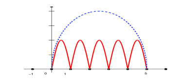
Figure 1. An example of quasinonlocal construction in one dimension: $x\leq 0$ is the region with kernel $\gamma_{\delta_{1}}$ and $x>0$ is the region with kernel $\gamma_{\delta_{2}}$ ($M=5$). The blue dash bond representing the difference $u(y)-u(x)$ is geometrically reconstructed by the red solid bonds with length at most $\delta_{2}$.

Proposition 3.1.

The energy functional defined on the entire domain $\Omega\cup\Omega_{\mathcal{I}}$ with geometric reconstruction

$$E^{{\mathsf{tot}},{\mathsf{gr}}}(u):=\frac{1}{4} \int_{x,y\in\Omega\cup\Omega_{\mathcal{I}}}\gamma_{\delta_{1}}(\lvert y-x\rvert)$$ (9)

$$\frac{1}{M}\sum_{j=0}^{M-1}\left(u\left(x+\frac{j+1}{M}(y-x)\right)-u\left(x+\frac{j}{M}(y-x)\right)\right)^{2}M^{2}~{}dxdy$$

is equivalent to the total nonlocal energy with diffusion kernel $\gamma_{\delta_{2}}$:

$$E^{{\mathsf{tot}},\delta_{2}}(u):= \frac{1}{4}\int_{x,y\in\Omega\cup\Omega_{\mathcal{I}}}\gamma_{\delta_{2}}(\lvert y-x\rvert)\left(u(y)-u(x)\right)^{2}~{}dxdy.$$

Proof.

Outside the support, the diffusion kernel is zero, and because of the zero volumetric Dirichlet boundary condition, so the total energy (9) can be recast as an integral of entire real line $\mathbb{R}$:

$$E^{{\mathsf{tot}},{\mathsf{gr}}}(u) \,=\frac{1}{4}\int_{x,y\in\mathbb{R}}M\gamma_{\delta_{1}}(\lvert y-x\rvert)$$

$$\sum_{j=0}^{M-1}\left(u\left(x+\frac{j+1}{M}(y-x)\right)-u\left(x+\frac{j}{M}(y-x)\right)\right)^{2}~{}dxdy.$$ (10)

For each fixed $0\leq j\leq M-1$ in (3.1), we introduce change of variables

$$z:=x+\frac{j+1}{M}(y-x)=\left(1-\frac{j+1}{M}\right)x+\frac{j+1}{M}y$$

to replace $y$, thus we obtain

$$\begin{split}\frac{1}{4}&\int_{x,y\in\mathbb{R}}M\gamma_{\delta_{1}}(\lvert y-x\rvert){{\left(u\left(x+\frac{j+1}{M}(y-x)\right)-u\left(x+\frac{j}{M}(y-x)\right)\right)^{2}}}~{}dxdy\\ =&\frac{1}{4}\int_{x,z\in\mathbb{R}}\gamma_{\delta_{1}}\left(\frac{M}{j+1}\lvert z-x\rvert\right)\frac{M^{2}}{j+1}\left(u\left(z\right)-u\left(z-\frac{1}{j+1}(z-x)\right)\right)^{2}~{}dzdx\\ =&\frac{1}{4}\int_{x,z\in\mathbb{R}}\frac{1}{M^{3}}\gamma_{\delta_{2}}\left(\frac{1}{j+1}\lvert z-x\rvert\right)\frac{M^{2}}{j+1}\left(u\left(z\right)-u\left(z-\frac{1}{j+1}(z-x)\right)\right)^{2}~{}dzdx.\end{split}$$

Next, let $w=z-\frac{1}{j+1}(z-x)=z+\frac{1}{j+1}(x-z)$ to replace $x$, we further get

$$\begin{split}\frac{1}{4}\int_{x,z\in\mathbb{R}}&\frac{1}{M^{3}}\gamma_{\delta_{2}}\left(\frac{1}{j+1}\lvert z-x\rvert\right)\frac{M^{2}}{j+1}\left(u\left(z\right)-u\left(z-\frac{1}{j+1}(z-x)\right)\right)^{2}~{}dzdx\\ =&\frac{1}{4}\int_{w,z\in\mathbb{R}}\frac{1}{M}\gamma_{\delta_{2}}\left(\lvert w-z\rvert\right)\left(u\left(z\right)-u\left(w\right)\right)^{2}~{}dzdw=\frac{1}{M}E^{{\mathsf{tot}},\delta_{2}}(u).\end{split}$$

Summing up all $0\leq j\leq M-1$, we proved the proposition. ∎

Therefore, to couple diffusion kernels $\gamma_{\delta_{1}}$ and $\gamma_{\delta_{2}}$ with interface at $x=0$, we construct the total coupled energy by using the geometric reconstruction when $x,y\in\Omega_{2}$ and obtain (8), recalled here

$$\begin{split}E^{{\mathsf{tot}},{\mathsf{qnl}}}(u)=&\frac{1}{4}\int_{x,y\in\mathbb{R},x\leq 0\text{ or }y\leq 0}\gamma_{\delta_{1}}(\lvert y-x\rvert)\left(u(y)-u(x)\right)^{2}~{}dx~{}dy\\ &\quad+\frac{1}{4}\int_{x,y\in\mathbb{R},x>0\text{ and }y>0}\gamma_{\delta_{1}}(\lvert y-x\rvert)\\ &\qquad\cdot\frac{1}{M}\sum_{j=0}^{M-1}\left(u(x+\frac{j+1}{M}(y-x))-u(x+\frac{j}{M}(y-x))\right)^{2}\,M^{2}~{}dx~{}dy.\end{split}$$

Clearly, when $\delta_{1}=\delta_{2}$, we have $M=1$ and thus $E^{{\mathsf{tot}},{\mathsf{qnl}}}(u)=E^{{\mathsf{tot}},\delta_{1}}(u).$

The first variation of the above functional (8) then gives us a coupled diffusion operator, for which we call the quasinonlocal diffusion, denoted by $\mathcal{L}^{{\mathsf{qnl}}}$. After straightforward but somewhat lengthy calculation, which we defer to the appendix, we obtain that

$$\begin{split}&\mathcal{L}^{{\mathsf{qnl}}}u_{\mathsf{qnl}}(x):=-\frac{\delta E^{\mathsf{tot},\mathsf{qnl}}}{\delta u}u_{\mathsf{qnl}}(x)\\ &=\begin{cases}\displaystyle\int_{\mathbb{R}}\left(u_{\mathsf{qnl}}(y)-u_{\mathsf{qnl}}(x)\right)\gamma_{\delta_{1}}(\lvert y-x\rvert)dy,&\text{if }x\leq 0,\\ \displaystyle\int_{x-\delta_{1}<y<0}\left(u_{\mathsf{qnl}}(y)-u_{\mathsf{qnl}}(x)\right)\gamma_{\delta_{1}}(\lvert y-x\rvert)dy\\ \displaystyle\;+{{\frac{1}{M}}}\sum_{j=1}^{M-1}\left[\int_{(x-\frac{1}{j}x)<y<(x+\frac{1}{j}x)}\left(u_{\mathsf{qnl}}(y)-u_{\mathsf{qnl}}(x)\right)\gamma_{\delta_{2}}(\lvert y-x\rvert)\right]dy\\ \displaystyle\quad\;+\frac{1}{M}\int_{(x-\frac{1}{M}x)<y}\left(u_{\mathsf{qnl}}(y)-u_{\mathsf{qnl}}(x)\right)\gamma_{\delta_{2}}(\lvert y-x\rvert)dy,&\text{if }0<x<\delta_{1},\\ \displaystyle\int_{\mathbb{R}}\left(u_{\mathsf{qnl}}(y)-u_{\mathsf{qnl}}(x)\right)\gamma_{\delta_{2}}(\lvert y-x\rvert)dy,&\text{if }x\geq\delta_{1}.\end{cases}\end{split}$$ (11)

Note that in the region $\{x\leq 0\}$, the diffusion is just the nonlocal diffusion with kernel $\gamma_{\delta_{1}}$, while the diffusion kernel is given by $\gamma_{\delta_{2}}$ in the region $\{x\geq\delta_{1}\}$. The region in between $\{0<x<\delta_{1}\}$ can be viewed as a buffer region that connects the two nonlocal diffusion operators. We emphasize that the coupled diffusion operator $\mathcal{L}^{{\mathsf{qnl}}}$ is self-adjoint, as it is derived from the coupled energy (8) and can be easily checked directly from the definition; and hence the operator $\mathcal{L}^{{\mathsf{qnl}}}$ is of divergence form (following the definition in [5]). This is the main motivation behind our construction of the kernel.

The idea of the coupling strategy here is in fact borrowed from the quasinonlocal coupling in the context of atomistic-to-continuum method for crystalline solids, first proposed by [32], generalized and analyzed in [13, 26, 31, 21, 27], in particular the geometric reconstruction point of view [13]. Hence we adopt the name of the quasinonlocal coupling strategy. Actually, as only pairwise interaction is involved in the current context of nonlocal diffusion operators, the coupling is considerably easier than the atomistic-to-continuum coupling for crystals. In particular, the extension of atomistic-to-continuum quasinonlocal coupling to higher dimension for general long range potential is still an open challenge, despite progresses in [13, 31, 27]. While for nonlocal diffusion, we expect the extension should not pose serious difficulties and will be considered in future works.

The initial-boundary value problem for the quasinonlocal coupling is given as below:

$$\begin{cases}\displaystyle\frac{\partial u_{\mathsf{qnl}}}{\partial t}=\mathcal{L}^{{\mathsf{qnl}}}u_{\mathsf{qnl}}(x),\quad\forall x\in\Omega,\\ u_{\mathsf{qnl}}(x,t)=0,\quad\forall x\in\Omega_{\mathcal{I}},\quad\forall t\geq 0,\\ u_{\mathsf{qnl}}(x,0)=u_{\mathsf{qnl}}^{0}(x),\text{ on }\Omega.\end{cases}$$ (12)

We now demonstrate the properties of the quasinonlocal diffusion operator $\mathcal{L}^{{\mathsf{qnl}}}$ in the following subsections.

3.2. Consistency

Lemma 3.1.

The quasinonlocal diffusion operator $\mathcal{L}^{{\mathsf{qnl}}}$ defined in (11) is a self-adjoint operator, and is consistent in the sense that $\mathcal{L}^{\mathsf{qnl}}u=0$ for any affine function $u$.

Proof.

The self-adjointness has been shown above already. To check the consistency, consider an affine function $u(x)=Fx+u_{0}$ with both $F$ and $u_{0}$ being constants. Thus, we have

$$u(y)-u(x)=F(y-x).$$

Plugging this into the definition of $\mathcal{L}^{\mathsf{qnl}}$ (11), we have the following three cases.

1. $x\leq 0$, then

   $$\mathcal{L}^{\mathsf{qnl}}u(x)=\int_{\mathbb{R}}F\left(y-x\right)\gamma_{\delta_{1}}(\lvert y-x\rvert)dy=\int_{\mathbb{R}}Fs\gamma_{\delta_{1}}(\lvert s\rvert)ds=0,$$

   which comes from the symmetry of the kernel.

2. $0<x<\delta_{1}$, then

   $$\begin{split}\mathcal{L}^{\mathsf{qnl}}u(x)=&\int_{x-\delta_{1}<y<0}F\left(y-x\right)\gamma_{\delta_{1}}(\lvert y-x\rvert)dy\\ &\quad+\frac{1}{M}\sum_{j=1}^{M-1}\left[\int_{(x-\frac{1}{j}x)<y<(x+\frac{1}{j}x)}F\left(y-x\right)\gamma_{\delta_{2}}(\lvert y-x\rvert)\right]dy\\ &\qquad\qquad\qquad+\int_{(x-\frac{1}{M}x)<y}\frac{1}{M}F\left(y-x\right)\gamma_{\delta_{2}}(\lvert y-x\rvert)dy.\end{split}$$ (13)

   Because of the symmetry of integral domain and the symmetry of the kernel $\gamma_{\delta_{2}}$, the second term in (13) equals zero. Thus, (13) becomes

   $$\begin{split}&\mathcal{L}^{\mathsf{qnl}}u(x)\\ &=\int_{x-\delta_{1}<y<0}F\left(y-x\right)\gamma_{\delta_{1}}(\lvert y-x\rvert)dy\\ &\qquad\quad+\frac{1}{M}\int_{(x-\frac{1}{M}x)<y}F\left(y-x\right)\gamma_{\delta_{2}}(\lvert y-x\rvert)dy\\ &=\int_{x-\delta_{1}}^{0}F\left(y-x\right)\gamma_{\delta_{1}}(\lvert x-y\rvert)dy\\ &\qquad\quad+\frac{1}{M}\int_{(x-\frac{1}{M}x)<y}F\left(y-x\right)M^{3}\gamma_{\delta_{1}}\left(\lvert M(y-x)\rvert\right)dy\\ &=\int_{-\delta_{1}}^{-x}Fs\gamma_{\delta_{1}}(\lvert s\rvert)ds+\int_{-x}^{\infty}F\hat{s}\gamma_{\delta_{1}}(\lvert\hat{s}\rvert)d\hat{s}=\int_{-\delta_{1}}^{\delta_{1}}Fs\gamma_{\delta_{1}}(\lvert s\rvert)ds=0,\end{split}$$ (14)

   where we introduce the change of variables $s:=y-x$ and $\hat{s}:=M(y-x)$.

3. $x\geq\delta_{1}$, then

   $$\mathcal{L}^{\mathsf{qnl}}u(x)=\int_{\mathbb{R}}F\left(y-x\right)\gamma_{\delta_{2}}(\lvert y-x\rvert)dy=\int_{\mathbb{R}}Fs\gamma_{\delta_{2}}(\lvert s\rvert)ds=0,$$

   which again comes from the symmetry of the kernel.

Summarizing all the three cases, we thus obtain the patch-test consistency of the coupled diffusion operator $\mathcal{L}^{\mathsf{qnl}}$. ∎

3.3. Stability analysis of QNL coupling

Let us now consider the stability of the QNL coupling (12) and (11). As the coupled diffusion operator $\mathcal{L}^{\mathsf{qnl}}$ is derived from the total energy (8), the bilinear form of the QNL coupling operator is simply given by

$$b_{\mathsf{qnl}}(u,v)= \int_{x,y\in\mathbb{R},x\leq 0\text{ or }y\leq 0}\gamma_{\delta_{1}}(\lvert y-x\rvert)\left(u(y)-u(x)\right)\left(v(y)-v(x)\right)dxdy$$ (15)

$$+\int_{x,y\in\mathbb{R},x>0\text{ and }y>0}M\gamma_{\delta_{1}}(\lvert y-x\rvert)$$

$$\qquad\qquad\sum_{j=0}^{M-1}\left(u(x+\frac{j+1}{M}(y-x))-u(x+\frac{j}{M}(y-x))\right)$$

$$\qquad\qquad\qquad\qquad\cdot\left(v(x+\frac{j+1}{M}(y-x))-v(x+\frac{j}{M}(y-x))\right)dxdy.$$

The induced inner product space and norm associated with $\mathcal{L}^{{\mathsf{qnl}}}$ are

$$S_{\mathsf{qnl}}:=\left\{u\in L^{2}(\Omega\cup\Omega_{\mathcal{I}}):b_{\mathsf{qnl}}(u,u)<\infty,\quad u\big{|}_{\Omega_{\mathcal{I}}}=0\right\};\,$$ (16)

$${{\|u\|_{S_{\mathsf{qnl}}}^{2}:}}=b_{\mathsf{qnl}}(u,u),\quad\forall u\in S_{\mathsf{qnl}}.$$

Also recall the bilinear form of the nonlocal kernel $\gamma_{\delta_{1}}$:

$$b_{\mathsf{n}}(u,v)=\int_{\Omega\cup\Omega_{\mathcal{I}}}dx\int_{\Omega\cup\Omega_{\mathcal{I}}}\gamma_{\delta_{1}}(x,y)\left(u(y)-u(x)\right)\left(v(y)-v(x)\right)dy.$$ (17)

Proposition 3.2 (Stability).

For the nonlocal kernels $\gamma_{\delta_{1}}(s)=\frac{1}{\delta_{1}^{3}}\gamma(\frac{s}{\delta_{1}})$ and $\gamma_{\delta_{2}}(s)=\frac{1}{\delta_{2}^{3}}\gamma(\frac{s}{\delta_{2}})$ with $\delta_{1}=M\delta_{2}$ for $M$ being a given integer, where $\gamma(s)$ is a symmetric scaleless decreasing kernel supported on $[0,1]$, we have

$$b_{\mathsf{qnl}}(u,u)\geq b_{\mathsf{n}}(u,u)=\|u\|_{S_{\delta_{1}}}^{2}.$$ (18)

Proof.

From the definition of the bilinear form (15), we have

$$b_{\mathsf{qnl}}(u,u)= \int_{x,y\in\Omega\cup\Omega_{\mathcal{I}},x\leq 0\text{ or }y\leq 0}\gamma_{\delta_{1}}(\lvert y-x\rvert)\left(u(y)-u(x)\right)^{2}dxdy$$

$$\;+\int_{x,y\in\Omega\cup\Omega_{\mathcal{I}},x>0\text{ and }y>0}M\gamma_{\delta_{1}}(\lvert y-x\rvert)$$ (19)

$$\qquad\cdot\sum_{j=0}^{M-1}\left(u(x+\frac{j+1}{M}(y-x))-u(x+\frac{j}{M}(y-x))\right)^{2}\,dxdy.$$

Comparing the difference between (3.3) and (17), in order to obtain the statement (18) we only need show that

$$\int_{x,y\in\Omega\cup\Omega_{\mathcal{I}},x>0\text{ and }y>0}M\gamma_{\delta_{1}}(\lvert y-x\rvert)$$ (20)

$$\qquad\qquad\quad\cdot\sum_{j=0}^{M-1}\left(u(x+\frac{j+1}{M}(y-x))-u(x+\frac{j}{M}(y-x))\right)^{2}dxdy$$

$$\quad\geq\int_{x,y\in\Omega\cup\Omega_{\mathcal{I}},x>0\text{ and }y>0}\gamma_{\delta_{1}}(\lvert y-x\rvert)\left(u(y)-u(x)\right)^{2}dxdy.$$

Since

$$(a_{1}+\dots+a_{M})^{2}\leq M(a_{1}^{2}+\dots+a_{M}^{2}),$$

we have that

$$\int_{x,y\in\Omega\cup\Omega_{\mathcal{I}},x>0\text{ and }y>0}\gamma_{\delta_{1}}(\lvert y-x\rvert)$$

$$\quad\qquad\cdot M\sum_{j=0}^{M-1}\left(u(x+\frac{j+1}{M}(y-x))-u(x+\frac{j}{M}(y-x))\right)^{2}dxdy$$

$$\quad\geq\int_{x,y\in\Omega\cup\Omega_{\mathcal{I}},x>0\text{ and }y>0}\gamma_{\delta_{1}}(\lvert y-x\rvert)$$

$$\qquad\quad\cdot\left(\sum_{j=0}^{M-1}\left(u(x+\frac{j+1}{M}(y-x))-u(x+\frac{j}{M}(y-x))\right)\right)^{2}dxdy$$

$$\quad=\int_{x,y\in\Omega\cup\Omega_{\mathcal{I}},x>0\text{ and }y>0}\gamma_{\delta_{1}}(\lvert y-x\rvert)\cdot\left(u(y)-u(x)\right)^{2}dxdy,$$

which is exactly what we want in (20). Therefore, we proved the proposition (18). ∎

Since all nonlocal norm $\|\cdot\|_{\mathcal{S}_{\delta}}$ satisfies the Poincaré inequality [9, 39]

$$\|u\|_{{S}_{\delta}}\geq c\|u\|_{L^{2}(\Omega\cup\Omega_{\mathcal{I}})},$$

as an immediate corollary of Proposition 3.2, we have the following $L^{2}$ stability for the QNL coupling.

Corollary 3.1.

The QNL coupling is $L^{2}$ stable:

$$b_{\mathsf{qnl}}(u,u)\geq c\|u\|_{L^{2}(\Omega\cup\Omega_{\mathcal{I}})}^{2},\quad\forall u\in S_{\mathsf{qnl}}.$$

Besides the $L^{2}$ stability (coercivity) of the bilinear form, we also have the maximum principle (i.e., $L^{\infty}$ stability) of the coupled diffusion since the kernels are non-negative.

Proposition 3.3 (Maximum principle).

If $u\in C^{1}(\Omega)\cap\overline{C(\Omega\cup\Omega_{\mathcal{I}})}$ , then the following Dirichlet initial-boundary value problem with quasinonlocal diffusion

$$\begin{cases}\displaystyle\frac{\partial u_{\mathsf{qnl}}}{\partial t}=\mathcal{L}^{{\mathsf{qnl}}}u_{\mathsf{qnl}}(x)+f(x),\quad\forall x\in\Omega,\\ u_{\mathsf{qnl}}(x,t)=g_{d}(x,t),\quad\forall x\in\Omega_{\mathcal{I}},\quad\forall{{T\geq t\geq 0}},\\ u_{\mathsf{qnl}}(x,0)=u_{\mathsf{qnl}}^{0}(x),\quad\forall x\in\Omega\end{cases}$$

satisfies the maximum principle. That is

$$u(x,t)\leq\max\left\{g_{d}(x,s)\Big{|}_{x\in\Omega_{\mathcal{I}},\;0\leq s\leq t},\;u_{\mathsf{qnl}}^{0}(x)\Big{|}_{x\in\Omega}\right\}$$

if $f(x)\leq 0$ for $\forall\,x\in\Omega$, and similarly

$$u(x,t)\geq\min\left\{g_{d}(x,s)\Big{|}_{x\in\Omega_{\mathcal{I}},\;0\leq s\leq t},\;u_{\mathsf{qnl}}^{0}(x)\Big{|}_{x\in\Omega}\right\}$$

if $f(x)\geq 0$ for $\forall\,x\in\Omega$.

Proof.

Let us consider only the case $f(x)\leq 0$ since the other case is similar. We denote $Q_{T}:=\left(\Omega\cup\Omega_{\mathcal{I}}\right)\times(0,T)$. Fixing an arbitrary small positive number $\epsilon>0$, we define an auxiliary function $w:=u-\epsilon t$. We will first study $w$ and then conclude information about $u$ by taking the limit $\epsilon\downarrow 0$.

Clearly, on $Q_{T}$, we have

$$\begin{cases}w\leq u\leq w+\epsilon T,\quad\text{on }Q_{T},\\ w_{t}-\mathcal{L}^{{\mathsf{qnl}}}w(x)\leq 0-\epsilon<0,\quad\forall x\in\Omega.\end{cases}$$ (21)

We claim that the maximum of $w$ on $Q_{T-\epsilon}$ occurs on $\partial_{p}Q_{T-\epsilon}:=\overline{\left(\Omega\cup\Omega_{\mathcal{I}}\right)}\times\{0\}\cup\Omega_{\mathcal{I}}\times(0,T-\epsilon]$.

Suppose the contrary, that is, $w(x,t)$ has its maximum at $(x^{*},t^{*})\in\overline{Q_{T-\epsilon}}$ with $0<t^{*}\leq T-\epsilon$ and $x^{*}\in\Omega=(-1,1)$. Because $0<t^{*}\leq T-\epsilon$, thus, $w_{t}(x^{*},t^{*})$ must be equal to $0$ if $0<t^{*}<T-\epsilon$, and $w_{t}(x^{*},t^{*})\geq 0$ if $t^{*}=T-\epsilon$. Meanwhile, because $w(x^{*},t^{*})$ is a maximum value and both diffusion kernels $\gamma_{\delta_{1}}$ and $\gamma_{\delta_{2}}$ are non-negative, so from the definition of $\mathcal{L}^{\mathsf{qnl}}$ (11) we have

$$\mathcal{L}^{{\mathsf{qnl}}}w(x^{*})\leq 0.$$

This immediately leads to $w_{t}(x^{*},t^{*})-\mathcal{L}^{{\mathsf{qnl}}}w(x^{*})\geq 0$, which contradicts the second expression of (21). Therefore, the maximum of $w$ on $\overline{Q_{T-\epsilon}}$ occurs on $\partial_{p}Q_{T-\epsilon}$.

Now, we are going to prove that the maximum of $u$ occurs on $\partial_{p}Q_{T}$. Notice that

$$\begin{cases}&w\leq u\text{ and }\partial_{p}Q_{T-\epsilon}\subset\partial_{p}Q_{T},\\ &\max\limits_{\overline{Q_{T-\epsilon}}}w=\max\limits_{\partial_{p}Q_{T-\epsilon}}w\leq\max\limits_{\partial_{p}Q_{T-\epsilon}}u\leq\max\limits_{\partial_{p}Q_{T}}u,\end{cases}$$ (22)

and $u\leq w+\epsilon T$, so with (22), we also have

$$\max\limits_{\over{Q_{T-\epsilon}}}u\leq\max\limits_{\over{Q_{T-\epsilon}}}w+\epsilon T\leq\max\limits_{\partial_{p}Q_{T}}u+\epsilon T.$$ (23)

Because $u\in\overline{C(\Omega\cup\Omega_{\mathcal{I}})}$, we can obtain that $\max\limits_{\over{Q_{T-\epsilon}}}u\uparrow\max\limits_{\over{Q_{T}}}u\text{ as }\epsilon\downarrow 0.$ By allowing $\epsilon\downarrow 0$ and combining (23) together, we get

$$\max\limits_{\overline{Q_{T}}}u=\lim_{\epsilon\downarrow 0}\max\limits_{\over{Q_{T-\epsilon}}}u\leq\lim_{\epsilon\downarrow 0}\left(\max\limits_{\partial_{p}Q_{T}}u+\epsilon T\right)=\max\limits_{\partial_{p}Q_{T}}u\leq\max_{\overline{Q_{T}}}u.$$

Therefore, we can conclude that $\max\limits_{\overline{Q_{T}}}u=\max\limits_{\partial_{p}Q_{T}}u$, which corresponds to the maximum principle when $f(x)\leq 0$. ∎

4. Finite difference discretization

In this section, we discuss the discretization of the quasinonlocal diffusion, for which the coupling is done at the continuous level. As our main focus is to develop a consistent nonlocal coupling model within a continuous framework, for the purpose of simplicity, we will follow the idea in references [37, 38] and just use a first order numerical scheme by a simple Riemann sum approximation of the integral. Development of other type of numerical discretization and higher order finite difference scheme will be left for future works.

For concreteness, let us take the interval $\Omega=(-1,1)$, which is decomposed into $\Omega_{1}=(-1,0)$ and $\Omega_{2}=(0,1)$ with interface at $x=0$. We divide the interval into $2N$ uniform subintervals with equal length: $h=1/N$ and grid points $-1=x_{0}<x_{1}<\dots<x_{2N}=1$, so the interface grid point is $x_{N}=0$. The volume constrained region is $\Omega_{\mathcal{I}}:={[-\delta_{1}-1,-1]\cup[1,1+\delta_{1}]}$, where Dirichlet boundary condition $u=0$ is assumed.

We assume that $\delta_{1}=r_{1}\,h$, $\delta_{2}=r_{2}\,h$ with $M:=r_{1}/r_{2}\in\mathbb{N}$. As we take a uniform mesh throughout the domain, the stencil width is different in the two regions. We use the scaling invariance of second moments of $\gamma_{\delta_{1}}$ and $\gamma_{\delta_{2}}$ and approximate the quasinonlocal diffusion operator $\mathcal{L}^{\mathsf{qnl}}$ in the three regimes.

Case 1. For grid point $x_{i}\in[x_{0},\;x_{N}=0]$, it corresponds to $\Omega_{1}$, thus,

$$\begin{split}\mathcal{L}^{\mathsf{qnl}}u(x_{i})=&\int_{-\delta_{1}}^{\delta_{1}}\left(u(x_{i}+s)-u(x_{i})\right)\gamma_{\delta_{1}}(s)ds\\ =&\int_{0}^{\delta_{1}}\left(\frac{u(x_{i}+s)-2u(x_{i})+u(x_{i}-s)}{s^{2}}\right)s^{2}\gamma_{\delta_{1}}(s)ds\\ =&\sum_{j=1}^{r_{1}}\left(\frac{u(x_{i+j})-2u(x_{i})+u(x_{i-j})}{(jh)^{2}}\right)\int_{(j-1)h}^{jh}s^{2}\gamma_{\delta_{1}}(s)ds+O(h).\end{split}$$

Case 2. For grid point $x_{i}\in[x_{N+r_{1}}=x_{N}+\delta_{1},\;x_{2N+1}]$, it corresponds to $\Omega_{2}$, thus,

$$\begin{split}\mathcal{L}^{\mathsf{qnl}}u(x_{i})=&\int_{-\delta_{2}}^{\delta_{2}}\left(u(x_{i}+s)-u(x_{i})\right)\gamma_{\delta_{2}}(s)ds\\ =&\int_{0}^{\delta_{2}}\left(\frac{u(x_{i}+s)-2u(x_{i})+u(x_{i}-s)}{s^{2}}\right)s^{2}\gamma_{\delta_{2}}(s)ds\\ =&\sum_{j=1}^{r_{2}}\left(\frac{u(x_{i+j})-2u(x_{i})+u(x_{i-j})}{(jh)^{2}}\right)\int_{(j-1)h}^{jh}s^{2}\gamma_{\delta_{2}}(s)ds+O(h).\end{split}$$

Case 3. For grid points $x_{i}\in[x_{N+1},\;x_{N+r_{1}-1}]\subset(0,\delta_{1})$, this is the buffer region, we have

$$\begin{split}\mathcal{L}^{\mathsf{qnl}}&u(x_{i})\\ =&\int_{-\delta_{1}}^{-x_{i}}\left(u(x_{i}+s)-u(x_{i})\right)\gamma_{\delta_{1}}(s)ds+\frac{1}{M}\int_{-\frac{1}{M}x_{i}}^{\delta_{2}}\left(u(x_{i}+s)-u(x_{i})\right)\gamma_{\delta_{2}}(s)ds\\ &\quad+\frac{1}{M}\sum_{k=1}^{M-1}\int_{-\frac{1}{k}x_{i}}^{\frac{1}{k}x_{i}}\left(u(x_{i}+s)-u(x_{i})\right)\gamma_{\delta_{2}}(s)ds\\ =&\int_{-\delta_{1}}^{-x_{i}}\frac{\left(u(x_{i}+s)-u(x_{i})\right)}{s^{2}}s^{2}\gamma_{\delta_{1}}(s)ds+\frac{1}{M}\int_{-\frac{1}{M}x_{i}}^{\delta_{2}}\frac{\left(u(x_{i}+s)-u(x_{i})\right)}{s^{2}}s^{2}\gamma_{\delta_{2}}(s)ds\\ &\quad+\frac{1}{M}\sum_{k=1}^{M-1}\int_{0}^{\frac{1}{k}x_{i}}\frac{\left(u(x_{i}+s)-2u(x_{i})+u(x_{i}-s)\right)}{s^{2}}s^{2}\gamma_{\delta_{2}}(s)ds\\ =:&T_{1}+T_{2}+T_{3}.\end{split}$$

For the first term $T_{1}$, we approximate it by

$$\begin{split}T_{1}=&\int_{-\delta_{1}}^{-x_{i}}\frac{\left(u(x_{i}+s)-u(x_{i})\right)}{s^{2}}s^{2}\gamma_{\delta_{1}}(s)ds=\int_{x_{i}}^{\delta_{1}}\frac{\left(u(x_{i}-s)-u(x_{i})\right)}{s^{2}}s^{2}\gamma_{\delta_{1}}(s)ds\\ =&\sum_{j=i-m+1}^{r_{1}}\left(\frac{u(x_{i-j})-u(x_{i}))}{(jh)^{2}}\right)\int_{(j-1)h}^{jh}s^{2}\gamma_{\delta_{1}}(s)ds+O(h).\end{split}$$

For the second term $T_{2}$, we have

$$\begin{split}T_{2}&=\frac{1}{M}\int_{-\frac{1}{M}x_{i}}^{\delta_{2}}\frac{\left(u(x_{i}+s)-u(x_{i})\right)}{s^{2}}s^{2}\gamma_{\delta_{2}}(s)ds\\ &=\frac{1}{M}\int_{-\frac{1}{M}x_{i}}^{0}\frac{\left(u(x_{i}+s)-u(x_{i})\right)}{s^{2}}s^{2}\gamma_{\delta_{2}}(s)ds\\ &\qquad\qquad\quad+\frac{1}{M}\int_{0}^{\delta_{2}}\frac{\left(u(x_{i}+s)-u(x_{i})\right)}{s^{2}}s^{2}\gamma_{\delta_{2}}(s)ds\\ &=:T_{21}+T_{22}.\end{split}$$ (24)

For $T_{21}$:

$$\begin{split}T_{21}=&\frac{1}{M}\int_{-\frac{1}{M}x_{i}}^{0}\frac{\left(u(x_{i}+s)-u(x_{i})\right)}{s^{2}}s^{2}\gamma_{\delta_{2}}(s)ds\\ =&\frac{1}{M^{2}}\int_{-x_{i}}^{0}\frac{\left(u(x_{i}+\frac{s}{M})-u(x_{i})\right)}{s^{2}}s^{2}\gamma_{\delta_{2}}(\frac{s}{M})ds.\end{split}$$

Note that $x_{i}-\frac{x_{i}}{M}$ corresponding to the left end of the above integration domain is not a grid point; we will use an interpolation for the value of $u$ at $x_{i}+\frac{s}{M}$ which leads to

$$\left(u(x+\frac{s}{M})-u(x)\right)\approx\frac{1}{M}\left(u(x+s)-u(x)\right),$$

hence, we approximate $T_{21}$ by

$$\begin{split}T_{21}=&\frac{1}{M^{2}}\int_{-x_{i}}^{0}\frac{\left(u(x_{i}+\frac{s}{M})-u(x_{i})\right)}{s^{2}}s^{2}\gamma_{\delta_{2}}(\frac{s}{M})ds\\ =&\frac{1}{M^{2}}\int_{-x_{i}}^{0}\frac{1}{M}\frac{\left(u(x_{i}+s)-u(x_{i})\right)}{s^{2}}s^{2}\gamma_{\delta_{2}}(\frac{s}{M})ds+O(h)\\ =&\frac{1}{M^{3}}\sum_{j=1}^{i-m}\frac{\left(u(x_{i-j})-u(x_{i})\right)}{(jh)^{2}}\int_{(j-1)h}^{jh}s^{2}\gamma_{\delta_{2}}(\frac{s}{M})ds+O(h)\\ =&\sum_{j=1}^{i-m}\frac{\left(u(x_{i-j})-u(x_{i})\right)}{(jh)^{2}}\int_{(j-1)h}^{jh}s^{2}\gamma_{\delta_{1}}(s)ds+O(h).\end{split}$$

For $T_{22}$, it is

$$\begin{split}T_{22}=&\frac{1}{M}\int_{0}^{\delta_{2}}\frac{\left(u(x_{i}+s)-u(x_{i})\right)}{s^{2}}s^{2}\gamma_{\delta_{2}}(s)ds\\ =&\frac{1}{M^{2}}\int_{0}^{\delta_{1}}\frac{\left(u(x_{i}+\frac{s}{M})-u(x_{i})\right)}{s^{2}}s^{2}\gamma_{\delta_{2}}(\frac{s}{M})ds\\ =&\frac{1}{M^{3}}\int_{0}^{\delta_{1}}\frac{\left(u(x_{i}+s)-u(x_{i})\right)}{s^{2}}s^{2}\gamma_{\delta_{2}}(\frac{s}{M})ds+O(h)\\ =&\sum_{j=1}^{r_{1}}\frac{\left(u(x_{i+j})-u(x_{i})\right)}{(jh)^{2}}\int_{(j-1)h}^{(j)h}s^{2}\gamma_{\delta_{1}}(s)ds+O(h).\end{split}$$

For $T_{3}$, considering each $1\leq k\leq M-1$, we have two cases $\frac{1}{k}x_{i}<\delta_{2}$ and $\frac{1}{k}x_{i}\geq\delta_{2}$:

• If $\frac{1}{k}x_{i}<\delta_{2}$, we then handle $T_{3k}$ in a similar way to $T_{21}$ and get

  $$\begin{split}T_{3k}:=&\frac{1}{M}\int_{0}^{\frac{1}{k}x_{i}}\frac{\left(u(x_{i}+s)-2u(x_{i})+u(x_{i}-s)\right)}{s^{2}}s^{2}\gamma_{\delta_{2}}(s)ds\\ =&\frac{1}{Mk^{2}}\int_{0}^{x_{i}}\frac{\left(u(x_{i}+s)-2u(x_{i})+u(x_{i}-s)\right)}{s^{2}}s^{2}\gamma_{\delta_{2}}(\frac{s}{k})ds+O(h)\\ =&\frac{1}{Mk^{2}}\sum_{j=1}^{i-m}\frac{\left(u(x_{i+j})-2u(x_{i})+u(x_{i-j})\right)}{(jh)^{2}}\int_{(j-1)h}^{jh}s^{2}\gamma_{\delta_{2}}(\frac{s}{k})ds+O(h).\end{split}$$

• If $\frac{1}{k}x_{i}\geq\delta_{2}$, then $T_{3k}$ is computed by

  $$\begin{split}T_{3k}:=&\frac{1}{M}\int_{0}^{\frac{1}{k}x_{i}}\frac{\left(u(x_{i}+s)-2u(x_{i})+u(x_{i}-s)\right)}{s^{2}}s^{2}\gamma_{\delta_{2}}(s)ds\\ =&\frac{1}{M}\int_{0}^{\delta_{2}}\frac{\left(u(x_{i}+s)-2u(x_{i})+u(x_{i}-s)\right)}{s^{2}}s^{2}\gamma_{\delta_{2}}(s)ds\\ =&\frac{1}{M^{2}}\int_{0}^{\delta_{2}}\frac{\left(u(x_{i}+\frac{s}{M})-2u(x_{i})+u(x_{i}-\frac{s}{M})\right)}{s^{2}}s^{2}\gamma_{\delta_{2}}(\frac{s}{M})ds\\ =&\int_{0}^{\delta_{1}}\frac{\left(u(x_{i}+s)-2u(x_{i})+u(x_{i}-s)\right)}{s^{2}}s^{2}\gamma_{\delta_{1}}(s)ds+O(h)\\ =&\sum_{j=1}^{r_{1}}\frac{\left(u(x_{i+j})-2u(x_{i})+u(x_{i-j})\right)}{(jh)^{2}}\int_{(j-1)h}^{(j)h}s^{2}\gamma_{\delta_{1}}(s)ds+O(h).\end{split}$$

It is straightforward to check that the resulting finite difference approximation to the diffusion operator preserves the symmetry and is also positive definite.

5. Numerical results

In this section, we will consider serval benchmark problems to check the accuracy and stability performance of the numerical scheme. The expression of $\gamma_{\delta}(s)$ is fixed to be

$$\gamma_{\delta}(s)=\frac{2}{\delta^{2}s}.$$

The time discretization is just the simple Euler method with $\Delta t=\kappa_{\textsf{cfl}}h^{2}$, $\kappa_{\textsf{cfl}}$ is set to be $1/4$. The patch-test consistency, symmetry and positive definiteness of the finite difference matrix are validated numerically.

We first consider the following one-dimensional volume-constrained Dirichlet   problem

$$u(x,0)=x^{2}\,(1-x^{2}),\quad f(x)=e^{-t}(12x^{2}-2)-e^{-t}x^{2}(1-x^{2}).$$

The corresponding limiting local diffusion problem as $\delta\rightarrow 0$ is

$$\begin{cases}\frac{\partial u}{\partial t}-u_{xx}=f(x),&-1<x<1,\;\forall\,t>0,\\ u(x,0)=x^{2}\,(1-x^{2}),&-1<x<1,\\ u(-1,t)=u(1,t)\equiv 0,&\forall\,t>0.\end{cases}$$ (25)

The exact solution for the limiting local diffusion problem is

$$u_{\text{exact,local}}=e^{-t}\,x^{2}\,(1-x^{2}).$$

We consider three cases: Case A: $\delta_{1}=6h$ and $\delta_{2}=2h$, with $M=3$; Case B: $\delta_{1}=3h$ and $\delta_{2}=h$, and Case C: $\delta_{1}=4h$ and $\delta_{2}=2h$, with $M=2$. Note that in Case B, the numerical scheme is effectively a coupling of local kernel with a three-point stencil, and thus can be viewed as a nonlocal-to-local coupling (on the level of numerical discretization). The final simulation time is $T=1$. Note that as $h\to 0$, not only that we refine the mesh, but also the nonlocal diffusion model converges to the local one. This numerical test thus verifies both convergence (i.e., both the discretization error and modeling discrepancy go to $0$). We compute the $L^{\infty}$ difference between the quasinonlocal solutions and the limiting local solution. The results are listed in Table 1. We observe the first order convergence rate due to the numerical discretization of the quasinonlocal diffusion in all three cases.

$h$	Case A	Order	Case B	Order	Case C	Order
$1/50$	$6.132e$-$2$	-	$2.506e$-$2$	-	$3.720e$-$2$	-
$1/100$	$3.018e$-$2$	$1.02$	$1.259e$-$2$	$0.99$	$1.856e$-$2$	$1.00$
$1/200$	$1.506e$-$2$	$1.00$	$6.340e$-$3$	$0.99$	$9.320e$-$3$	$0.99$
$1/400$	$7.556e$-$3$	$1.00$	$3.192e$-$3$	$0.99$	$4.687e$-$3$	$1.00$

Table 1. $L^{\infty}$ difference (diff) of (25) Case A : $\delta_{1}=6h$ and $\delta_{2}=2h$; Case B: $\delta_{1}=3h$ and $\delta_{2}=h$; Case C: $\delta_{1}=4h$ and $\delta_{2}=2h$. The final simulation time is $T=1$.

We also computed the errors measured in the energy norm, which is defined as

$$\text{Energy err}:=\max\limits_{0\leq t\leq T}\|\nabla u(x,t)-\nabla u_{\text{exact,local}}(x,t)\|_{L^{2}(\Omega\cup\Omega_{\mathcal{I}})}.$$ (26)

The discrete gradients are approximated by second order central finite difference. The results are listed in Table 2. We observe that the convergence order is just around $0.5$ rather than $1$. This is due to the artificial boundary layer of $\nabla u$ because the local limiting solution $u_{\text{exact,local}}$ is not equal to zero on $\Omega_{\mathcal{I}}=[-1-\delta_{1},-1]\cup[1,1+\delta_{1}]$ (see Figure 2 for demonstration).

$h$	Energy err of Case A	Order	Energy err of Case B	Order
$1/50$	$2.820e$-$1$	$-$	$2.679e$-$1$	$-$
$1/100$	$2.065e$-$1$	$0.45$	$1.983e$-$1$	$0.43$
$1/200$	$1.486e$-$1$	$0.47$	$1.434e$-$1$	$0.47$
$1/400$	$1.060e$-$1$	$0.49$	$1.025e$-$1$	$0.49$

Table 2. Errors of quasinonlocal solution and local limiting solution (25) measured in the energy norm (26). Case A : $\delta_{1}=6h$ and $\delta_{2}=2h$; Case B: $\delta_{1}=4h$ and $\delta_{2}=2h$. The final simulation time is $T=1$.

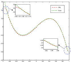
(a) $h=1/50$

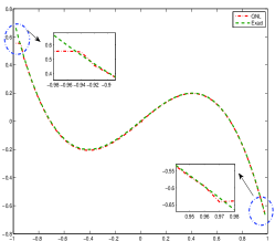
(b) $h=1/100$

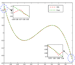
(c) $h=1/200$

Figure 2. Plots of displacement gradients (strains) for the quasinonlocal diffusion with $\delta_{1}=6h$ and $\delta_{2}=2h$ versus the local limiting diffusion at $T=1$ with various $h$. The sizes of boundary layers are of $O(2\delta_{1})$ and $O(2\delta_{2})$ on both sides, respectively.

To further study the origin of the loss of convergence order, we compute the errors of quasinonlocal solution and local limiting solution (25) measured in the energy norm within the interior of $\Omega$, that is, the errors are only measured within $[-1/2,\;1/2]$ that contains the interface $x_{0}=0$:

$$\text{Int energy err}:=\max\limits_{0\leq t\leq T}\|\nabla u(x,t)-\nabla u_{\text{exact,local}}(x,t)\|_{L^{2}([-1/2,\;1/2])}.$$ (27)

This time, we clearly observe the first order convergence rate in Table 3, further confirming that the loss of convergence is from boundary layer. In fact, this is a known problem for numerically imposing volumetric boundary condition (see e.g., [37]), which we will not go into further details here.

$h$	Int energy err of Case A	Order	Int energy err of Case B	Order
$1/50$	$2.920e$-$2$	$-$	$1.779$-$2$	$-$
$1/100$	$1.383e$-$2$	$1.07$	$8.629e$-$3$	$1.04$
$1/200$	$6.716e$-$3$	$1.04$	$4.247e$-$3$	$1.02$
$1/400$	$3.063e$-$3$	$1.13$	$2.106e$-$3$	$1.01$

Table 3. Interior errors of quasinonlocal solution and local limiting solution (25) measured in energy norm (27). Case A: $\delta_{1}=6h$ and $\delta_{2}=2h$; Case B: $\delta_{1}=4h$ and $\delta_{2}=2h$. The final simulation time is $T=1$.

Next we fix $h=1/200$, $\delta_{1}=5h$, $\delta_{2}=h$, and consider initial datum which has a singularity at $x^{*}=-0.45+h/2$.

$$u(x,0)=\frac{\sin(\pi x)}{x-x^{*}},\quad f(x)=0.$$

The solution $u(x,t)$ is plotted for $T=1/4$ in Figure 3. We can see that the quasinonlocal diffusion matches the fully nonlocal model, whereas the result of the fully local diffusion is distinguishable from that of fully nonlocal model.

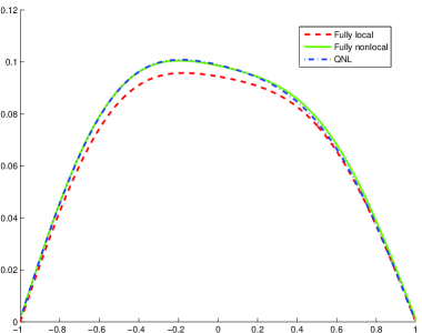
Figure 3. The solution $u(x,t)$ is plotted for $T=1/4$.

6. Conclusion

We have proposed a new self-adjoint, consistent and stable coupling strategy for nonlocal diffusion problems in one dimensional space, which couples two nonlocal operators associated with different horizon parameters $\delta_{1}$ and $\delta_{2}$ with $M:=\frac{\delta_{1}}{\delta_{2}}$ being an integer. This new coupling model is proved to be self-adjoint and patch-test consistent. In addition, the quasinonlocal diffusion is also stable (coercive) with respect to the energy norm induced by the nonlocal diffusion kernels as well as the $L^{2}$ norm, and it satisfies the maximum principle.

We also consider a first order finite difference approximation to discretize the continuous coupling model. This numerical approximation preserves the self-adjointness, consistency, coercivity and the maximum principle. The numerical scheme is validated through several examples.

Also, as for future works, another immediate direction is extending the coupling scheme to higher dimensions; as already mentioned, since the nonlocal diffusion model only involves pairwise interactions in the form of $u(y)-u(x)$, the extension should not pose serious difficulties. Better numerical approximation to the continuous quasinonlocal diffusion operator is also another interesting direction to pursue. Another interesting topic is to couple the nonlocal diffusion operator directly with local diffusion (Laplace) operator in the framework of the quasinonlocal coupling (see [1, 17, 8, 30, 12] for some recent works that couple the local and nonlocal diffusions together).

Appendix A Derivation of $\mathcal{L}^{\mathsf{qnl}}$

We give the deviation of the coupled diffusion operator $\mathcal{L}^{{\mathsf{qnl}}}$ (11), stated as the following Proposition. The calculation is straightforward but somewhat tedious.

Proposition A.1.

The coupled quasinonlocal energy functional $E^{{\mathsf{tot}},{\mathsf{qnl}}}$ induces the quasinonlocal diffusion operator $\mathcal{L}^{\mathsf{qnl}}$ defined in (11).

Proof.

The first variation of $E^{{\mathsf{tot}},{\mathsf{qnl}}}$ with test function $\forall v\in S_{\mathsf{qnl}}$ is

$$\langle \partial E^{{\mathsf{tot}},{\mathsf{qnl}}}(u),v\rangle$$

$$= \frac{1}{2}\int_{x,y\in\mathbb{R},x\leq 0\text{ or }y\leq 0}\gamma_{\delta_{1}}(\lvert y-x\rvert)dxdy\left(u(y)-u(x)\right)\left(v(y)-v(x)\right)$$

$$+\frac{1}{2}\int_{x,y\in\mathbb{R},x>0\text{ and }y>0}dxdy\Big{[}\gamma_{\delta_{1}}(\lvert y-x\rvert)$$

$$\qquad\cdot\frac{1}{M}\sum_{j=0}^{M-1}\left(u(x+\frac{j+1}{M}(y-x))-u(x+\frac{j}{M}(y-x))\right)$$

$$\qquad\qquad\qquad\left(v(x+\frac{j+1}{M}(y-x))-v(x+\frac{j}{M}(y-x))\right)M^{2}\Big{]}=:T_{1}+T_{2}.$$

Because of the symmetry in the $T_{1}$ integral in $x$ and $y$, we can convert $T_{1}$ to

$$\begin{split}T_{1}=&\frac{1}{2}\int_{x,y\in\mathbb{R},x\leq 0\text{ or }y\leq 0}\gamma_{\delta_{1}}(\lvert y-x\rvert)dxdy\left(u(y)-u(x)\right)\left(v(y)-v(x)\right)\\ =&\int_{x,y\in\mathbb{R},x\leq 0\text{ or }y\leq 0}\gamma_{\delta_{1}}(\lvert y-x\rvert)dxdy\left(u(x)-u(y)\right)\cdot v(x).\end{split}$$ (28)

We now focus on $T_{2}$.

$$T_{2}= \frac{1}{2}\sum_{j=0}^{M-1}\int_{x,y\in\mathbb{R},x>0\text{ and }y>0}dxdy\Big{[}M\gamma_{\delta_{1}}(\lvert y-x\rvert)$$ (29)

$$\qquad\cdot\left(u(x+\frac{j+1}{M}(y-x))-u(x+\frac{j}{M}(y-x))\right)$$

$$\qquad\qquad\left(v(x+\frac{j+1}{M}(y-x))-v(x+\frac{j}{M}(y-x))\right)\Big{]}$$

$$= \frac{1}{2}\sum_{j=0}^{M-1}\int_{x,y\in\mathbb{R},x>0\text{ and }y>0}dxdy\Big{[}\frac{1}{M^{2}}\gamma_{\delta_{2}}\left(\frac{\lvert y-x\rvert}{M}\right)$$

$$\qquad\cdot\left(u(x+\frac{j+1}{M}(y-x))-u(x+\frac{j}{M}(y-x))\right)$$

$$\qquad\qquad\quad\left(v(x+\frac{j+1}{M}(y-x))-v(x+\frac{j}{M}(y-x))\right)\Big{]}$$

$$= \frac{1}{2}\sum_{j=0}^{M-1}\int_{x,y\in\mathbb{R},x>0\text{ and }y>0}dxdy\Big{[}\frac{1}{M^{2}}\gamma_{\delta_{2}}\left(\frac{\lvert y-x\rvert}{M}\right)$$

$$\qquad\qquad\cdot\left(u(x+\frac{j+1}{M}(y-x))-u(x+\frac{j}{M}(y-x))\right)v\left(x+\frac{j+1}{M}(y-x)\right)\Big{]}$$

$$-\frac{1}{2}\sum_{j=0}^{M-1}\int_{x,y\in\mathbb{R},x>0\text{ and }y>0}dxdy\Big{[}\frac{1}{M^{2}}\gamma_{\delta_{2}}\left(\frac{\lvert y-x\rvert}{M}\right)$$

$$\qquad\qquad\quad\cdot\left(u(x+\frac{j+1}{M}(y-x))-u(x+\frac{j}{M}(y-x))\right)v\left(x+\frac{j}{M}(y-x)\right)\Big{]}.$$

Let $k:=(M-1)-j=M-(j+1)$ in the second summation term of (29), we get

$$T_{2}=\frac{1}{2}\sum_{j=0}^{M-1}\int_{x,y\in\mathbb{R},x>0\text{ and }y>0}dxdy\Big{[}\frac{1}{M^{2}}\gamma_{\delta_{2}}\left(\frac{\lvert y-x\rvert}{M}\right)$$ (30)

$$\qquad\cdot\left(u(x+\frac{j+1}{M}(y-x))-u(x+\frac{j}{M}(y-x))\right)v\left(x+\frac{j+1}{M}(y-x)\right)\Big{]}$$

$$-\frac{1}{2}\sum_{k=0}^{M-1}\int_{x,y\in\mathbb{R},x>0\text{ and }y>0}dxdy\Big{[}\frac{1}{M^{2}}\gamma_{\delta_{2}}\left(\frac{\lvert y-x\rvert}{M}\right)$$

$$\cdot\left(u(\frac{k}{M}x+(1-\frac{k}{M})y)-u(\frac{k+1}{M}x+(1-\frac{k+1}{M})y)\right)v\left(\frac{k+1}{M}x+(1-\frac{k+1}{M})y\right)\Big{]}$$

$$=\frac{1}{2}\sum_{j=0}^{M-1}\int_{x,y\in\mathbb{R},x>0\text{ and }y>0}dxdy\Big{[}\frac{1}{M^{2}}\gamma_{\delta_{2}}\left(\frac{\lvert y-x\rvert}{M}\right)$$

$$\qquad\cdot\left(u(x+\frac{j+1}{M}(y-x))-u(x+\frac{j}{M}(y-x))\right)v\left(x+\frac{j+1}{M}(y-x)\right)\Big{]}$$

$$+\frac{1}{2}\sum_{k=0}^{M-1}\int_{x,y\in\mathbb{R},x>0\text{ and }y>0}dxdy\Big{[}\frac{1}{M^{2}}\gamma_{\delta_{2}}\left(\frac{\lvert y-x\rvert}{M}\right)$$

$$\qquad\quad\cdot\left(u(y+\frac{k+1}{M}(x-y))-u(y+\frac{k}{M}(x-y))\right)v\left(y+\frac{k+1}{M}(x-y)\right)\Big{]}.$$

Changing the notation order of $x$ and $y$ in the second integral of (30), we have

$$T_{2}= \sum_{j=0}^{M-1}\int_{x,y\in\mathbb{R},x>0\text{ and }y>0}dxdy\Big{[}\frac{1}{M^{2}}\gamma_{\delta_{2}}\left(\frac{\lvert y-x\rvert}{M}\right)$$

$$\qquad\cdot\left(u(x+\frac{j+1}{M}(y-x))-u(x+\frac{j}{M}(y-x))\right)v\left(x+\frac{j+1}{M}(y-x)\right)\Big{]}.$$ (31)

Now let $z:=x+\frac{j+1}{M}(y-x)$ to replace $y$, then the integration interval for $z$ becomes

$$z=\left(1-\frac{j+1}{M}\right)x+\frac{j+1}{M}y>\left(1-\frac{j+1}{M}\right)x.$$

(A) thus becomes

$$T_{2}= \sum_{j=0}^{M-1}\int_{x>0\text{ and }z>(1-\frac{j+1}{M})x}\Big{[}\frac{1}{M(j+1)}$$ (32)

$$\qquad\gamma_{\delta_{2}}\left(\frac{\lvert z-x\rvert}{j+1}\right)\cdot\left(u(z)-u(z+\frac{1}{j+1}(x-z))\right)v\left(z\right)\Big{]}~{}dxdz$$

$$= \frac{1}{M}\sum_{j=0}^{M-1}\int_{z>0\text{ and }0<x<\frac{M}{M-(j+1)}z}dxdz\Big{[}\frac{1}{(j+1)}\gamma_{\delta_{2}}\left(\frac{\lvert z-x\rvert}{j+1}\right)$$

$$\qquad\qquad\qquad\qquad\qquad\qquad\cdot\left(u(z)-u(z+\frac{1}{j+1}(x-z))\right)v\left(z\right)\Big{]},$$

where $\frac{M}{M-(j+1)}z$ is formally regarded as $+\infty$ when $j=M-1$.

Now let $w=z+\frac{1}{j+1}(x-z)=\frac{j}{j+1}z+\frac{1}{j+1}x$ to replace x, thus the integration interval for $w$ is

$$z-\frac{1}{j+1}z<w<z+\frac{1}{M-(j+1)}z,$$

and we have $T_{2}$:

$$T_{2}= \frac{1}{M}\sum_{j=0}^{M-1}\int_{z>0\text{ and }z-\frac{1}{j+1}z<w<z+\frac{1}{M-(j+1)}z}\Big{[}\gamma_{\delta_{2}}\left(\lvert w-z\rvert\right)\cdot\left(u(z)-u(w)\right)v\left(z\right)\Big{]}~{}dwdz$$

$$= \frac{1}{M}\sum_{j=1}^{M}\int_{z>0\text{ and }z-\frac{1}{j}z<w<z+\frac{1}{M-(j)}z}\Big{[}\gamma_{\delta_{2}}\left(\lvert w-z\rvert\right)\cdot\left(u(z)-u(w)\right)v\left(z\right)\Big{]}~{}dwdz$$

$$= \frac{1}{M}\sum_{j=1}^{M-1}\int_{z>0\text{ and }z-\frac{1}{j}z<w<z+\frac{1}{j}z}\Big{[}\gamma_{\delta_{2}}\left(\lvert w-z\rvert\right)\cdot\left(u(z)-u(w)\right)v\left(z\right)\Big{]}~{}dwdz$$

$$\quad+\frac{1}{M}\int_{z>0\text{ and }z-\frac{1}{M}z<w<\infty}\Big{[}\gamma_{\delta_{2}}\left(\lvert w-z\rvert\right)\cdot\left(u(z)-u(w)\right)v\left(z\right)\Big{]}~{}dwdz.$$ (33)

Now, we combine $T_{1}$ (28) and $T_{2}$ (A) together, we have

$$\langle \partial E^{{\mathsf{tot}},{\mathsf{qnl}}}(u),v\rangle$$

$$=\int_{x,y\in\mathbb{R},x\leq 0\text{ or }y\leq 0}\gamma_{\delta_{1}}(\lvert y-x\rvert)\left(u(x)-u(y)\right)\cdot v(x)dxdy$$

$$\quad+\frac{1}{M}\sum_{j=1}^{M-1}\int_{z>0\text{ and }z-\frac{1}{j}z<w<z+\frac{1}{j}z}\Big{[}\gamma_{\delta_{2}}\left(\lvert w-z\rvert\right)\cdot\left(u(z)-u(w)\right)v\left(z\right)\Big{]}~{}dwdz$$

$$\qquad+\frac{1}{M}\int_{z>0\text{ and }z-\frac{1}{M}z<w<\infty}\Big{[}\gamma_{\delta_{2}}\left(\lvert w-z\rvert\right)\cdot\left(u(z)-u(w)\right)v\left(z\right)\Big{]}~{}dwdz$$

$$=\int_{x,y\in\mathbb{R},x\leq 0\text{ or }y\leq 0}\gamma_{\delta_{1}}(\lvert y-x\rvert)\left(u(x)-u(y)\right)\cdot v(x)dxdy$$

$$\quad+\frac{1}{M}\sum_{j=1}^{M-1}\int_{x>0\text{ and }x-\frac{1}{j}x<y<x+\frac{1}{j}x}\Big{[}\gamma_{\delta_{2}}\left(\lvert y-x\rvert\right)\cdot\left(u(x)-u(y)\right)v\left(x\right)\Big{]}~{}dxdy$$

$$\qquad+\frac{1}{M}\int_{x>0\text{ and }x-\frac{1}{M}x<y<\infty}\Big{[}\gamma_{\delta_{2}}\left(\lvert y-x\rvert\right)\cdot\left(u(x)-u(y)\right)v\left(x\right)\Big{]}~{}dxdy,$$ (34)

where we just replaces the notations $z$ by $x$ and $w$ by $y$.

The corresponding diffusion operator $\mathcal{L}^{\mathsf{qnl}}$ is equal to negative of the first order variation of $E^{{\mathsf{tot}},{\mathsf{qnl}}}(u)$, which can be discussed in three cases below:

1. Case I: $x\leq 0$:

   $$\mathcal{L}^{\mathsf{qnl}}u(x)=\int_{y\in\mathbb{R}}\gamma_{\delta_{1}}(\lvert y-x\rvert)\left(u(x)-u(y)\right)dy.$$

2. Case II: $0<x<\delta_{1}$:

   $$\begin{split}\mathcal{L}^{\mathsf{qnl}}u(x)=&\int_{x-\delta_{1}<y<0}\gamma_{\delta_{1}}(\lvert y-x\rvert)\left(u(x)-u(y)\right)dy\\ &\quad+\frac{1}{M}\sum_{j=1}^{M-1}\int_{x-\frac{1}{j}x<y<x+\frac{1}{j}x}\gamma_{\delta_{2}}\left(\lvert y-x\rvert\right)\cdot\left(u(x)-u(y)\right)dy\\ &\qquad\qquad+\frac{1}{M}\int_{x-\frac{1}{M}x<y<\infty}\gamma_{\delta_{2}}\left(\lvert y-x\rvert\right)\cdot\left(u(x)-u(y)\right)dy.\end{split}$$

3. Case III: $x\geq\delta_{1}$:

   $$\begin{split}\mathcal{L}^{\mathsf{qnl}}u(x)=&\frac{1}{M}\sum_{j=1}^{M-1}\int_{x-\frac{1}{j}x<y<x+\frac{1}{j}x}\gamma_{\delta_{2}}\left(\lvert y-x\rvert\right)\cdot\left(u(x)-u(y)\right)dy\\ &\qquad\qquad+\frac{1}{M}\int_{x-\frac{1}{M}x<y<\infty}\gamma_{\delta_{2}}\left(\lvert y-x\rvert\right)\cdot\left(u(x)-u(y)\right)dy.\end{split}$$

   Notice that $x\geq\delta_{1}$, thus

   $$x-\frac{1}{j}x<x-\frac{1}{M}x<x-\frac{1}{M}\delta_{1}=x-\delta_{2},$$

   and

   $$x+\frac{1}{j}x>x+\frac{1}{M}x>x+\frac{1}{M}\delta_{1}=x+\delta_{2}.$$

   Because outside the support, the diffusion kernel is zero, therefore, we have

   $$\begin{split}\mathcal{L}^{\mathsf{qnl}}u(x)=&\frac{1}{M}\sum_{j=1}^{M-1}\int_{x-\delta_{2}<y<x+\delta_{2}}\gamma_{\delta_{2}}\left(\lvert y-x\rvert\right)\cdot\left(u(x)-u(y)\right)dy\\ &\qquad\qquad+\frac{1}{M}\int_{x-\delta_{2}<y<\infty}\gamma_{\delta_{2}}\left(\lvert y-x\rvert\right)\cdot\left(u(x)-u(y)\right)dy\\ =&\int_{x-\delta_{2}<y<x+\delta_{2}}\gamma_{\delta_{2}}\left(\lvert y-x\rvert\right)\cdot\left(u(x)-u(y)\right)dy\\ =&\int_{y\in\mathbb{R}}\gamma_{\delta_{2}}\left(\lvert y-x\rvert\right)\cdot\left(u(x)-u(y)\right)dy.\end{split}$$

Hence, we get (11). ∎

References

- [1] E. Askari, F. Bobaru, R. B. Lehoucq, M. L. Parks, S. A. Silling, and O. Weckner. Peridynamics for multiscale materials modeling. Journal of Physics: Conference Series, 125(1), 2008.
- [2] P. Bates and A. Chmaj. An integrodifferential model for phase transitions: Stationary solutions in higher space dimensions. Journal of Statistical Physics, 95:1119–1139, 1999.
- [3] T. Belytschko and T. Black. Elastic crack growth in finite elements with minimal remeshing. International Journal for Numerical Methods in Engineering, 45:601–620, 1999.
- [4] F. Bobaru and M. Duangpanya. The peridynamic formulation for transient heat conduction. International Journal of Heat and Mass Transfer, 53:4047–4059, 2010.
- [5] L. Caffarelli, C. H. Chan, and A. Vasseur. Regularity theory for parabolic nonlinear integral operators. J. Amer. Math. Soc., 24:849–869, 2011.
- [6] E. Chasseigne, M. Chaves, and J. D. Rossi. Asymptotic behavior for nonlocal diffusion equations. Journal de Mathématiques Pures et Appliquées, 86:271–291, 2006.
- [7] M. D’Elia and M. Gunzburger. Optimal distributied control of nonlocal steady diffusion problems. SIAM Journal on Control and Optimization, 52:243–273, 2014.
- [8] M. D’Elia, M. Perego, P. Bochev, and D. Littlewood. A coupling strategy for nonlocal and local diffusion models with mixed volume constraints and boundary conditions. Computers and Mathematics with applications, 71(11):2218–2230, 2015.
- [9] Q. Du, M. Gunzburger, R. Lehoucq, and K. Zhou. Analysis and approximation of nonlocal diffusion problems with volume constraints. SIAM Review, 56:676–696, 2012.
- [10] Q. Du, M. Gunzburger, R. Lehoucq, and K. Zhou. A nonlocal vector calculus, nonlocal volume-constrained problems, and nonlocal balance laws. Mathematical Models and Methods in Applied Sciences, 23:493–540, 2013.
- [11] Q. Du, L. Ju, L. Tian, and K. Zhou. A posteriori error analysis of finite element method for linear nonlocal diffusion and peridynamic models. Mathematics of Computation, 82:1889–1922, 2013.
- [12] Q. Du and X. Tian. Seamless coupling of nonlocal and local models. preprint.
- [13] W. E, J. Lu, and J. Z. Yang. Uniform accuracy of the quasicontinuum method. Phys. Rev. B, 74(21):214115, 2006.
- [14] P. Fife. Some nonclassical trends in parabolic and parabolic-like evolutions. In Trends in Nonlinear Analysis, pages 153–191. Springer, 2003.
- [15] Y. D. Ha and F. Bobaru. Studies of dynamic crack propagation and crack branching with peridynamics. International Journal of Fracture, 162:229–244, 2010.
- [16] Y. D. Ha and F. Bobaru. Characteristics of dynamic brittle fracture captured with peridynamics. Engineering Fracture Mechanics, 78:1156–1168, 2011.
- [17] F. Han and G. Lubineau. Coupling of nonlocal and local continuum models by the arlequin approach. International Journal for Numerical Methods in Engineering, 89(6):671–685, 2012.
- [18] A. Hillerborg, M. Modeer, and P. Petersson. Analysis of crack formation and crack growth by means of fracture mechanics and finite elements. Cement and Concrete Research, 6:773–781, 1976.
- [19] S. Kohlhoff and S. Schmauder. A new method for coupled elastic-atomistic modelling. Atomistic Simulation of Materials: Beyond Pair Potentials, pages 411–418, 1989.
- [20] D. Kriventsov. Regularity for a local-nonlocal transmission problem, 2014. preprint, arXiv:1404.1363.
- [21] X. H. Li and M. Luskin. A generalized quasinonlocal atomistic-to-continuum coupling method with finite-range interaction. IMA Journal of Numerical Analysis, 32:373–393, 2011.
- [22] R. Lipton. Cohesive dynamics and brittle fracture. Journal of Elasticity, 124:143–191, 2016.
- [23] G. Lubineau, Y. Azdoud, F. Han, C. Rey, and A. Askari. A morphing strategy to couple nonlocal to local continuum mechanics. Journal of the Mechanics and Physics of Solids, 60(6):1088–1102, 2012.
- [24] M. Luskin and C. Ortner. Atomistic-to-continuum-coupling. Acta Numerica, 22(4):397–508, 2013.
- [25] R. Miller and E. Tadmor. A unified framework and performance benchmark of fourteen multiscale atomistic/continuum coupling methods. Modelling and Simulation in Materials Science and Engineering, 17(5):053001, 2009.
- [26] P. Ming and J. Z. Yang. Analysis of a one-dimensional nonlocal quasicontinuum method. Multiscale Modeling and Simulation, 7:1838–1875, 2009.
- [27] C. Ortner and L. Zhang. Energy-based atomistic-to-continuum coupling without ghost forces. Computer Methods in Applied Mechanics and Engineering, 279:29–45, 2014.
- [28] S. Prudhomme, H. Ben Dhia, P. T. Bauman, N. Elkhodja, and J. T. Oden. Computational analysis of modeling error for the coupling of particle and continuum models by the Arlequin method. Computer Methods in Applied Mechanics and Engineering, 197(41-42):3399–3409, 2008.
- [29] P. Seleson, S. Beneddine, and S. Prudhomme. A force based coupling scheme for peridynamics and classical elasticity. Computational Materials Science, 66:34–49, 2013.
- [30] P. Seleson, Y. D. Ha, and S. Beneddine. Concurrent coupling of bond based peridynamics and the navier equation of classical elasticity by blending. Journal for Multiscale Computational Engineering, 13:91–113, 2015.
- [31] A. V. Shapeev. Consistent energy-based atomistic/continuum coupling for two-body potentials in one and two dimensions. Multiscale Modeling and Simulation, 9(3):905–932, 2012.
- [32] T. Shimokawa, J. J. Mortensen, J. Schiotz, and K. W. Jacobsen. Matching conditions in the quasicontinuum method: Removal of the error introduced at the interface between the coarse-grained and fully atomistic region. Phys. Rev. B, 69(21):214104, 2004.
- [33] S. Silling. Reformulation of elasticity theory for discontinuities and long-range forces. Journal of the Mechanics and Physics of Solids, 48:175–209, 2000.
- [34] S. Silling and R. B. Lehoucq. Peridynamic theory of solid mechanics. Advances in Applied Mechanics, 44:73–168, 2010.
- [35] S. Silling, D. J. Littlewood, and P. Seleson. Variable horizon in a peridynamic medium. Journal of Mechancis of Materials and Structures, 10(5):591–612, 2015.
- [36] X. Tian and Q. Du. Trace theorems for some nonlocal function spaces with heterogeneous localization. submitted to SIAM Journal on Mathematical Analysis.
- [37] X. Tian and Q. Du. Analysis and comparison of different approximations to nonlocal diffusion and linear peridynamic equations. SIAM Journal on Numerical Analysis, 51:3458–3482, 2013.
- [38] X. Tian and Q. Du. Asymptotically compatible schemes and applications to robust discretization of nonlocal models. SIAM Journal on Numerical Analysis, 52:1641–1665, 2014.
- [39] X. Tian and Q. Du. A class of high order nonlocal operators. Archive for Rational Mechanics and Analysis, 222:1521–1553, 2016.
- [40] H. Yao and H. Gao. Multi-scale cohesive laws in hierarchical materials. International Journal of Solids and Structures, 44:8177–8193, 2007.