Multicritical behavior of the two-dimensional transverse Ising metamagnet in a longitudinal magnetic field

Abstract

ABSTRACT

Magnetic phenomena of the superantiferromagnetic Ising model in both uniform longitudinal ($H$) and transverse ($\Omega$) magnetic fields are studied by employing a mean-field variational approach based on Peierls-Bogoliubov inequality for the free energy. A single-spin cluster is used to get the approximate thermodynamic properties of the model. The phase diagrams in the magnetic fields and temperature ($T$) planes, namely, $H-T$ and $\Omega-T$, are analyzed on an anisotropic square lattice for some values of the ratio $\alpha=J_{y}/J_{x}$, where $J_{x}$ and $J_{y}$ are the exchange interactions along the $x$ and $y$ directions, respectively. Depending on the range of the Hamiltonian parameters, one has only second-order transition lines, only first-order transition lines, or first- and second-order transition lines with the presence of tricritical points. The corresponding phase diagrams show no reentrant behavior along the first-order transition lines at low temperatures. These results are different from those obtained by using Effective Field Theory with the same cluster size.

PACS numbers: 64.60.Ak; 64.60.Fr; 68.35.Rh

I Introduction

Theoretical metamagnetic models are systems that have both antiferromagnetic and ferromagnetic coupling interactions. At zero external field meijer1978 ; kincaid1975 , they undergo a second-order phase transition at the Néel temperature $T_{N}$. Besides the usual nearest-neighbor staggered arrangements of the spins, the ordered phase can be, for instance, ferromagnetic planes ordered antiferromagnetically to each other, or even ferromagnetic chains ordered antiferromagnetically, where the latter phase is usually called a superantiferromagnetic phase. At non-zero field, applyied longitudinally to the direction of the magnetization, the Néel transition temperature decreases as the magnitude of the external field increases and the line of second-order transition comes to an end at a finite temperature. Beyond this point, the transition is first order and ends up, at zero temperature, at a finite field $H_{c}$. This phenomenon has been previously well described by Landau landau1937 and by Griffiths griffits1970 , where one has the presence of a tricritical point (the point joining first- and second-order transition lines).

On the other hand, through the years, experimental realizations of magnetic materials exhibiting the above characteristics have been studied. For example, Chernyi and co-workers chernyi have considered the kinetics of a magnetization process in quasi-one-dimensional Ising superantiferromagnet named as trimethylammonium cobalt chloride [(CH₃)₃NH]CoCl${}_{3}\cdot$2H₂O, denoted by CoTAC, belonging to a wider series of organometallic compounds with general chemical formula [(CH₃)₃MX₃]CoCl${}_{3}\cdot$2H₂O with M=Mn, Co, Ni, Fe, and X=Br or Cl. However, one of the first studies known in the literature on the effects of a longitudinal magnetic field in superantiferromagnetic systems has been done on the (C₂H₅NH₃)₂CuCl₄ compound dejongh .

It is worth mentioning that superfluid mixtures of the two helium isotopes ³He and ⁴He, and a class of anisotropic metamagnets such as FeCl₂, FeBr₂ and Ni(NO₃)${}_{2}\cdot 2$H₂O, although microscopically different at first sight, show in their thermodynamic behavior a striking similarity in that they exhibit a phase diagram in which a line of $\lambda-$type transition points (second-order transition line) ends up at a tricritical point (see, for instance, reference kincaid1975 ).

Based on these real experimentations, we will treat herein a quantum version of a metamagnet conveying not only the basic features of the relevant classical interactions above discussed, which leads to a tricritical behavior similar to the well known classical Blume-Capel bc and BEG models beg, but also the inclusion of quantum fluctuations due to a transverse field, which will be in fact important in the low temperature regime. Moreover, there has been, in recent years, an extensive literature on competitive interaction models that present a superantiferromagnetic (SAF) ordering, where, for instance, ferromagnetic chains are coupled in an antiferromagnetic way in two dimensions. According to these lines, the system to be treated herein corresponds to a two-dimensional spin-$1/2$ Ising model with different exchange interactions along the two lattice directions, in the presence of transverse and longitudinal magnetic fields. Additional motivations to study the Ising model is because it can be used to describe the critical behavior of a broader class of materials, including easy-axis magnets, binary alloys, simple liquids and their mixtures, polymer solutions, subnuclear matter, etc. ising1; ising2; ising3.

In the present case, the corresponding model can be described by the following Hamiltonian

$$\mathcal{H}=-J_{x}\sum_{{\left<i,j\right>}_{x}}\sigma_{i}^{z}\sigma_{j}^{z}+J_{y}\sum_{{\left<i,j\right>}_{y}}\sigma_{i}^{z}\sigma_{j}^{z}-H\sum_{i=1}^{N}\sigma_{i}^{z}-\Omega\sum_{i=1}^{N}\sigma_{i}^{x},$$ (1)

where $\sigma_{i}^{\mu}$ is the $\mu(=x,y)$ Pauli spin-$1/2$ operator component at site $i$ on a square lattice of $N$ sites, $J_{x}>0(J_{y}>0)$ is the exchange coupling along the $x(y)$ axis, the first and second sum are over nearest-neighbors along the $x$ and $y$ axis, respectively, $H$ is the longitudinal magnetic field, and $\Omega$ is the transverse magnetic field. The corresponding ordered state is composed by a superantiferromagnetic phase, and is characterized by a parallel spin orientation in the $x$ direction, and an antiparallel spin orientation in the $y$ direction, therefore exhibiting a kind of Néel order between two sublattices of linear chains that can be denoted by $A$ and $B$.

The classical version of model (1), i.e. $\Omega=0$, on anisotropic square lattices has been investigated by using a modified mean-field theory, in which the intrachain interaction is treated exactly and the interactions between chains are taken into account in a mean-field way (linear chain approximation - LCA) stout; hone; sato; lca; pla2. Several other approaches, such as usual mean-field approximation (MFA) garrett; ziman; rottman1990, effective-field theory (EFT) minos2006; zukovic; sousa2013, mean-field renormalization group (MFRG) slotte, effective-field renormalization group (EFRG) neto2004, Monte Carlo simulations (MC) viana2009; landau; landau1976; ferrenberg; otavio, and high-temperature series expansion (SE) bienenstock have also been applied to this classical model. Although these approaches agree with the overall phase diagram in two dimensions, LCA lca and EFT minos2006 approaches produce a reentrant behavior in the first-order transition line. The same reentrant behavior is obtained for the three-dimensional model by the EFT with four spins sousa2013.

On the other hand, the quantum version of the model, given by the Hamiltonian (1), has not been ubiquitously treated in the literature as its classical counterpart. Nevertheless, phase diagrams and some thermodynamic properties have been obtained by using the EFT deni1; deni2, and a pair approximation for the free energy (the latter case only for $J_{y}<0$ pla). It has been noted that only second-order phase transitions are present in the computed phase diagrams.

In the present paper, using the MFA based on a variational method for the free- energy, we investigate the phase diagram behavior of the spin-$1/2$ Ising superantiferromagnet in the presence of both longitudinal and transverse external fields. We would like to seek out not only the effect of the quantum fluctuations in the model but also the presence or not of the tricritical points and first-order transitions, since the EFT has only given a second-order character.

The remaining of the paper is organized as follows. In the next section we outline the formalism and its application to the transverse Ising superantiferromagnet in the presence of a longitudinal magnetic field; in Sec. III we discuss the results and present some final comments.

II Formalism

We will treat model (1) by the mean-field approximation (MFA) using a variational method based on Peierls-Bogoliubov inequality, which can be formally written as

$$F\left(\mathcal{H}\right)\leq F_{0}\left(\mathcal{H}_{0}\right)+\left\langle\mathcal{H}-\mathcal{H}_{0}\right\rangle_{0}\equiv\Phi(\gamma),$$ (2)

where $F$ and $F_{0}$ are free energies associated with two systems defined by the Hamiltonians $\mathcal{H}$ and $\mathcal{H}_{0}(\gamma)$, respectively, the thermal average $<...>_{0}$ should be taken in relation to the canonical distribution associated with the trial Hamiltonian $\mathcal{H}_{0}(\gamma)$, with $\gamma$ standing for the variational parameters. The approximated free energy $F$ is then given by the minimum of $\Phi(\gamma)$ with respect to $\gamma$, i.e. $F\equiv\Phi_{min}(\gamma)$.

The trial Hamiltonian $\mathcal{H}_{0}$ is chosen as free spins, distributed in two different sublattices $A$ and $B$. Each sublattice consists of ferromagnetic linear chains coupled antiferromagnetically with two neighboring chains. We then have

$$\mathcal{H}_{0}=-\gamma_{A}\sum_{i\subset A}\sigma_{i}^{z}-\Omega\sum_{i\subset A}\sigma_{i}^{x}-\gamma_{B}\sum_{i\subset B}\sigma_{i}^{z}-\Omega\sum_{i\subset B}\sigma_{i}^{x},$$ (3)

where $\gamma_{A}$ and $\gamma_{B}$ are two variational parameters.

It is not difficult to compute the right hand side of Eq. (2) and, after minimizing $\Phi(\gamma)$, the variational parameters $\gamma_{A}$ and $\gamma_{B}$ can be written as a function of the sublattice magnetizations $m_{A}$ and $m_{B}$. The approximated mean-field Helmholtz free energy per spin, $f=\frac{\Phi}{N}$, can thus be written as

$$f = \frac{t}{2}\ln\left\{4\cosh\frac{1}{t}\sqrt{\left(h+2m_{A}-2\alpha m_{B}\right)^{2}+\delta^{2}}\cosh\frac{1}{t}\sqrt{\left(h+2m_{B}-2\alpha m_{A}\right)^{2}+\delta^{2}}\right\}$$ (5)

$$-\alpha m_{A}m_{B}+\frac{1}{2}\left(m_{A}^{2}+m_{B}^{2}\right),$$

with the corresponding sublattice magnetizations $m_{A}$ and $m_{B}$ given by

$$m_{A}=\frac{h+2\left(m_{A}-\alpha m_{B}\right)}{\sqrt{\left(h+2m_{A}-2\alpha m_{B}\right)^{2}+\delta^{2}}}\tanh\frac{1}{t}\sqrt{\left(h+2m_{A}-2\alpha m_{B}\right)^{2}+\delta^{2}},$$ (6)

and

$$m_{B}=\frac{h+2\left(m_{B}-\alpha m_{A}\right)}{\sqrt{\left(h+2m_{B}-2\alpha m_{A}\right)^{2}+\delta^{2}}}\tanh\frac{1}{t}\sqrt{\left(h+2m_{B}-2\alpha m_{A}\right)^{2}+\delta^{2}},$$ (7)

where $t=k_{B}T/J_{x}$, $h=H/J_{x}$, $\delta=\Omega/J_{x}$ and $\alpha=J_{y}/J_{x}$ is the ratio between ferromagnetic and antiferromagnetic interactions. For a given value of the set of parameters $t$, $h$, $\delta$ and $\alpha$, Eqs. (6) and (7) are numerically solved for $m_{A}$ and $m_{B}$ and, when several solutions are found, the stable phase will be the one that minimizes the free energy $f$. In this context, the equilibrium state corresponds always to the minimum value of $f$ with respect to $m_{A}$ and $m_{B}$.

For a metamagnetic system, it is more convenient to formulate the problem in terms of the total $m$ and the staggered $m_{s}$ magnetizations, which are defined as $m=(m_{A}+m_{B})/2$ and $m_{s}=(m_{A}-m_{B})/2$. Therefore, we can rewrite eqs. (5), (6) and (7) as

$$f = -\frac{t}{2}\ln 4\sum_{p=0}^{1}\left\{\cosh\frac{1}{t}\sqrt{\left[h+2\left(1-\alpha\right)m-2\left(-1\right)^{p}\left(1+\alpha\right)m_{s}\right]^{2}+\delta^{2}}\right\}$$ (8)

$$+\left(1-\alpha\right)m^{2}+\left(1+\alpha\right)m_{s},$$

$$m = \frac{1}{2}\sum_{p=0}^{1}\frac{h+2m\left(1-\alpha\right)-2m_{s}\left(1+\alpha\right)}{\sqrt{\left[h+2m\left(1-\alpha\right)-2\left(-1\right)^{p}\left(1+\alpha\right)m_{s}\right]^{2}+\delta^{2}}}$$ (9)

$$\tanh\frac{1}{t}\sqrt{\left[h+2m\left(1-\alpha\right)-2\left(-1\right)^{p}\left(1+\alpha\right)m_{s}\right]^{2}+\delta^{2}},$$

$$m_{s} = \frac{1}{2}\sum_{p=0}^{1}\left(-1\right)^{p}\frac{h+2m\left(1-\alpha\right)-2m_{s}\left(1+\alpha\right)}{\sqrt{\left[h+2m\left(1-\alpha\right)-2\left(-1\right)^{p}\left(1+\alpha\right)m_{s}\right]^{2}+\delta^{2}}}$$ (10)

$$\tanh\frac{1}{t}\sqrt{\left[h+2m\left(1-\alpha\right)-2\left(-1\right)^{p}\left(1+\alpha\right)m_{s}\right]^{2}+\delta^{2}},$$

from which one can obtain the frontiers separating the SAF and P phases (the paramagnetic phase P consists of all spins aligned with the external longitudinal field). Although the first-order transition line must be computed by numerically seeking the minimum of the free energy, the second-order transition line, as well as the location of the tricritical point, can be obtained through a Landau expansion of the free energy, given by Eq. (8), in a power series of the order parameter $m_{s}$. After a lengthy algebra the final result can be written as

$$f\left(t,h,\delta,\alpha;m_{s}\right)=\sum_{k=0}a_{2k}\left(t,h,\delta,\alpha\right)m_{s}^{2k},$$ (11)

from which we get the second-order transition lines when $a_{2}=0$ and $a_{4}>0$, and the tricritical point when $a_{2}=0$, $a_{4}=0$ and $a_{6}>0$ (see, for instance, Refs. gul; sousa2013). In present case, $a_{0}$ is not important for our purposes, so the $a_{2}$, $a_{4}$, and $a_{6}$ coefficients can be written as

$$a_{2}=\frac{4\gamma_{2}^{2}}{\lambda}\left\{\left[\frac{\beta\gamma_{1}^{2}}{\lambda}+1\right]-\frac{4\gamma_{1}^{2}}{\lambda}\left[\beta x+\frac{x}{\lambda}\right]\right\}+2(1+\alpha),$$ (12)

$$a_{4} = \frac{1}{\beta}\left(\frac{2\beta\gamma_{1}\gamma_{2}}{\lambda}\right)^{4}\left(x^{2}-1\right)-\frac{12\beta\gamma_{2}^{4}}{\lambda^{3}}\left(\lambda-x+\lambda x\right)+\frac{24\beta x^{2}\gamma_{2}^{4}}{\lambda^{6}}\left(\gamma_{1}^{4}-\lambda^{4}\right)$$

$$+\frac{48\beta^{2}\gamma_{1}^{2}\gamma_{2}^{4}}{\lambda^{3}}\left(x^{3}-x\right)-24\left(\frac{\beta\gamma_{1}\gamma_{2}}{\lambda}\right)^{4}\left[\frac{3}{\beta}\left(\frac{x}{\beta\gamma_{1}}\right)^{2}+\left(1+\frac{1}{\beta}\right)x^{4}-\left(1+\beta x^{2}\right)\frac{1}{\beta^{2}}\right]$$

$$+\frac{24}{\beta^{2}\lambda}\left(\frac{\beta\gamma_{1}\gamma_{2}}{\lambda}\right)^{4}\left[x^{3}-\frac{x}{(\gamma_{1}\gamma_{2})^{2}}-\beta x\right]+\frac{36}{\beta^{3}\gamma_{1}^{2}}\left(\frac{\beta\gamma_{1}\gamma_{2}}{\lambda}\right)^{4}\left[2\left(1-\frac{1}{\beta\lambda}\right)+\left(\frac{\gamma_{1}x}{\beta\lambda}\right)^{2}\right]$$

$$-\frac{60\beta\gamma_{1}^{4}\gamma_{2}^{4}}{\lambda^{6}}\left(1-\frac{x}{\lambda\gamma_{2}^{2}}\right),$$

$$a_{6} = (3780x)\frac{\gamma_{1}^{6}\gamma_{2}^{6}}{\lambda^{11}}-(1200x^{2})\frac{\gamma_{1}^{6}\gamma_{2}^{6}}{\lambda^{10}}+\Psi_{1}(\gamma_{1},\gamma_{2},\beta,x)\mathcal{O}\left(\frac{1}{\lambda^{9}}\right)$$

$$+\Psi_{2}(\gamma_{1},\gamma_{2},\beta,x)\mathcal{O}\left(\frac{1}{\lambda^{8}}\right)+\Psi_{3}(\gamma_{1},\gamma_{2},\beta,x)\mathcal{O}\left(\frac{1}{\lambda^{7}}\right)+\Psi_{4}(\gamma_{1},\gamma_{2},\beta,x)\mathcal{O}\left(\frac{1}{\lambda^{6}}\right)$$

$$+\Psi_{5}(\gamma_{1},\gamma_{2},\beta,x)\mathcal{O}\left(\frac{1}{\lambda^{5}}\right)+\Psi_{6}(\gamma_{1},\gamma_{2},\beta,x)\mathcal{O}\left(\frac{1}{\lambda^{4}}\right)+120(x+2x^{2})\frac{\beta^{2}\gamma_{2}^{6}}{\lambda^{3}},$$

where $\lambda^{2}=\gamma_{2}^{2}+\delta^{2}$, $\gamma_{1}=h+2(1-\alpha)m^{2}$, $\gamma_{2}=2(1+\alpha)$ and $x=\tanh(\beta\lambda)$. The functions $\Psi_{i}$, $i=2,~{}3,...,6$, are rather lengthy to be reproduced here.

III Results and Discussion

Depending on the value of the Hamiltonian parameters, the model (1) has first- or second-order phase transitions from the superantiferromagnetic phase (SAF) to the paramagnetic phase (P). For $\Omega=0$, one has the well known mean-field results for the classical model, in which the critical temperature decreases from $t_{c}=2+2\alpha$ as the longitudinal field increases and, at $T=0$ (ground-state), a first-order transition occurs at $h_{c}=2\alpha$. The tricritical point is located at $t_{t}=2.667$ and $h_{t}=1.756$ for the isotropic lattice $\alpha=1$. It would then be quite interesting to see the global effects of the quantum fluctuations, which are driven by the transverse field, on the corresponding phase diagram.

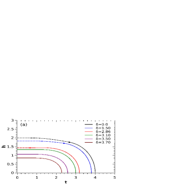
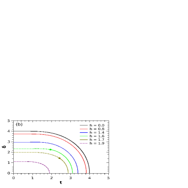
Figure 1: Phase diagrams for the isotropic square lattice ($\alpha=1.0$). (a) In the reduced temperature $t$ versus reduced longitudinal magnetic field $h$ plane, for several values of $\delta$. (b) In the reduced temperature $t$ versus the reduced transverse field $\delta$, for several values of $h$.

In Figs. 1(a) and 1(b) we have the phase diagrams in the $h-t$ (for some selected values of $\delta$) and $\delta-t$ (for some selected values of $h$) planes, in the isotropic lattice case $\alpha=1$. From Fig. 1(a) we can see that as the transverse field increases, the transition temperature decreases. This is a result of the quantum fluctuations destroying not only the superantiferromagnetic order among chains, but also the corresponding ferromagnetic order inside each chain. The first-order line and the tricritical point survive up to $\delta\simeq 2.86$ (this value, as well as the ones given below, can be numerically obtained with much more precision. However, for the sake of simplicity, we will only present them with two decimal digits). For $2.87\lesssim\delta\leq 4$ the transition is always second order, and quantum phase transitions start to develop at $T=0$, while for $\delta>4$ the system is always in the paramagnetic phase.

Fig. 1(b) presents the corresponding phase diagram in the $\delta-t$ plane for several values of $h$ and again $\alpha=1$. For $h=0$, we have the mean-field solution of the transverse Ising model, where the critical temperature goes to zero at the known value $\delta=4$. As expected, by increasing the longitudinal field the transition temperature decreases. For $0<h\lesssim 1.48$ the transition is always second order. Tricritical points and first-order transition lines, at low temperatures, appear for $1.49\lesssim h\lesssim 1.80$ (in this region, the critical quantum phase transition is suppressed). In the range $1.81\lesssim h\leq 2$, only first-order transition is observed and, for $h>2$, the system is always in the paramagnetic phase for any value of the temperature.

In Figs. 2(a) and 2(b) we have the phase diagrams for the anisotropic lattice $\alpha=0.5$. The general behavior is the same, we have only changes in the values of the corresponding Hamiltonian parameters. For instance, in the $h-t$ plane the tricritical point survives for $\delta\lesssim 2.31$, for $2.32\lesssim\delta\leq 3$ only second-order transition lines are present and for $\delta>3$ the system is always in the paramagnetic phase. In the $\delta-t$ plane one has always second-order transitions for $0<h\lesssim 0.60$, tricritical points and first-order transition lines appear for $0.61\lesssim h\lesssim 0.69$, only first-order transitions occur for $0.70\lesssim h\leq 2$, and the paramagnetic phase is always stable for $h>2$. Note here the smaller range of $h$ for having first-order and tricritical points in this plane phase diagram.

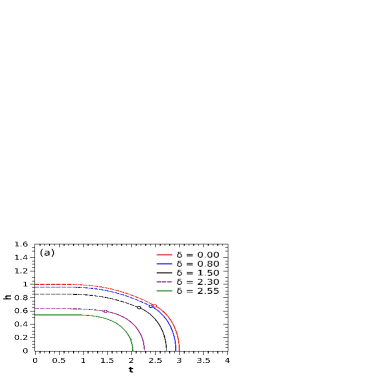
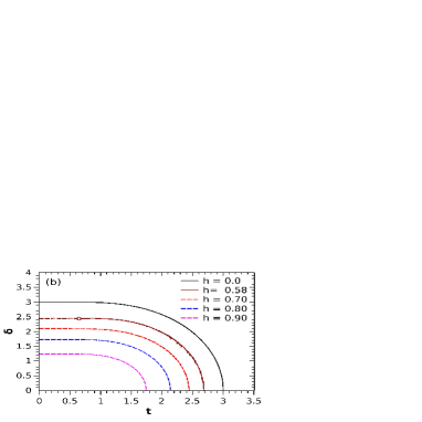
Figure 2: The same as Fig 1 for $\alpha=0.5$.

The same trend is achieved for still smaller values of $\alpha$, where a crossover from the two-dimensional behavior to the one-dimensional behavior is observed when $\alpha\rightarrow 0$. For this quasi-one-dimensional model, however, the range of the parameters in order to observe multicritical phenomena gets narrower, and it is sometimes difficult to numerically access it. Moreover, as the present one-spin mean-field approach provides a final transition temperature even in one dimension, better procedures should be very welcome to treat the present model. Nevertheless, from the present results, one can clearly see that the results are indeed different from those obtained by employing EFT deni1; deni2 and no reentrant behavior is observed in the first-order transition lines at low temperatures. The same qualitative results are expected for the model in three-dimensions, where the chains are arranged in a staggered way.

IV Conclusions

In summary, we investigated the anisotropic two-dimensional nearest-neighbor Ising model with competitive interations in an uniform longitudinal and traverse fields by using the MFA approach. We obtained the phase diagrams in the $h-T$ and $\delta-T$ planes varying the value of $\alpha$, where the critical frontier separates the SAF order with the paramagnetic disorder.

At zero temperature, the critical field is exactly obtained, so $h_{c}=2+2\alpha$. For a $\delta=0$, the model reproduces the classic result minos2006. We see that there are the same trend is achieved for still smaller values of $\alpha$, where a crossover from the two-dimensional behavior to the one-dimensional behavior is observed when $\alpha\rightarrow 0$.

We showed also that for this approach appear in the phase diagrams lines of the first order as well as tri-critical points, and that the first order lines are derived from the construction of Maxwell. Furthermore, the investigations of this three-dimensional model are expected to show many characteristic phenomena as, for example, the reentrant behavior. This will be discussed in future works.

ACKNOWLEDGEMENT

This work was partially supported by FAPEAM and CNPq (Brazilian Research Agencies).

References

- (1) Paul H. E. Meijer and W. C. Stamm, Physica 90A, (1978) 77.
- (2) J. M. Kincaid and E. G. D. Cohen, Phys. Rep. 22, (1975) 57.
- (3) L. D. Landau, Zh. Eksp. Teor. Fiz. 7 (1937) 627.
- (4) R. B. Griffiths, Phys. Rev. Lett. 24 (1970) 715; R. B. Griffiths and J. C. Wheeler, Phys. Rev. A 2 (1970) 1047.
- (5) A. S. Chernyi et al., Low Temp. Phys. 38 843 (2012).
- (6) L. J. de Jongh et al., Physica 58, 277 (1972).