Graph Isomorphism Restricted by Lists

Abstract

The complexity of graph isomorphism (GraphIso) is a famous unresolved problem in theoretical computer science. For graphs $G$ and $H$, it asks whether they are the same up to a relabeling of vertices. In 1981, Lubiw proved that list restricted graph isomorphism (ListIso) is NP-complete: for each $u\in V(G)$, we are given a list ${\mathfrak{L}}(u)\subseteq V(H)$ of possible images of $u$. After 35 years, we revive the study of this problem and consider which results for GraphIso translate to ListIso.

We prove the following: 1) When GraphIso is GI-complete for a class of graphs, it translates into NP-completeness of ListIso. 2) Combinatorial algorithms for GraphIso translate into algorithms for ListIso: for trees, planar graphs, interval graphs, circle graphs, permutation graphs, bounded genus graphs, and bounded treewidth graphs. 3) Algorithms based on group theory do not translate: ListIso remains NP-complete for cubic colored graphs with sizes of color classes bounded by 8.

Also, ListIso allows to classify results for the graph isomorphism problem. Some algorithms are robust and translate to ListIso. A fundamental problem is to construct a combinatorial polynomial-time algorithm for cubic graph isomorphism, avoiding group theory. By the 3rd result, ListIso is NP-hard for them, so no robust algorithm for cubic graph isomorphism exists, unless $\hbox{\rm P}=\hbox{\rm NP}$.

Keywords: graph isomorphism, restricted computational problem, polynomial time algorithms, NP-completeness, bounded genus graphs, bounded tree width graphs, bounded degree graphs.

For a dynamic structural diagram of our results, see the following website (supported Firefox and Google Chrome): http://pavel.klavik.cz/orgpad/list_isomorphism.html

1 Introduction

For graphs $G$ and $H$, a bijection $\pi:G\to H$ is called an isomorphism if $uv\in E(G)\iff\pi(u)\pi(v)\in E(H)$. The graph isomorphism problem (GraphIso) asks whether there exists an isomorphism from $G$ to $H$. It obviously belongs to NP, and no polynomial-time algorithm is known. It is a prime candidate for an intermediate problem with complexity between P and NP-complete. There are threefold evidences that GraphIso is unlikely to be NP-complete: equivalence of existence and counting [3, 63], GraphIso belongs to coAM, so the polynomial-hierarchy collapses if GraphIso is NP-complete [33, 73], and GraphIso can be solved in quasipolynomial time [5]. For a survey, see [4].

1.1 Graph Isomorphism Problem for Restricted Graph Classes and Parameters

The graph isomorphism problem is solved efficiently for various restricted graph classes and parameters, see Fig. 1.

Figure 1: Important graph classes for which the graph isomorphism problem can be solved in polynomial time. Our complexity results for the list restricted graph isomorphism problem are depicted.

Combinatorial Algorithms. A prime example is the linear-time algorithm for testing graph isomorphism of (rooted) trees. It is a bottom-up procedure comparing subtrees. This algorithm is very robust and captures all possible isomorphisms. For many other graph classes, graph isomorphism reduces to graph isomorphism of labeled trees: for planar graphs [39, 38, 40], interval graphs [61], circle graphs [43], and permutation graphs [13, 75]. Involved combinatorial arguments are used to solve graph isomorphism for bounded genus graphs [57, 27, 65, 46] and bounded treewidth graphs [9, 59].

Algorithms Based on Group Theory. The graph isomorphism problem is closely related to group theory, in particular to computing generators of automorphism groups of graphs. Assuming that $G$ and $H$ are connected, we can test $G\cong H$ by computing generators of ${\rm Aut}(G\mathbin{\dot{\cup}}H)$ and checking whether there exists a generator which swaps $G$ and $H$. For the converse relation, Mathon [63] proved that generators of the automorphism group can be computed using ${\mathcal{O}}(n^{3})$ instances of graph isomorphism.

Therefore, GraphIso can be attacked by techniques of group theory. A prime example is the seminal result of Luks [62] which uses group theory to solve GraphIso for graphs of bounded degree in polynomial time. If $G$ has bounded degree, its automorphism group ${\rm Aut}(G)$ may be arbitrary, but the stabilizer ${\rm Aut}_{e}(G)$ of an edge $e$ is restricted. Luks’ algorithm tests GraphIso by an iterative process which determines ${\rm Aut}_{e}(G)$ in steps, by adding layers around $e$.

Group theory can be used to solve GraphIso of colored graphs with bounded sizes of color classes [30] and of graphs with bounded eigenvalue multiplicity [6, 22]. Miller [66] solved GraphIso of $k$-contractible graphs (which generalize both bounded degree and bounded genus graphs), and his results are used by Ponomarenko [69] to show that GraphIso can be decided in polynomial time for graphs with excluded minors. Luks’ algorithm [62] for bounded degree graphs is also used by Grohe and Marx [35] as a subroutine to solve GraphIso on graphs with excluded topological subgraphs. The recent breakthrough of Babai [5] heavily uses group theory to solve the graph isomorphism problem in quasipolynomial time.

Is Group Theory Needed? One of the fundamental problems for understanding the graph isomorphism problem is to understand in which cases group theory is really needed, and in which cases it can be avoided. For instance, for which graph classes can GraphIso be decided by the classical combinatorial algorithm called $k$-dimensional Weisfieler-Leman refinement ($k$-WL)? (Described in Conclusions.)

Ponomarenko [69] used group theory to solve GraphIso in polynomial time on graphs with excluded minors. Robertson and Seymour [71] proved that a graph $G$ with an excluded minor can be decomposed into pieces which are “almost embeddable” to a surface of genus $g$, where $g$ depends on this minor. Recently, Grohe [34] generalized this to show that for $G$, there exists a treelike decomposition into almost embeddable pieces which is automorphism-invariant (every automorphism of $G$ induces an automorphism of the treelike decomposition). Using this decomposition, it is possible to solve graph isomorphism in polynomial time and to avoid group theory techniques. In particular, $k$-WL can decide graph isomorphism on graphs with excluded minors where $k$ depends on the minor.

It is a long-standing open problem whether the graph isomorphism problem for bounded degree graphs, and in particular for cubic graphs, can be solved in polynomial time without group theory. For instance, can cubic graph isomorphism be decided by $k$-WL for a suitable value $k$? Very recently, fixed parameter tractable algorithms for graphs of bounded treewidth [59] and for graphs of bounded genus [46] were constructed. On the other hand, the best known parameterized algorithm for graphs of bounded degree is the XP algorithm of Luks [62], and it is a major open problem whether an FPT algorithm exists.

In this paper, we propose a different approach to show limitations of techniques used to attack the graph isomorphism problem. We study its generalization called list restricted graph isomorphism (ListIso) which is NP-complete for general graphs.

Implications for GraphIso. The study for ListIso allows to classify the results for the graph isomorphism problem. An algorithm for GraphIso is called robust if it can be modified to solve ListIso while preserving the complexity. (Say, it remains a polynomial-time algorithm, fixed parameter tractable algorithm, etc.)

We show that combinatorial algorithms for graph isomorphism are robust. On the other hand, hardness results for ListIso imply non-existence of robust algorithms for GraphIso. In particular, we show that ListIso is NP-complete for cubic graphs, so no robust algorithm for cubic graph isomorphism exists, unless $\hbox{\rm P}=\hbox{\rm NP}$. Similarly, no robust FPT algorithm for graph isomorphism of graphs of bounded degree exists.

1.2 List Restricted Graph Isomorphism

In 1981, Lubiw [60] introduced the following computational problems. Let $G$ and $H$ be graphs, and the vertices of $G$ be equipped with lists: each vertex $u\in V(G)$ has a list ${\mathfrak{L}}(u)\subseteq V(H)$. We say that an isomorphism $\pi:G\to H$ is list-compatible if, for all vertices $u\in V(G)$, we have $\pi(u)\in{\mathfrak{L}}(u)$; see Fig. 2a. A list-compatible isomorphism $\pi:G\to G$ is called a list-compatible automorphism.

Figure 2: (a) Two isomorphic graphs $G$ and $H$ with no list-compatible isomorphism. (b) It does not exist because there is no perfect matching between the lists of the leaves of $G$ and the leaves of $H$.

Problem: List restricted graph isomorphism – ListIso Input: Graphs $G$ and $H$, and the vertices of $G$ are equipped by lists ${\mathfrak{L}}(u)\subseteq V(H)$. Output: Is there a list-compatible isomorphism $\pi:G\to H$?

Problem: List restricted graph automorphism – ListAut Input: A graph $G$ with vertices equipped with lists ${\mathfrak{L}}(u)\subseteq V(G)$. Output: Is there a list-compatible automorphism $\pi:G\to G$?

These two problems are polynomially equivalent (see Lemma 2). Lubiw [60] proved the following surprising result:

Theorem 1.1 (Lubiw [60])

The problems ListIso and ListAut are NP-complete.

Moreover, she proved that finding a fixed-point free involutory automorphism of a graph is NP-complete. Lalonde [56] showed that it is NP-complete to decide whether a bipartite graph has an involutory automorphism exchanging the parts; see [29].

Independently, ListIso was rediscovered in [24, 26]. Given two graphs $G$ and $H$, we say that $G$ regularly covers $H$ if there exists a semiregular subgroup $\Gamma\leq{\rm Aut}(G)$ such that $G/\Gamma\cong H$. The list restricted graph isomorphism problem was used as a subroutine in [24, 26] for 3-connected planar and projective graphs to test regular covering when $G$ is a planar graph. The key idea is that a planar graph $G$ can be reduced to a 3-connected planar graph $G_{r}$, for which ${\rm Aut}(G_{r})$ is a spherical group. Therefore, we can compute all regular quotients $G_{r}/\Gamma_{r}$. Next, we reduce $H$ towards $G_{r}/\Gamma_{r}$. The problem is that subgraphs of $H$ may correspond to several different parts in $G$, so we compute lists of all possibilities. One subroutine of the reduction leads to ListIso of 3-connected planar and projective planar graphs, while the other leads to a generalization of bipartite perfect matching [28].

We note that other computational problems restricted by lists are frequently studied. List coloring, introduced by Vizing [81], is NP-complete even for planar graphs [54] and interval graphs [8]. List $H$-homomorphisms, having a similar setting as ListIso, were also considered; see [37, 17, 12].

1.3 Our Results

We revive the study of list restricted graph isomorphism. The goal is to determine which techniques for GraphIso translate to ListIso. We believe that ListIso is a very natural computational problem, as evidenced by its application in [24, 26]. Further, its hardness results prove non-existence of robust algorithms for the graph isomorphism problem itself. For instance, it is believed that no NP-complete problem can be solved in quasipolynomial time. Therefore, some techniques used by Babai [5] to solve GraphIso in quasipolynomial time do not translate to ListIso. To solve GraphIso efficiently, one necessarily has to apply such techniques.

The described algorithms for ListIso are a straightforward modification of previously known algorithms for the graph isomorphism problem. The main point of this paper is not to develop new algorithmic techniques, but to classify known techniques for GraphIso from a different viewpoint. This viewpoint is the robustness of algorithms with respect to ListIso, and our results give an insight into its meaning.

We prove the following three informal results in this paper; see Fig. 1 for an overview:

Result 1

GI-completeness results for GraphIso translate to NP-completeness for ListIso.

For many classes ${\mathcal{C}}$ of graphs, it is known that GraphIso is equally hard for them as for general graphs, i.e., it is GI-complete. For instance, GraphIso is GI-complete for bipartite graphs, split and chordal graphs [61], chordal bipartite and strongly chordal graphs [80], trapezoid graphs [76], comparability graphs of dimension 4 [48], grid intersection graphs [79], and line graphs [85]. The polynomial-time reductions are often done in a way that all graphs are encoded into ${\mathcal{C}}$, by replacing each vertex with a small vertex-gadget. (The constructions are quite simple, and the non-trivial part is to prove that the constructed graph belongs to ${\mathcal{C}}$.) As we prove in Theorem 4.1, such reductions using vertex-gadgets also translate to ListIso: they imply NP-completness of ListIso for ${\mathcal{C}}$. For instance, ListIso is NP-complete for all graph classes mentioned above (Corollary 2).

Result 2

Combinatorial techniques for GraphIso translate to ListIso.

As a by-product, our paper gives a nice overview of the main combinatorial techniques involved in attacking the graph isomorphism problem. These combinatorial techniques for GraphIso are often robust and translate to ListIso straightforwardly. Moreover, we can describe them more naturally with lists.

For example, the bottom-up linear-time algorithm for testing graph isomorphism of (rooted) trees translates to ListIso in Theorem 6.1, since it captures all possible isomorphisms. The key difference is that the algorithm for ListIso finds perfect matchings in bipartite graphs, in order to decide whether lists of several subtrees are simultaneously compatible; see Fig. 2b. We use the algorithm of Hopcroft and Karp [41], running in time ${\mathcal{O}}(\sqrt{n}m)$.

The algorithms for graph isomorphism of planar, interval, permutation and circle graphs based on tree decompositions and translate to ListIso, as we show in Theorems 7.2, 8.1, 8.2, and 8.3. Even more involved algorithms for graphs isomorphism of bounded genus and bounded treewidth graphs translate to ListIso in Theorems 9.1 and 10.2. The complexity for graphs with bounded rankwidth and graphs with excluded minors remains open, see Conclusions for details.

Result 3

Group theory techniques for GraphIso do not translate to ListIso.

Group theory techniques do not translate to ListIso since list-compatible automorphisms of a graph $G$ do not form a subgroup of ${\rm Aut}(G)$. In Section 5, when automorphism groups are sufficiently rich, we show that ListIso remains NP-complete. In particular, we describe a non-trivial modification of the original NP-hardness reduction of Lubiw [60] to show that ListIso is NP-complete even for cubic colored graphs with color classes of size bounded by 16 (Theorem 5.1). Therefore, no robust polynomial-time algorithm for cubic graph isomorphism exists.

2 Preliminaries and Outline

Let $G$ be an input graph of ListIso or ListAut. We denote the set of its vertices by $V(G)$ and the set of its edges by $E(G)$. Let $n=|V(G)|$, $m=|E(G)|$ and $\ell$ be the total size of all lists. To make the problem non-trivial, we can assume that $\ell\geq n$.

Bipartite Perfect Matchings. As a subroutine, we frequently solve bipartite perfect matching:

Lemma 1 (Hopcroft and Karp [41])

The bipartite perfect matching problem can be solved in time ${\mathcal{O}}(\sqrt{n}m)$, where $n$ is the number of vertices and $m$ is the number of edges.

For instance, when both $G$ and $H$ are independent sets, existence of a list-compatible isomorphism is equivalent to existence of a perfect matching between the lists of $G$ and the vertices of $H$. Therefore, using the algorithm of Hopcroft and Karp, we get the running time ${\mathcal{O}}(\sqrt{n}\ell)$ while the input size is $\Omega(n+\ell)$. Finding bipartite perfect matchings is the bottleneck in many of our algorithms and cannot be avoided: if it cannot be solved in linear time, ListIso for many graph classes cannot be solved in linear time as well.

Outline: Main Points of This Paper. In Section 3, we prove some basic results for ListIso such as polynomial-time equivalence of ListIso and ListAut and polynomial-time algorithms when maximum degree is 2 or all lists are of size at most 2.

In Section 4, we give a formal description of Result 1. We study polynomial-time reductions $\psi$ for GraphIso from a graph class ${\mathcal{C}}$ to another graph class ${\mathcal{C}}^{\prime}$: for each graph $G\in{\mathcal{C}}$, the reduction $\psi$ produces another graph $G^{\prime}\in{\mathcal{C}}^{\prime}$ such that $G\cong H$ if and only if $G^{\prime}\cong H^{\prime}$. When $\psi$ uses vertex-gadgets, it can be modified to a polynomial-time reduction for ListIso from ${\mathcal{C}}$ to ${\mathcal{C}}^{\prime}$. The vertex-gadget assumption means the following: in $G^{\prime}$, each vertex $V(G)$ is replaced by a small vertex-gadget while all automorphisms of $G^{\prime}$ preserve vertex-gadgets and automorphisms of $G$ induce automorphisms of $G^{\prime}$ and vice versa.

In Section 5, we give a formal description of Result 3. We show that ListIso remains NP-complete for cubic colored graphs when each color class is of size at most 16 and each list is of size at most 3. We modify the reduction of Lubiw [60] in two steps. First, we reduce the problem from (positive) 1-in-3 SAT instead of 3-SAT. Therefore, only positive literals appear and we reduce the sizes of lists from 7 to 3. Second, we modify variable and clause gadgets to make the graph cubic.

In the remaining sections, we give a formal description of Result 2. In Section 6, we modify the basic algorithm for graph isomorphism of (rooted) trees. To deal with lists, we solve several bipartite perfect matching subroutines to test whether subtrees are simultaneously list-compatible. The idea of this algorithm for ListIso of trees is used in some other combinatorial algorithms.

In Section 7, we describe that every planar graph can be decomposed into a tree of its 3-connected components. Since ListIso can be easily solved on 3-connected planar graphs (using geometry and uniqueness of embedding), we apply dynamic programming on this tree and solve ListIso for general planar graphs as well.

In Section 8, we describe how to modify the algorithms for graph isomorphism of interval, permutation and circle graphs. Similarly, they can be represented by MPQ-trees, modular trees and split trees. Since we can solve ListIso on the graphs induced by nodes, we apply dynamic programming on these trees and solve ListIso on interval, permutation and circle graphs as well.

In Section 9, we modify the algorithm of Kawarabayashi [46] to solve ListIso on graphs of bounded genus. This algorithm either uses a small number of possible embeddings (which translates to ListIso), or finds a small cut of size at most 4 which is canonical, splits the graph and test graph isomorphism of both pieces (which again translates to ListIso).

In Section 10, we modify Bodlaender’s XP algorithm [9] for graph isomorphism of graphs of bounded treewidth. The problem is non-trivial since tree decomposition is not canonical. Therefore, it is a dynamic algorithm running over all potential bags, and it can be easily modified with lists. Lokshtanov et al. [59] obtain an FPT running time by computing a smaller set of potential bags which is canonical.

In Section 11, we conclude this paper with a group reformulation, related results and open problems.

3 Basic Results

In this section, we prove some basic results concerning the complexity of ListIso and ListAut.

Lemma 2

Both problems ListAut and ListIso are polynomially equivalent.

Proof

To see that ListAut is polynomially reducible to ListIso just set $H$ to be a copy of $G$ and keep the lists for all vertices of $G$. It is straightforward to check that these two instances are equivalent. For the other direction, we build an instance $G^{\prime}$ and ${\mathfrak{L}}^{\prime}$ of ListAut as follows. Let $G^{\prime}$ be a disjoint union of $G$ and $H$. And let ${\mathfrak{L}}^{\prime}(v)={\mathfrak{L}}(v)$ for all $v\in V(G)$ and set ${\mathfrak{L}}^{\prime}(w)=V(G)$ for all $w\in V(H)$. It is easy to see that there exists list-compatible isomorphism from $G$ to $H$, if and only if there exists a list-compatible automorphism of $G^{\prime}$.∎

Lemma 3

The problem ListIso can be solved in time ${\mathcal{O}}(n+m)$ when all lists are of size at most two.

Proof

We construct a list-compatible isomorphism $\pi:G\to H$ by solving a 2-SAT formula which can be done in linear time [23, 2]. When $w\in{\mathfrak{L}}(v)$, we assume that $\deg(v)=\deg(w)$, otherwise we remove $w$ from ${\mathfrak{L}}(v)$. Notice that if ${\mathfrak{L}}(u)=\{w\}$, we can set $\pi(u)=w$ and for every $v\in N(u)$, we modify ${\mathfrak{L}}(v):=L(v)\cap N(w)$. Now, for every vertex $u_{i}$ with ${\mathfrak{L}}(u_{i})=\{w^{0}_{i},w^{1}_{i}\}$, we introduce a variable $x_{i}$ such that $\pi(u_{i})=w^{x_{i}}_{i}$. Clearly, the mapping $\pi$ is compatible with the lists.

We construct a 2-SAT formula such that there exists a list-compatible isomorphism if and only if it is satisfiable. First, if ${\mathfrak{L}}(u_{i})\cap{\mathfrak{L}}(u_{j})\neq\emptyset$, we add implications for $x_{i}$ and $x_{j}$ such that $\pi(u_{i})\neq\pi(u_{j})$. Next, when $\pi(u_{i})=w^{j}_{i}$, we add implications that every $u_{j}\in N(u_{i})$ is mapped to $N(w^{j}_{i})$. If ${\mathfrak{L}}(u_{j})\cap N(w^{j}_{i})\neq\emptyset$, otherwise $u_{i}$ cannot be mapped to $w^{j}_{i}$ and $x_{i}\neq j$. Therefore, $\pi$ obtained from a satisfiable assignment maps $N[u]$ bijectively to $N[\pi(u)]$ and it is an isomorphism. The total number of variables in $n$, and the total number of clauses is ${\mathcal{O}}(n+m)$, so the running time is ${\mathcal{O}}(n+m)$.∎

Lemma 4

Let $G_{1},\dots,G_{k}$ be the components of $G$ and $H_{1},\dots,H_{k}$ be the components of $H$. If we can decide ListIso in polynomial time for all pairs $G_{i}$ and $H_{j}$, then we can solve ListIso for $G$ and $H$ in polynomial time.

Proof

Let $G_{1},\dots,G_{k}$ be the components of $G$ and $H_{1},\dots,H_{k}$ be the components of $H$. For each component $G_{i}$, we find all components $H_{j}$ such that there exists a list-compatible isomorphism from $G_{i}$ to $H_{j}$. Notice that a necessary condition is that every vertex in $G_{i}$ contains one vertex of $H_{j}$ in its list. So we can go through all lists of $G_{i}$ and find all candidates $H_{j}$, in total time ${\mathcal{O}}(\ell)$ for all components $G_{1},\dots,G_{k}$. Let $n^{\prime}=|V(G_{i})|$, $m^{\prime}=|E(G_{i})|$, and $\ell^{\prime}$ be the total size of lists of $G_{i}$ restricted to $H_{j}$. We test existence of a list-compatible isomorphism in time $\varphi(n^{\prime},m^{\prime},\ell^{\prime})$. Then we form the bipartite graph $B$ between $G_{1},\dots,G_{k}$ and $H_{1},\dots,H_{k}$ such that $G_{i}H_{j}\in E(B)$ if and only if there exists a list-compatible isomorphism from $G_{i}$ to $H_{j}$. There exists a list-compatible isomorphism from $G$ to $H$, if and only if there exists a perfect matching in $B$. Using Lemma 1, this can be tested in time ${\mathcal{O}}(\sqrt{k}\ell)$. The total running time depends on the running time of testing ListIso of the components, and we note that the sum of the lengths of lists in these test is at most $\ell$.∎

Lemma 5

The problem ListIso can be solved for cycles in time ${\mathcal{O}}(\ell)$.

Proof

We may assume that $|V(G)|=|V(H)|$. Let $u\in V(G)$ be a vertex with a smallest list and let $k=|{\mathfrak{L}}(u)|$. Since $\ell={\mathcal{O}}(kn)$, it suffices to show that we can find a list-compatible isomorphism in time ${\mathcal{O}}(kn)$. We test all the $k$ possible mappings $\pi\colon G\to H$ with $\pi(u)\in{\mathfrak{L}}(u)$. For $u\in V(G)$ and $v\in{\mathfrak{L}}(u)$, there are at most two possible isomorphisms that map $u$ to $v$. For each of these isomorphism, we test whether they are list-compatible.∎

Lemma 6

The problem ListIso can be solved for graphs of maximum degree 2 in time ${\mathcal{O}}(\sqrt{n}\ell)$.

Proof

Both graphs $G$ and $H$ are disjoint unions of paths and cycles of various lengths. For each two connected components, we can decide in time ${\mathcal{O}}(\ell^{\prime})$ whether there exists a list-compatible isomorphism between them, where $\ell^{\prime}$ is the total size of lists when restricted to these components: for paths trivially, and for cycles by Lemma 5. The rest follows from Lemma 4, where the running time is of each test in ${\mathcal{O}}(\ell^{\prime})$ where $\ell^{\prime}$ is the total length of lists restricted to two components.∎

4 GI-completeness Implies NP-completeness

Suppose that graph isomorphism is GI-complete for some class of graphs ${\mathcal{C}}^{\prime}$. We want to show that in most cases, this translates in NP-completeness of ListIso for ${\mathcal{C}}^{\prime}$.

Vertex-gadget Reductions. Suppose that GraphIso is GI-complete for a class ${\mathcal{C}}$. To show that GraphIso is GI-complete for another class ${\mathcal{C}}^{\prime}$, one builds a polynomial-time reduction $\psi$ from GraphIso of ${\mathcal{C}}$: given graphs $G,H\in{\mathcal{C}}$, we construct graphs $G^{\prime},H^{\prime}\in{\mathcal{C}}^{\prime}$ in polynomial time such that $G\cong H$ if and only if $G^{\prime}\cong H^{\prime}$. We say that $\psi$ uses vertex-gadgets, if to every vertex $u\in V(G)$ (resp. $u\in V(H)$), it assigns a vertex-gadget ${\mathcal{V}}_{u}$, and these gadgets are subgraphs of $G^{\prime}$ (resp. of $H^{\prime}$), and satisfies the following two conditions:

1. Every isomorphism $\pi:G\to H$ induces an isomorphism $\pi^{\prime}:G^{\prime}\to H^{\prime}$ such that $\pi(u)=v$ implies $\pi^{\prime}({\mathcal{V}}_{u})={\mathcal{V}}_{v}$.

2. Every isomorphism $\pi^{\prime}:G^{\prime}\to H^{\prime}$ maps vertex-gadgets to vertex-gadgets and induces an isomorphism $\pi:G\to H$ such that $\pi^{\prime}({\mathcal{V}}_{u})={\mathcal{V}}_{v}$ implies $\pi(u)=v$.

Theorem 4.1

Let ${\mathcal{C}}$ and ${\mathcal{C}}^{\prime}$ be classes of graphs. Suppose that there exists a polynomial-time reduction $\psi$ using vertex-gadgets from GraphIso of ${\mathcal{C}}$ to GraphIso of ${\mathcal{C}}^{\prime}$. Then there exists a polynomial-time reduction from ListIso of ${\mathcal{C}}$ to ListIso of ${\mathcal{C}}^{\prime}$.

Proof

Let $G,H\in{\mathcal{C}}$ be an instance of ListIso. Using the reduction $\psi$, we construct the corresponding graphs $G^{\prime},H^{\prime}\in{\mathcal{C}}^{\prime}$ with vertex-gadgets. We need to add lists for $V(G^{\prime})$, we initiate them empty. Let $u\in V(G)$. To all vertices $w$ of ${\mathcal{V}}_{u}$, we add $\bigcup_{v\in{\mathfrak{L}}(u)}V({\mathcal{V}}_{v})$ to ${\mathfrak{L}}(w)$. For the vertices of $G^{\prime}$ outside vertex-gadgets, we set the lists equal to the union of all remaining vertices of $H^{\prime}$.

We want to argue that there exists a list-compatible isomorphism $\pi^{\prime}:G^{\prime}\to H^{\prime}$, if and only if there exists a list-compatible isomorphism $\pi:G\to H$. If $\pi$ exists, by the first assumption of the reduction, it induces $\pi^{\prime}$ which is list-compatible by our construction of lists. On the other hand, suppose that there exists a list-compatible isomorphism $\pi^{\prime}$. By the second assumption, $\pi^{\prime}$ maps vertex-gadgets to vertex-gadgets and induces an isomorphism $\pi:G\to H$ which is list-compatible by our construction.∎

Corollary 1

Let ${\mathcal{C}}$ be a class of graphs with NP-complete ListIso. Suppose that there exists a reduction $\psi$ using vertex-gadgets from GraphIso of ${\mathcal{C}}$ to GraphIso of ${\mathcal{C}}^{\prime}$. Then ListIso is NP-complete for ${\mathcal{C}}^{\prime}$.∎

Among others, this implies NP-completeness of ListIso for the following graph classes:

Corollary 2

The problem ListIso is NP-complete for bipartite graphs, split and chordal graphs, chordal bipartite and strongly chordal graphs, trapezoid graphs, comparability graphs of dimension 4, grid intersection graphs, and line graphs.

Proof

We use Corollary 1 together with Theorem 1.1. We briefly describe GI-hardness reductions for every mentioned class. It is easy to check that, except for line graphs, all these reductions use vertex-gadgets, where ${\mathcal{V}}_{u}=\{u\}$ for every $u\in V(G)\cup V(H)$.

• Bipartite graphs. Assuming the graphs are not cycles, we subdivide every edge in the input graphs $G$ and $H$.

• Split and chordal graphs [61]. We subdivide every edge in $G$ and $H$ and add the complete graphs on the original vertices.

• Chordal bipartite and strongly chordal graphs [80]. For bipartite graphs $G$ and $H$, we subdivide all edges $e_{i}$ twice, by adding vertices $a_{i}$ and $b_{i}$, we add paths of length three from $a_{i}$ to $b_{i}$, and we add the complete bipartite graph between $a_{i}$’s and $b_{i}$’s.

• Trapezoid graphs [76]. For bipartite graphs $G$ and $H$, we subdivide every edge and add the complete bipartite graph on the original vertices.

• Comparability graphs of dimension at most 4 [49]. Assuming the graphs are not cycles, we replace every edge in $G$ and $H$ by a path of length 8.

• Grid intersection graphs [79]. For bipartite graphs $G$ and $H$, we subdivide every edge twice and add the complete bipartite graph on the original vertices.

• Line graphs [85]. Assuming the graphs are not $K_{3}$ and $K_{1,3}$, we consider $G^{\prime}$ and $H^{\prime}$ being the line graphs of $G$ and $H$. For every $u\in V(G)$, we put ${\mathcal{V}}_{u}=\{e:e\in E(G),u\in e\}$, and similarly for $u\in V(H)$. By Whitney Theorem [85], $G\cong H$ if and only if $G^{\prime}\cong H^{\prime}$, and it is easy to observe that it is a reduction using vertex-gadgets. ∎

5 Group Theory Techniques Do Not Translate

Using group theory techniques, graph isomorphism can be solved in polynomial time for graphs of bounded degree [62] and for colored graphs with color classes of bounded size [30]. In this section, we modify the reduction of Lubiw [60] to show that ListIso remains NP-complete even for 3-regular colored graphs with color classes of size at most 16 and each list of size at most 3.

5.1 Modifying the Reduction of Lubiw

We modify the original NP-hardness reduction of ListIso by Lubiw [60]. The original reduction is from 3-SAT, but instead we use 1-in-3 SAT which is NP-complete by Schaefer [72]: all literals are positive, each clause is of size $3$ and a satisfying assignment has exactly one true literal in each clause. We show that an instance of 1-in-3 SAT can be solved using ListAut.

Variable Gadget. For each variable $u_{i}$, we construct the variable gadget $H_{i}$ which is a 4-cycle with the vertices labeled as in Fig. 3, and let $H$ be the disjoint union of these cycles. Consider two automorphisms of $H_{i}$: the $180^{\circ}$ rotation $\alpha_{i}$ and the reflection $\beta_{i}$. The automorphism $\alpha_{i}$ swaps $u_{i}(j)$ with $u^{\prime}_{i}(1-j)$ while the automorphism $\beta_{i}$ swaps $u_{i}(j)$ with $u^{\prime}_{i}(j)$, for $j=0,1$. To a vertex $v\in V(H_{i})$, we assign the list ${\mathfrak{L}}(v)=\{\alpha_{i}(v),\beta_{i}(v)\}$.

Figure 3: Variable and clause gadgets.

Clause Gadget. Let $c_{j}$ be a clause with the literals $q_{j}$, $r_{j}$, and $s_{j}$. For every such clause $c_{j}$, the clause gadget $G_{j}$ consists of the isolated vertices $c_{j}(0),\dots,c_{j}(7)$. For every $k=0,\dots,7$, we consider its binary representation $k=abc_{2}$, for $a,b,c\in\{0,1\}$. We add an edge between $c_{j}(k)$ and the vertices $q_{j}(a),q_{j}^{\prime}(a),r_{j}(b),r_{j}^{\prime}(b),s_{j}(c),s_{j}^{\prime}(c)$ (these vertices belong to variable gadgets); see Fig. 3b. We assign the list

$${\mathfrak{L}}(c_{j}(k))=\{c_{j}(k\oplus 100_{2}),c_{j}(k\oplus 010_{2}),c_{j}(k\oplus 001_{2})\},$$

where $\oplus$ denotes the bitwise XOR; i.e., ${\mathfrak{L}}(c_{j}(k))$ contains all $c_{j}(k^{\prime})$ in which $k^{\prime}$ differs from $k$ in exactly one bit. Let $G$ be the resulting graph.

Lemma 7

Suppose that $\pi^{\prime}$ is a partial automorphism obtained by choosing $\alpha_{i}$ or $\beta_{i}$ on each variable gadget $H_{i}$. There exists a unique automorphism $\pi$ extending $\pi^{\prime}$ such that $\pi(G_{j})=G_{j}$.

Proof

Let $c_{j}$ be a clause with the literals $q_{j}$, $r_{j}$, and $s_{j}$. We claim that $\pi(c_{j}(k))$ is determined by the images of its neighbors. Recall that $\beta_{i}$ preserves the numbers in brackets of $H_{i}$, but $\alpha_{i}$ swaps them. Therefore, two neighbors of $\pi(c_{j}(k))$ are different from the neighbors of $c_{j}(k)$ for every application of $\alpha_{i}$ on $q_{j}$, $r_{j}$ and $s_{j}$. Let $p=abc_{2}$ such that $a=1$, $b=1$ and $c=1$ if and only if $\alpha_{i}$ is applied on the variable gadget of $q_{j}$, $r_{j}$, and $s_{j}$, respectively. Therefore, $\pi(c_{j}(k))=c_{j}(k\oplus p)$; otherwise $\pi$ would not be an automorphism.∎

Lemma 8

The 1-in-3 SAT formula is satisfiable if and only if there exists a list-compatible automorphism of $G$.

Proof

Let $T$ be a truth value assignment satisfying the input formula. We construct a list-compatible automorphism $\pi$ of $G$. If $T(u_{i})=1$, we put $\pi|_{H_{i}}=\alpha_{i}$, and if $T(u_{i})=0$, we put $\pi|_{H_{i}}=\beta_{i}$. By Lemma 7, this partial isomorphism has a unique extension to an automorphism $\pi$ of $G$. It is list-compatible since $\pi(c_{j}(k))=c_{j}(k\oplus p)$ and $p\in\{100_{2},010_{2},001_{2}\}$ (since $T$ satisfies the 1-in-3 condition).

For the other implication, let $\pi$ be a list-compatible automorphism. Then $\pi|_{H_{i}}$ is either equal $\alpha_{i}$, or $\beta_{i}$, which gives the values $T(u_{i})$. By Lemma 7, $\pi(c_{j}(k))=c_{j}(k\oplus p)$ and since $\pi$ is a list-compatible isomorphism, we have $p\in\{100_{2},010_{2},001_{2}\}$. Therefore, exactly one literal in each clause is true, so all clauses are satisfied in $T$.∎

The described reduction is clearly polynomial, so we have established a proof of Theorem 1.1.

5.2 NP-hardness Proof

For colored graphs, we require that automorphisms preserve colors. By a simple modification of the above reduction, we get the following:

Theorem 5.1

The problem ListIso is NP-complete for 3-connected colored graphs for which each color class is of size at most 16 and each list is of size at most 3.

Proof

We modify the graph $G$ to a 3-regular graph. For a clause gadget $G_{j}$ representing $c_{j}$, we add three new vertices $c_{j,q}(k)$, $c_{j,r}(k)$ and $c_{j,s}(k)$, each adjacent to $c_{j}(k)$ and two vertices of the variable gadget of the literal $q_{j}$, $r_{j}$, and $s_{j}$, respectively; see Fig. 4b. For the newly added vertices, we set lists of size 3 compatibly with ${\mathfrak{L}}(c_{j}(k))$.

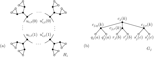
Figure 4: The common vertices are depicted in white. (a) The variable gadget $H_{i}$. (b) The clause gadget $G_{j}$.

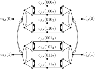
Figure 5: Suppose that the variable $u_{i}$ is the literal $s_{j}$ of the clause $c_{j}$, so $k=yzx_{2}$. We connect $H_{i}$ with $G_{j}$ as depicted. Suppose that an automorphism $\pi$ maps $c_{j,s}(k)$ to $c_{j,s}(k\oplus p)$. We depict the action of $\pi$ on the vertices of $H_{i}$ when $p=001$ (in white), $p=010$ (in gray), and $p=100$ (in black).

Suppose that a variable $u_{i}$ has $o$ literals in the formula. We replace $H_{i}$ by a $4o$-cycle, together with a small gadget attached to each vertex as depicted in Fig. 4a. Suppose that the vertices $u_{i,1}(j),\dots,u_{i,o}(j)$ correspond to $u_{i}(j)$ and similarly $u^{\prime}_{i,1}(j),\dots,u^{\prime}_{i,o}(j)$ correspond to $u^{\prime}_{i}(j)$. The vertices of $4o$-cycle are ordered:

$$u_{i,1}(0),\dots,u_{i,o}(0),u_{i,o}(1),\dots,u_{i,1}(1),u^{\prime}_{i,1}(1),\dots,u^{\prime}_{i,o}(1),u^{\prime}_{i,o}(0),\dots,u^{\prime}_{i,1}(0).$$

We similarly define the automorphisms $\alpha_{i}$ and $\beta_{i}$ and lists for the vertices on the cycle.

Consider the attached gadgets to four vertices corresponding to one literal of a clause $c_{j}$. The vertices depicted in white are adjacent to the added vertices $c_{j,u_{i}}(k)$ of $G_{j}$, as depicted in Fig. 5. Each $k$ consists of three bits, denoted $x$, $y$ and $z$ (in some order). The bit $x$ corresponds to the literal (i.e, the first bit for $u_{i}=q_{j}$, and so on). The white vertices of gadgets attached to $u_{i,t}(j)$ and $u^{\prime}_{i,t}(j)$ are attached to $c_{j,u_{i}}(k)$ where $x=j$. Adjacent pairs of white vertices are connected to $c_{j}(k)$ where $k$ differs in another bit $y$. Non-adjacent pairs of white vertices in one gadget are connected to $c_{j}(k)$ where $k$ differs in the last bit $z$.

In Fig. 5, the action of ${\mathbb{Z}}_{2}^{3}$ is depicted. When $\alpha_{i}$ or $\beta_{i}$ is used on $H_{i}$, they are further composed with the vertical reflection. Therefore, Lemma 7 translated to the modified definitions of variable and clause gadgets which implies correctness of the reduction. The lists for the vertices of the attached gadgets are created by composition of three depicted automorphisms together with $\alpha_{i}$ and $\beta_{i}$; observe that they are of size at most $3$.

The constructed graph $G$ is 3-regular and all lists of $G$ are of size at most $3$. We color the vertices by the orbits of all list-compatible automorphisms and their compositions. Notice that each color class is of size at most $16$. More precisely, all color classes on each $H_{i}$ are of size $16$, and all color classes of clause gadgets $G_{j}$ are of size $8$. ∎

With Lemma 6, we get a dichotomy for the maximum degree: ListIso can be solved in time ${\mathcal{O}}(\sqrt{n}\ell)$ for the maximum degree 2, and it is NP-complete for the maximum degree 3. Similarly, Lemma 3 implies a dichotomy for the list sizes: ListIso can be solved in time ${\mathcal{O}}(n+m)$ where all lists are of size 2, and it is NP-complete for lists of size at most 3. For the last parameter, the maximum size of color classes, there is a gap. Lemma 3 implies that ListIso can be solved in time ${\mathcal{O}}(n+m)$ when all color classes are of size 2 while it is NP-complete for size at most 16.

6 Trees

In this section, we modify the standard algorithm for tree isomorphism to solve list restricted isomorphism of trees. We may assume that both trees $G$ and $H$ are rooted, otherwise we root them by their centers (and possibly subdivide the central edges). The algorithm for GraphIso process both trees from bottom to the top. Using dynamic programming, it computes for every vertex possible images using possible images of its children. This algorithm can be modified to ListIso.

Theorem 6.1

The problem ListIso can be solved for trees in time ${\mathcal{O}}(\sqrt{n}\ell)$.

Proof

We apply the same approach with lists and update these lists as we go from bottom to the top. After processing a vertex $u$, we compute an updated list ${\mathfrak{L}}^{\prime}(u)$ which contains all elements of ${\mathfrak{L}}(u)$ to which $u$ can be mapped compatibly with its descendants. To initiate, each leaf $u$ of $G$ has ${\mathfrak{L}}^{\prime}(u)=\{w:\text{$w$ is a leaf and $w\in{\mathfrak{L}}(u)$}\}$.

Next, we want to compute ${\mathfrak{L}}^{\prime}(u)$ and we know ${\mathfrak{L}}^{\prime}(u_{i})$ of all children $U=\{u_{1},\dots,u_{k}\}$ of $u$. For each $w\in{\mathfrak{L}}(u)$ with $k$ children $w_{1},\dots,w_{k}$, we want to decide whether to put $w\in{\mathfrak{L}}^{\prime}(u)$. Let $W=\{w_{1},\dots,w_{k}\}$. Each $u_{i}$ can be mapped to all vertices in ${\mathfrak{L}}^{\prime}(u_{i})\cap W$. We need to decide whether all $u_{i}$’s can be mapped simultaneously. Therefore, we form a bipartite graph $B(U,W)$ between $U$ and $W$: we put an edge $u_{i}w_{j}$ if and only if $w_{j}\in{\mathfrak{L}}^{\prime}(u_{i})$. Simultaneous mapping is possible if and only if there exists a perfect matching in this bipartite graph.

Let $r$ be the root of $G$ and $r^{\prime}$ be the root of $H$. We claim that there is a list-compatible isomorphism $\pi:G\to H$, if and only if ${\mathfrak{L}}^{\prime}(r)=\{r^{\prime}\}$. Suppose that $\pi$ exists. When $\pi(u)=w$, its children $U$ are mapped to $W$. Since this mapping is compatible with the lists, $w\in{\mathfrak{L}}(u)$, and the mapping of $u_{1},\dots,u_{k}$ gives a perfect matching in $B(U,W)$. Therefore, $w\in{\mathfrak{L}}^{\prime}(u)$, and by induction $r^{\prime}\in{\mathfrak{L}}^{\prime}(r)$. On the other hand, we can construct $\pi$ from the top to the bottom. We start by putting $\pi(r)=r^{\prime}$. When $\pi(u)=w$, we map its children $U$ to $W$ according to some perfect matching in $B(U,W)$ which exists from the fact that $w\in{\mathfrak{L}}^{\prime}(u)$.

It remains to argue details of the complexity. We process the tree which takes time ${\mathcal{O}}(\ell)$ (assuming $n\leq\ell$) and we process each list constantly many times which takes ${\mathcal{O}}(\ell)$. Suppose that we want to compute ${\mathfrak{L}}^{\prime}(u)$. We consider all vertices $w^{1},\dots,w^{p}\in{\mathfrak{L}}(u)$, and let $W^{j}$ be the children of $w^{j}$. We go through all lists of ${\mathfrak{L}}^{\prime}(u_{1}),\dots,{\mathfrak{L}}^{\prime}(u_{k})$ in linear time, and split them into sublists ${\mathfrak{L}}^{\prime}(u_{i}^{j})$ of vertices whose parent is $w^{j}$. Only these sublists are used in the construction of the bipartite graph $B(U,W^{j})$. Using Lemma 1, we decide existence of a perfect matching in time ${\mathcal{O}}(\sqrt{k}\ell_{j})$ which is at most ${\mathcal{O}}(\sqrt{n}\ell_{j})$, where $\ell_{j}$ is the total size of all sublists ${\mathfrak{L}}^{\prime}(u_{i}^{j})$. When we sum this complexity for all vertices $u$, we get the total running time ${\mathcal{O}}(\sqrt{n}\ell)$.∎

7 Planar Graphs

In this section, we describe how to solve ListIso on planar graphs.

For the purpose of this section, we need to consider a more general definition of a graph. We work with multigraphs and we admit pendant edges with free ends (which are edges attached to single vertices). Also, each edge $uv$ gives rise to two incident darts, one attached to $u$, the other to $v$. Every isomorphism maps vertices and darts while preserving incidencies. We consider the problem ListIso with lists on both vertices and darts.

3-connected Planar Graphs. We have a unique embedding into the sphere (up to the reflection). This embeddings can be described in the language of flags, which are pairs $(d,f)$ where $d$ is a dart and $f$ is an incident face. Every automorphism of $G$ corresponds either to a direct map automorphism, or to a indirect map automorphism (composed with a reflection). In particular, ${\rm Aut}(G)\cong{\rm Aut}({\mathcal{M}})$ acts semiregularly on the set of flags of ${\mathcal{M}}$. See [47] for more details and references. Therefore, if the images of two consecutive darts in the rotational scheme are set, the entire mapping is determined and we just need to check whether it is an isomorphism.

Lemma 9

The problem ListIso (with lists on both vertices and darts) can be solved for 3-connected planar graphs in time ${\mathcal{O}}(\ell)$.

Proof

We start by computing embeddings of both $G$ and $H$, in time ${\mathcal{O}}(n)$. It remains to decide whether there exists a list-compatible isomorphism which has to be a map isomorphism. By Euler Theorem, we know that the average degree is less than six. Consider all vertices of degree at most 5, let $u$ be such a vertex with a smallest list, and let $k=|{\mathfrak{L}}(u)|$. We have $\ell=\Omega(kn)$ and we show that we can decide existence of a list-compatible isomorphism in time ${\mathcal{O}}(kn)$.

We test all possible mappings $\pi:G\to H$ having $\pi(u)\in{\mathfrak{L}}(u)$. For each, we have at most 10 possible ways how to extend this mapping on the neighbors of $u$, and the rest of the mapping is uniquely determined by the embeddings and can be computed in time ${\mathcal{O}}(n)$. In the end, we test whether the constructed mapping $\pi$ is an isomorphism and whether it is list-compatible.∎

3-connected Reduction. A seminal paper by Trakhtenbrot [77] introduced reduction which decomposes a graph into its 3-connected components. This idea was further extended in [78, 42, 39, 15, 82]. We use an augmentation described in [24, 25, 47] which behaves well with respect to automorphism groups.

The reduction is constructed by replacing atoms by colored possibly directed edges. Atoms are subgraphs of the following three types (for precise definitions, see [25]):

• Block atom. Either a pendant star, or a pendant block with attached single pendant edges.

• Proper atom. Inclusion minimal subgraphs separated by a 2-cut.

• Dipoles. They are two vertices together with all (at least two) parallel edges between them.

Further, each atom $A$ has the boundary $\partial A$ (of size at most 2) and the interior $\mathring{A}$. A graph is called essentially 3-connected if it is a 3-connected graph with attached single pendant edges attached. Similarly, a graph is called essentially a cycle if it is a cycle with attached single pendant edges. It follows from [25] that each block atom is either a star, or essentially a cycle, or essentially 3-connected, or $K_{2}$ with a single pendant edge attached. For a proper atom $A$ with $\partial A=\{u,v\}$, we denote by $A^{+}$ the graph with the added edge $uv$. The graph $A^{+}$ is always either essentially a cycle, or essentially 3-connected.

A proper atom or a dipole $A$ is called symmetric if there exists an automorphism in ${\rm Aut}(A)$ exchanging $\partial A$, and asymmetric otherwise. Every block atom is symmetric by the definition. The reduction is done by finding all atoms in $G$ (by [25], they have disjoint interiors) and replacing their interiors by edges. Further, we color these edges to code isomorphism types of atoms, and we use directed edges for asymmetric atoms. Block atoms are replaced by pendant edges with free ends.

We repeat this reductions over and over, which gives a sequence of graphs $G=G_{0},\dots,G_{r}$ where $G_{r}$ is called primitive and contains no atoms. By [25], it is either essentially 3-connected, essentially a cycle, $K_{2}$ possibly with attached single pendant edges, or $K_{1}$ with an attached single pendant edge with a free end. Further, this reduction process can be encoded by the reduction tree $T_{G}$; see Fig. 6 for an example. It is a rooted tree, where each node is labeled by a graph. The root of $T_{G}$ is the primitive graph $G_{r}$. The other nodes correspond to atoms obtained in the reductions. When the interior of an atom $A$ is replaced by an edge $e$, we attach the node representing to $A$ to the edge $e$.

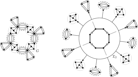
Figure 6: A graph $G$ together with its reduction tree $T_{G}$.

It easily follows that the reduction tree is unique and canonical. Further each automorphism $\pi$ of $G$ induces automorphisms of $G_{1},\dots,G_{r}$ by permuting edges exactly as atoms. Therefore, it induces an automorphism $\pi^{\prime}$ of $T_{G}$ which permutes the nodes of isomorphic graphs, and when it maps a colored edge $e$ to a colored edge $e^{\prime}$, it maps the subtree attached to $e$ to the isomorphic subtree attached to $e^{\prime}$. And every automorphism of $G$ can be constructed in this way, from the root of $T_{G}$ to the bottom. We can use this to solve ListIso.

Theorem 7.1

Let ${\mathcal{C}}$ be a class of graphs closed under contractions and removing vertices. Suppose that ListIso with lists on both vertices and darts can be solved for 3-connected graphs in ${\mathcal{C}}$ in time $\varphi(n,m,\ell)$. We can solve ListIso on ${\mathcal{C}}$ in time ${\mathcal{O}}(\sqrt{m}\ell+m+\varphi(n,m,\ell))$.

Proof

We compute reduction trees $T_{G}$ and $T_{H}$ for both $G$ and $H$ in time ${\mathcal{O}}(n+m)$. We apply the idea of Theorem 6.1 to test list-compatible isomorphism of $T_{G}$ and $T_{H}$. We compute the lists ${\mathfrak{L}}(N)$ for the nodes $N$ of $T_{G}$, from the bottom to the root. A node $M\in{\mathfrak{L}}(N)$ if there exists a list-compatible isomorphism from $N$ to $M$ mapping $\partial N$ to $\partial M$ and there exists list-compatible isomorphism between attached subtrees. (Further, if $|\partial N|=|\partial M|=2$, we remember in ${\mathfrak{L}}(N)$ which of both possible mappings of $\partial N$ to $\partial M$ can be extended as list-compatible isomorphisms.)

Suppose that $N$ has the children $N_{1},\dots,N_{k}$ with computed lists and $M$ has the children $M_{1},\dots,M_{k}$. There exists a list-compatible isomorphism mapping the subtree of $N_{i}$ to the subtree of $M_{j}$, if and only if $M_{j}\in{\mathfrak{L}}(N_{i})$. The difference from Theorem 6.1 is these subtrees have to be compatible with a list-isomorphism from $N$ to $M$; so it depends on the structure of the nodes $N$ and $M$.

There, we compute ${\mathfrak{L}}(N)$ differently according to the type of $N$:

• Star block atoms or dipoles. For star block atoms, similarly as in Theorem 6.1, we construct a bipartite graph between $N_{1},\dots,N_{k}$ and $M_{1},\dots,M_{k}$ and test existence of a perfect matching using Lemma 1. For dipoles, we test two possible isomorphisms, construct two bipartite graph and test existence of perfect matchings.

• Non-star block or proper atoms. We modify the lists of $\partial N$ to the vertices of $\partial M$ only. (When they are proper atoms, we run this in two different ways.) We encode the lists ${\mathfrak{L}}(N_{1}),\dots,{\mathfrak{L}}(N_{k})$ by lists on the corresponding darts of $N$ (depending on which of two possible list-isomorphisms of $\partial N_{i}$ are possible), and we remove single pendant edges, and intersect their lists with the lists of the incident vertices. For a proper atom, we further consider $N^{+}$ and $M^{+}$ with added edges $e$ and $f$ such that ${\mathfrak{L}}(e)=\{f\}$. If the nodes are $K_{2}$ or cycles, and we can test existence of a list-compatible isomorphism using Lemma 5. If both are 3-connected, we can test it by our assumption in time $\varphi(n^{\prime},m^{\prime},\ell^{\prime})$. If this list-compatible isomorphism exists, we add $M$ to ${\mathfrak{L}}(N)$.

• The root primitive graphs. We use the same approach as above, ignoring the part about $\partial N$ and $\partial M$.

A list-compatible isomorphism from $G$ to $H$ exists, if and only if $M\in{\mathfrak{L}}(N)$ for the root nodes $N$ and $M$ of $T_{G}$ and $T_{H}$.

The correctness of the algorithm can be argued from the fact that all automorphisms are captured by the reduction trees [25], inductively from the top to the bottom as in Theorem 6.1. It remains to discuss the running time. The reduction trees can be computed in linear time [39]. When computing ${\mathfrak{L}}(N)$, we first consider the lists of all vertices and edges of $N$. A node $M$ is a candidate for ${\mathfrak{L}}(N)$, if every vertex and every edge of $N$ has a vertex/edge of $M$ in its list. Therefore, we can find all these candidate nodes by iterating these lists, in linear time with respect to their total size. Let $M$ be one of them, and let $n^{\prime}=|V(N)|$, $m^{\prime}=|E(N)|$ and $\ell^{\prime}$ be the total size of lists of the vertices and edges of $N$ when restricted only to the vertices and edges of $M$. Either we construct a bipartite graph and test existence of a perfect matching in time ${\mathcal{O}}(\sqrt{m}^{\prime}\ell^{\prime})$, or we test existence of a list-compatible isomorphism in time $\varphi(n^{\prime},m^{\prime},\ell^{\prime})$. The total running time spent on the tree is ${\mathcal{O}}(\ell)$, the total running time spent testing perfect matchings is ${\mathcal{O}}(\sqrt{m}\ell)$, and the total running time testing list-compatible isomorphisms of 3-connected graphs is ${\mathcal{O}}(\varphi(n,m,\ell))$.∎

General Planar Graphs. By putting both results together, we get the following result:

Theorem 7.2

The problem ListIso can be solved for planar graphs in time ${\mathcal{O}}(\sqrt{n}\ell)$.

Proof

If $G$ and $H$ are connected, we use Theorem 7.1. By Lemma 9, the function $\varphi(n,m,\ell)$ is ${\mathcal{O}}(\ell)$. If $G$ and $H$ are disconnected, we apply Lemma 4 on all connected components of $G$ and $H$, and by analysing the proof, the total running time is ${\mathcal{O}}(\sqrt{n}\ell)$.∎

8 Interval, Permutation and Circle Graphs

In this section, we prove that the standard algorithms solving GraphIso on interval, circle and permutation graphs can be modified to solve ListIso on them. The key idea is that the structure of these graph classes can be captured by graph-labeled trees which are unique up to isomorphism and which capture the structure of all automorphisms; see [48, 49] and the references therein.

For interval graphs, we use MPQ-tree. For circle graphs, we use split trees. For permutation graphs, we use modular trees. On these trees, we apply bottom-up procedure similarly as in the proof of Theorem 6.1. The key difference is that nodes correspond to either prime, or degenerate graphs. Degenerate graphs are simpler and lead to perfect matchings in bipartite graphs. Prime graphs have a small number of automorphisms [48, 49], so all of them can be tested.

8.1 Interval Graphs

To each interval graph $G$, a unique MPQ-tree $T_{G}$ is assigned. Two interval graphs $G$ and $H$ are isomorphic if and only if $T_{G}$ and $T_{H}$ are equivalent, and these trees capture all isomorphisms. Therefore, we apply a bottom-up proceduce to test ListIso for MPQ-trees, similarly as in Theorem 6.1.

MPQ-trees. Booth and Lueker [10] invented a data structure called a PQ-tree which capture the structure of an interval graph. We use modified PQ-trees (MPQ-trees) due to Korte and Möhring [53]. Let $G$ be an interval graph. A rooted tree $T$ is an MPQ-tree if the following holds. It has two types of inner nodes: P-nodes and Q-nodes. For every inner node, its children are ordered from left to right. Each P-node has at least two children and each Q-node at least three. The leaves of $T$ correspond one-to-one to the maximal cliques in $G$.

Two MPQ-trees are equivalent if one can be obtained from the other by a sequence of two equivalence transformations: (i) an arbitrary permutation of the order of the children of a P-node, and (ii) the reversal of the order of the children of a Q-node. Booth and Lueker [10] proved the existence and uniqueness of PQ-trees (up to equivalence transformations); see Fig. 7.

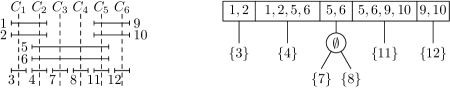
Figure 7: An ordering of the maximal cliques, and the corresponding MPQ-tree. The P-nodes are denoted by circles, the Q-nodes by rectangles. There are four equivalent MPQ-trees.

We assign subsets of $V(G)$, called sections, to the nodes of $T$; see Fig. 7. The leaves and the P-nodes have each assigned exactly one section while the Q-nodes have one section per child. We assign these sections as follows:

• For a leaf $L$, the section ${\rm sec}(L)$ contains those vertices that are only in the maximal clique represented by $L$, and no other maximal clique.

• For a P-node $P$, the section ${\rm sec}(P)$ contains those vertices that are in all maximal cliques of the subtree of $P$, and no other maximal clique.

• For a Q-node $Q$ and its children $T_{1},\dots,T_{n}$, the section ${\rm sec}_{i}(Q)$ contains those vertices that are in the maximal cliques represented by the leaves of the subtree of $T_{i}$ and also some other $T_{j}$, but not in any other maximal clique outside the subtree of $Q$. We put ${\rm sec}(Q)={\rm sec}_{1}(Q)\cup\cdots\cup{\rm sec}_{n}(Q)$.

Each vertex appears in sections of exactly one node and in the case of a Q-node in consecutive sections. Two vertices are in the same sections if and only if they belong to precisely the same maximal cliques. Figure 7 shows an example. MPQ-tree can be constructed in time [53].

Testing ListIso. Let $G$ and $H$ be two isomorphic interval graphs. From [49, Lemma 4.3], it follows that $T_{G}$ and $T_{H}$ are equivalent, and every isomorphism $\pi:G\to H$ is obtained by an equivalence transformation of $T_{G}$ and some permutation of the vertices in identical sections. Now, we are ready to show ListIso can be solved on interval graphs in time ${\mathcal{O}}(\sqrt{n}\ell+m)$:

Theorem 8.1

The problem ListIso can be solved for interval graphs in time ${\mathcal{O}}(\sqrt{n}\ell+m)$.

Proof

We proceed similarly as in Theorem 6.1. We compute MPQ-trees representing $T_{G}$ and $T_{H}$ representing the graphs $G$ and $H$ in linear time [53]. Then we compute lists ${\mathfrak{L}}(N)$ for every node $N$ of $T_{G}$ from the bottom. We distinguish three types of nodes.

• Leaf nodes. Let $L_{G}$ be a leaf node in $T_{G}$ and let $L_{H}$ be a leaf node in $T_{H}$. Then $L_{H}\in{\mathfrak{L}}(L_{G})$ if there exists a list-compatible isomorphism between the induced complete subgraphs $G[{\rm sec}(L_{G})]$ and $H[{\rm sec}(L_{H})]$.

• P-nodes. Let $N$ and $M$ be P-nodes of $T_{G}$ and $T_{H}$, respectively. We want to decide whether $M\in{\mathfrak{L}}(N)$. Let $N_{1},\dots,N_{k}$ be the children of $N$ and let $M_{1},\dots,M_{k}$ be the children of $M_{k}$. We construct a bipartite graph similarly as in Theorem 6.1. Then $M\in{\mathfrak{L}}(N)$ if there exists a perfect matching in the bipartite graph and a perfect matching between the lists of $G[{\rm sec}(N)]$ and $H[{\rm sec}(M)]$ (which are complete graphs).

• Q-nodes. Let $N$ and $M$ be Q-nodes of $T_{G}$ and $T_{H}$ and let $N_{1},\dots,N_{k}$ and $M_{1},\dots,M_{k}$ be their children. Here we have at most two possible isomorphisms. In particular, an isomorphism can either map the subtree of $N_{i}$ on the subtree of $M_{i}$, or in the reversed order, and we can test for both possibilities whether the lists ${\mathfrak{L}}(N_{i})$ are compatible. Moreover, we consider all sets of intervals belonging to exactly the same sections of the Q-node, and we test by perfect matchings between pairs of them whether there exists a list-compatible isomorphism between them.

The MPQ-trees have ${\mathcal{O}}(n)$ nodes and ${\mathcal{O}}(n)$ intervals in their sections. For leaf nodes and P-nodes, the analysis is exactly the same as in the proof of Theorem 6.1. For Q-nodes, we just test two possible mappings and bipartite matchings for sections. We get the total running time ${\mathcal{O}}(\sqrt{n}\ell+m)$.∎

8.2 Permutation Graphs

A module $M$ of a graph $G$ is a set of vertices such that each $x\in V(G)\setminus M$ is either adjacent to all vertices in $M$, or to none of them. See Fig. 8a for examples. A module $M$ is called trivial if $M=V(G)$ or $|M|=1$, and non-trivial otherwise. If $M$ and $M^{\prime}$ are two disjoint modules, then either the edges between $M$ and $M^{\prime}$ form the complete bipartite graph, or there are no edges at all; see Fig. 8a. In the former case, $M$ and $M^{\prime}$ are called adjacent, otherwise they are non-adjacent.

Figure 8: (a) A graph $G$ with a modular partition ${\mathcal{P}}$. (b) The quotient graph $G/{\mathcal{P}}$ is prime.

Let ${\mathcal{P}}=\{M_{1},\dots,M_{k}\}$ be a modular partition of $V(G)$, i.e., each $M_{i}$ is a module of $G$, $M_{i}\cap M_{j}=\emptyset$ for every $i\neq j$, and $M_{1}\cup\cdots\cup M_{k}=V(G)$. We define the quotient graph $G/{\mathcal{P}}$ with the vertices $m_{1},\dots,m_{k}$ corresponding to $M_{1},\dots,M_{k}$ where $m_{i}m_{j}\in E(G/{\mathcal{P}})$ if and only if $M_{i}$ and $M_{j}$ are adjacent. In other words, the quotient graph is obtained by contracting each module $M_{i}$ into the single vertex $m_{i}$; see Fig. 8b.

Modular Decomposition. To decompose $G$, we find some modular partition ${\mathcal{P}}=\{M_{1},\dots,M_{k}\}$, compute $G/{\mathcal{P}}$ and recursively decompose $G/{\mathcal{P}}$ and each $G[M_{i}]$. The recursive process terminates on prime graphs which are graphs containing only trivial modules. There might be many such decompositions for different choices of ${\mathcal{P}}$ in each step. In 1960s, Gallai [31] described the modular decomposition in which special modular partitions are chosen and which encodes all other decompositions.

The key is the following observation. Let $M$ be a module of $G$ and let $M^{\prime}\subseteq M$. Then $M^{\prime}$ is a module of $G$ if and only if it is a module of $G[M]$. A graph $G$ is called degenerate if it is $K_{n}$ or $\overline{K}_{n}$. We construct the modular decomposition of a graph $G$ in the following way, see Fig. 9a for an example:

• If $G$ is a prime or a degenerate graph, then we terminate the modular decomposition on $G$. We stop on degenerate graphs since every subset of vertices forms a module, so it is not useful to further decompose them.

• Let $G$ and $\overline{G}$ be connected graphs. Gallai [31] shows that the inclusion maximal proper subsets of $V(G)$ which are modules form a modular partition ${\mathcal{P}}$ of $V(G)$, and the quotient graph $G/{\mathcal{P}}$ is a prime graph; see Fig. 8. We recursively decompose $G[M]$ for each $M\in{\mathcal{P}}$.

• If $G$ is disconnected and $\overline{G}$ is connected, then every union of connected components is a module. Therefore the connected components form a modular partition ${\mathcal{P}}$ of $V(G)$, and the quotient graph $G/{\mathcal{P}}$ is an independent set. We recursively decompose $G[M]$ for each $M\in{\mathcal{P}}$.

• If $\overline{G}$ is disconnected and $G$ is connected, then the modular decomposition is defined in the same way on the connected components of $\overline{G}$. They form a modular partition ${\mathcal{P}}$ and the quotient graph $G/{\mathcal{P}}$ is a complete graph. We recursively decompose $G[M]$ for each $M\in{\mathcal{P}}$.

Modular Tree. We encode the modular decomposition by the modular tree $T$. The modular tree $T$ is a graph with two types of vertices (normal and marker vertices) and two types of edges (normal and directed tree edges). The directed tree edges connect the prime and degenerate graphs encountered in the modular decomposition (as quotients and terminal graphs) into a rooted tree.

We give a recursive definition. Every modular tree has an induced subgraph called root node. If $G$ is a prime or a degenerate graph, we define $T=G$ and its root node equals $T$. Otherwise, let ${\mathcal{P}}=\{M_{1},\dots,M_{k}\}$ be the used modular partition of $G$ and let $T_{1},\dots,T_{k}$ be the modular trees corresponding to $G[M_{1}],\dots,G[M_{k}]$. The modular tree $T$ is the disjoint union of $T_{1},\dots,T_{k}$ and of $G/{\mathcal{P}}$ with the marker vertices $m_{1},\dots,m_{k}$. To every graph $T_{i}$, we add a new marker vertex $m^{\prime}_{i}$ such that $m^{\prime}_{i}$ is adjacent exactly to the vertices of the root node of $T_{i}$. We further add a tree edge oriented from $m_{i}$ to $m^{\prime}_{i}$. For an example, see Fig. 9b.

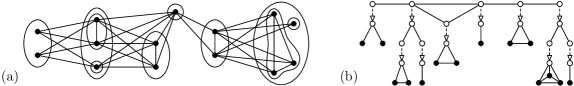
Figure 9: (a) The graph $G$ from Fig. 8 with the modular partitions used in the modular decomposition. (b) The modular tree $T$ of $G$, the marker vertices are white, the tree edges are dashed.

The modular tree of $G$ is unique. The graphs encountered in the modular decomposition are called nodes of $T$, or alternatively root nodes of some modular trees in the construction of $T$. For a node $N$, its subtree is the modular tree which has $N$ as the root node. Leaf nodes correspond to the terminal graphs in the modular decomposition, and inner nodes are the quotients in the modular decomposition. All vertices of $G$ are in leaf nodes and all marker vertices correspond to modules of $G$. All inner nodes consist of marker vertices.

Testing ListIso. Now, we are ready to show that the problem ListIso can be decided in ${\mathcal{O}}(\sqrt{n}\ell+m)$ time for permutation graphs.

Theorem 8.2

The problem ListIso can be solved for permutation graphs in time ${\mathcal{O}}(\sqrt{n}\ell+m)$.

Proof

For input graph $G$ and $H$, we first compute the modular trees $T_{G}$ and $T_{H}$, respectively, in time ${\mathcal{O}}(n+m)$ [64]. We again apply the idea of Theorem 6.1. We compute the list ${\mathfrak{L}}(N)$ for every node $N$ of $T_{G}$. Note that all inner nodes consist only of marker vertices which have no lists. Therefore, we first compute ${\mathfrak{L}}(L)$, for every leaf node. A leaf node $K$ is in ${\mathfrak{L}}(L)$ if every non-marker vertex of $L$ has a non-marker vertex of $K$ in its list. These candidate nodes for ${\mathfrak{L}}(L)$ can be found in linear time in the total size of lists by iterating through the lists of vertices of $L$.

Suppose that a node $N$ has the children $N_{1},\dots,N_{k}$ with computed lists ${\mathfrak{L}}(N_{1}),\dots,{\mathfrak{L}}(N_{k})$ and $M$ has the children $M_{1},\dots,M_{k}$. There exist a list-compatible isomorphism mapping the subtree of $N_{i}$ to the subtree of $M_{j}$ if and only if $M_{j}\in{\mathfrak{L}}(N_{i})$. Moreover these subtrees have to be compatible with a list isomorphism from $N$ to $M$. We compute ${\mathfrak{L}}(N)$ according to the type of $N$.

• Degenerate nodes. For degenerate nodes, we proceed similarly as for trees in Theorem 6.1. We construct a bipartite graph between the nodes nodes $N_{1},\dots,N_{k}$ and $M_{1},\dots,M_{k}$ and test for a perfect matching using Lemma 1.

• Prime nodes. For prime nodes, there are at most four possible isomorphisms mapping $N$ to $M$ [49, Lemma 6.6]. We test for these four possible isomorphisms $\pi$ whether $\pi(M_{i})\in{\mathfrak{L}}(M_{i})$ for every $M_{i}$.

A list compatible isomorphism exists if $M\in{\mathfrak{L}}(N)$, for the root nodes $N$ and $M$ of $T_{G}$ and $T_{H}$. The correctness of the algorithm follows from the fact that all automorphisms of a permutation graph are captured by the modular tree [49]. A similar argument as in the proofs of Theorems 6.1 and 8.1 gives the running time.∎

8.3 Circle Graphs

For a given circle graph, we define the split tree which captures its automorphism group. A split is a partition $(A,B,A^{\prime},B^{\prime})$ of $V(G)$ such that:

• For every $a\in A$ and $b\in B$, we have $ab\in E(G)$.

• There are no edges between $A^{\prime}$ and $B\cup B^{\prime}$, and between $B^{\prime}$ and $A\cup A^{\prime}$.

• Both sides have at least two vertices: $|A\cup A^{\prime}|\geq 2$ and $|B\cup B^{\prime}|\geq 2$.

The split decomposition of $G$ is constructed by taking a split of $G$ and replacing $G$ by the graphs $G_{A}$ and $G_{B}$ defined as follows. The graph $G_{A}$ is created from $G[A\cup A^{\prime}]$ together with a new marker vertex $m_{A}$ adjacent exactly to the vertices in $A$. The graph $G_{B}$ is defined analogously for $B$, $B^{\prime}$ and $m_{B}$; see Fig. 10a. The decomposition is then applied recursively on $G_{A}$ and $G_{B}$. Graphs containing no splits are called prime graphs. We stop the split decomposition also on degenerate graphs which are complete graphs $K_{n}$ and stars $K_{1,n}$. A split decomposition is called minimal if it is constructed by the least number of splits. Cunningham [16] proved that the minimal split decomposition of a connected graph is unique.

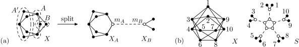
Figure 10: (a) An example of a split of the graph $G$. The marker vertices are depicted in white. The tree edge is depicted by a dashed line. (b) The split tree $S$ of the graph $G$. We have that ${\rm Aut}(S)\cong\mathbb{Z}_{2}^{5}\rtimes\mathbb{D}_{5}$.

Split tree. The split tree $T$ representing a graph $G$ encodes the minimal split decomposition. A split tree is a graph with two types of vertices (normal and marker vertices) and two types of edges (normal and tree edges). We initially put $T=G$ and modify it according to the minimal split decomposition. If the minimal decomposition contains a split $(A,B,A^{\prime},B^{\prime})$ in $G$, then we replace $G$ in $T$ by the graphs $G_{A}$ and $G_{B}$, and connect the marker vertices $m_{A}$ and $m_{B}$ by a tree edge (see Fig. 10a). We repeat this recursively on $G_{A}$ and $G_{B}$; see Fig. 10b. Each prime and degenerate graph is a node of the split tree. A node that is incident with exactly one tree edge is called a leaf node.

Since the minimal split decomposition is unique, we also have that the split tree is unique. Further, each automorphism $\pi$ of $G$ induces an automorphism $\pi^{\prime}$ of the split tree $T$ representing $G$. Similarly as for trees, there exists a center of $T$ which is either a tree edge, or a prime or degenerate node. The automorphism $\pi^{\prime}$ preserves the center, so we can regard $T$ as rooted by the center. Every automorphism of $G$ can be reconstructed from the root of $T$ to the bottom.

Testing ListIso. Next, we show that the problem ListIso can be solved on circle graphs in time ${\mathcal{O}}(\sqrt{n}\ell+m\cdot\alpha(m)$.

Theorem 8.3

The problem ListIso can be solved for circle graphs in time ${\mathcal{O}}(\sqrt{n}\ell+m\cdot\alpha(m))$, where $\alpha$ is the inverse Ackermann function.

Proof

For input graph $G$ and $H$, we first compute the split trees $T_{G}$ and $T_{H}$, in time ${\mathcal{O}}((n+m)\cdot\alpha(n+m))$ [32]. We assume that the trees $T_{G}$ and $T_{H}$ are rooted and we can also assume that the roots are prime or degenerate nodes. We again apply the idea of Theorem 6.1.

We compute the list ${\mathfrak{L}}(N)$ for every node $N$ of $T_{G}$. Let $M$ be a leaf node of $T_{H}$ and let $m_{N}\in V(N)$ and $m_{M}\in V(M)$ be the marker vertices incident to a tree edge closer to the root. Then $M$ is in ${\mathfrak{L}}(N)$ if there is a list-compatible isomorphism from $N$ to $M$ which maps $m_{N}$ to $m_{M}$.

Suppose that a node $N$ has the children $N_{1},\dots,N_{k}$ with computed lists ${\mathfrak{L}}(N_{1}),\dots,{\mathfrak{L}}(N_{k})$ and $M$ has the children $M_{1},\dots,M_{k}$. There exist a list-compatible isomorphism mapping the subtree of $N_{i}$ to the subtree of $M_{j}$ if and only if $M_{j}\in{\mathfrak{L}}(N_{i})$. Moreover these subtrees have to be compatible with an isomorphism from $N$ to $M$. We compute ${\mathfrak{L}}(N)$ according to the type of $N$.

• Degenerate nodes. For degenerate nodes, we proceed similarly as for trees in Theorem 6.1. We construct a bipartite graph between the nodes nodes $N_{1},\dots,N_{k}$ and $M_{1},\dots,M_{k}$ and test for a perfect matching using Lemma 1.

• Prime nodes. For prime nodes, there are at most four possible isomorphisms mapping $m_{N}$ to $m_{M}$ [48, Lemma 5.6]. We test those four possible isomorphisms, construct four bipartite graphs and test existence of perfect matchings.

• The root node. If it is degenerate, we proceed as above. If it is prime, then its automorphism groups is a subgroup of a dihedral group [48, Lemma 5.5]; essentially it behaves as a cycle. Therefore, we approach it similarly as in Lemma 5.

A list compatible isomorphism exists if $M\in{\mathfrak{L}}(N)$, for the root nodes $N$ and $M$ of $T_{G}$ and $T_{H}$.

The correctness of the algorithm follows from the fact that all automorphisms of a circle graph are captured by the split tree [48]. The running time can be argued as in Theorems 6.1, 8.1, and 8.2.∎

9 Bounded Genus Graphs

In this section, we describe an FPT algorithm solving ListIso when parameterized by the Euler genus $g$. We modify the recent paper of Kawarabayashi [46] solving graph isomorphism in linear time for a fixed genus $g$. The harder part of this paper are structural results, described below, which transfer to list-compatible isomorphisms without any change. Using these structural results, we can build our algorithm.

Theorem 9.1

For every integer $g$, the problem ListIso can be solved on graphs of Euler genus at most $g$ in time ${\mathcal{O}}(\sqrt{n}\ell)$.

Proof

See [46, p. 14] for overview of the main steps. We show that these steps can be modified to deal with lists. We prove this result by induction on $g$, where the base case for $g=0$ is Theorem 7.2. Next, we assume that both graphs $G$ and $H$ are 3-connected, otherwise we apply Theorem 7.1. By [46, Theorem 1.2], if $G$ and $H$ have no polyhedral embeddings, then the face-width is at most two.

Case 1: $G$ and $H$ have polyhedral embeddings. Following [46, Theorem 1.2], we have at most $f(g)$ possible embeddings of $G$ and $H$. We choose one embedding of $G$ and we test all embeddings of $H$. It is known that the average degree is ${\mathcal{O}}(g)$. Therefore, we can apply the same idea as in the proof of Lemma 9 and test isomorphism of all these embeddings in time ${\mathcal{O}}(\ell)$.

Case 2: $G$ and $H$ have no polyhedral embedding, but have embeddings of face-width exactly two. Then we split $G$ into a pair of graphs $(G^{\prime},L)$. The graph $L$ are called cylinders and the graph $G^{\prime}$ correspond to the remainder of $G$. The following properties hold [46, p. 5]:

• We have $G=G^{\prime}\cup L$ and for $\partial L=V(G^{\prime}\cap L)$, we have $|\partial L|=4$.

• The graph $G^{\prime}$ can be embedded to a surface of genus at most $g-1$, and $L$ is planar [46, p. 4].

• This pair $(G^{\prime},L)$ is canonical, i.e., every isomorphism from $G$ to $H$ maps $(G^{\prime},L)$ to another pair $(H^{\prime},L^{\prime})$ in $H$.

It is proved [46, Theorem 5.1] that there exists some function $q^{\prime}(g)$ bounding the number of these pairs both in $G$ and $H$, and can be found in time ${\mathcal{O}}(n)$. We fix a pair $(G^{\prime},L)$ in $G$ and iterate over all pairs $(H^{\prime}_{i},L^{\prime}_{i})$ in $H$. Following [46, p. 36], we get that $G\cong H$, if and only if there exists a pair $(H^{\prime}_{i},L^{\prime}_{i})$ in $H$ such that $G^{\prime}\cong H^{\prime}_{i}$, $L\cong L^{\prime}_{i}$, and $G^{\prime}\cap L$ is mapped to $H^{\prime}_{i}\cap L^{\prime}_{i}$. To test this, we run at most $2q^{\prime}(g)$ instances of ListIso on smaller graphs with modified lists.

Suppose that we want to test whether $G^{\prime}\cong H^{\prime}_{i}$ and $L\cong L^{\prime}_{i}$. First, we modify the lists: for $u\in V(G^{\prime})$, put ${\mathfrak{L}}^{\prime}(u)={\mathfrak{L}}(u)\cap H^{\prime}_{i}$, and for $v\in V(L)$, put ${\mathfrak{L}}^{\prime}(v)={\mathfrak{L}}(v)\cap L^{\prime}_{i}$, and similarly for lists of darts. Further, for all vertices $u\in\partial L$ in both $G^{\prime}$ and $L$, we put ${\mathfrak{L}}^{\prime}(u)={\mathfrak{L}}(u)\cap\partial L$. We test existence of list-compatible isomorphisms from $G^{\prime}$ to $H^{\prime}_{i}$ and from $L$ to $L^{\prime}_{i}$. There exists a list-compatible isomorphism from $G$ to $H$, if and only if these list-compatible isomorphisms exist at least for one pair $(H^{\prime}_{i},L^{\prime}_{i})$.

We note that when $g=2$, a special case is described in [46, Theorem 5.3], which is slightly easier and can be modified similarly.

Case 3: $G$ and $H$ have no polyhedral embedding and have only embeddings of face-width one. Let $V$ be the set of vertices in $G$ such that for each $u\in V$, there exists a non-contractible curve passing only through $u$. By [46, Lemma 6.3], $|V|\leq q(g)$ for some function $q$. For $u$, the non-contractible curve divides its edges to two sides, so we can cut $G$ at $u$, and split the incident edges. We obtain a graph $G^{\prime}$ which can be embedded to a surface of genus at most $g-1$.

By [46, Lemma 6.3], we can find all these vertices $V$ and $V^{\prime}$ in $G$ and $H$ in time ${\mathcal{O}}(n)$. We choose $u\in V$ arbitrarily, and we test all possible vertices $v\in V^{\prime}$. Let $G^{\prime}$ be constructed from $G$ by splitting $u$ into new vertices $u^{\prime}$ and $u^{\prime\prime}$, and similarly $H^{\prime}$ be constructed from $H$ by splitting $v$ into new vertices $v^{\prime}$ and $v^{\prime\prime}$. In [46, p. 36], it is stated that $G\cong H$, if and only if there exists a choice of $v\in V^{\prime}$ such that $G^{\prime}\cong H^{\prime}$ and $\{u^{\prime},u^{\prime\prime}\}$ is mapped to $\{v^{\prime},v^{\prime\prime}\}$. Therefore, we run at most $q(g)$ instances of ListIso on smaller graphs with modified lists.

If $v\notin L(u)$, clearly a list-compatible isomorphism is not possible for this choice of $v\in V^{\prime}$. If $v\in L(u)$, we put $L^{\prime}(u^{\prime})=L^{\prime}(u^{\prime\prime})=\{v^{\prime},v^{\prime\prime}\}$. Then there exists a list-compatible isomorphism from $G$ to $H$, if and only if there exists a list-compatible isomorphism from $G^{\prime}$ to $H^{\prime}$.

The correctness of our algorithm follows from [46]. It remains to argue the complexity. Throughout the algorithm, we produce at most $w(g)$ subgraphs of $G$ and $H$, for some function $w$, for which we test list-compatible isomorphisms. Assuming the induction hypothesis, the reduction of graphs to 3-connected graphs can be done in time ${\mathcal{O}}(\sqrt{n}\ell)$. Case 1 can be solved in time ${\mathcal{O}}(\ell)$. Case 2 can be solved in time ${\mathcal{O}}(\sqrt{n}\ell)$. Case 3 can be solved in time ${\mathcal{O}}(\sqrt{n}\ell)$.∎

10 Bounded Treewidth Graphs

In this section, we prove that ListIso can be solved in FPT with respect to the parameter treewidth $\operatorname{tw}(G)$. Unlike in Sections 7 and 8, the difficulty of graph isomorphism on bounded treewidth graphs raises from the fact that tree decomposition is not uniquely determined. We follow the approach of Bodlaender [9] which describes an XP algorithm for GraphIso of bounded treewidth graphs, running in time $n^{{\mathcal{O}}(\operatorname{tw}(G))}$. Then we show that the recent breakthrough by Lokshtanov et al. [59], giving an FPT algorithm for GraphIso, translates as well.

Definition 1

A tree decomposition of a graph $G$ is a pair ${\cal T}=(\{B_{i}\colon i\in I\},T=(I,F)),$ where $T$ is a rooted tree and $\{B_{i}\colon i\in I\}$ is a family of subsets of $V,$ such that

1. for each $v\in V(G)$ there exists an $i\in I$ such that $v\in B_{i}$,

2. for each $e\in E(G)$ there exists an $i\in I$ such that $e\subseteq B_{i}$,

3. for each $v\in V(G),I_{v}=\{i\in I\colon v\in B_{i}\}$ induces a subtree of $T.$

We call the elements $B_{i}$ the nodes, and the elements of the set $F$ the decomposition edges.

We define the width of a tree decomposition ${\cal T}=(\{B_{i}\colon i\in I\},T)$ as $\max_{i\in I}|B_{i}|-1$ and the treewidth $\operatorname{tw}(G)$ of a graph $G$ as the minimum width of a tree decomposition of the graph $G$.

Nice Tree Decompositions. It is common to define a nice tree decomposition of the graph [50]. We naturally orient the decomposition edges towards the root and for an oriented decomposition edge $(B_{j},B_{i})$ from $B_{j}$ to $B_{i}$ we call $B_{i}$ the parent of $B_{j}$ and $B_{j}$ a child of $B_{i}$. If there is an oriented path from $B_{j}$ to $B_{i}$ we say that $B_{j}$ is a descendant of $B_{i}$.

We also adjust a tree decomposition such that for each decomposition edge $(B_{i},B_{j})$ it holds that $\big{|}|B_{i}|-|B_{j}|\big{|}\leq 1$ (i.e. it joins nodes that differ in at most one vertex). The in-degree of each node is at most $2$ and if the in-degree of the node $B_{k}$ is $2$ then for its children $B_{i},B_{j}$ holds that $B_{i}=B_{j}=B_{k}$ (i.e. they represent the same vertex set).

We classify the nodes of a nice decomposition into four classes—namely introduce nodes, forget nodes, join nodes and leaf nodes. We call the node $B_{i}$ an introduce node of the vertex $v$, if it has a single child $B_{j}$ and $B_{i}\setminus B_{j}=\{v\}$. We call the node $B_{i}$ a forget node of the vertex $v$, if it has a single child $B_{j}$ and $B_{j}\setminus B_{i}=\{v\}$. If the node $B_{k}$ has two children, we call it a join node (of nodes $B_{i}$ and $B_{j}$). Finally we call a node $B_{i}$ a leaf node, if it has no child.

Bodlaender’s Algorithm. A graph $G$ has treewidth at most $k$ if either $|V(G)|\leq k$, or there exists a cut set $U\subseteq V(G)$ such that $|U|\leq k$ and each component of $G\setminus U$ together with $U$ has treewidth at most $k$. The set $U$ corresponds to a bag in some tree decomposition of $G$. Bodlaender’s algorithm [9] enumerates all possible cut sets $U$ of size at most $k$ in $G$ (resp. $H$), we denote these $C_{i}$ (resp. $D_{i}$). Furthermore, it enumerates all connected components of $G\setminus C_{i}$ as $C_{i}^{j}$ (resp. of $H\setminus D_{i}$ as $D_{i}^{j}$). We denote by $G[U,W]$ the graph induced by $U\mathbin{\dot{\cup}}W$. The set $W$ is either a connected component or a collection of connected components. We call $U$ the border set.

Lemma 10 ([1, 9])

A graph $G[U,W]$ with at least $k$ vertices has a treewidth at most $k$ with the border set $U$ if and only if there exists a vertex $v\in W$ such that for each connected component $A$ of $G[W\setminus v]$, there is a $k$-vertex cut $C_{s}\subseteq U\cup\{v\}$ such that no vertex in $A$ is adjacent to the (unique) vertex in $(U\cup\{v\})\setminus C_{s}$, and $G[C_{s},A]$ has treewidth at most $k$.

Lemma 11

The problem ListIso can be solved in XP with respect to the parameter treewidth.

Proof

We modify the algorithm of Bodlaender [9]. Let $k=\operatorname{tw}(G)=\operatorname{tw}(H)$. We compute the sets $C_{i},C_{i}^{j}$ for $G$ and the sets $D_{i^{\prime}},D_{i^{\prime}}^{j^{\prime}}$ for $H$; there are $n^{{\mathcal{O}}(k)}$ pairs $(C_{i},C_{i}^{j})$. The pair $(C_{i},C_{i}^{j})$ is compatible if $C_{i}^{j}$ is a connected component of $G^{\prime}\setminus C_{i}$ for some $G^{\prime}\subseteq G$ that arises during the recursive definition of treewidth. Let $f\colon C_{i}\to D_{i^{\prime}}$ be an isomorphism. We say that $(C_{i},C_{i}^{j})\equiv_{f}(D_{i^{\prime}},D_{i^{\prime}}^{j^{\prime}})$ if and only if there exists an isomorphism $\varphi\colon C_{i}\cup C_{i}^{j}\to D_{i^{\prime}}\cup D_{i^{\prime}}^{j^{\prime}}$ such that $\varphi|_{C_{i}}=f$. In other words, $\varphi$ is a partial isomorphism from $G$ to $H$. The change for ListIso is that we also require that both $f$ and $\varphi$ are list-compatible.

The algorithm resolves $(C_{i},C_{i}^{j})\equiv_{f}(D_{i^{\prime}},D_{i^{\prime}}^{j^{\prime}})$ by the dynamic programming, according to the size of $D_{i^{\prime}}^{j^{\prime}}$. If $|C_{i}^{j}|=|D_{i^{\prime}}^{j^{\prime}}|\leq 1$, we can check it trivially in time $k^{{\mathcal{O}}(k)}$. Otherwise, suppose that $|C_{i}^{j}|=|D_{i^{\prime}}^{j^{\prime}}|>1$, and let $m$ be the number of components of $C_{i}^{j}$ (and thus $D_{i^{\prime}}^{j^{\prime}}$). We test whether $f:C_{i}\to D_{i^{\prime}}$ is a list-compatible isomorphism. Let $v\in C_{i}^{j}$ be a vertex given by Lemma 10 (with $U=C_{i}$ and $W=C_{i}^{j}$) and let $C_{s}$ be the corresponding extension of $v$ to a cut set. We compute for all $w\in D_{i^{\prime}}^{j^{\prime}}\cap{\mathfrak{L}}(v)$ all connected components $B_{q}$. From the dynamic programming, we know for all possible extensions $D^{\prime}$ of $w$ to a cut set whether $(C_{m},A_{p})\equiv_{f^{\prime}}(D^{\prime},B_{q})$ with $f^{\prime}(x)=f(x)$ for $x\in C_{i}$ and $f^{\prime}(v)=w$. Finally, we decide whether there exists a perfect matching in the bipartite graph between $(C_{m},A_{p})$’s and $(D^{\prime},B_{q})$’s where the edges are according to the equivalence.∎

Reducing The Number of Possible Bags. Otachi and Schweitzer [68] proposed the idea of pruning the family of potential bags which finally led to an FPT algorithm [59]. A family $\mathcal{B}(G)$, whose definition depends on the graph, is called isomorphism-invariant if for an isomorphism $\phi:G\to G^{\prime}$, we get $\mathcal{B}(G^{\prime})=\phi(\mathcal{B}(G))$, where $\phi(\mathcal{B}(G))$ denotes the family $\mathcal{B}(G)$ with all the vertices of $G$ replaced by their images under $\phi$.

For a graph $G$, a pair $(A,B)$ with $A\cup B=V$ is called a separation if there are no edges between $A\setminus B$ and $B\setminus A$ in $G$. The order of $(A,B)$ is $|A\cap B|$. For two vertices $u,v\in V(G)$, by $\mu(u,v)$ we denote the minimum order of separation $(A,B)$ with $u\in A\setminus B$ and $v\in B\setminus A$. We say a graph $G$ is $k$-complemented if $\mu_{G}(u,v)\geq k)\implies uv\in E(G)$ holds for every two vertices $u,v\in V$. We may canonically modify the input graphs $G$ and $H$ ListIso, by adding these additional edges and making them $k$-complemented.

Theorem 10.1 ([59], Theorem 5.5)

Let $k$ be a positive integer, and let $G$ be a graph on $n$ vertices that is connected and $k$-complemented. There exists an algorithm that computes in time $2^{{\mathcal{O}}(k^{5}\log k)}\cdot n^{3}$ an isomorphism-invariant family of bags $\mathcal{B}$ with the following properties:

1. $|B|\leq{\mathcal{O}}(k^{4})$ for each $B\in\mathcal{B}$,

2. $|\mathcal{B}|\leq 2^{{\mathcal{O}}(k^{5}\log k)}\cdot n^{2}$,

3. Assuming $\operatorname{tw}(G)<k$, the family $\mathcal{B}$ captures some tree decomposition of $G$ that has width ${\mathcal{O}}(k^{4})$.

4. The family $\mathcal{B}$ is closed under taking subsets.

Theorem 10.2

The problem ListIso can be solved in FPT time $2^{{\mathcal{O}}(k^{5}\log k)}n^{5}$ where $k=\operatorname{tw}(G)$.

Proof

We use the algorithm of Lemma 11, where $C_{i}$’s and $D_{i}$’s are from the collection ${\mathcal{B}}$ of Theorem 10.1. The total number of pairs $(C_{i},C_{i}^{j})$ and $(D_{i^{\prime}},D_{i^{\prime}}^{j^{\prime}})$ is bounded by $2^{{\mathcal{O}}(k^{5}\log k)}n^{3}$ [59, p. 20]. The dynamic programming in [59, Theorem 6.2] is done according to the potential function $\Phi(D_{i^{\prime}},D_{i^{\prime}}^{j^{\prime}})=2|D_{i^{\prime}}^{j^{\prime}}|+|D_{i^{\prime}}|$. We use nice tree decompositions, so in each step, the dynamic programming either introduces a new node into the bag $D_{i^{\prime}}$, or moves a node from the bag $D_{i^{\prime}}$ to $D_{i^{\prime}}^{j^{\prime}}$, or joins several pairs with the same bag $D_{i^{\prime}}$. In all these operations, we check existence of a list-compatible isomorphism, using dynamic programming, exactly as in Lemma 11.∎

11 Conclusions

We conclude this paper with description of related results and open problems.

Forbidden Images. We note that Lubiw [60] used a different definition of ListIso: for every vertex $u\in V(G)$, we are given a list of forbidden images ${\mathcal{F}}(u)\subseteq V(H)$ and we want to find an isomorphism $\pi:G\to H$ such that $\pi(u)\notin{\mathcal{F}}(u)$. The advantage of forbidden lists is that we can express GraphIso in space ${\mathcal{O}}(n+m)$, but the input for ListIso is of size ${\mathcal{O}}(n^{2})$. On the other hand, we consider lists of allowed images more natural (for instance, list coloring is defined similarly) and also such a definition appears naturally in [24]. Both statements are clearly polynomially equivalent, and the main focus of our paper is to distinguish between tractable and intractable cases for ListIso.

Group Reformulation. Luks [62] described the following group problem which generalizes computing automorphism groups of graphs. Let $\Omega$ be a ground set and let $\Gamma$ be a group acting on $\Omega$. Further, let $\Omega$ be colored. We want to compute the subgroup of $\Gamma$ which is color preserving. When $\Gamma$ is the symmetric group acting on all pairs of vertices $V(G)$ which are colored by two colors (corresponding to edges and non-edges in $G$), then the computed subgroup is ${\rm Aut}(G)$. To generalize graph isomorphism in this language, we have two colorings and we want to find a color-preserving permutation $g\in\Gamma$. We note that Babai [5] calls these generalization as the string automorphism/isomorphism problems.

A similar generalization of ListIso was suggested to us by Ponomarenko. We are given a group $\Gamma$ acting on a ground set $\Omega$ and for every $x\in\Omega$, we have a list ${\mathfrak{L}}(x)\subseteq\Omega$. We ask whether there exists a permutation $g\in\Gamma$ such that $g(x)\in{\mathfrak{L}}(x)$ for every $x\in\Omega$. We obtain ListIso either similarly as above, or when $\Omega=V(G)$ and $\Gamma={\rm Aut}(G)$.

We may interpret our results for ListIso using this group reformulation. The robust combinatorial algorithms work because the groups $\Gamma$ are highly restricted. In particular, for trees, Jordan [45] proved that ${\rm Aut}(G)$ is formed by a series of direct products and wreath products with symmetric groups, to it has a tree structure. Therefore, the algorithm of Theorem 6.1 solves ListIso on ${\rm Aut}(G)$ by a bottom-up dynamic algorithm. Similar characterizations were recently proved for interval, permutation and circle graphs [48, 49] and for planar graphs [47], and are used in the algorithms of Theorems 7.2, 8.1, 8.2, and 8.3. For graphs of bounded genus or bounded treewidth, no such detailed description of the automorphism groups is yet known, but they are likely restricted as well. On the other hand, for cubic graphs, the automorphism groups ${\rm Aut}(G)$ may be arbitrary, so this approach fails, and actually ListIso is NP-complete by Theorem 5.1.

To attack ListIso from the point of this group reformulation, instead of different graph classes, we may study it for different combinations of $\Gamma$ and the lists ${\mathfrak{L}}$. First, for which groups $\Gamma$, it can be solved efficiently for all possible lists ${\mathfrak{L}}$? Second, for which lists ${\mathfrak{L}}$, the problem can be solved efficiently? We did not try to attack the problem much in the second direction, aside Lemma 3 and Theorem 5.1. For instance, when ${\mathfrak{L}}$ is a partitioning of $\Omega$, the problem is easy since we get the usual color-preserving isomorphism problem.

$\boldsymbol{k}$-dimensional Weisfieler-Leman refinement ($\boldsymbol{k}$-WL). The classical $2$-WL [83, 84] colors vertices of a graph and it initiates with different colors for each degree. In each step, it takes vertices of one color class and partitions them by different numbers of neighbors of other color classes. It stops when no partitioning longer occurs. Its generalization $k$-WL [3, 44] colors and partitions $(k-1)$-tuples according to their adjacencies.

Certainly, when $G$ and $H$ are isomorphic graphs, they are partitioned and colored the same. So when $G\not\cong H$, $k$-WL distinguishes $G$ and $H$, for a suitable value of $k$. If we prove for a graph class that $k$ is small enough, we obtain a combinatorial algorithm for GraphIso. For instance, Grohe [34] proves that for every graph $X$, there exists a value $k$ such that two $X$-minor free graphs are either isomorphic, or distinguished by $k$-WL. This does not translate to ListIso since $k$-WL applied on $G$ only estimates the orbits of ${\rm Aut}(G)$. When $G\cong H$, and we may test this, assuming that GraphIso can be decided efficiently for $G$ and $H$, we obtain two identical partitions. They may be used to reduce sizes of the lists, but we still end up with the question whether there exists a list-compatible isomorphism. In Section 5, we show that it is NP-complete to decide ListIso even when sizes of all lists are bounded by 3.

Bounded Rankwidth. Rankwidth generalizes treewidth in the way that bounded treewidth implies bounded rankwidth, but not the opposite. Very recently, the first XP algorithm for graph isomorphism of graphs of bounded rankwidth was described [36]. The approach is by computing automorphism-invariant tree decomposition (which should translate to ListIso), but then further group theory is applied to test whether the decompositions are isomorphic. It is a very interesting question whether group theory can be avoided and the problem can be solved in a purely combinatoric way. Therefore, determining the complexity of ListIso for graphs of bounded rankwidth is one of major open problems and it might give an insight into this question as well.

Also, rankwidth is closely related to cliquewidth: when one parameter is bounded, the other is bounded as well. The graphs of cliquewidth at most 2 are called cographs and can be represented by cotrees. Their isomorphism can therefore be reduced to isomorphism of cotrees and solved in polynomial time [14], and this approach should translate to ListIso. Very recently, a combinatorial polynomial-time algorithm for graph isomorphism of graphs of cliquewidth at most 3 was described [18] which might translate to ListIso as well.

Excluded Minors. Another major open problem for ListIso is its complexity for graphs with excluded minors. As described in Introduction, the original polynomial-time algorithm of Ponomarenko [69] for GraphIso is based heavily on group theory, and his technique unlikely translates to ListIso. But it seems doubtful that the problem will be NP-complete, since new combinatorial structural and algorithmic results may be applied.

Robertson and Seymour [71] proved that every graph $G$ with an excluded minor can be decomposed into pieces which are “almost embeddable” to a surface of genus $g$, where $g$ depends on the minor. The recent book of Grohe [34] describes the seminal idea of automorphism-invariant treelike decompositions. A treelike decomposition generalizes a classical tree decomposition by replacing a tree of bags by a directed acyclic graph of bags. Unlike tree decompositions, a treelike decomposition $D$ of $G$ can be constructed with two additional properties. Firstly, it is automorphism-invariant, meaning that every automorphism of $G$ induces an automorphism of $D$. Secondly, it is canonical, meaning that for two isomorphic graphs $G$ and $G^{\prime}$, isomorphic treelike decompositions $D$ and $D^{\prime}$ are constructed.

The main structural result of Grohe [34] is that every graph $G$ with an excluded minor has a canonical automorphism-invariant treelike decomposition for which the graphs induced by bags called torsos are “almost embeddable” to a surface of genus $g$, where $g$ depends on the minor. Therefore, to solve ListIso on graphs with excluded minors, we need to prove the following:

1. We need to show that ListIso can be solved on almost embeddable graphs in polynomial time. We may use the results of Theorems 9.1 and 10.2 to do so.

2. We need to prove Lifting Lemma for ListIso, stating the following: If we can compute a canonical automorphism-invariant treelike decomposition of a class ${\mathcal{C}}$ in polynomial time and we can solve ListIso for its torsos ${\mathcal{A}}$ in polynomial time, then we can solve ListIso for ${\mathcal{C}}$ in polynomial time as well. Here, we might modify the algorithm for lifting of canonization by Grohe [34].

We note that it is quite difficult to understand and describe everything in detail. The book of Grohe [34] is very extensive (almost 500 pages) and described in the language of graph logics. Unfortunately, no purely combinatorial description of the results is available, and we believe that such a description of a combinatorial algorithm for solving graph isomorphism of graphs with excluded minors would be desirable. A combinatorial description of treelike decompositions is described by Grohe and Marx [35], but an algorithm for the graph isomorphism problem of graphs with excluded minors is only used as a black box.

Bounded Eigenvalue Multiplicity. The polynomial-time algorithms for GraphIso of graphs of bounded eigenvalue multiplicity [6, 22] are heavily based on group theory. Actually, already the case of multiplicity one is non-trivial. It seems unlikely that these results will translate to ListIso, but constructing an NP-hardness reduction with bounded eigenvalue multiplicity seems non-trivial.

Forbidden Subgraphs, Induced Subgraphs and Induced Minors. There are several papers dealing with GraphIso for classes of graphs with excluded subgraphs, induced subgraphs and induced minors, and again the question is which results translate to ListIso. Otachi and Schweitzer [67] prove a dichotomy for excluded subgraphs. The GI-complete cases translate by Theorem 4.1, but the polynomial cases follow from [35] which does not seem to translate. More complicated characterizations are known for forbidden induced subgraphs [11, 55, 74]. Belmonte et al. [7] describe dichotomy for forbidden induced minors.

Logspace Results. For some graph classes, GraphIso is known to be solvable in LogSpace and other subclasses of P. It is a natural question to ask whether these results translate to ListIso. For instance, graph isomorphism of trees [58] can be solved in LogSpace, with a similar bottom-up procedure as in the proof of Theorem 6.1. The celebrated result of Reingold [70], stating that undirected reachability can be solved in LogSpace, allowed many other graph algorithms to be translated to LogSpace. In particular, GraphIso is known to be solvable in LogSpace for planar graphs [19, 20], $k$-trees [51], interval graphs [52], and bounded treewidth graphs [21].

References

- [1] S. Arnborg, D. G. Corneil, and A. Proskurowski. Complexity of finding embeddings in a k-tree. SIAM J. Algebraic Discrete Methods, 8(2):277–284, April 1987.
- [2] B. Aspvall, M.F. Plass, and R.E. Tarjan. A linear-time algorithm for testing the truth of certain quantified boolean formulas. Information Processing Letters, 8(3):121–123, 1979.
- [3] L. Babai. On the isomorphism problem. 1977.
- [4] L. Babai. Automorphism groups, isomorphism, reconstruction. In Handbook of combinatorics (vol. 2), pages 1447–1540. MIT Press, 1996.
- [5] L. Babai. Graph isomorphism in quasipolynomial time. In STOC, 2016.
- [6] L. Babai, D.Y. Grigoryev, and D.M. Mount. Isomorphism of graphs with bounded eigenvalue multiplicity. In Proceedings of the Fourteenth Annual ACM Symposium on Theory of Computing, STOC ’82, pages 310–324. ACM, 1982.
- [7] R. Belmonte, Y. Otachi, and P. Schweitzer. Induced minor free graphs: Isomorphism and clique-width. CoRR, abs:1605.08540, 2016.
- [8] M. Biró, M. Hujter, and Zs. Tuza. Precoloring extension. i. interval graphs. Discrete Mathematics, 100(1):267–279, 1992.
- [9] H. L Bodlaender. Polynomial algorithms for graph isomorphism and chromatic index on partial k-trees. Journal of Algorithms, 11(4):631–643, 1990.
- [10] K. S. Booth and G. S. Lueker. Testing for the consecutive ones property, interval graphs, and planarity using PQ-tree algorithms. J. Comput. System Sci., 13:335–379, 1976.
- [11] K.S. Booth and C.J. Colbourn. Problems polynomially equivalent to graph isomorphism. Technical Report CS-77-04, Computer Science Department, University of Waterloo, 1979.
- [12] R. Chitnis, L. Egri, and D. Marx. List h-coloring a graph by removing few vertices. In Algorithms – ESA 2013: 21st Annual European Symposium, Sophia Antipolis, France, September 2-4, 2013. Proceedings, LNCS, pages 313–324, 2013.
- [13] C. J. Colbourn. On testing isomorphism of permutation graphs. Networks, 11(1):13–21, 1981.
- [14] D.G. Corneil, H. Lerchs, and L.S. Burlingham. Complement reducible graphs. Discrete Applied Mathematics, 3(3):163–174, 1981.
- [15] W.H. Cuningham and J. Edmonds. A combinatorial decomposition theory. Canad. J. Math., 32:734–765, 1980.
- [16] W.H. Cunningham. Decomposition of directed graphs. SIAM Journal on Algebraic Discrete Methods, 3:214–228, 1982.
- [17] V. Dalmau, L. Egri, P. Hell, B. Larose, and A. Rafiey. Descriptive complexity of list h-coloring problems in logspace: A refined dichotomy. In Logic in Computer Science (LICS), 2015 30th Annual ACM/IEEE Symposium on, pages 487–498, 2015.
- [18] B. Das, M. K. Enduri, and I. V. Reddy. Polynomial-time algorithm for isomorphism of graphs with clique-width at most three. CoRR, 1506.01695, 2015.
- [19] S. Datta, N. Limaye, and P. Nimbhorkar. 3-connected planar graph isomorphism is in log-space. In FSTTCS, 2008.
- [20] S. Datta, N. Limaye, P. Nimbhorkar, T. Thierauf, and F. Wagner. Planar graph isomorphism is in logspace. In Proc. 24th IEEE CCC, pages 203–214, 2009.
- [21] M. Elberfeld and P. Schweitzer. Canonizing Graphs of Bounded Tree Width in Logspace. In 33rd Symposium on Theoretical Aspects of Computer Science (STACS 2016), volume 47 of Leibniz International Proceedings in Informatics (LIPIcs), pages 32:1–32:14, 2016.
- [22] S. Evdokimov and I.N. Ponomarenko. Isomorphism of coloured graphs with slowly increasing multiplicity of jordan blocks. Combinatorica, 19(3):321–333, 1999.
- [23] S. Even, A. Itai, and A. Shamir. On the complexity of timetable and multicommodity flow problems. SIAM Journal on Computing, 5(4):691, 1976.
- [24] J. Fiala, P. Klavík, J. Kratochvíl, and R. Nedela. Algorithmic aspects of regular graph covers with applications to planar graphs. In ICALP 2014, volume 8572 of LNCS, pages 489–501, 2014.
- [25] J. Fiala, P. Klavík, J. Kratochvíl, and R. Nedela. 3-connected reduction for regular graph covers. CoRR, abs/1503.06556, 2016.
- [26] J. Fiala, P. Klavík, J. Kratochvíl, and R. Nedela. Algorithmic aspects of regular graph covers. CoRR, abs/1609.03013, 2016.
- [27] L.S. Filotti and J.N. Mayer. A polynomial time algorithm for determining the isomorphism of graphs of fixed genus. In Proceedings of the 12th ACM Symposium on Theory of Computing, STOC ’80, pages 236–243, 1980.
- [28] L. Folwarczný and D. Knop. IV-matching is strongly NP-hard. CoRR, abs/1506.08388, 2015.
- [29] F.V. Fomin, J. Kratochvíl, D. Lokshtanov, F. Mancini, and J.A. Telle. On the complexity of reconstructing h-free graphs from their star systems. Journal of Graph Theory, 68(2):113–124, 2011.
- [30] M. Furst, J. Hopcroft, and E. Luks. Polynomial-time algorithms for permutation groups. In FOCS, pages 36–41. IEEE, 1980.
- [31] T. Gallai. Transitiv orientierbare graphen. Acta Mathematica Hungarica, 18(1):25–66, 1967.
- [32] E. Gioan, C. Paul, M. Tedder, and D. Corneil. Practical and efficient circle graph recognition. Algorithmica, pages 1–30, 2013.
- [33] O. Goldreich, S. Micali, and A. Wigderson. Proofs that yield nothing but their validity and a methodology of cryptographic protocol design. In FOCS, volume 86, pages 174–187, 1986.
- [34] M. Grohe. Descriptive complexity, canonisation, and definable graph structure theory. Manuscript, 2012.
- [35] M. Grohe and D. Marx. Structure theorem and isomorphism test for graphs with excluded topological subgraphs. In Proceedings of the Forty-fourth Annual ACM Symposium on Theory of Computing, STOC ’12, pages 173–192, 2012.
- [36] M. Grohe and P. Schweitzer. Isomorphism testing for graphs of bounded rank width. In Foundations of Computer Science (FOCS), 2015 IEEE 56th Annual Symposium on, pages 1010–1029, 2015.
- [37] P. Hell and J. Nešetril. Graphs and homomorphisms, volume 28 of Oxford Lecture Series in Mathematics and its Applications. Oxford University Press, 2004.
- [38] J. E. Hopcroft and R. E. Tarjan. Isomorphism of planar graphs. In Complexity of computer computations, pages 131–152. Springer, 1972.
- [39] J. E. Hopcroft and R. E. Tarjan. Dividing a graph into triconnected components. SIAM Journal on Computing, 2(3):135–158, 1973.
- [40] J. E. Hopcroft and J. Wong. Linear time algorithm for isomorphism of planar graphs. In STOC, pages 172–184. ACM, 1974.
- [41] J.E. Hopcroft and R.M. Karp. An algorithm for maximum matchings in bipartite graphs. SIAM Journal on Computing, 2(4):225–231, 1973.
- [42] J.E. Hopcroft and R.E. Tarjan. A algorithm for determining isomorphism of planar graphs. Information Processing Letters, 1(1):32–34, 1971.
- [43] W. L. Hsu. algorithms for the recognition and isomorphism problems on circular-arc graphs. SIAM Journal on Computing, 24(3):411–439, 1995.
- [44] N. Immerman and E. Lander. Describing graphs: A first-order approach to graph canonization. In Complexity theory retrospective, pages 59–81. Springer, 1990.
- [45] C. Jordan. Sur les assemblages de lignes. Journal für die reine und angewandte Mathematik, 70:185–190, 1869.
- [46] K. Kawarabayashi. Graph isomorphism for bounded genus graphs in linear time. CoRR, abs/1511.02460, 2015.
- [47] P. Klavík, R. Nedela, and P. Zeman. Constructive approach to automorphism groups of planar graphs. CoRR, abs/1506.06488, 2016.
- [48] P. Klavík and P. Zeman. Automorphism groups of geometrically represented graphs. In STACS 2015, volume 30 of LIPIcs, pages 540–553, 2015.
- [49] P. Klavík and P. Zeman. Automorphism groups of geometrically represented graphs. CoRR, abs/1407.2136, 2015.
- [50] T. Kloks. Treewidth, Computations and Approximations, volume 842 of Lecture Notes in Computer Science. Springer, 1994.
- [51] J. Köbler and S. Kuhnert. The isomorphism problem of k-trees is complete for logspace. In Proc. 34th MFCS, pages 537–448, 2009.
- [52] Johannes Köbler, Sebastian Kuhnert, Bastian Laubner, and Oleg Verbitsky. Interval graphs: Canonical representations in logspace. SIAM Journal on Computing, 40(5):1292–1315, 2011.
- [53] N. Korte and R. H. Möhring. An incremental linear-time algorithm for recognizing interval graphs. SIAM J. Comput., 18(1):68–81, 1989.
- [54] J. Kratochvíl and Zs. Tuza. Algorithmic complexity of list colorings. Discrete Applied Mathematics, 50(3):297–302, 1994.
- [55] S. Kratsch and P. Schweitzer. Graph isomorphism for graph classes characterized by two forbidden induced subgraphs. In WG 2012, volume 7551 of Lecture Notes in Computer Science, pages 34–45, 2012.
- [56] F. Lalonde. Le problème d’étoiles pour graphes est np-complet. Discrete Mathematics, 33(3):271–280, 1981.
- [57] D. Lichtenstein. Isomorphism for graphs embeddable on the projective plane. In ACM Symposium on Theory of Computing, STOC ’80, pages 218–224, 1980.
- [58] S. Lindell. A logspace algorithm for tree canonization. In Proc. 24th ACM STOC, pages 400–404, 1992.
- [59] D. Lokshtanov, M. Pilipczuk, M. Pilipczuk, and S. Saurabh. Fixed-parameter tractable canonization and isomorphism test for graphs of bounded treewidth. In FOCS, pages 186–195, 2014.
- [60] A. Lubiw. Some np-complete problems similar to graph isomorphism. SIAM Journal on Computing, 10(1):11–21, 1981.
- [61] G. S. Lueker and K. S. Booth. A linear time algorithm for deciding interval graph isomorphism. Journal of the ACM (JACM), 26(2):183–195, 1979.
- [62] E. M. Luks. Isomorphism of graphs of bounded valence can be tested in polynomial time. Journal of Computer and System Sciences, 25(1):42–65, 1982.
- [63] R. Mathon. A note on the graph isomorphism counting problem. Information Processing Letters, 8(3):131–136, 1979.
- [64] R.M. McConnell and J.P. Spinrad. Modular decomposition and transitive orientation. Discrete Mathematics, 201(1–3):189–241, 1999.
- [65] G. Miller. Isomorphism testing for graphs of bounded genus. In ACM Symposium on Theory of Computing, STOC ’80, pages 225–235, 1980.
- [66] G.L. Miller. Isomorphism testing and canonical forms for k-contractable graphs (a generalization of bounded valence and bounded genus). In International Conference on Fundamentals of Computation Theory, pages 310–327. Springer, 1983.
- [67] Y. Otachi and P. Schweitzer. Isomorphism on subgraph-closed graph classes: A complexity dichotomy and intermediate graph classes. In International Symposium on Algorithms and Computation, pages 111–118. Springer, 2013.
- [68] Y. Otachi and P. Schweitzer. Reduction techniques for graph isomorphism in the context of width parameters. In Algorithm Theory - SWAT 2014 - 14th Scandinavian Symposium and Workshops, Copenhagen, Denmark, July 2-4, 2014. Proceedings, pages 368–379, 2014.
- [69] I.N. Ponomarenko. The isomorphism problem for classes of graphs closed under contraction. Journal of Soviet Mathematics, 55(2):1621–1643, 1991.
- [70] O. Reingold. Undirected connectivity in logspace. Journ. of ACM, 55(4), 2008.
- [71] N. Robertson and P. Seymour. Graph minors xvi. excluding a non-planar graph. Journal of Combinatorial Theory, Series B, 77:1–27, 1999.
- [72] T. J. Schaefer. The complexity of satisfiability problems. In Proceedings of the Tenth Annual ACM Symposium on Theory of Computing, STOC ’78, pages 216–226. ACM, 1978.
- [73] U. Schöning. Graph isomorphism is in the low hierarchy. Journal of Computer and System Sciences, 37(3):312–323, 1988.
- [74] P. Schweitzer. Towards an isomorphism dichotomy for hereditary graph classes. In STACS 2016, volume 30 of LIPIcs, 2015.
- [75] J. Spinrad. On comparability and permutation graphs. SIAM J. Comput., 14(3):658–670, 1985.
- [76] A. Takaoka. Graph isomorphism completeness for trapezoid graphs. IEICE Transactions on Fundamentals of Electronics, Communications and Computer Sciences, 98(8):1838–1840, 2015.
- [77] B.A. Trakhtenbrot. Towards a theory of non-repeating contact schemes. Trudi Mat. Inst. Akad. Nauk SSSR, 51:226–269, 1958.
- [78] W. T. Tutte. Connectivity in graphs, volume 15. University of Toronto Press, 1966.
- [79] R. Uehara. Tractabilities and intractabilities on geometric intersection graphs. Algorithms, 6(1):60–83, 2013.
- [80] R. Uehara, S. Toda, and T. Nagoya. Graph isomorphism completeness for chordal bipartite graphs and strongly chordal graphs. Discrete Applied Mathematics, 145(3):479 – 482, 2005.
- [81] V. G. Vizing. Vertex colorings with given colors. Metody Diskret. Analiz., 29:3–10, 1976.
- [82] T.R.S. Walsh. Counting unlabeled three-connected and homeomorphically irreducible two-connected graphs. J. Combin. Theory B, 32:12–32, 1982.
- [83] B. Weisfeiler and A.A. Leman. A reduction of a graph to a canonical form and an algebra arising during this reduction. Nauchno-Technicheskaya Informatsiya, 9:12–16, 1968.
- [84] B. Weisfeiler (ed.). On Construction and Identification of Graphs, volume 558 of Lect. Notes in Math. Springer, 1976.
- [85] H. Whitney. Congruent graphs and the connectivity of graphs. American Journal of Mathematics, 54(1):150–168, 1932.