Star formation and AGN activity in the most luminous LINERs in the local universe

Mirjana Pović

{}^{1}

, Isabel Márquez

{}^{1}

, Hagai Netzer

{}^{2}

, Josefa Masegosa

{}^{1}

, Raanan Nordon

{}^{2}

,Enrique Pérez

{}^{1}

, and William Schoenell

{}^{1}

{}^{1}

Instituto de Astrofísica de Andalucía (IAA-CSIC), Granada 18008, Spain

{}^{2}

School of Physics and Astronomy and the Wise Observatory, The Raymond and Beverly Sackler Faculty of Exact Sciences, Tel-Aviv University, Tel-Aviv 69978, Israel
E-mail: mpovic@iaa.es

(Accepted ??. Received ??; in original form ??)

Abstract

This work presents the properties of 42 objects in the group of the most luminous, highest star formation rate LINERs at z = 0.04 - 0.11. We obtained long-slit spectroscopy of the nuclear regions for all sources, and FIR data (Herschel and IRAS) for 13 of them. We measured emission line intensities, extinction, stellar populations, stellar masses, ages, AGN luminosities, and star-formation rates. We find considerable differences from other low-redshift LINERs, in terms of extinction, and general similarity to star forming (SF) galaxies. We confirm the existence of such luminous LINERs in the local universe, after being previously detected at z $\sim$ 0.3 by tommasin12. The median stellar mass of these LINERs corresponds to 6 - 7 $\times$ 10 ${}^{10}$ M ${}_{\odot}$ which was found in previous work to correspond to the peak of relative growth rate of stellar populations and therefore for the highest SFRs. Other LINERs although showing similar AGN luminosities have lower SFR. We find that most of these sources have LAGN $\sim$ LSF suggesting co-evolution of black hole and stellar mass. In general among local LINERs being on the main-sequence of SF galaxies is related to their AGN luminosity.

keywords:

galaxies: active; galaxies: nuclei; galaxies: star formation;

^†^†pagerange: Star formation and AGN activity in the most luminous LINERs in the local universe–LABEL:lastpage^†^†pubyear: 2016

1 Introduction

Low Ionization Nuclear Emission line Regions (LINERs) are the most common active galactic nuclei (AGN), with numbers that exceed those of ’high ionization AGN’ (type-I and type-II Seyfert galaxies and quasars) (heckman80; ho08; heckman14). At least in the local universe they make up 1/3 of all galaxies and 2/3 of AGN population (kauffmann03a; yan06; ho08). LINERs are normally classified by their narrow emission line ratios, e.g. [OIII] $\lambda$ 5007/H $\beta$ , [NII] $\lambda$ 6584/H $\alpha$ , and [OI] $\lambda$ 6300/H $\alpha$ (baldwin81; kauffmann03a; stasinska06; kewley06). In general, they have lower luminosities than Seyfert galaxies, but there is a big overlap between the groups in terms of properties like stellar mass, X-ray and radio luminosity, etc. (ho08; netzer09; leslie16).
Different mechanisms were proposed to explain the nature of LINERs. This includes shock excitation (e.g. dopita97; nagar05), photoionisation by young, hot, massive stars (terlevich85), photoionisation by evolved post-asymptotic giant branch (pAGB) stars (e.g. stasinska08; annibali10; cid11; yan12; singh13), and photoionisation by a central low-luminosity AGN (e.g. ferland83; ho08; gonzalezmartin06). The first two proposals failed to explain the properties of large samples of LINERs. The third possibility of pAGB stars was suggested for LINERs with the weakest emission lines, located in galaxies with predominately old stars. They can be distinguished from strong-line LINERs using the equivalent widths (EW) of their emission lines, e.g., EW([OIII] $\lambda$ 5007) $<$ 1 Å (capetti11) or EW(H $\alpha$ ) $<$ 3 Å (cid11). Several works however questioned this possibility, arguing that a population that is less luminous and more numerous than pAGB stars would be needed to produce the luminosities observed in weak LINERs (brown08; rosenfield12; heckman14). However, most LINERs are powered by an AGN, especially those with stronger emission lines (e.g., EW(H $\alpha$ ) $>$ 3Å) and unresolved hard X-ray emission (e.g., gonzalezmartin06; gonzalezmartin09a; gonzalezmartin09b; heckman14, and references therein). Like other AGNs, LINERs can be divided into type-I (broad and narrow emission lines) and type-II (only narrow emission lines). Their emission lines are characterised by lower levels of ionization than in Seyferts, and their normalized accretion rates (Eddington ratio) are 1-5 orders of magnitude smaller.
The best studied nearby LINERs (e.g. ho97; ho08; kauffmann03a; leslie16) are found in nuclei of galaxies with little or no evidence of active star formation (SF). They are usually characterised as being hosted by massive early-type galaxies (rarely spirals), and massive black holes in their centres, old stellar populations, small amounts of gas and dust, with low extinctions. Such LINERs show weak and small-scale radio jets (ho08; heckman14).
tommasin12 studied SF in LINERs from the COSMOS field at z $\sim$ 0.3 using Herschel/PACS observations. They showed that: a) The SF luminosities of 34 out of 97 high luminosity LINERs are on average 2 orders of magnitude higher than SF luminosities of lower AGN luminosity, nearby LINERs. b) Even if assumed that all the observed H $\alpha$ flux is due to SF (a wrong assumption since much of it must be due to AGN excitation) it is still impossible to recover the SF rate (SFR) indicated by the FIR observations. Given this result, we suspect that active SF in LINER host galaxies has escaped the attention of most earlier studies that focused on the innermost part of nearby galaxies. In this work we focus on the most luminous LINERs in the local (0.04 $<$ z $<$ 0.11) universe and study their SF and AGN activity, in order to understand the LINER phenomenon in relation to star-forming galaxies and to compare their properties with those of the LINERs at z $\sim$ 0.3. Many properties of these sources are known from SDSS spectroscopy and/or GALEX observations, e.g., emission line luminosities, locations on the BPT diagrams, SFRs based on Dn4000 estimations, etc. Unfortunately, the 3 arc-sec SDSS fibre does not allow to resolve the nuclear region and hence to separate AGN excited from SF excited emission lines. The goals of the present study are to carry out a detailed, ground based spectroscopy of the central regions of the most luminous LINERs, and to measure, together with Herschel and IRAS FIR data, their SFRs in a careful way.
The paper is organised as follows: in Section 2 we describe the sample selection. Reduction procedure for our new spectroscopic data, together with our own or archival FIR data are described in Section 3. In Section 4 we summarise all our measurements, including spectral fittings, emission line and extinction measurements, and estimations of Dn4000 and H $\delta$ indices, AGN luminosities, and SFRs. The main results are presented in Section LABEL:sec_results_discussion where we discuss the general properties of the most luminous LINERs in the local universe, co-evolution between the SF and AGN activity, and the location of our sample on the main sequence of SF galaxies.
We assumed the following cosmological parameters throughout the paper: $\Omega_{\Lambda}$ = 0.7, $\Omega_{M}$ = 0.3, and H ${}_{0}$ = 70 km s ${}^{-1}$ Mpc ${}^{-1}$ .

2 Sample selection

The sources were initially selected from the SDSS/DR4 (kauffmann03; brinchmann04) catalogue in Garching MPA-JHU based on the Sloan Digital Sky Survey (SDSS¹¹1http://www.sdss.org/) DR4 data (adelman06, and references therein). LINERs were first selected using both [NII] $\lambda$ 6584/H $\alpha$ and [OI] $\lambda$ 6300/H $\alpha$ criteria of kewley06. Taking into account the completeness of the SDSS survey, only LINERs with 0.04 $<$ z $<$ 0.11 were selected (netzer09). To eliminate LINERs ionised by pAGB stars we selected only those galaxies with H $\alpha$ equivalent width EW(H $\alpha$ ) $>$ 2.5Å (cid11).
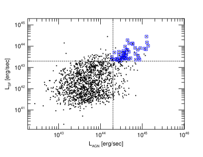
The next step was the selection of the most luminous LINERs within the chosen redshift interval. We measured first their AGN luminosity (LAGN) using the [OIII] $\lambda$ 5007 and [OI] $\lambda$ 6300 method of netzer09 (see Section LABEL:sec_agn_lum). The lines were initially corrected for reddening using the observed H $\alpha$ /H $\beta$ ratio and assuming galactic extinction (see Sections LABEL:sec_emission_measure and LABEL:sec_agn_lum). We selected a certain, statistically sufficient, fraction of 147 luminous LINERs with logLAGN $>$ 44.3 ergs/sec. We call these sources ’LLINERs’. Out of these sources we selected a luminosity limited sample of 47 galaxies with SF luminosity LSF $>$ 43.3 ergs/sec, where LSF is based on the Dn4000 index (see Section LABEL:sec_sfr). Of those, we were able to obtain the optical spectra for 42 LINERs and Herschel/PACS data for 6 sources. We refer to these 42 most luminous LINERs in terms of both AGN and SF luminosity as ’MLLINERs’. All observed MLLINERs are listed in Table 1, where we provide the basic information about their properties.
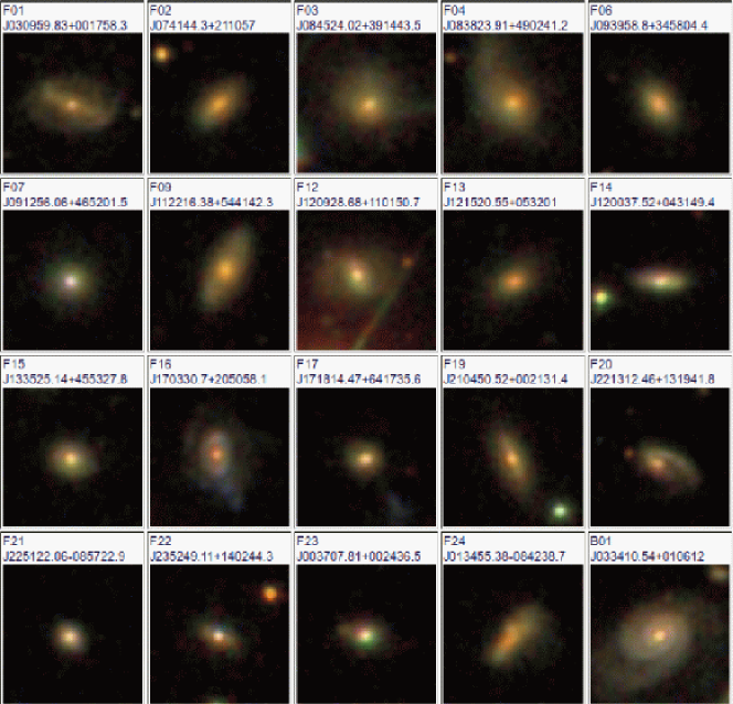
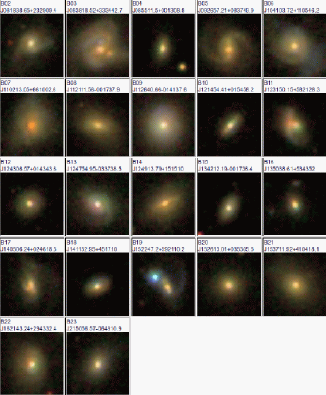
Figure 1 shows the position in the LAGN vs. LSF plane of the initially classified LINERs in the selected redshift range (black dots), and the final selected sample of MLLINERs (blue squares). Using the SDSS spectroscopy we estimated the AB continuum magnitude at 6500 Å (m6500). We used these magnitudes to divide the sample into ’faint’ and ’bright’ galaxies (m6500 $>$ 17.2 mag and m6500 $<$ 17.2 mag, respectively). These groups are marked with F or B in Table 1. We use this classification only for observational purposes. Figs 2 and 2 (Cont.) show SDSS colour images of all MLLINERs.

Refer to caption — Figure 1: The entire 0.04 $<$ z $<$ 0.11 SDSS/DR4 LINER sample used in this work (small black squares) and the sub-sample used for the Herschel proposal and the follow up spectroscopy (large blue squares). The dashed lines mark the lower limits on LAGN and LSF (based on Dn4000 index) used for the selection of the targets.

Table 1: Summary of observations.

ID	RA	DEC	z	m6500	morph	Date	seeing	pos. ang.	texp_b	texp_r	Area ${}_{nuc}$	IR data
	[deg]	[deg]		AB [mag]			[arc-sec]	[deg]	[sec]	[sec]	[arc-sec ${}^{2}$ ]
F01	47.499332	0.29955	0.098	18.53	S	02/11/2013	1.2	PA	3 $\times$ 3000.0	3 $\times$ 3000.0	3.6
F02	115.434586	21.18252	0.098	17.96	E	06/03/2014	1.2	314	3 $\times$ 3000.0	3 $\times$ 3000.0	3.6	1, 2
F03	131.35008	39.245438	0.109	17.63	P	08/03/2014	1.3	201	3 $\times$ 2000.0	3 $\times$ 2000.0	3.9
F04	129.59967	49.04478	0.101	17.58	P	08/03/2014	1.3	206	3 $\times$ 2400.0	3 $\times$ 2400.0	3.9
F06	144.995	34.96791	0.104	17.63	E	09/03/2014	1.4	220	3 $\times$ 2000.0	3 $\times$ 2000.0	4.2	2
F07	138.23363	46.8671	0.051	17.27	E	09/03/2014	1.4	338	3 $\times$ 1800.0	3 $\times$ 1800.0	4.2
F09	170.5683	54.6951	0.105	17.50	S	03/05/2014	1.4	149	3 $\times$ 2000.0	3 $\times$ 2000.0	4.2	2
F12	182.36954	11.030761	0.107	17.21	S	02/05/2014	1.6	410	3 $\times$ 2400.0	3 $\times$ 2400.0	6.0	2
F13	183.83566	5.533633	0.082	18.09	E	05/05/2014	1.2	120	3 $\times$ 3000.0	3 $\times$ 3000.0	3.6
F14	180.15637	4.530397	0.094	17.54	S	04/05/2014	1.2	265	3 $\times$ 2000.0	3 $\times$ 2000.0	3.6	2
F15	203.8548	45.891083	0.092	17.42	E	03/05/2014	1.4	239	3 $\times$ 1800.0	3 $\times$ 1800.0	4.2
F16	255.87796	20.849482	0.08	18.43	?	26/07/2014	1.0	184	3 $\times$ 3600.0	3 $\times$ 3600.0	3.0	2
F17	259.5603	64.29323	0.104	17.78	E	06/03/2014	1.2	213	3 $\times$ 2400.0	3 $\times$ 2400.0	3.6	1, 2
F19	316.2105	0.358728	0.091	17.90	?	25/07/2014	1.0	205	3 $\times$ 2800.0	3 $\times$ 2800.0	3.0	1
F20	333.30197	13.3283	0.103	18.53	P	27/07/2014	1.3	127	3 $\times$ 3600.0	3 $\times$ 3600.0	3.9
F21	342.84195	-8.956378	0.08	17.50	E	28/07/2014	1.6	241	3 $\times$ 3000.0	3 $\times$ 3000.0	4.8
F22	358.20468	14.04565	0.096	18.02	?	29/07/2014	1.2	238	3 $\times$ 3200.0	3 $\times$ 3200.0	3.6
F23	9.282583	0.410139	0.081	17.42	?	30/07/2014	1.4	260	3 $\times$ 2800.0	3 $\times$ 2800.0	4.2
F24	23.73075	-8.710756	0.092	18.02	P	09/10/2013	1.2	PA	3 $\times$ 3000.0	3 $\times$ 3000.0	3.6	2
B01	53.543957	1.103353	0.048	17.17	S	31/10/2013	1.5	PA	3 $\times$ 1600.0	3 $\times$ 1600.0	5.6
B02	124.66104	23.48597	0.103	16.90	P	07/03/2014	1.2	315	3 $\times$ 1700.0	3 $\times$ 1700.0	3.6	1
B03	129.57721	33.57853	0.062	16.79	P	06/03/2014	1.2	274	3 $\times$ 1600.0	3 $\times$ 1600.0	3.6	1, 2
B04	133.79796	0.219117	0.101	16.90	E	10/03/2014	1.3	255	3 $\times$ 1700.0	3 $\times$ 1700.0	3.9
B05	141.73837	8.630544	0.106	17.09	S	10/03/2014	1.3	180	3 $\times$ 1800.0	3 $\times$ 1800.0	3.9	2
B06*	160.26555	11.096189	0.053	16.50	?	01/05/2013	0.9	PA	4 $\times$ 900.0	3 $\times$ 900.0	3.0
B07	165.55441	66.1674	0.078	17.17	P	06/03/2014	1.2	245	3 $\times$ 1800.0	3 $\times$ 1800.0	3.6	1
B08*	170.29817	-0.293878	0.098	17.11	E	03/05/2013	0.9	PA	4 $\times$ 1200.0	4 $\times$ 900.0	3.0
B09	171.66946	-1.6938	0.046	15.93	E	10/03/2014	1.3	290	3 $\times$ 1200.0	3 $\times$ 1200.0	3.9
B10	183.72675	1.916183	0.099	16.98	?	10/03/2014	1.3	315	3 $\times$ 1700.0	3 $\times$ 1700.0	3.9
B11	187.959	58.35786	0.103	17.03	P	03/05/2014	1.4	446	3 $\times$ 1800.0	3 $\times$ 1800.0	4.2	2
B12	190.78575	1.728797	0.092	17.09	E	05/05/2014	1.2	238	3 $\times$ 1800.0	3 $\times$ 1800.0	3.6
B13*	191.979	-3.627378	0.09	16.59	S	03/05/2013	0.7	PA	2 $\times$ 1200.0	4 $\times$ 900.0	2.3	2
B14*	192.3075	15.252789	0.083	16.90	S	01/05/2013	0.7	PA	4 $\times$ 900.0	3 $\times$ 900.0	2.3
B15*	205.55083	-0.293453	0.086	17.17	E	02/05/2013	0.7	PA	3 $\times$ 900.0	4 $\times$ 900.0	2.3
B16	207.66092	53.73111	0.108	16.95	E	09/03/2014	1.4	267	3 $\times$ 1700.0	3 $\times$ 1700.0	4.2
B17	211.27605	2.771761	0.077	17.17	P	04/05/2014	1.2	180	3 $\times$ 1800.0	3 $\times$ 1800.0	3.6	2
B18	212.88733	45.28614	0.071	17.14	E	02/05/2014	1.6	109	3 $\times$ 1800.0	3 $\times$ 1800.0	6.0
B19*	230.6967	59.35285	0.076	17.09	P	01/05/2013	0.8	PA	4 $\times$ 1200.0	4 $\times$ 900.0	2.6
B20!*	231.55424	3.884864	0.086	16.79	E	02/05/2013	0.9	PA	3 $\times$ 1200.0	3 $\times$ 900.0	3.0
B21	234.29971	41.0717	0.098	16.68	E	28/07/2014	1.6	136	3 $\times$ 1800.0	3 $\times$ 1800.0	6.0
B22!	245.43016	29.725689	0.098	16.50	E	29/07/2014	1.2	264	3 $\times$ 1800.0	3 $\times$ 1800.0	3.6
B23	327.73575	-6.819708	0.059	16.68	E	26/07/2014	1.0	151	3 $\times$ 1800.0	3 $\times$ 1800.0	3.0

Column description: ID - MLLINER identification (sources observed with NOT are marked with ’*’; sources marked with ’!’ are possibly Sy2 galaxies and not LINERs as explained in Section LABEL:sec_emission_measure); RA, DEC - J2000 right ascension and declination in degrees; z - redshift, from SDSS public catalogues; m6500 - AB continuum magnitude at 6500 Å; morph - visual morphological classification where E, S, and P stand for Elliptical/S0, spiral, and peculiar (see the text); Date - date of observation; seeing - average FWHM of the seeing in arc-sec; pos. ang. - slit position angle in degrees (PA means that the paralactic angle was used, otherwise the angle is orientated along the major axis); texp_b and texp_r - total exposure time in blue and red parts in seconds; Area ${}_{nuc}$ - area covered with our ’nuclear’ extraction, in arc-sec ${}^{2}$ (just for comparison, the SDSS spectra cover an area of 7.08 arc-sec ${}^{2}$ ); IR data - availability of Herschel (1) and IRAS (2) data.

3 The Data

In this section we describe the optical spectroscopic observations and data reduction that we carried out for the 42 MLLINERs. We also describe the Herschel and IRAS FIR observations used in this project. To deal with catalogues we made use of TOPCAT (taylor05), while for spectral and displaying purposes we used SIPL code (Perea J.²²2http://www.iaa.es/ $\sim$ jaime/, priv. communication).

3.1 Optical spectroscopy

The observations were carried out during six runs (PI I. Márquez), between October 2013 and July 2014, using the Cassegrain Twin Spectrograph (TWIN) attached to the 3.5 m telescope at Calar Alto Observatory (CAHA³³3http://www.caha.es/, Almería, Spain). Table 1 summarises the information related with observations, including the date of observation, average seeing, position angle, and exposure times. As mentioned in the previous section, we observed 42 LINERs in total. We used the T01 (red) grating during all runs, covering a spectral range of 6700 Å - 8300 Å. In the blue, we used the T08 (3500 Å - 6500 Å) grism during the first two runs (October and November 2013), and T13 (3700 Å - 7000 Å) in the following ones. The spectral sampling for T01, T08, and T13 is 0.8, 1.1, and 2.1 Å/pix, respectively. The size of the slit used is 1.2 arc-sec for seeing $<$ 1.5 arc-sec, and 1.5 arc-sec for seeing $\geq$ 1.5 arc-sec. The values of seeing are listed in Table 1.
Additionally, ten bright MLLINERs were observed during four nights in May 2013 (PI I. Márquez) with the Andalucía Faint Object Spectrograph and Camera (ALFOSC) of the 2.5 m telescope at the Nordic Optical Telescope (NOT⁴⁴4http://www.not.iac.es/, Roque de los Muchachos Observatory, La Palma, Canary Islands, Spain). For six sources the S/N ratio was higher than for CAHA observations, and were consequently used throughout this work (marked with * in Table 1). We used #6 and #8 gratings, covering the spectral ranges 3200 Å - 5550 Å and 5825 Å - 8350 Å, in the blue and red, with a typical spectral sampling of 1.4 and 1.3 Å/pixel, respectively. We used a slit of 1.3 arc-sec in all observations. Several target exposures were taken (see Table 1) for cosmic rays and bad pixel removal. Arc lamp exposures were obtained before and after each target observation. At least two standard stars (up to four) were observed at the beginning and at the end of each night through a 10 arcsec width slit. For the final flux calibration we only considered the combination of those stars where the difference of their computed instrumental sensitivity function was lower than 10%.

Spectroscopic data reduction was carried out using IRAF⁵⁵5http://iraf.noao.edu. We followed the standard steps of bias subtraction, flat-field correction, wavelength calibration, atmospheric extinction correction, and flux calibration. The sky background level was determined by taking median averages over two strips on both sides of the galaxy signal, and subtracting it from the final combined galaxy spectra. As a sanity check, we compared the reduced and calibrated spectra with the SDSS ones, scaling our data to map similar areas. Good agreement was found between the two data sets, with differences lower than 20% in both, blue and red parts of the spectra.

Morphological classification was done visually, by three independent classifiers, using the SDSS $gri$ colour images shown in Figs 2 and 2 (Cont.). We separated all galaxies between early-type (E: ellipticals and lenticulars), spiral (S), and peculiar (P). The type represented in Table 1 is the one assigned by the majority of the classifiers (three or two). When the classification results in three different types, we leave the source unclassified (symbol ’?’ in the table). P class was assigned to those sources showing a clear presence of interactions, additional structures (e.g., tails, rings), and/or irregular shapes. More discussion about galaxy morphology is given in Section LABEL:sec_discussion_general_properties.

3.2 Far-infrared photometry

3.2.1 Herschel/PACS

We obtained FIR data for 6 objects in our sample (symbol 1 in column 13, Table 1) using the Photo detector Array Camera and Spectrometer (PACS) on board of the Herschel Space Observatory⁶⁶6http://www.esa.int/herschel. The data are part of a large LINER proposal (PI H. Netzer) out of which 6 targets were observed. We obtained 3 $\sigma$ photometry with PACS blue and red bands, at 70 and 160 $\mu$ m, respectively. The data were processed using the standard procedure and Herschel Interactive Processing Environment (HIPE) tool (ott06). We extracted flux densities and their errors using again the standard HIPE tools. The fluxes and their errors are listed in Table 2.

3.2.2 IRAS

We collected the available FIR flux measurements made by the Infrared Astronomical Satellite (IRAS⁷⁷7http://irsa.ipac.caltech.edu/IRASdocs/toc.html). Using the catalogue of galaxies and QSOs, Point Source Catalog (PSC), and Faint Source Catalog (FSC), we found 13 sources in total with flux densities measured or estimated as upper limits in all four IRAS bands, at 12, 25, 60 and 100 $\mu$ m. All these sources are listed in the last column of table 1, while the flux densities are provided in table 2. In the 60 $\mu$ m band, all detections have quality flag = 3 (high quality), while for the 100 $\mu$ m band, 10 detections have flag = 2 (moderate), and 3 sources have flag = 1 (upper limit). We only used the data with flags = 3 or = 2. For sources with flag = 1, we only used the information from the 60 $\mu$ m band (see Section LABEL:sec_sfr for more information).
Three of the IRAS observed sources (F02, F17, and B03) were also observed with Herschel/PACS. We compared the fluxes between PACS 70 $\mu$ m and IRAS 60 $\mu$ m, as well as the total SFRs measured with both surveys, and found only small differences. In the following analysis we will use the Herschel/PACS measurements for these three sources.

Table 2: Summary of FIR observations with Herschel and IRAS.

ID	Herschel_70	Herschel_160	IRAS_60	IRAS_100
F02	0.2911 $\pm$ 0.001	0.3909 $\pm$ 0.0024	0.2369 (3)	1.811 (1)
F06			0.2366 (3)	0.9363 (1)
F09			0.3957 (3)	0.9608 (2)
F12			0.4728 (3)	0.9564 (2)
F14			0.3074 (3)	0.6414 (2)
F16			0.5082 (3)	0.9774 (2)
F17	0.2894 $\pm$ 0.0036	0.2431 $\pm$ 0.0068	0.2993 (3)	0.4687 (1)
F19	0.02 $\pm$ 0.0011	0.0604 $\pm$ 0.0025
F24			0.2772 (3)	0.6128 (2)
B02	0.1153 $\pm$ 0.0037	0.1859 $\pm$ 0.0069
B03	0.7758 $\pm$ 0.0037	1.2186 $\pm$ 0.007	0.784 (3)	1.356 (2)
B05			0.2821 (3)	0.8639 (2)
B07	0.1229 $\pm$ 0.0037	0.3408 $\pm$ 0.0069
B11			0.289 (3)	0.6007 (2)
B13			0.7087 (3)	0.8789 (2)
B17			0.5019 (3)	0.9337 (2)

Column description: ID - MLLINER identification; Herschel_70 and Herschel_160 - FIR flux and its error in the 70 $\mu$ m and 160 $\mu$ m Herschel/PACS bands, respectively, in Jy; IRAS_60 and IRAS_100 - IRAS FIR flux and the quality flag in 60 $\mu$ m and 100 $\mu$ m bans, respectively, in Jy (quality flag is given between the brackets, where 3 means high quality, 2 moderate quality, and 1 an upper limit).

4 Data Analysis and Measurements

4.1 Dn4000 and H $\delta$ measurements

Using the flux calibrated spectra, we measured the strength of 4000 $\AA$ break (Dn4000) and Balmer absorption-line index H $\delta$ . These two indices are known to be important for tracing the star formation histories (SFH) in galaxies (kauffmann03). Dn4000 was measured as explained in balogh99, as the ratio between the average flux density in the continuum bands 4000 - 4100 $\AA$ and 3850 - 3950 $\AA$ . To obtain the H $\delta$ index we used the definition of worthey97. We first measured the average fluxes in two continuum bandpasses, blue (4041.60 - 4079.75 $\AA$ ), and red (4128.50 - 4161.00 $\AA$ ). The two average fluxes defined the continuum which we used to measure the H $\delta$ index, carrying out the integration within the feature in the band 4083.50 - 4122.25 $\AA$ and expressing it in terms of the equivalent width. Table 3 lists all these values. The main purpose of measuring Dn4000 is for using it later as a SFR indicator, while H $\delta$ was mainly used as an additional parameter of consistency of our measurements when comparing it with Dn4000. Previous works showed that the typical values for early-type galaxies are Dn4000 $>$ 1.7 and H $\delta$ $<$ 1 (kauffmann03a).
We compared our Dn4000 and H $\delta$ measurements with those from the MPA-JHU DR7 database measured on SDSS spectra (brinchmann04). In general, for both parameters we found a good agreement between the two, with Spearman’s rank correlation coefficients p = 0.81 and 0.84, when comparing Dn4000 and H $\delta$ , respectively.

Table 3: Dn4000 and H

\delta

measurements.

ID	Dn4000	H $\delta$	ID	Dn4000	H $\delta$
F01	1.32 $\pm$ 0.37	0.90	B03		3.16
F02	1.37 $\pm$ 0.28	3.70	B04	1.47 $\pm$ 0.31	4.67
F03	1.45 $\pm$ 0.34	2.81	B05	1.41 $\pm$ 0.32	3.54
F04	1.51 $\pm$ 0.34	0.85	B06	1.30 $\pm$ 0.22	5.59
F06	1.35 $\pm$ 0.27	5.20	B07	1.39 $\pm$ 0.34	1.26
F07		7.46	B08	1.43 $\pm$ 0.24	2.07
F09	1.44 $\pm$ 0.35	2.97	B09
F12	1.49 $\pm$ 0.40	5.44	B10	1.28 $\pm$ 0.23	4.10
F13		5.59	B11	1.26 $\pm$ 0.15	3.54
F14	1.37 $\pm$ 0.30	4.16	B12	1.33 $\pm$ 0.28	0.83
F15	1.33 $\pm$ 0.27	4.93	B13	1.01 $\pm$ 0.12	4.52
F16	1.16 $\pm$ 0.25	0.66	B14	1.52 $\pm$ 0.26	1.28
F17	1.26 $\pm$ 0.29	7.80	B15	1.27 $\pm$ 0.25	7.04
F19	1.39 $\pm$ 0.33	0.24	B16	1.36 $\pm$ 0.30	6.23
F20	1.16 $\pm$ 0.20	2.25	B17	1.21 $\pm$ 0.27	6.90
F21	1.37 $\pm$ 0.30	5.98	B18	1.34 $\pm$ 0.26	6.00
F22	1.17 $\pm$ 0.18	4.94	B19	1.32 $\pm$ 0.27	7.21
F23	1.30 $\pm$ 0.27	6.48	B20!	1.42 $\pm$ 0.27	3.20
F24	1.32 $\pm$ 0.56	8.26	B21	1.45 $\pm$ 0.27	0.24
B01	1.23 $\pm$ 0.29	5.49	B22!	1.22 $\pm$ 0.23	5.79
B02	1.16 $\pm$ 0.22	6.35	B23	1.46 $\pm$ 0.27	5.96

! possibly Sy2 galaxies (see Section LABEL:sec_emission_measure)

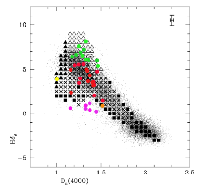
Figure 3 shows the relation between the Dn4000 and H $\delta$ indices obtained by kauffmann03 for the SDSS DR4 sample (see their figure 6). They used a library of 32,000 different SFH, where for each SFH they have a corresponding Dn4000 and H $\delta$ indices, as well as the fraction of the total stellar mass of the galaxy formed in the bursts over the past 2 Gyr (F ${}_{burst}$ ). In their figure the bins are coded according to the fraction of model SFHs with F ${}_{burst}$ in a given range (see the caption of their Fig. 3). We used this figure and overplotted our Dn4000 and H $\delta$ measurements (coloured filled circles). In general our measurements are consistent with the models by kauffmann03. More details about star formation histories are given in Section LABEL:sec_discussion_general_properties.

4.2 STARLIGHT spectral fittings of the nuclear regions

We extracted what we call the nuclear spectra by selecting a central region equal to 2.5 times the FWHM of the seeing. In the case of CAHA the extraction size is 5 -8 pixels (depending on the used slit), while in the case of NOT data the central 10 pixels were extracted. The total area covered by the nuclear extraction is given in the last column of Table 1 for all MLLINERs.
Modelling of the nuclear stellar spectra of our sources was performed with the STARLIGHT⁸⁸8http://astro.ufsc.br/starlight V.04 synthesis code (cid05; cid09). All spectra were previously corrected for galactic extinction, K-corrected, and moved to rest-frame. To correct for the galactic extinction we used the pystarlight⁹⁹9https://pypi.python.org/pypi/PySTARLIGHT library within the astrophysics Python package¹⁰¹⁰10https://pythonhosted.org/Astropysics/ and schlegel98 maps of dust IR emission. Our fittings are based on the templates from bruzual03, with solar metallicity and 25 different stellar ages, from 0.001 $\times$ 10 ${}^{9}$ to 18 $\times$ 10 ${}^{9}$ . Considering that we are dealing with nuclear spectra of large galaxies, this approximation should be fine for our sources (ho03; ho08). We masked in all spectra the emission line regions, areas with atmospheric absorptions, and regions with bad pixels. To measure the signal-to-noise (S/N) we checked visually all spectra to select the continuum region free of bad pixels, using always the blue range and a width of at least 80Å. In most cases we selected the region around $\sim$ 4600Å or $\sim$ 5600Å. S/N measurements are listed in Table 4.
In this work we used the cardelli89 extinction law. This law was widely used in different surveys for fitting the host-dominated sources (stasinska06; cid11; gonzalezdelgado16). We also tested the calzetti07 law, and made a comparison between the two. We found differences to be lower than 20% therefore we only show results that were obtained with the Cardelli et al (1989) extinction law.

The basic information obtained from the best fit stellar population models is summarised in Table 4 for all MLLINERs. The adev parameter gives the goodness of the fit, and presents the mean deviation over the all fitted pixels (in percentage); adev $<$ 6 and $<$ 10 stand for ’very good’ and ’good’ fits, respectively (cid05; cid09). We obtained very good fit in $\sim$ 80% of the cases. The measured S/N ratio and extinction A ${}_{V}$ are given in columns 3 and 4, respectively. The best fit parameters (M_cor_tot and M_ini_tot) were used to measure two types of stellar masses, following cid05; cid09:
the present mass in stars,

M ${}_{*}$ = M_cor_tot $\times$ 10 ${}^{-17}\,$ $\times$ 4 $\pi$ d ${}^{2}$ $\times$ (3.826 $\times$ 10 ${}^{33}$ ) ${}^{-1}$ ,

and the initial mass, that has been processed into stars throughout the galaxy life:

M ${}_{*}^{ini}$ = M_ini_tot $\times$ 10 ${}^{-17}\,$ $\times$ 4 $\pi$ d ${}^{2}$ $\times$ (3.826 $\times$ 10 ${}^{33}$ ) ${}^{-1}$ .

The results regarding the best stellar population mixture are summarised in columns 7 - 9. They are represented through the light-fraction population vector (corresponds to the same wavelength selected for measuring S/N, see above) for three stellar ages: young (with age [yr] $\leq$ 10 ${}^{8}$ ), intermediate (10 ${}^{8}$ $<$ age [yr] $\leq$ 10 ${}^{9}$ ), and old (age [yr] $>$ 10 ${}^{9}$ ). We discuss stellar populations in more detail in Section LABEL:sec_discussion_general_properties. Finally, we calculated the light-weighted mean ages of our MLLINERs, using as a reference cid13:

$<$ logt $>$ = $\sum\limits_{t,Z}$ $x_{t,Z}$ logt,

where $x_{t,Z}$ is a fraction of light at stellar age t in our best-fit model and metallicity Z (Z ${}_{\odot}$ in our case). The example with the best-fit models (red lines) and original spectra (blue lines) are shown in Appendix A (Figs. LABEL:fig_spectra_1).

Table 4: The best stellar population mixture found by STARLIGHT.

ID	adev	S/N	A ${}_{V}$	M ${}_{*}$	M ${}_{*}^{ini}$	stpop1	stpop2	stpop3	$<$ logt $>$	ID	adev	S/N	A ${}_{V}$	M ${}_{*}$	M ${}_{*}^{ini}$	stpop1	stpop2	stpop3	$<$ logt $>$
F01	9.62	15.16	0.138	0.76	1.46	4.83	22.08	71.42	9.03	B03	2.64	44.51	0.877	2.89	5.79	15.81	14.67	67.75	9.19
F02	4.70	21.69	1.667	2.50	4.70	15.17	18.92	66.47	8.97	B04	3.54	44.18	0.584	1.93	3.41	0.0	0.0	93.51	8.61
F03	4.59	25.82	0.584	1.67	3.12	6.38	0.0	95.8	9.53	B05	4.39	30.96	0.753	3.77	7.20	1.72	3.4	88.68	8.77
F04	4.27	26.74	0.827	2.17	4.07	6.89	0.0	97.81	9.82	B06	2.68	45.25	1.209	3.35	6.65	0.0	55.28	42.89	8.95
F06	3.74	36.17	1.306	1.56	2.64	5.64	10.51	79.16	8.51	B07	4.26	37.31	2.209	6.81	13.63	8.55	20.57	70.08	9.46
F07	3.37	27.42	1.162	0.61	1.21	41.52	42.3	18.26	8.17	B08	3.43	31.36	0.388	4.64	9.29	0.0	53.01	49.76	9.45
F09	8.49	18.36	1.423	1.93	3.44	0.0	10.96	90.84	9.36	B09	2.60	44.41	0.234	0.96	1.77	9.18	0.0	87.64	8.97
F12	5.21	31.79	0.459	0.86	1.56	0.0	43.09	54.45	9.06	B10	3.23	47.73	0.787	1.19	2.02	5.21	12.4	78.21	8.59
F13	12.60	23.90	1.515	0.58	0.99	0.0	4.24	90.83	8.71	B11	3.43	43.65	0.517	1.68	2.95	0.0	14.94	75.46	8.26
F14	7.53	20.31	0.8	1.10	2.04	0.0	89.94	8.7	8.94	B12	5.66	27.73	0.706	0.57	0.97	0.0	24.78	70.88	8.7
F15	5.09	28.67	0.991	1.05	1.87	0.0	96.77	3.39	8.99	B13	2.17	50.33	0.673	1.44	2.47	7.65	65.0	26.36	8.18
F16	7.51	17.07	1.239	0.88	1.70	16.44	12.77	69.52	8.69	B14	3.39	41.95	0.741	4.75	9.42	0.0	25.8	74.38	9.5
F17	3.55	43.21	1.369	1.02	1.71	7.1	32.41	58.34	8.58	B15	2.89	43.62	0.701	1.03	1.85	0.0	92.53	9.72	9.0
F19	7.39	18.17	0.542	1.54	2.98	0.0	17.79	83.21	9.68	B16	3.49	39.68	0.327	1.33	2.31	0.0	0.0	98.71	9.07
F20	6.51	22.11	1.154	0.90	1.69	6.37	47.45	46.19	8.68	B17	3.95	45.53	0.997	1.47	2.83	0.0	57.78	42.84	9.07
F21	7.49	22.74	0.738	1.52	2.84	0.0	49.74	50.4	9.27	B18	4.38	32.81	0.916	1.44	2.78	0.0	78.52	18.81	8.88
F22	4.30	30.01	0.698	1.45	2.81	0.0	49.72	48.15	8.75	B19	4.48	33.10	1.914	5.61	11.06	0.0	77.21	21.86	8.76
F23	5.25	34.38	0.702	1.12	2.13	0.0	86.75	9.27	8.58	B20!	3.20	31.32	0.312	5.41	10.82	0.0	51.55	53.01	9.9
F24	11.55	10.97	1.68	1.78	3.52	12.06	57.86	31.98	8.98	B21	4.41	51.15	0.515	8.32	16.65	0.0	38.45	56.92	9.28
B01	5.67	23.82	0.681	0.69	1.36	2.67	74.6	23.11	8.72	B22!	3.71	42.86	0.462	4.85	9.52	0.0	57.46	36.84	8.69
B02	2.87	41.10	1.105	3.89	7.65	9.67	55.18	32.08	8.45	B23	4.26	35.50		1.73	3.31	0.0	63.79	34.14	9.11

Column description: ID - MLLINER identification (’!’ - possibly Sy2 galaxies, see Section LABEL:sec_emission_measure); adev - goodness of the fit (see the text); S/N - measured signal-to-noise ratio (see Section 4.2); A ${}_{V}$ - extinction in V band; M ${}_{*}$ and M ${}_{*}^{ini}$ - current and initial mass in stars, respectively, in 10 ${}^{10}$ [M ${}_{\odot}$ ]; stpop1 - fraction of young stars with age [yr] $\leq$ 10 ${}^{8}$ in %; stpop2 - fraction of intermediate stars with 10 ${}^{8}$ $<$ age [yr] $\leq$ 10 ${}^{9}$ in %; stpop3 - fraction of old stars with age [yr] $>$ 10 ${}^{9}$ in %; $<$ logt $>$ - mean age.